Acknowledgments

Probably these first pages of a PhD thesis are the most widely read pages from entire publication. In that place you can find people who means something in my 5 year life of PhD candidate.

First and foremost, I would like to acknowledge my thesis advisor, Assoc. Prof. Mai Suan Li, for his superb mentorship. His broad knowledge, experience, patience and encouragement helped guide me throughout the duration of this work. The dedication of his time and energy was one of the main reasons that I was able to finish this challenging work. He is a excellent advisor who has taught me a lot about things in science to succeed in research. I really enjoyed the time spent with him.

I would like to thank prof. Chin-Kun Hu for providing me with sufficient funds and an opportunity to work in his lab to conduct my research during my visits in Taiwan.

I also would like to thank P. Bialokozewicz and P. Janiszewski for the useful discussions and the valuable remarks and tips about linux software.

I am very grateful to the Polish Committee for UNESCO for the financial support.

Lastly, I would like to attribute my largest credit to my family in Poland, Belarus and Russia. Their love and dedication always gave me an enormous amount of power to overcome all the obstacles when I got exhausted.

Chapter 1 Introduction

Proteins are biomolecules that perform and control almost all functions in all living organisms. Their biological functions include catalysis (enzymes), muscle contraction (titin), transport of ions (hemoglobin), transmission of information between specific cells and organs (hormones), activities in the immune system (antibodies), passage of molecules across cell membranes etc. The long process of life evolution has designed proteins in the natural world in such a mysterious way that under normal physiological conditions (pH $\approx$ 7, $T$ = 20-40 C, atmospheric pressure) they acquire well defined compact three-dimensional shapes, known as the native conformations. Only in these conformation proteins are biologically active. Proteins unfold to more extended conformations, if the mentioned above conditions are changed or upon application of denaturant agents like urea or guanidinum chloride. If the physiological conditions are restored, then most of proteins refold spontaneously to their native states Anfinsen_Science73 . Proteins can also change their shape, if they are subjected to an external mechanical force.

The protein folding theory deals with two main problems. One of them is a prediction of native conformation for a given sequence of amino acids. This is referred to as the protein folding. The another one is a design problem (inverse folding), where a target conformation is known and one has to find what sequence would fold into this conformation. The understanding of folding mechanisms and protein design have attracted an intensive experimental and theoretical interest over the past few decades as they can provide insights into our knowledge about living bodies. The ability to predict the folded form from its sequence would widen the knowledge of genes. The genetic code is a sequence of nucleotides in DNA that determines amino acid sequences for protein synthesis. Only after synthesis and completion of folding process proteins can perform their myriad functions.

In the protein folding problem one achieved two major results. From the kinetics prospect, it is widely accepted that folding follows the funnel picture, i.e. there exist a numerous number of routes to the native state (NS) Leopold_PNAS92 . The corresponding free energy landscape (FEL) looks like a funnel. This new point of view is in sharp contrast with the picture Baldwin_Nature94 , which assumes that the folding progresses along a single pathway. The funnel theory resolved the so called Lenvithal paradox Levinthal_JCP68 , according to which folding times would be astronomically large, while proteins in vivo fold within $\mu$s to a few minutes. From the thermodynamics point of view, both experiment and theory showed that the folding is highly cooperative Ptitsyn_book . The transition from a denaturated state (DS) to the folded one is first order. However, due to small free energies of stability of the NS, relative to the unfolded states ($5-20k_{B}T$), the possibility of a marginally second order transition is not excluded MSLi_PRL04 .

Recently Fernandez and coworkers Fernandez_Sci04 have carried out force clamp experiments in which proteins are forced to refold under the weak quenched force. Since the force increases the folding time and initial conformations can be controlled by the end-to-end distance, this technique facilitates the study of protein folding mechanisms. Moreover, by varying the external force one can estimate the distance between the DS and transition state (TS) Fernandez_Sci04 ; MSLi_PNAS06 or, in other words, the force clamp can serve as a complementary tool for studying the FEL of biomolecules.

After the pioneering AFM experiment of Gaub et al. Florin_Science94 , the study of mechanical unfolding and stability of biomolecules becomes flourish. Proteins are pulled either by the constant force, or by force ramped with a constant loading rate. An explanation for this rapidly developing field is that single molecules force spectroscopy (SMFS) techniques have a number of advantages compared to conventional folding studies. First, unlike ensemble measurements, it is possible to observe differences in nature of individual unfolding events of a single molecule. Second, the end-to-end distance is a well-defined reaction coordinate and it makes comparison of theory with experiments easier. Remember that a choice of a good reaction coordinate for describing folding remains elusive. Third, the single molecule technique allows not only for establishing the mechanical resistance but also for deciphering FEL of biomolecules. Fourth, SMFS is able to reveal the nature of atomic interactions. It is worthy to note that studies of protein unfolding are not of academic interest only. They are very relevant as the unfolding plays a critically important role in several processes in cells Matoushek_COSP03 . For example, unfolding occurs in process of protein translocation across some membranes. There is reversible unfolding during action of proteins such a titin. Full or partial unfolding is a key step in amyloidosis.

Despite much progress in experiments and theory, many questions remain open. What is the molecular mechanism of protein folding of some important proteins? Can we use approximate theories for them? Does the size of proteins matter for the cooperativity of the folding-unfolding transition? One of the drawbacks of the force clamp technique Fernandez_Sci04 is that it fixes one end of a protein. While thermodynamic quantities do not depend on what end is anchored, folding pathways which are kinetic in nature may depend on it. Then it is unclear if this technique probes the same folding pathways as in the case when both termini are free. Although in single molecule experiments, one does not know what end of a biomolecule is attached to the surface, it would be interesting to know the effect of end fixation on unfolding pathways. Predictions from this kind of simulations will be useful at a later stage of development, when experimentalists can exactly control what end is pulled. Recently, experiments Brockwell_NSB03 ; Dietz_PNAS06a have shown that the pulling geometry has a pronounced effect on the unfolding free energy landscape. The question is can one describe this phenomenon theoretically. The role of non-native interactions in mechanical unfolding of proteins remains largely unknown. It is well known that an external force increases folding barriers making the configuration sampling difficult. A natural question arises is if one can can develop a efficient method to overcome this problem. Such a method would be highly useful for calculating thermodynamic quantities of a biomolecule subjected to an mechanical external force.

In this thesis we address the following questions.

1. We have studied the folding mechanism of the protein domain hbSBD (PDB ID: 1ZWV) of the mammalian mitochondrial branched-chain $\alpha$-ketoacid dehydrogenase (BCKD) complex in detail, using Langevin simulation and CD experiments. Our results support its two-state behavior.

2. The cooperativity of the denaturation transition of proteins was investigated with the help of lattice as well as off-lattice models. Our studies reveal that the sharpness of this transition enhances as the number of amino acids grows. The corresponding scaling behavior is governed by an universal critical exponent.

3. It was shown that refolding pathways of single $\alpha\beta$-protein ubiquitin (Ub) depend on what end is anchored to the surface. Namely, the fixation of the N-terminal changes refolding pathways but anchoring the C-terminal leaves them unchanged. Interestingly, the end fixation has no effect on multi-domain Ub.

4. The FEL of Ub and fourth domain of Dictyostelium discoideum filamin (DDFLN4) was deciphered. We have studied the effect of pulling direction on the FEL of Ub. In agreement with the experiments, pulling at Lys48 and C-terminal increases the distance between the NS and TS about two-fold compared to the case when the force is applied to two termini.

5. A new force replica exchange (RE) method was developed for efficient configuration sampling of biomolecules pulled by an external mechanical force. Contrary to the standard temperature RE, the exchange is carried out between different forces (replicas). Our method was successfully applied to study thermodynamics of a three-domain Ub.

6. Using the Go modeling and all-atom models with explicit water, we have studied the mechanical unfolding mechanism of DDFLN4 in detail. We predict that, contrary to the experiments of Rief group Schwaiger_NSB04 , an additional unfolding peak would occur at the end-to-end $\Delta R\approx 1.5$nm in the force-extension curve. Our study reveals the important role of non-native interactions which are responsible for a peak located at $\Delta R\approx 22$nm. This peak can not be encountered by the Go models in which the non-native interactions are neglected. Our finding may stimulate further experimental and theoretical studies on this protein.

My thesis is organized as follows:

Chapter 2 presents basic concepts about proteins. Experimental and theoretical tools for studying protein folding and unfolding are discussed in Chapter 3. Our theoretical results on the size dependence of the cooperativity index which characterizes the sharpness of the melting transition are provided in Chapter 4. Chapter 5 is devoted to the simulation of the hbSBD domain using the Go-modeling. Our new force RE and its application to a three-domain Ub are presented in Chapter 6. In Chapter 7 and 8 I presented results concerning refolding under quench force and unfolding of ubiquitin and its trimer. Both, mechanical and thermal unfolding pathways will be presented. The last Chapters 9 and 10 discuss the results of all-atom molecular dynamics and Go simulations for mechanical unfolding of the protein DDFLN4. The results presented in this thesis are based on the following works:

1. M. Kouza, C.-F. Chang, S. Hayryan, T.-H. Yu, M. S. Li, T.-H. Huang, and C.-K. Hu, Biophysical Journal 89, 3353 (2005).

2. M. Kouza, M. S. Li, E. P. O’Brien Jr., C.-K. Hu, and D. Thirumalai, Journal of Physical Chemistry A 110, 671 (2006)

3. M. S. Li, M. Kouza, and C.-K. Hu, Biophysical Journal 92, 547 (2007)

4. M. Kouza, C.-K. Hu and M. S. Li, Journal of Chemical Physics 128, 045103 (2008).

5. M. S. Li and M. Kouza, Dependence of protein mechanical unfolding pathways on pulling speeds, submitted for publication.

6. M. Kouza, and M. S. Li, Protein mechanical unfolding: importance of non-native interactions, submitted for publication.

Chapter 2 Basic concepts

2.1 What is protein?

The word ”protein” which comes from Greek means ”the primary importance”. As mentioned above, they play a crucial role in living organisms. Our muscles, organs, hormones, antibodies and enzymes are made up of proteins. They are about 50% of the dry weight of cells. Proteins are used as a mediator in the process of how the genetic information moves around the cell or in another words transmits from parents to children (Fig. 1). Composed of DNA, genes keep the genetic code as it is a basic unit of heredity. Our various characteristics such as color of hair, eyes and skin are determined after very complicated processes. In brief, at first linear strand of DNA in gene is transcribed to mRNA and this information is then ”translated” into a protein sequence. Afterwards proteins start to fold up to get biologically functional three-dimensional structures, such as various pigments, enzymes and hormones. One protein is responsible for skin color, another one - for hair color. Hemoglobin gives the color of our blood and carry out the transport functions, etc. Therefore, proteins perform a lot of diverse functions and understanding of mechanisms of their folding/unfolding is essential to know how a living body works.

Figure 1: The connection between genetic information, DNA and protein. This image and the rest of molecular graphics in this dissertation were made using VMD VMD , xmgrace, xfig and gimp software.

The number of proteins is huge. The protein data bank (http://www.rcsb.org) contains about 54500 protein entries (as of November 2008) and this number keeps growing rapidly. Proteins are complex compounds that are typically constructed from one set of 20 amino acids. Each amino acid has an amino end ( $-NH_{2}$) and an acid end (carboxylic group -COOH). In the middle of amino acid there is an alpha carbon to which hydrogen and one of 20 different side groups are attached (Fig. 2a). The structure of side group determines which of 20 amino acids we have. The simplest amino acid is Glysine, which has only a single hydrogen atom in its side group. Other aminoacids have more complicated construction, that can contain carbon, hydrogen, oxygen, nitrogen or sulfur (e.g., Fig. 2b).

Amino acids are denoted either by one letter or by three letters. Phenylalanine, for example, is labeled as Phe or F. There are several ways for classification of amino acids. Here we divide them into four groups basing on their interactions with water, their natural solvent. These groups are:

1. Alanine (Ala/A), Isoleucine (Ile/I), Leucine (Leu/L), Methionine (Met/M), Phenylalanine (Phe/F), Proline (Pro/P), Tryptophan (Trp/W), Valine (Val/V).

2. Asparagine (Asn/N), Cysteine (Cys/C), Glutamine (Gln/Q), Glycine (Gly/G), Serine (Ser/S), Threonine (Thr/T), Tyrosine (Tyr/Y).

3. Arginine (Arg/R), Histidine (His/H), Lysine (Lys/K).

4. Aspartic acid (Asp/D), Glutamic acid (Glu/E).

Figure 2: (a) Components of an amino acid: C - central carbon atom, H - hydrogen atom, $H_{3}N$ - amino group, $COO^{-}$ - carboxyl group, R - radical group. (b) Examples of three amino acids, which shows the differences in radical groups. (c) Formation of a peptide bond. The carboxyl group of amino acid 1 is linked to the adjacent amino group of amino acid 2.

Here one and three-letter notations of amino acids are given in brackets. Group 1 is made of non polar hydrophobic residues. The three other groups are made of hydrophilic residues. From an electrostatic point of view, groups 2, 3 and 4 contain polar neutral, positively charged and negatively charged residues, respectively.

In order to make proteins, amino acids link together in long chains by a chemical reaction in which a water molecule is released and thus peptide bond is created (Fig. 2c). Hence, protein is a chain of amino acids connected via peptide bonds having free amino group at one end and carboxylic group at the other one. The sequence of linked amino acids is known as a primary structure of a protein (Fig. 3a). The structure is stabilized by hydrogen bonding between the amine and carboxylic groups. Pauling and CoreyPauling_PNAS51a ; Pauling_PNAS51b theoretically predicted that proteins should exhibit some local ordering, now known as secondary structures. Based on energy considerations, they showed that there are certain regular structures which maximize the number of hydrogen bonds (HBs) between the C-O and the H-N groups of the backbone. Depending on angles between the carbon and the nitrogen, and the carbon and carboxylic group, the secondary structures may be either alpha-helices or beta-sheets (Fig. 3b). Helices are one-dimensional structures, where the HBs are aligned with its axis. There are 3.6 amino acids per helix turn, and the typical size of a helix is 5 turns. $\beta$-strands are quasi two-dimensional structures. The H-bonds are perpendicular to the strands. A typical $\beta$-sheet has a length of 8 amino acids, and consists of approximately 3 strands. In addition to helices and beta strands, secondary structures may be turns or loops. The third type of protein structure is called tertiary structure (Fig. 3c). It is an overall topology of the folded polypeptide chain. A variety of bonding interactions between the side chains of the amino acids determines this structure. Finally, the quaternary structure (Fig. 3d) involves multiple folded protein molecules as a multi-subunit complex.

Figure 3: Levels of protein structures. (a) An example of primary structures or sequences. (b) Alpha helix and beta strand are main secondary structures. The green dashed lines shows HBs. (c) Tertiary structure of protein (PDB ID: 2CGP). (d) Quaternary structure from two domains (PDB ID: 1CGP).

2.2 The possible states of proteins

Although it was long believed that proteins are either denaturated or native, it seems now well established that they may exist in at least three different phases. The following classification is widely accepted:

1. Native state
   In this state, the protein is said to be folded and has its full biological activity. Three dimensional native structure is well-defined and unique, having a compact and globular shape. Basically, the conformational entropy of the NS is zero.

2. Denaturated states
   These states of proteins lack their biological activity. Depending on external conditions, there exists at least two denaturated phases:

   1. Coil state
      In this state, a denaturated protein has no definite shape. Although there might be local aggregation phenomena, it is fairly well described as the swollen phase of a homopolymer in a good solvent. Coil state has large conformational entropy.

   2. Molten globule
      At low pH (acidic conditions), some proteins may exist in a compact state, named “molten globule” Ptitsyn_book . This state is compact having a globular shape, but it does not have a well defined structure and bears strong resemblance to the collapsed phase of a homopolymer in a bad solvent. It is slightly less compact than the NS, and has finite conformational entropy.

In vitro, the transition between the various phases is controlled by temperature, pH, denaturant agent such as urea or guanidinum chloride.

2.3 Protein folding

Protein folding is a process in which a protein reaches the NS starting from denaturated ones. Understanding this complicated process has attracted attention of researchers for over forty years. Although a number of issues remain unsolved, several universal features have been obtained. Here we briefly discuss the state of art of this field.

2.3.1 Experimental techniques

To determine protein structures one mainly uses the X-ray crystallography Kendrew_Nature60 and NMR Bax_JBNMR97 . About 85% of structures that have been deposited in Protein Data Bank was determined by X-ray diffraction method. NMR generally gives a worse resolution compared to X-ray crystallography and it is limited to relatively small biomolecules. However, this method has the advantage that it does not require crystallization and permits to study proteins in their natural environments.

Since proteins fold within a few microseconds to seconds, the folding process can be studied using the fluorescence, circular dichroism (CD) etc Nolting_book . CD, which is directly related to this thesis, is based on the differential absorption of left- and right-handed circularly polarized light. It allows for determination of secondary structures and also for changes in protein structure, providing possibility to observe folding/unfolding transition experimentally. As the fraction of the folded conformation $f_{N}$ depends on the ellipticity $\theta$ linearly (see Eq. 37 below), one can obtain it as a function of $T$ or chemical denaturant by measuring $\theta$.

2.3.2 Thermodynamics of folding

The protein folding is a spontaneous process which obeys the main thermodynamical principles. Considering a protein and solvent as a isolated system, in accord with the second thermodynamic law, their total entropy has the tendency to increase, $\Delta S_{prot}+\Delta S_{sol}\geq 0$. Here $\Delta S_{prot}$ and $\Delta S_{sol}$ are the protein and solvent entropy. If a protein absorpts from the environment heat $Q$, then $\Delta S_{prot}=-\frac{Q}{T}$ ($-Q$ is the heat obtained by the solvent from the protein). Therefore, we have $Q-T\Delta S_{prot}\leq 0$. In the isobaric process, $\Delta H=Q$ as the system does not perform work, where $H$ is the enthalpy. Assuming $\Delta G=\Delta H-T\Delta S_{prot}$, we obtain

$$\Delta G=\Delta H-T\Delta S_{prot}\leq 0.$$ (1)

In the isothermic process ($T$=const), $G$ in Eq. (1) is the Gibbs free energy of protein ($G=H-TS_{prot}$). Thus the folding proceeds in such a way that the Gibbs free energy decreases. This is reasonable because the system always tries to get a state with minimal free energy. As the system progresses to the NS, $\Delta S_{prot}$ should decrease disfavoring the condition (1). However, this condition can be fulfilled, provided $\Delta H$ decreases. One can show that this is the case taking into account the hydrophobic effect which increases the solvent entropy (or decrease of $H$) by burying hydrophobic residues in the core region Fersht_book . Thus, from the thermodynamics point of view the protein folding process is governed by the interplay of two conflicting factors: (a) the decrease of configurational entropy humps the folding and (b) the increase of the solvent entropy speeds it up.

2.3.3 Levinthal’s paradox and funnel picture of folding

Let us consider a protein which has only 100 amino acids. Using a trivial model where there are just two possible orientations per residue, we obtain $2^{100}$ possible conformational states. If one assumes that an jump from one conformation to the another one requires 100 picoseconds, then it would take about $5\times 10^{8}$ years to check up all the conformations before acquiring the NS. However, in reality, typical folding times range from microseconds to seconds. It is quite surprising that proteins are designed in such a way, that they can find correct NS in very short time. This puzzle is known as Levinthal’s paradoxLevinthal_JCP68 .

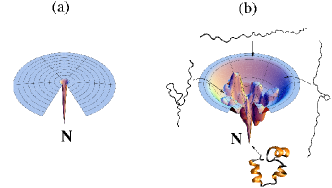
Figure 4: (a) Flat energy landscape, which corresponds to blind search for the NS. (b) Funnel-like FEL proposed by Wolynes and co-workers.

To resolve this paradox, Wolynes and coworkers Leopold_PNAS92 ; Onuchic_COSB04 propose the theory based on the folding FEL. According to their theory, the Levinthal’s scenario or the old view corresponds to random search for the NS on a flat FEL (Fig. 4a) traveling along a single deterministic pathway. Such a blind search would lead to astronomically large folding times. Instead of the old view, the new view states that the FEL has a ”funnel”-like shape (Fig. 4b) and folding pathways are multiple. If some pathways get stuck somewhere, then other pathways would lead to the NS. In the funnel one can observe a bottleneck region which corresponds to an ensemble of conformations of TS. By what ever pathway a protein folds, it has to overcome the TS (rate-limiting step). The folding on a rugged FEL is slower than on the smooth one due to kinetic traps.

It should be noted that very likely that the funnel FEL occurs only in systems which satisfy the principle of minimal frustration Bryngelson_PNAS87 . Presumably, Mother Nature selects only those sequences that fulfill this principle. Nowadays, the funnel theory was confirmed both theoretically Clementi_JMB00 ; Koga_JMB01 and experimentally Jin_Structure03 and it is widely accepted in the scientific community.

2.3.4 Folding mechanisms

The funnel theory gives a global picture about folding. In this section we are interested in pathways navigated by an ensemble of denaturated states of a polypeptide chain en route to the native conformation. The quest to answer this question has led to discovering diverse mechanisms by which proteins fold.

Diffusion-collision mechanism.

This is one of the earliest mechanisms, in which folding pathway is not unbiased Kim_ARB90 . Local secondary structures are assumed to form independently, then they diffuse until a collision in which a native tertiary structure is formed.

Hydrophobic-collapse mechanism.

Here one assumes that a proteins collapses quickly around hydrophobic residues forming an intermediate state (IS) Ptitsyn_TBCS95 . After that, it rearranges in such a way that secondary structures gradually appear.

Nucleation-collapse mechanism.

This was suggested by Wetlaufer long time ago Wetlaufer_PNAS73 to explain the efficient folding of proteins. In this mechanism several neighboring residues are suggested to form a secondary structure as a folding nucleus. Starting from this nucleus, occurrence of secondary structures propagates to remaining amino acids leading to formation of the native conformation. In the other words, after formation of a well defined nucleus, a protein collapses quickly to the NS. Thus, this mechanism with a single nucleus is probably applied to those proteins which fold fast and without intermediates.

Contrary to the old picture of single nucleus Wetlaufer_PNAS73 ; Shakhnovich_Nature96 , simulations Guo_FD97 and experiments Viguera_NSB96 showed that there are several nucleation regions. The contacts between the residues in these regions occur with varying probability in the TS. This observation allows one to propose the multiple folding nuclei mechanism, which asserts that, in the folding nuclei, there is a distribution of contacts , with some occurring with higher probability than others Klimov_JMB98 . The rationale for this mechanism is that sizes of nuclei are small (typically of 10-15 residues Guo_Biopolymer95 ; Wolynes_PNAS97 ) and the linear density of hydrophobic amino acids along a chain is roughly constant. The nucleation-collapse mechanism with multiple nuclei is also called as nucleation-condensation one.

Kinetic partitioning mechanism.

It should be noted that topological frustration is an inherent property of all polypeptide chains. It is a direct consequence of the polymeric nature of proteins, as well as of the competing interactions (hydrophobic residues, which prefer the formation of compact structures, and hydrophilic residues, which are better accommodated by extended conformations. It is for this reason that an ideal protein, which has complete compatibility between local and nonlocal interactions, does not exists, as was first recognized by Go Go_ARBB83 . The basic consequences of the complex free energy surface arising from topological frustration leads naturally to the kinetic partitioning mechanism Thirumalai_TCA97 . The main idea of this mechanism is as follows. Imagine en ensemble of denaturated molecules in search of the native conformation. It is clear that the partition factor $\Phi$ would reach the NS rapidly without being trapped in the low energy minima. The remaining fraction (1-$\Phi$) would be trapped in one or more minima and reach the native basin by activated transitions on longer times scales Thirumalai_JPI95 . Structures of trap-minima are intermediates that slow the folding process. So, the fraction of molecules $\Phi$ that reaches the native basin rapidly follows a two-state scenario without population of any intermediates. A detailed kinetic analysis of the remaining fraction of molecules (1-$\Phi$) showed that they reach the NS through a three-stage multipathway mechanism Veitshans_FD97 . Experiments on hen-egg lysozyme Thirumalai_TCA97 , e.g., seem to support the kinetic partitioning mechanism, which is valid for folding via intermediates.

2.3.5 Two- and multi-state folding

Folding pathways and rates are defined by functions of proteins. They could not fold too fast, as this may hump cells which continuously synthesize chains. Presumably, by evolution sequences were selected in such a way that there is neither universal nor the most efficient mechanism for all of them. Instead, the folding process may share features of different mechanisms mentioned above. For example, the pool of molecules on the fast track in the kinetic partitioning mechanism, reaches the native basin through the nucleation collapse mechanism.

Regardless of the folding mechanism is universal or not, it is useful to divide proteins into two groups. One of them includes two-state molecules that fold without intermediates, i.e. they get folded after crossing a single TS. Proteins which fold via intermediates belong to the another group. These multi-state proteins have more than one TS. The list of two- and three-state folders is available in Ref. Jackson_FD98 . Recently, it was suggested that the folding may proceed in down-hill manner without any TS Munoz_Science02 . This problem is under debate.

2.4 Mechanical unfolding of protein

The last ten years have witnessed an intense activity SMFS experiments in detecting inter and intramolecular forces of biological systems to understand their functions and structures. Much of the research has been focused on the elastic properties of proteins, DNA, and RNA, i.e, their response to an external force, following the seminal papers by Rief et al. Rief_Science97 , and Tskhovrebova et al. Tskhovrebova_Nature97 . The main advantage of the SMFS is its ability to separate out the fluctuations of individual molecules from the ensemble average behavior observed in traditional bulk biochemical experiments. Thus, using the SMFS one can measure detailed distributions, describing certain molecular properties (for example, the distribution of unfolding forces of biomolecules Rief_Science97 ) and observe possible intermediates in chemical reactions. This technique can be used to decipher the unfolding FEL of biomolecules Bustamante_ARBiochem_04 . The SMFS studies provided unexpected insights into the strength of forces driving biological processes as well as determined various biological interactions which leads to the mechanical stability of biological structures.

2.4.1 Atomic force microscopy

There are a number of techniques for manipulating single molecules:

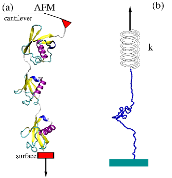
Figure 5: (a) Schematic representation of AFM technique. (b) Cartoon for the spring constant of the cantilever.

the atomic force microscopy (AFM) Binnig_PRL86 , the laser optical tweezer (LOT), magnetic tweezers , bio-membrane force probe, etc. In this section we briefly discuss the AFM which is used to probe the mechanical response of proteins under external force.

In AFM, one terminal of a biomolecules is anchored to a surface and the another one to a force sensor (Fig. 5a). The molecule is stretched by increasing the distance between the surface and the force sensor, which is a micron-sized cantilever. The force measured on experiments is proportional to the displacement of the cantilever.

If the stiffness of the cantilever $k$ is known, then a biomolecule experiences the force $f=k\delta x$, where $\delta x$ is a cantilever bending which is detected by the laser. In general, the resulting force versus extension curve is used in combination with theories for obtaining mechanical properties of biomolecules. The spring constant of AFM cantilever tip is typically $k=10-1000$ pN/nm. The value of $k$ and thermal fluctuations define spatial and force resolution in AFM experiments because when the cantilever is kept at a fixed position the force acting on the tip and the distance between the substrate and the tip fluctuate. The respective fluctuations are

$$<\delta x^{2}>=k_{B}T/k,$$ (2)

and

$$<\delta f^{2}>=kk_{B}T.$$ (3)

Here $k_{B}$ is the Boltzmann constant. For $k=10$ pN/nm and the room temperature $k_{B}T\approx 4$ pN nm we have $\sqrt{<\delta x^{2}>}\approx 0.6$ nm and $\sqrt{<\delta f^{2}>}\approx 6$ pN. Thus, AFM can probe unfolding of proteins which have unfolding force of $\sim 100$ pN, but it is not precise enough for studying, nucleic acids and molecular motors as these biomolecules have lower mechanical resistance. For these biomolecules, one can use, e.g. LOT which has the resolution $\sqrt{<\delta f^{2}}\sim 0.1$ pN.

2.4.2 Mechanical resistance of proteins

Proteins are pulled either by a constant force, $f$=const, or by a force ramped linearly with time, $f=kvt$, where $k$ is the cantilever stiffness, and $v$ is a pulling speed. In AFM experiments typical $v\sim 100$ nm/s is used Rief_Science97 . Remarkably, the force-extension curve obtained in the constant rate pulling experiments has the saw-tooth shape due to domain by domain unfolding (Fig. 6a).

Figure 6: (a) Force-extension curve obtained by stretching of a Ig8 titin fragment. Each peak corresponds to unfolding of a single domain. Smooth curves are fits to the worm-like chain model. Taken from Ref. Rief_Science97 . (b) Sketch of dependence of the force on the extension for a spring, polymer and proteins.

Here each peak corresponds to unfolding of one domain. Grubmuller et al Grubmuller_Science96 and Schulten et al Izrailev_BJ97 were first to reproduce this remarkable result by steered MD (SMD) simulations. The saw-tooth shape is not trivial if we recall that a simple spring displays the linear dependence of $f$ on extension obeying the Hooke law, while for polymers one has a monotonic dependence which may be fitted to the worm-like chain (WLC) model Marko_Macromolecules95 (Fig. 6b). A non-monotonic behavior is clearly caused by complexity of the native topology of proteins.

To characterize protein mechanical stability, one use the unfolding force $f_{u}$, which is identified as the maximum force, $f_{max}$, in the force-extension profile, $f_{u}\equiv f_{max}$. If this profile has several local maxima, then we choose the largest one. Note that $f_{u}$ depends on pulling speed logarithmically, $f_{u}\sim\ln v$ Evans_BJ97 . Most of the proteins studied so far display varying degree of mechanical resistance. Accumulated experimental and theoretical results Sulkowska_BJ08 ; MSLi_BJ07a have revealed a number of factors that govern mechanical resistance. As a consequence of the local nature of applied force, the type of secondary structural motif is thought to be important, with $\beta$-sheet structures being more mechanically resistant than all $\alpha$-helix ones MSLi_BJ07a . For example, $\beta$-protein I27 and $\alpha/\beta$-protein Ub have $f_{u}\approx 200$ pN which is considerably higher than $f_{u}\approx 30$ pN for purely $\alpha$-spectrin Rief_JMB99 . Since the secondary structure content is closely related to the contact order Plaxco_JMB98 , $f_{u}$ was shown to depend on the later linearly MSLi_BJ07a . In addition to secondary structure, tertiary structure may influence the mechanical resistance. The 24-domain ankyrin, e.g., is mechanically more stable than single- or six-domain one Lee_Nature06 . The mechanical stability depends on pulling geometry Dietz_PNAS06 . The points of application of the force to a protein and the pulling direction do matter. If a force is applied parallel to HBs (unzipping), then $\beta$-proteins are less stable than the case where the force direction is orthogonal to them (shearing). The mechanical stability can be affected by ligand binding Cao_PNAS07 and disulphide bond formation Wiita_Nature07 . Finally, note that the mechanical resistance of proteins can be captured not only by all-atom SMD Sotomayor_Science07 , but also by simple Go models Sulkowska_BJ08 ; MSLi_BJ07a . This is because the mechanical unfolding is mainly governed by the native topology and native topology-based Go models suffice. However, in this thesis, we will show that in some cases non-native interactions can not be neglected.

2.4.3 Construction of unfolding free energy landscape by SMFS

Deciphering FEL is a difficult task as it is a function of many variables. Usually, one projects it into one- or two-dimensional space. The validity of such approximate mapping is not a priory clear and experiments should be used to justify this. In the mechanical unfolding case, however, the end-to-end extension $\Delta R$ can serve as a good reaction coordinate and FEL can be mapped into this dimension. Thus, considering FEL as a function of $\Delta R$, one can estimate the distance between the NS and TS, $x_{u}$, using either the dependencies of unfolding rates on the external force MSLi_BJ07 or the dependencies of $f$ on pulling speed $v$ Carrion-Vasquez_PNAS99 . Unfolding barriers may be also extracted with the help of the non-linear kinetic theory Dudko_PRL06 (see below).

Experiments and simulations MSLi_BJ07a showed that $x_{u}$ varies between 2 - 15 Å, depending on the secondary structure content or the contact order. The smaller CO , the larger is $x_{u}$. It is remarkable that $x_{u}$ and unfolding force $f_{u}$ are mutually related. Namely, using a simple network model, Dietz and Rief Dietz_PRL08 argued that $x_{u}f_{u}$ $\approx$ 50 pN nm for many proteins.

Chapter 3 Modeling, Computational tools and theoretical background

3.1 Modeling of Proteins

In this section we briefly discuss main models used to study protein dynamics.

3.1.1 Lattice models

In last about fifteen years, considerable insight into thermodynamics and kinetics of protein folding has been gained due to simple lattice models Dill_ProteinSci95 ; Kolinski_book96 . Here amino acids are represented by single beads which are located at vertices of a cubic lattice. The most important difference from homopolymer models is that amino acid sequences and the role of contacts should be taken into account. Due to the constraint that a contact is formed if two residues are nearest neighbors, but not successive in sequence, a contacts between residues $i$ and $j$ is allowed provided $|i-j|\geq 3$. In the simple Go modeling Go_ARBB83 , the interaction between two beads which form a native contact is assumed to be attractive, while the non-native interaction is repulsive. This energy choice guarantees that the native conformation has the lowest energy. In more realistic models specific interactions between amino acids are taken into account. Several kinds of potentials Miyazawa_Macromolecules85 ; Kolinski_JCP93 ; Betancourt_ProSci99 are used to describe these interactions.

A next natural step to mimic more realistic features of proteins such as a dense core packing is to include the rotamer degrees of freedom Kolinski_Proteins96 . One of the simplest models is a cubic lattice of a backbone sequence of $N$ beads, to which a side bead representing a side chain is attached Bromberg_ProteinSci94 (Fig. 7). The system has in total 2$N$ beads. Here we consider a Go model, where the energy of a conformation is Kouza_JPCA06

$$E\;=\;\epsilon_{bb}\sum_{i=1,j>i+1}^{N}\,\delta_{r_{ij}^{bb},a}+\epsilon_{bs}\sum_{i=1,j\neq i}^{N}\,\delta_{r_{ij}^{bs},a}+\epsilon_{ss}\sum_{i=1,j>i}^{N}\,\delta_{r_{ij}^{ss},a}\;,$$ (4)

where $\epsilon_{bb},\epsilon_{bs}$ and $\epsilon_{ss}$ are backbone-backbone(BB-BB), backbone-side chain (BB-SC) and side chain-side chain (SC-SC) contact energies, respectively. The distances $r_{ij}^{bb},r_{ij}^{bs}$ and $r_{ij}^{ss}$ are between BB, BS and SS beads, respectively. The contact energies $\epsilon_{bb},\epsilon_{bs}$ and $\epsilon_{ss}$ are taken to be -1 (in units of k_bT) for native and 0 for non-native interactions. The neglect of interactions between residues not present in the NS is the approximation used in the Go model.

In order to monitor protein dynamics usually one use the standard move set which includes the tail flip, corner flip, and crankshaft for backbone beads. The Metropolis criterion is applied to accept or reject moves Kolinski_book96 . While lattice models have been widely used in the protein folding problem Kolinski_book96 , they attract little attention in the mechanical unfolding simulation Socci_PNAS99 . In present thesis, we employed this model to study the cooperativity of the folding-unfolding transition.

Figure 7: Representation of protein conformation by lattice model with side chain (a), off-lattice C_α-Go model (b) and all-atom model (c).

3.1.2 Off-lattice coarse-grained Go modeling

The major shortcoming of lattice models is that beads are confined to lattice vertices and it does not allow for describing the protein shape accurately. This can be remedied with the help of off-lattice models in which beads representing amino acids can occupy any positions (Fig. 7b). A number of off-lattice coarse-grained models with realistic interactions (not Go) between amino acids have been developed to study the mechanical resistance of proteins Klimov_PNAS00 ; Kirmizialtin_JCP05 . However, it is not an easy task to construct such models for long proteins.

In the pioneer paper Go_ARBB83 Go introduced a very simple model in which non-native interactions are ignored. This native topology-based model turns out to be highly useful in predicting the folding mechanisms and deciphering the free energy landscapes of two-state proteins Takaga_PNAS99 ; Clementi_JMB00 ; Koga_JMB01 . On the other hand, in mechanically unfolding one stretches a protein from its native conformation, unfolding properties are mainly governed by its native topology. Therefore, the native-topology-based or Go modeling is suitable for studying the mechanical unfolding. Various versions of Go models Clementi_JMB00 ; Cieplak_Proteins02 ; Karanicolas_ProSci02 ; West_BJ06 ; Hyeon_Structure06 ; MSLi_BJ07 have been applied to this problem. In this thesis we will focus on the variant of Clementi et al. Clementi_JMB00 . Here one uses coarse-grained continuum representation for a protein in which only the positions of C_α-carbons are retained. The interactions between residues are assumed to be Go-like and the energy of such a model is as follows Clementi_JMB00

$$E\; = \;\sum_{bonds}K_{r}(r_{i}-r_{0i})^{2}+\sum_{angles}K_{\theta}(\theta_{i}-\theta_{0i})^{2}$$ (5)

$$+ \sum_{dihedral}\{K_{\phi}^{(1)}[1-\cos(\phi_{i}-\phi_{0i})]+K_{\phi}^{(3)}[1-\cos 3(\phi_{i}-\phi_{0i})]\}$$

$$+ \sum_{i>j-3}^{NC}\epsilon_{H}\left[5\left(\frac{r_{0ij}}{r_{ij}}\right)^{12}-6\left(\frac{r_{0ij}}{r_{ij}}\right)^{10}\right]+\sum_{i>j-3}^{NNC}\epsilon_{H}\left(\frac{C}{r_{ij}}\right)^{12}+E_{f}.$$

Here $\Delta\phi_{i}=\phi_{i}-\phi_{0i}$, $r_{i,i+1}$ is the distance between beads $i$ and $i+1$, $\theta_{i}$ is the bond angle between bonds $(i-1)$ and $i$, and $\phi_{i}$ is the dihedral angle around the $i$th bond and $r_{ij}$ is the distance between the $i$th and $j$th residues. Subscripts “0”, “NC” and “NNC” refer to the native conformation, native contacts and non-native contacts, respectively. Residues $i$ and $j$ are in native contact if $r_{0ij}$ is less than a cutoff distance $d_{c}$ taken to be $d_{c}=6.5$ Å, where $r_{0ij}$ is the distance between the residues in the native conformation.

The local interaction in Eq. (5) involves three first terms. The harmonic term accounts for chain connectivity (Fig. 8a), while the second term represents the bond angle potential (Fig. 8b). The potential for the dihedral angle degrees of freedom (Fig. 8c) is given by the third term in Eq. (5). The non-local interaction energy between residues that are separated by at least 3 beads is given by 10-12 Lennard-Jones potential (Fig. 8e). A soft sphere repulsive potential (the fifth term in Eq. 5) disfavors the formation of non-native contacts. The last term accounts for the force applied to C and N termini along the end-to-end vector $\vec{R}$. We choose $K_{r}=100\epsilon_{H}/\AA^{2}$, $K_{\theta}=20\epsilon_{H}/rad^{2},K_{\phi}^{(1)}=\epsilon_{H}$, and $K_{\phi}^{(3)}=0.5\epsilon_{H}$, where $\epsilon_{H}$ is the characteristic hydrogen bond energy and $C=4$ Å.

Figure 8: Schematic representation for covalent bonding (a), bond angle interactions (b), proper torsion potential (c), improper dihedral angles (d), long range Van der Waals (e) and electrostatic interactions (f).

In the constant force simulations the last term in Eq. (5) is

$$E_{f}\;=\;-\vec{f}.\vec{r},$$ (6)

where $\vec{r}$ is the end-to-end vector and $\vec{f}$ is the force applied either to both termini or to one of them. In the constant velocity force simulation we fix the N-terminal and pull the C-terminal by force

$$f\;=\;k(vt-x),$$ (7)

where $x$ is the displacement of the pulled atom from its original position Lu_BJ98 , and the pulling direction was chosen along the vector from fixed atom to pulled atom. In order to mimic AFM experiments (see section Experimental technique), throughout this thesis we used the $k=K_{r}=100\epsilon_{H}/\AA^{2}\;\approx 100$ pN/nm, which has the same order of magnitude as those for cantilever stiffness.

3.1.3 All-atom models

The intensive theoretical study of protein folding has been performed with the help of all-atom simulations Isralewitz_COSB01 ; Gao_PCCP06 ; Sotomayor_Science07 . All-atom models include the local interaction and the non-bonded terms. The later include the (6-12) Lenard-Jones potential, the electro-static interaction, and the interaction with environment. The all-atom model with the CHARMM force field Brooks_JCC83 and explicit TIP3 water Jorgenson_JCP83 has been employed first by Grubmuller et al. Grubmuller_Science96 to compute the rupture force of the streptavidin-biovitin complex. Two years later a similar model was successfully applied by Schulten and coworkers Lu_BJ98 to the titin domain I27. The NAMD software Phillips_JCC05 developed by this group is now widely used for stretching biomolecules by the constant mechanical force and by the force with constant loading rate (see recent review Isralewitz_COSB01 for more references). NAMD works with not only CHARMM but also with AMBER potential parameters Weiner_JCC81 , and file formats. Recently, it becomes possible to use the GROMACS software Gunstren_96 for all-atom simulations of mechanical unfolding of proteins in explicit water. As we will present results obtained for mechanical unfolding of DDFLN4 using the Gromacs software, we discuss it in more detail.

Gromacs force field we use provides parameters for all atoms in a system, including water molecules and hydrogen atoms. The general functional form of a force filed consists of two terms:

$$E_{total}=E_{bonded}+E_{nonbonded}$$ (8)

where $E_{bonded}$ is the bonded term which is related to atoms that are linked by covalent bonds and $E_{nonbonded}$ is the nonbonded one which is described the long-range electrostatic and van der Waals forces.

Bonded interactions. The potential function for bonded interactions can be subdivided into four parts: covalent bond-stretching, angle-bending, improper dihedrals and proper dihedrals. The bond stretching between two covalently bonded atoms $i$ and $j$ is represented by a harmonic potential

$$V_{b}(r_{ij})=\frac{1}{2}k_{ij}^{b}(r_{ij}-b_{ij})^{2}$$ (9)

where $r_{ij}$ is the actual bond length, $b_{ij}$ the reference bond lengh, $k_{ij}$ the bond stretching force constant. Both reference bond lengths and force constants are specific for each pair of bound atoms and they are usually extracted from experimental data or from quantum mechanical calculations.

The bond angle bending interactions between a triplet of atoms i-j-k are also represented by a harmonic potential on the angle $\theta_{ijk}$

$$V_{a}(\theta_{ijk})=\frac{1}{2}k_{ijk}^{\theta}(\theta_{ijk}-\theta_{ijk}^{0})^{2}$$ (10)

where $k_{ijk}^{\theta}$ is the angle bending force constant, $\theta_{ijk}$ and $\theta_{ijk}^{0}$ are the actual and reference angles, respectively. Values of $k_{ijk}^{\theta}$ and $\theta_{ijk}^{0}$ depend on chemical type of atoms.

Proper dihedral angles are defined according to the IUPAC/IUB convention (Fig. 8c), where $\phi$ is the angle between the ijk and the ikl planes, with zero corresponding to the cis configuration (i and l on the same side). To mimic rotation barriers around the bond the periodic cosine form of potential is used.

$$V_{d}(\phi_{ijkl})=k_{\phi}(1+cos(n\phi-\phi_{s}))$$ (11)

where $k_{\phi}$ is dihedral angle force constant, $\phi_{s}$ is the dihedral angle (Fig. 8c), and $n$=1,2,3 is a coefficient of symmetry.

Improper potential is used to maintain planarity in a molecular structure. The torsional angle definition is shown in the figure 8d. The angle $\xi_{ijkl}$ still depends on the same two planes ijk and jkl, as can be seen in the figure with the atom i in the center instead on one of the ends of the dihedral chain. Since this potential used to maintain planarity, it only has one minimum and a harmonic potential can be used:

$$V_{id}(\xi_{ijkl})=\frac{1}{2}k_{\xi}(\xi_{ijkl}-\xi_{0})^{2}$$ (12)

where $k_{\xi}$ is improper dihedral angle bending force constant, $\xi_{ijkl}$ - improper dihedral angle.

Nonbonded interactions. They act between atoms within the same protein as well as between different molecules in large protein complexes. Non bonded interactions are divided into two parts: electrostatic (Fig. 8f) and Van der Waals (Fig. 8e) interactions. The electrostatic interactions are modeled by Coulomb potential:

$$V_{c}(r_{ij})=\frac{q_{i}q_{j}}{4\pi\epsilon_{0}r_{ij}}$$ (13)

where $q_{i}$ and $q_{j}$ are atomic charges, $r_{ij}$ distance between atoms i and j, $\epsilon_{0}$ the electrical permittivity of space. The interactions between two uncharged atoms are described by the Lennard-Jones potential

$$V_{LJ}(r_{ij})=\frac{C_{ij}^{12}}{r_{ij}^{12}}-\frac{C_{ij}^{6}}{r_{ij}^{6}}$$ (14)

where $C_{ij}^{12}$ and $C_{ij}^{6}$ are specific Lennard-Jones parameters which depend on pairs of atom types.

SPC water model. To calculate the interactions between molecules in solvent, we use a model of the individual water molecules what tell us where the charges reside. Gromacs software uses SPC or Simple Charge Model to represent water molecules. The water molecule has three centers of concentrated charge: the partial positive charges on the hydrogen atoms are balanced by an appropriately negative charge located on the oxygen atom. An oxygen atom also gets the Lennard-Jones parameters for computing intermolecular interactions between different molecules. Van der Waals interactions involving hydrogen atoms are not calculated.

3.2 Molecular Dynamics

One of the important tools that have been employed to study the biomolecules are the molecular dynamics (MD) simulations. It was first introduced by Alder and Wainwright in 1957 to study the interaction of hard spheres. In 1977, the first biomolecules, the bovine pancreatic trypsin inhibitor (BPTI) protein, was simulated using this technique. Nowadays, the MD technique is quite common in the study of biomolecules such as solvated proteins, protein-DNA complexes as well as lipid systems addressing a variety of issues including the thermodynamics of ligand-binding, the folding and unfolding of proteins.

It is important to note that biomolecules exhibit a wide range of time scales over which specific processes take place. For example, local motion which involves atomic fluctuation, side chain motion, and loop motion occurs in the length scale of 0.01 to 5 Å and the time involved in such process is of the order of 10^-15 to 10^-12 s. The motion of a helix, protein domain or subunit falls under the rigid body motion whose typical length scales are in between 1 – 10 Å and time involved in such motion is in between 10^-9 to $10^{-6}$ s. Large-scale motion consists of helix-coil transitions or folding unfolding transition, which is more than 5 Å and time involved is about 10^-7 to 10¹ s. Typical time scales for protein folding are 10^-6 to 10¹ s Kubelka_COSB04 . In unfolding experiments, to stretch out a protein of length $10^{2}$ nm, one needs time $\sim$ 1 s using a pulling speed $v\sim 10^{2}$ nm/s Rief_Science97 .

The steered MD (SMD) that combines the stretching condition with the standard MD was initiated by Schulten and coworkers Isralewitz_COSB01 . They simulated the force-unfolding of a number of proteins showing atomic details of the molecular motion under force. The focus was on the rupture events of HBs that stabilized the structures. The structural and energetic analysis enabled them to identify the origin of free energy barrier and intermediates during mechanical unfolding. However, one has to notice that there is enormous difference between the simulation condition used in SMD and real experiment. In order to stretch out proteins within a reasonable amount of CPU time, SMD simulations at constant pulling speed use eight to ten orders of higher pulling speed, and one to two orders of larger spring constant than those of AFM experiments. Therefore, effective force acting on the molecule is about three-four orders higher. It is unlikely, that the dynamics under such an extreme condition can mimic real experiments, and one has to be very careful about comparison of simulation results with experimental ones. In literature the word ”steered” also means MD at extreme conditions, where constant force and constant pulling speed are chosen very high.

Excellent reviews on MD and its use in biochemistry and biophysics are numerous (see, e.g., Adcock_ChemRev06 and references therein). Below, we only focus on the Brownian dynamics as well as on the second-order Verlet method for the Langevin dynamics simulation , which have been intensively used to obtain main results presented in this thesis.

3.2.1 Langevin dynamics simulation

The Langevin equation is a stochastic differential equation which introduces friction and noise terms into Newton’s second law to approximate effects of temperature and environment:

$$m\frac{d^{2}\vec{r}}{dt^{2}}=\vec{F}_{c}-\gamma\frac{d\vec{r}}{dt}+\vec{\Gamma}\equiv\vec{F}.$$ (15)

where $\Gamma$ is a random force, $m$ the mass of a bead, $\gamma$ the friction coefficient, and $\vec{F}_{c}=-d\vec{E}/d\vec{r}$. Here the configuration energy $E$ for the Go model, for example, is given by Eq. (5). The random force $\Gamma$ is taken to be a Gaussian random variable with white noise spectrum and is related to the friction coefficient by the fluctuation-dissipation relation:

$$<\Gamma(t)\Gamma(t^{\prime})>=2\gamma k_{B}T\delta(t-t^{\prime})$$ (16)

where $k_{B}$ is a Boltzmann’s constant, $\gamma$ friction coefficient, $T$ temperature and $\delta(t-t^{\prime})$ the Dirac delta function. The friction term only influences kinetic but not thermodynamic properties.

In the low friction regime, where $\gamma<25\frac{m}{\tau_{L}}$ (the time unit $\tau_{L}=(ma^{2}/\epsilon_{H})^{1/2}\approx 3$ ps), Eq. (15) can be solved using the second-order Velocity Verlet algorithm Swope_JCP82 :

$$x(t+\Delta t)\;=\;x(t)+\dot{x}(t)\Delta t+\frac{1}{2m}F(t)(\Delta t)^{2},$$ (17)

$$\dot{x}(t+\Delta t)\;=\;\left(1-\frac{\gamma\Delta t}{2m}\right)\left[1-\frac{\gamma\Delta t}{2m}+\left(\frac{\gamma\Delta t}{2m}\right)^{2}\right]\dot{x}(t)+\qquad$$

$$\left(1-\frac{\gamma\Delta t}{2m}+\left(\frac{\gamma\Delta t}{2m}\right)^{2}\right)(F_{c}(t)+\Gamma(t)+F_{c}(t+\Delta t)+\Gamma(t+\Delta t))\frac{\Delta t}{2m}+o(\Delta t^{2}),$$ (18)

with the time step $\Delta t=0.005\tau_{L}$.

3.2.2 Brownian dynamics

In the overdamped limit ($\gamma>25\frac{m}{\tau_{L}}$) the inertia term can be neglected, and we obtain a much simpler equation:

$$\frac{dr}{dt}=\frac{1}{\gamma}(F_{c}+\Gamma).$$ (19)

This equation may be solved using the simple Euler method which gives the position of a biomolecule at the time $t+\Delta t$ as follows:

$$x(\Delta t+t)=x(t)+\frac{\Delta t}{\gamma}(F_{c}+\Gamma).$$ (20)

Due to the large value of $\gamma$ we can choose the time step $\Delta t=0.1\tau_{L}$ which is 20-fold larger than the low viscosity case. Since the water has $\gamma\approx 50\frac{m}{\tau_{L}}$ Veitshans_FD97 , the Euler method is valid for studying protein dynamics.

3.3 Theoretical background

In this section we present basic formulas used throughout my thesis.

3.3.1 Cooperativity of folding-unfolding transition

The sharpness of the fold-unfolded transition might be characterized quantitatively via the cooperativity index $\Omega_{c}$ which is defined as follows MSLi_Polymer04

$$\Omega_{c}=\frac{T_{F}^{2}}{\Delta T}\biggl{(}\frac{df_{N}}{dT}\biggr{)}_{T=T_{F}},$$ (21)

where $\Delta T$ is the transition width and $f_{N}$ the probability of being in the NS. The larger $\Omega_{c}$, the sharper is the transition. $f_{N}$ is defined as the thermodynamic average of the fraction of native contacts $\chi$, $f_{N}=<\chi>$. For off-lattice models, $\chi$ is Camacho_PNAS93 :

$$\chi\;=\frac{1}{Q_{total}}\sum_{i<j+1}^{N}\,\;\theta(1.2r_{0ij}-r_{ij})\Delta_{ij}$$ (22)

where $\Delta_{ij}$ is equal to 1 if residues $i$ and $j$ form a native contact and 0 otherwise and $\theta(x)$ is the Heaviside function. The argument of this function guarantees that a native contact between $i$ and $j$ is classified as formed when $r_{ij}$ is shorter than 1.2$r_{0ij}$ Clementi_JMB00 . In the lattice model with side chain (LMSC) case, we have

$$\chi\;=\;\frac{1}{2N^{2}-3N+1}\left[\sum_{i<j}\,\delta(r_{ij}^{ss}-r_{ij}^{ss,N})+\sum_{i<j+1}\,\delta(r_{ij}^{bb}-r_{ij}^{bb,N})+\sum_{i\neq j}\,\delta(r_{ij}^{bs}-r_{ij}^{bs,N})\;\right].$$ (23)

Here $bb$, $bs$ and $ss$ refer to backbone-backbone, backbone-side chain and side chain-side chain pairs, respectively.

3.3.2 Kinetic theory for mechanical unfolding of biomolecules

One of the notable aspects in force experiments on single biomolecules is that the end-to-end extension $\Delta R$ is directly measurable or controlled by instrumentation. $\Delta R$ becomes a natural reaction coordinate for describing mechanical processes.

The theoretical framework for understanding the effect of external constant force on rupture rates was first discussed in the context of cell-cell adhesion by Bell in 1978 Bell_Sci78 . Evans and Rirchie have extended his theory to the case when the loading force increases linearly with time Evans_BJ97 . The phenomenological Bell theory is based on the assumption that the TS does not move under stretching. Since this assumption is not true, Dudko et al Dudko_PRL06 have developed the microscopic theory which is free from this shortcoming. In this section we discuss the phenomenological as well as microscopic kinetics theory.

Bell theory for constant force case.

Suppose the external constant force, $f$, is applied to the termini of a biomolecule. The deformation of the FEL under force is schematically shown in Fig. 9. Assuming that the force does not change the distance between the NS and TS ($x_{u}(f)=x_{u}(0)$), Bell Bell_Sci78 stated that the activation energy is changed to $\Delta G^{{\ddagger}}_{u}(f)=\Delta G^{{\ddagger}}_{u}(0)-fx_{u}$, where $x_{u}=x_{u}(0)$. In general, the proportionality factor $x_{u}$ has the dimension of length and may be viewed as the width of the potential. Using the Arrhenius law, Bell obtained the following formula for the unfolding/unbinding rate constant Kramers_Physica40 :

$$k_{u}(f)\;=\;k_{u}(0)\exp(fx_{u}/k_{B}T),$$ (24)

where $k_{u}(0)$ is the rate constant is the unfolding rate constant in the absence of a force. If a reaction takes place in condensed phase, then according to the Kramers theory the prefactor $k_{u}(0)$ is equal

$$k_{u}(0)\;=\;\frac{\omega_{0}\omega_{ts}}{2\pi\gamma}\exp(-\Delta G^{{\ddagger}}_{u}(0)/k_{B}T).$$ (25)

Here $\gamma$ is a solvent viscosity, $\omega_{0}$ the angular frequency (curvature) at the reactant bottom, and $\omega_{ts}$ the curvature at barrier top of the effective reaction coordinate Kramers_Physica40 . For biological reactions, which belong to the Kramers category, $\frac{\omega_{0}\omega_{ts}}{2\pi\gamma}\sim 1\mu$s Levinthal_JCP68 .

Figure 9: Conceptual plot for the FEL without (blue) and under (red) the external force. $x_{u}$ is the shift of $x_{u}$ in the presence of force.

It is important to note that the unfolding rate grows exponentially with the force. This is the hallmark of the Bell model. Even Eq. (24) is very simple, as we will see below, it fits most of experimental data very well. Using Eq. (24), one can extract the distance $x_{u}$, or the location of the TS.

Bell theory for force ramp case.

Assuming that the force increases linearly with a rate $v$, Evans and Rirchie in their seminal paper Evans_BJ97 , have shown that the distribution of unfolding force $P(f)$ obeys the following equation:

$$P(f)\;=\;\frac{k_{u}(f)}{v}\exp\{\frac{k_{B}T}{x_{u}v}\left[k_{u}(0)-k_{u}(f)\right]\},$$ (26)

where $k_{u}(f)$ is given by Eq. (24). Then, the most probable unbinding force or the maximum of force distribution $f_{max}$, obtained from the condition $dP(f)/df|_{f=f_{max}}=0$, is

$$f_{max}=\frac{k_{B}T}{x_{u}}ln\frac{kvx_{u}}{k_{u}(0)k_{B}T}.$$ (27)

The logarithmic dependence of $f_{max}$ on the pulling speed $v$ was confirmed by enumerous experiments and simulations Klimov_PNAS99 ; Kouza_JCP08 .

Beyond Bell approximation.

The major shortcoming of the the Bell approximation is the assumption that $x_{u}$ does not depend on the external force. Upon force application the location of TS should move closer to the NS reducing $x_{u}$ (Fig 9), as postulated by Hammond in the context of chemical reactions of small organic molecules Hammond_JACS53 . The Hammond behavior has been observed in protein folding experiments Matouschek_Biochemistry95 and simulations Lacks_BJ05 .

Recently, assuming that $x_{u}$ depends on the external force and using the Kramers theory, several groups Schlierf_BJ06 ; Dudko_PRL06 have tried to go beyond the Bell approximation. We follow Dudko et al. who proposed the following force dependence for the unfolding time Dudko_PRL06 :

$$\tau_{u}\;=\;\tau_{u}^{0}\left(1-\frac{\nu x_{u}}{\Delta G^{\ddagger}}\right)^{1-1/\nu}\exp\{-\frac{\Delta G^{\ddagger}}{k_{B}T}[1-(1-\nu x_{u}f/\Delta G^{\ddagger})^{1/\nu}]\}.$$ (28)

Here, $\Delta G^{\ddagger}$ is the unfolding barrier, and $\nu=1/2$ and 2/3 for the cusp Hummer_BJ03 and the linear-cubic free energy surface Dudko_PNAS03 , respectively. Note that $\nu=1$ corresponds to the phenomenological Bell theory (Eq. 24), where $\tau_{u}=1/k_{u}$. An important consequence following from Eq. (28), is that one can apply it to estimate not only $x_{u}$, but also $\Delta G^{\ddagger}$, if $\nu\neq 1$. Expressions for the distribution of unfolding forces and the $f_{max}$ for arbitrary $\nu$ may be found in Dudko_PRL06 .

3.3.3 Kinetic theory for refolding of biomolecules.

In force-clamp experiments Fernandez_Sci04 , a protein refolds under the quenched force. Then, in the Bell approximation, the external force increases the folding barrier (see Fig. 9) by amount $\Delta G^{{\ddagger}}_{f}=fx_{f}$, where $x_{f}=x_{f}(0)$ is a distance between the DS and the TS. Therefore, the refolding time reads as

$$\tau_{f}(f)\;=\;\tau_{f}(0)\exp(fx_{f}/k_{B}T).$$ (29)

Using this equation and the force dependence of $\tau_{f}(f)$, one can extract $x_{f}$ Fernandez_Sci04 ; MSLi_PNAS06 ; MSLi_BJ07 . One can extend the nonlinear theory of Dudko et al Dudko_PRL06 to the refolding case by replacing $x_{u}\rightarrow-x_{f}$ in, e.g., Eq. (28). Then the folding barriers can be estimated using the microscopy theory with $\nu\neq 1$.

3.4 Progressive variable

In order to probe folding/refolding pathways, for $i$-th trajectory we introduce the progressive variable

$$\delta_{i}=t/\tau^{i}_{f}.$$ (30)

Here $\tau^{i}_{f}$ is the folding time, which is is defined as a time to get the NS starting from the denaturated one for the $i$-th trajectory. Then one can average the fraction of native contacts over many trajectories in a unique time window $0\leq\delta_{i}\leq 1$ and monitor the folding sequencing with the help of the progressive variable $\delta$.

In the case of unfolding, the progressive variable is defined in a similar way:

$$\delta_{i}=t/\tau^{i}_{u}.$$ (31)

Here $\tau^{i}_{u}$ is the folding time, which is is defined as a time to get a rod conformation starting from the NS for the $i$-th trajectory. The unfolding time, $\tau_{u}$, is the average of first passage times to reach a rod conformation. Different trajectories start from the same native conformation but, with different random number seeds. In order to get the reasonable estimate for $\tau_{u}$, for each case we have generated 30 - 50 trajectories. Unfolding pathways were probed by monitoring the fraction of native contacts of secondary structures as a function of progressive variable $\delta$.

Chapter 4 Effect of finite size on cooperativity and rates of protein folding

4.1 Introduction

Single domain globular proteins are mesoscopic systems that self-assemble, under folding conditions, to a compact state with definite topology. Given that the folded states of proteins are only on the order of tens of Angstroms (the radius of gyration $R_{g}\approx 3N^{\frac{1}{3}}$ Å  Dima_JPCB04 where $N$ is the number of amino acids) it is surprising that they undergo highly cooperative transitions from an ensemble of unfolded states to the NS Privalov_APC79 . Similarly, there is a wide spread in the folding times as well Galzitskaya_Proteins03 . The rates of folding vary by nearly nine orders of magnitude. Sometime ago it was shown theoretically that the folding time ,$\tau_{F}$, should depend on $N$ Finkelstein_FoldDes97 but only recently has experimental data confirmed this prediction Galzitskaya_Proteins03 ; MSLi_Polymer04 ; Ivankov_PNAS04 . It has been shown that $\tau_{F}$ can be approximately evaluated using $\tau_{F}\approx\tau_{F}^{0}\exp(N^{\beta})$ where $1/2\leq\beta<2/3$ with the prefactor $\tau_{F}^{0}$ being on the order of a $\mu s$.

Much less attention has been paid to finite size effects on the cooperativity of transition from unfolded states to the native basin of attraction (NBA). Because $N$ is finite, large conformational fluctuations are possible but require careful examination Klimov_JCC02 ; MSLi_Polymer04 . For large enough $N$ it is likely that the folding or melting temperature itself may not be unique Holtzer_BJ97 . Although substantial variations in $T_{m}$ are unlikely it has already been shown that the there is a range of temperatures over which individual residues in a protein achieve their NS ordering Holtzer_BJ97 . On the other hand, the global cooperativity, as measured by the dimensionless parameter $\Omega_{c}$ (Eq. 21) has been shown to scale as MSLi_PRL04

$$\Omega_{c}\approx N^{\zeta}$$ (32)

Having used the scaling arguments and analogy with a magnetic system, it was shown that MSLi_PRL04

$$\zeta=1+\gamma\approx 2.2$$ (33)

where the magnetic susceptibility exponent $\gamma\approx 1.2$. This result in not trivial because the protein melting transition is first order Privalov_APC79 , for which $\zeta=2$ Naganathan_JACS05 . Let us mention the main steps leading to Eq. (33). The folding temperature can be identified with the peak in $d<\chi>/dT$ or in the fluctuations in $\chi$, namely, $\Delta\chi=<\chi^{2}>-<\chi>^{2}$. Using an analogy to magnetic systems, we identify $T(\partial<\chi>/\partial h)=\Delta\chi$ where $h$ is an ”ordering field” that is conjugate to $\chi$. Since $\Delta\chi$ is dimensionless, we expect $h\approx T$ for proteins, and hence, $T(\partial<\chi>/\partial T)$ is like susceptibility. Hence, the scaling of $\Omega_{c}$ on $N$ should follow the way $(T_{F}/\Delta T)\Delta\chi$ changes with $N$ Kohn_PNAS04 .

For efficient folding in proteins $T_{F}\approx T_{\Theta}$ Klimov_PRL97 , where $T_{\Theta}$ is the temperature at which the coil-globule transition occurs. It has been argued that $T_{F}$ for proteins may well be a tricritical point, because the transition at $T_{F}$ is first-order while the collapse transition is (typically) second-order. Then, as temperature approaches from above, we expect that the characteristics of polypeptide chain at $T_{\Theta}$ should manifest themselves in the folding cooperativity. At or above $T_{F}$, the susceptibility $\Delta\chi$ should scales with $\Delta T$ as $\Delta\chi\sim\Delta T^{-\gamma}$ as predicted by the scaling theory for second order transitions Fisher_PRB82 . Therefore, $\Omega_{c}\sim\Delta T^{-(1+\gamma)}$. taking into account that $\Delta T\sim N^{-1}$ Grosberg_Book94 we come to Eqs. 32 and 33.

In this chapter we use LMSC, off-lattice Go models for 23 proteins and experimental results for a number of proteins to further confirm the theoretical predictions (Eq. 32 and 33). Our results show that $\zeta\approx 2.22$ which is distinct from the expected result ($\zeta=2.0$) for a strong first order transition Fisher_PRB82 . Our another goal is to study the dependence of the folding time on the number of amino acids. The larger data set of proteins for which folding rates are available shows that the folding time scales as

$$\tau_{F}=\tau_{0}\exp(cN^{\beta})$$ (34)

with $c\approx 1.1$, $\beta=1/2$ and $\tau_{0}\approx 0.2\mu s$.

The results presented in this chapter are taken from Ref. Kouza_JPCA06 .

4.2 Models and methods

The LMSC (Eq. 4) and coarse-grained off-lattice model (Eq. 5) Clementi_JMB00 were used. For the LMSC we performed Monte Carlo simulations using the previously well-tested move set MS3 Li_JPCB02 . This move set ensures that ergodicity is obtained efficiently even for $N=50$, it uses single, double and triple bead moves Betancourt_JCP98 . Following standard practice the thermodynamic properties are computed using the multiple histogram method Ferrenberg_PRL89 . The kinetic simulations are carried out by a quench from high temperature to a temperature at which the NBA is preferentially populated. The folding times are calculated from the distribution of first passage times.

For off-lattice models, we assume the dynamics of the polypeptide chain obeys the Langevin equation. The equations of motion were integrated using the velocity form of the Verlet algorithm with the time step $\Delta t=0.005\tau_{L}$, where $\tau_{L}=(ma^{2}/\epsilon_{H})^{1/2}\approx 3$ ps. In order to calculate the thermodynamic quantities we collected histograms for the energy and native contacts at five or six different temperatures (at each temperature 20 - 50 trajectories were generated depending on proteins). As with the LMSC we used the multiple histogram method Ferrenberg_PRL89 to obtain the thermodynamic parameters at all temperatures. For off-lattice and LMSC models the probability of being in the NS is computed using Eq. (22) and Eq. (23), respectively.

The extent of cooperativity of the transition to the NBA from the ensemble of unfolded states is measured using the dimensionless parameter $\Omega_{c}$ (Eq. 21). Two points about $\Omega_{c}$ are noteworthy. (1) For proteins that melt by a two-state transition it is trivial to show that $\Delta H_{vH}=4k_{B}\Delta T\Omega_{c}$, where $\Delta H_{vH}$ is the van’t Hoff enthalpy at $T_{F}$. For an infinitely sharp two-state transition there is a latent heat release at $T_{F}$, at which $C_{p}$ can be approximated by a delta-function. In this case $\Omega_{c}\rightarrow\infty$ which implies that $\Delta H_{vH}$ and the calorimetric enthalpy $\Delta H_{cal}$ (obtained by integrating the temperature dependence of the specific heat $C_{p}$ ) would coincide. It is logical to infer that as $\Omega_{c}$ increases the ratio $\kappa=\Delta H_{vH}/\Delta H_{cal}$ should approach unity. (2) Even for moderate sized proteins that undergo a two-state transition $\kappa\approx 1$ Privalov_APC79 . It is known that the extent of cooperativity depends on external conditions as has been demonstrated for thermal denaturation of CI2 at several values of pH Jackson_Biochemistry91 . The values of $\kappa$ for all pH values are $\approx 1$. However, the variation in cooperativity of CI2 as pH varies are reflected in the changes in $\Omega_{c}$ Klimov_FD98 . Therefore, we believe that $\Omega_{c}$, that varies in the range $0<\Omega_{c}<\infty$, is a better descriptor of the extent of cooperativity than $\kappa$. The latter merely tests the applicability of the two-state approximation.

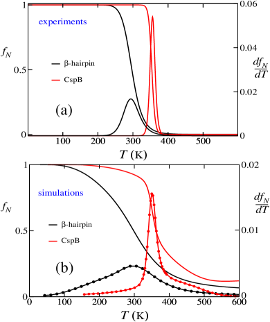
Figure 10: The temperature dependence of $f_{N}$ and $df_{N}/dT$ for $\beta$-hairpin ($N=16$) and CpsB ($N=67$). The scale for $df_{N}/dT$ is given on the right. (a): the experimental curves were obtained using $\Delta H=11.6$ kcal/mol, $T_{m}=297$ K and $\Delta H=54.4$ kcal/mol and $T_{m}=354.5$ K for $\beta$-hairpin and CpsB, respectively. (b): the simulation results were calculated from $f_{N}=<\chi(T)>$. The Go model gives only a qualitatively reliable estimates of $f_{N}(T)$.

4.3 Results

4.3.1 Dependence of cooperativity $\Omega_{c}$ on number of aminoacids $N$

For the 23 Go proteins listed in Table 1, we calculated $\Omega_{c}$ from the temperature dependence of $f_{N}$. In Fig. 10 we compare the temperature dependence of $f_{N}(T)$ and $df_{N}(T)/dT$ for $\beta$-hairpin ($N=16$) and Bacillus subtilis (CpsB, $N=67$). It is clear that the transition width and the amplitudes of $df_{N}/dT$ obtained using Go models, compare only qualitatively well with experiments. As pointed out by Kaya and Chan Kaya_SFG00 ; Kaya_JMB03 ; Chan_ME04 ; Kaya_PRL00 , the simple Go-like models consistently underestimate the extent of cooperativity. Nevertheless, both the models and experiments show that $\Omega_{c}$ increases dramatically as $N$ increases (Fig. 10). The variation of $\Omega_{c}$ with $N$ for the 23 proteins obtained from the simulations of Go models is given in Fig. 11. From the ln$\Omega_{c}$-ln$N$ plot we obtain $\zeta=2.40\pm 0.20$ and $\zeta=2.35\pm 0.07$ for off-lattice models and LMSC, respectively. These values of $\zeta$ deviate from the theoretical prediction $\zeta\approx 2.22$. We suspect that this is due to large fluctuations in the NS of polypeptide chains that are represented using minimal models. Nevertheless, the results for the minimal models rule out the value of $\zeta=2$ that is predicted for systems that undergo first order transition. The near coincidence of $\zeta$ for both models show that the details of interactions are not relevant.

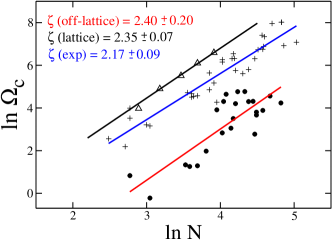
Figure 11: Plot of ln$\Omega_{c}$ as a function of ln$N$. The red line is a fit to the simulation data for the 23 off-lattice Go proteins from which we estimate $\zeta=2.40\pm 0.20$. The black line is a fit to the lattice models with side chains ($N=18,24,32,40$ and 50) with $\zeta=2.35\pm 0.07$. The blue line is a fit to the experimental values of $\Omega_{c}$ for 34 proteins (Table 2) with $\zeta=2.17\pm 0.09$. The larger deviation in $\zeta$ for the minimal models is due to lack of all the interactions that stabilize the NS.

For the thirty four proteins (Table 2) for which we could find thermal denaturation data, we calculated $\Omega_{c}$ using the $\Delta H$, and $T_{F}$ (referred to as the melting temperature $T_{m}$ in the experimental literature).

From the plot of ln$\Omega_{c}$ versus ln$N$ we find that $\zeta=2.17\pm 0.09$. The experimental value of $\zeta$, which also deviates from $\zeta=2$, is in much better agreement with the theoretical prediction. The analysis of experimental data requires care because the compiled results were obtained from a number of different laboratories around the world. Each laboratory uses different methods to analyze the raw experimental data which invariably lead to varying methods to estimate errors in $\Delta H$ and $T_{m}$. To estimate the error bar for $\zeta$ it is important to consider the errors in the computation of $\Omega_{c}$. Using the reported experimental errors in $T_{m}$ and $\Delta H$ we calculated the variance $\delta^{2}\Omega_{c}$ using the standard expression for the error propagation MSLi_PRL04 .

4.3.2 Dependence of folding free energy barrier on number of amino acids $N$

The simultaneous presence of stabilizing (between hydrophobic residues) and destabilizing interactions involving polar and charged residues in polypeptide chain renders the NS only marginally stable Poland_book . The hydrophobic residues enable the formation of compact structures while polar and charged residues, for whom water is a good solvent, are better accommodated by extended conformations. Thus, in the folded state the average energy gain per residue (compared to expanded states) is $-\epsilon_{H}(\approx(1-2)$ kcal/mol) whereas due to chain connectivity and surface area burial the loss in free energy of exposed residues is $\epsilon_{P}\approx\epsilon_{H}$. Because there is a large number of solvent-mediated interactions that stabilize the NS, even when $N$ is small, it follows from the central limit theorem that the barrier height $\beta\Delta G^{\ddagger}$, whose lower bound is the stabilizing free energy should scale as $\Delta G^{\ddagger}\sim k_{B}T\sqrt{N}$ Thirumalai_JPI95 .

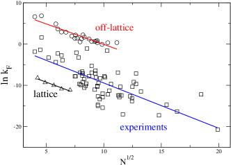
Figure 12: Folding rate of 69 real proteins (squares) is plotted as a function of $N^{1/2}$ (the straight line represent the fit $y=1.54-1.10x$ with the correlation coefficient $R=0.74$). The open circles represent the data obtained for 23 off-lattice Go proteins (see Table 1) (the linear fit $y=9.84-x$ and $R=0.92$). The triangles denote the data obtained for lattice models with side chains ($N=18,24,32,40$ and 50, the linear fit $y=-4.01-1.1x$ and $R=0.98$). For real proteins and off-lattice Go proteins $k_{F}$ is measured in $\mu s^{-1}$, whereas for the lattice models it is measured in MCS^-1 where MCS is Monte Carlo steps.

A different physical picture has been used to argue that $\Delta G^{\ddagger}\sim k_{B}TN^{2/3}$ Finkelstein_FoldDes97 ; Wolynes_PNAS97 . Both the scenarios show that the barrier to folding rates scales sublinearly with $N$.

The dependence of ln$k_{F}$ ($k_{F}=\tau_{F}^{-1}$) on $N$ using experimental data for 69 proteins Naganathan_JACS05 and the simulation results for the 23 proteins is consistent with the predicted behavior that $\Delta G^{\ddagger}=ck_{B}T\sqrt{N}$ with $c\approx 1$ (Fig. 12). The correlation between the experimental results and the theoretical fit is 0.74 which is similar to the previous analysis using a set of 57 proteins MSLi_Polymer04 . It should be noted that the data can also be fit using $\Delta G^{\ddagger}\sim k_{B}TN^{2/3}$. The prefactor $\tau_{F}^{0}$ using the $N^{2/3}$ fit is over an order of magnitude larger than for the $N^{1/2}$ behavior. In the absence of accurate measurements for a larger data set of proteins it is difficult to distinguish between the two power laws for $\Delta G^{\ddagger}$.

Protein	$N$	PDB codea	$\Omega_{c}^{\rm b}$	$\delta\Omega_{c}^{\rm c}$
$\beta$-hairpin	$16$	1PGB	2.29	0.02
$\alpha$-helix	$21$	no code	0.803	0.002
WW domain	$34$	1PIN	3.79	0.02
Villin headpiece	$36$	1VII	3.51	0.01
YAP65	$40$	1K5R	3.63	0.05
E3BD	$45$		7.21	0.05
hbSBD	$52$	1ZWV	51.4	0.2
Protein G	$56$	1PGB	16.98	0.89
SH3 domain ($\alpha$-spectrum)	$57$	1SHG	74.03	1.35
SH3 domain (fyn)	$59$	1SHF	103.95	5.06
IgG-binding domain of streptococcal protein L	$63$	1HZ6	21.18	0.39
Chymotrypsin Inhibitor 2 (CI-2)	$65$	2CI2	33.23	1.66
CspB (Bacillus subtilis)	$67$	1CSP	66.87	2.18
CspA	$69$	1MJC	117.23	13.33
Ubiquitin	$76$	1UBQ	117.8	11.1
Activation domain procarboxypeptidase A2	$80$	1AYE	73.7	3.1
His-containing phosphocarrier protein	$85$	1POH	74.52	4.2
hbLBD	$87$	1K8M	15.8	0.2
Tenascin (short form)	$89$	1TEN	39.11	1.14
Twitchin Ig repeat 27	$89$	1TIT	44.85	0.66
S6	$97$	1RIS	48.69	1.31
FKBP12	$107$	1FKB	95.52	3.85
Ribonuclease A	$124$	1A5P	69.05	2.84

Table 1: List of 23 proteins used in the simulations. (a) The NS for use in the Go model is obtained from the structures deposited in the Protein Data Bank. (b) $\Omega_{c}$ is calculated using equation (21). (c) 2 $\delta\Omega_{c}=|\Omega_{c}-\Omega_{c_{1}}|+|\Omega_{c}-\Omega_{c_{2}}|$, where $\Omega_{c_{1}}$ and $\Omega_{c_{2}}$ are values of the cooperativity measure obtained by retaining only one-half the conformations used to compute $\Omega_{c}$.

Previous studies Klimov_JCP98 have shown that there is a correlation between folding rates and $Z$-score which can be defined as

$$Z_{G}\;=\;\frac{G_{N}-<G_{U}>}{\sigma},$$ (35)

where $G_{N}$ is the free energy of the NS, $<G_{U}>$ is the average free energy of the unfolded states and $\sigma$ is the dispersion in the free energy of the unfolded states. From the fluctuation formula it follows that $\sigma=\sqrt{k_{B}T^{2}C_{p}}$ so that

$$Z_{G}\;=\;\frac{\Delta G}{\sqrt{k_{B}T^{2}C_{p}}}.$$ (36)

Since $\Delta G$ and $C_{p}$ are extensive it follows that $Z_{G}\sim N^{1/2}$. This observation establishes an intrinsic connection between the thermodynamics and kinetics of protein folding that involves formation and rearrangement of non-covalent interactions. In an interesting recent note Naganathan_JACS05 it has been argued that the finding $\Delta G^{\ddagger}\sim k_{B}T\sqrt{N}$ can be interpreted in terms of $n_{\sigma}$ in which $\Delta G$ in Eq. (36) is replaced by $\Delta H$. In either case, there appears to be a thermodynamic rationale for the sublinear scaling of the folding free energy barrier.

Protein	$N$	$\Omega_{c}^{a}$	$\delta\Omega_{c}^{b}$		Protein	$N$	$\Omega_{c}^{a}$	$\delta\Omega_{c}^{b}$
BH8 $\beta$-hairpin Dyer	12	12.9	0.5		SS07d Knapp_JMB96	64	555.2	56.2
HP1 $\beta$-hairpin Xu_JACS03	15	8.9	0.1		CI2 Jackson_Biochemistry91	65	691.2	17.0
MrH3a $\beta$-hairpin Dyer	16	54.1	6.2		CspTm Wassenberg_JMB99	66	558.2	56.3
$\beta$-hairpin Honda_JMB00	16	33.8	7.4		Btk SH3 Knapp_Proteins98	67	316.4	25.9
Trp-cage protein Qui_JACS02	20	24.8	5.1		binary pattern protein Roy_Biochemistry00	74	273.9	30.5
$\alpha$-helix Williams_Biochemistry96	21	23.5	7.9		ADA2h Villegas_Biochemistry95	80	332.0	35.2
villin headpeace Kubelka_JMB03	35	112.2	9.6		hbLBD Naik_ProtSc04	87	903.1	11.1
FBP28 WW domainc Ferguson_PNAS01	37	107.1	8.9		tenascin Fn3 domain Clarke_JMB97	91	842.4	56.6
FBP28 W30A WW domainc Ferguson_PNAS01	37	90.4	8.8		Sa RNase Pace_JMB98	96	1651.1	166.6
WW prototypec Ferguson_PNAS01	38	93.8	8.4		Sa3 RNase Pace_JMB98	97	852.7	86.0
YAP WWc Ferguson_PNAS01	40	96.9	18.5		HPr VanNuland_Biochemistry98	98	975.6	61.9
BBL Ferguson_p	47	128.2	18.0		Sa2 RNase Pace_JMB98	99	1535.0	156.9
PSBD domain Ferguson_p	47	282.8	24.0		barnase Martinez_Biochemistry_94	110	2860.1	286.0
PSBD domain Ferguson_p	50	176.2	13.0		RNase A Arnold_Biochemistry97	125	3038.5	42.6
hbSBD Kouza_BJ05	52	71.8	6.3		RNase B Arnold_Biochemistry97	125	3038.4	87.5
B1 domain of protein G Alexander_Biochemistry92	56	525.7	12.5		lysozyme Hirai_JPC99	129	1014.1	187.3
B2 domain of protein G Alexander_Biochemistry92	56	468.4	20.0		interleukin-1$\beta$ Makhatadze_Biochemistry94	153	1189.6	128.6

Table 2: List of 34 proteins for which $\Omega_{c}$ is calculated using experimental data. The calculated $\Omega_{c}$ values from experiments are significantly larger than those obtained using the Go models (see Table 1). a) $\Omega_{c}$ is computed at $T=T_{F}=T_{m}$ using the experimental values of $\Delta H$ and $T_{m}$. b) The error in $\delta\Omega_{c}$ is computed using the proceedure given in MSLi_PRL04 ; Gutin_PRL96 . c) Data are averaged over two salt conditions at pH 7.0.

4.4 Conclusions

We have reexamined the dependence of the extent of cooperativity as a function of $N$ using lattice models with side chains, off-lattice models and experimental data on thermal denaturation. The finding that $\Omega_{c}\sim N^{\zeta}$ at $T\approx T_{F}$ with $\zeta>2$ provides additional support for the earlier theoretical predictions MSLi_PRL04 . More importantly, the present work also shows that the theoretical value for $\zeta$ is independent of the precise model used which implies that $\zeta$ is universal. It is surprising to find such general characteristics for proteins for which specificity is often an important property. We should note that accurate value of $\zeta$ and $\Omega_{c}$ can only be obtained using more refined models that perhaps include desolvation penalty Kaya_JMB03 ; Cheung_PNAS02

In accord with a number of theoretical predictions Thirumalai_JPI95 ; Finkelstein_FD97 ; Wolynes_PNAS97 ; Gutin_PRL96 ; Li_JPCB02 ; Koga_JMB01 we found that the folding free energy barrier scales only sublinearly with $N$. The relatively small barrier is in accord with the marginal stability of proteins. Since the barriers to global unfolding is relatively small it follows that there must be large conformational fluctuations even when the protein is in the NBA. Indeed, recent experiments show that such dynamical fluctuations that are localized in various regions of a monomeric protein might play an important functional role. These observations suggest that small barriers in proteins and RNA Hyeon_Biochemistry05 might be an evolved characteristics of all natural sequences.

Chapter 5 Folding of the protein hbSBD

5.1 Introduction

Understanding the dynamics and mechanism of protein folding remains one of the most challenging problems in molecular biology Dagget_Trends03 . Single domain $\alpha$ proteins attract much attention of researchers because most of them fold faster than $\beta$ and $\alpha\beta$ proteins Jackson_FD98 ; Kubelka_COSB04 due to relatively simple energy landscapes and one can, therefore, use them to probe main aspects of the funnel theory Bryngelson_Proteins1995 . Recently, the study of this class of proteins becomes even more attractive because the one-state or downhill folding may occur in some small $\alpha$-proteins Munoz_Science02 . The mammalian mitochondrial branched-chain $\alpha$-ketoacid dehydrogenase (BCKD) complex catalyzes the oxidative decarboxylation of branched-chain $\alpha$-ketoacids derived from leucine, isoleucine and valine to give rise to branched-chain acyl-CoAs. In patients with inherited maple syrup urine disease, the activity of the BCKD complex is deficient, which is manifested by often fatal acidosis and mental retardation ccf1 . The BCKD multi-enzyme complex (4,000 KDa in size) is organized about a cubic 24-mer core of dihydrolipoyl transacylase (E2), with multiple copies of hetero-tetrameric decarboxylase (E1), a homodimeric dihydrogenase (E3), a kinase (BCK) and a phosphatase attached through ionic interactions. The E2 chain of the human BCKD complex, similar to other related multi-functional enzymes ccf2 , consists of three domains: The amino-terminal lipoyl-bearing domain (hbLBD, 1-84), the interim E1/E3 subunit-binding domain (hbSBD, 104-152) and the carboxy-terminal inner-core domain. The structures of these domains serve as bases for modeling interactions of the E2 component with other components of $\alpha$-ketoacid dehydrogenase complexes. The structure of hbSBD (Fig. 13a) has been determined by NMR spectroscopy, and the main function of the hbSBD is to attach both E1 and E3 to the E2 core ccf3 . The two-helix structure of this domain is reminiscent of the small protein BBL Ferguson_JMB04 which may be a good candidate for observation of downhill folding Munoz_Science02 ; Munoz_JACS04 . So the study of hbSBD is interesting not only because of the important biological role of the BCKD complex in human metabolism but also for illuminating folding mechanisms.

From the biological point of view, hbSBD could be less stable than hbLBD and one of our goals is, therefore, to check this by the CD experiments. In this paper we study the thermal folding-unfolding transition in the hbSBD by the CD technique in the absence of urea and pH=7.5. Our thermodynamic data do not show evidence for the downhill folding and they are well fitted by the two-state model. We obtained folding temperature $T_{F}=317.8\pm 1.95$ K and the transition enthalpy $\Delta H_{G}=19.67\pm 2.67$ kcal/mol. Comparison of such thermodynamic parameters of hbSBD with those for hbLBD shows that hbSBD is indeed less stable as required by its biological function. However, the value of $\Delta H_{G}$ for hbSBD is still higher than those of two-state $\alpha$-proteins reported in Eaton_COSB04 , which indicates that the folding process in the hbSBD domain is highly cooperative.

Figure 13: (a) Ribbon representation of the structure of hbSBD domain. The helix region H₁ and H₂ include residues Pro12 - Glu20 and Lys39 - Glu47, respectively. (b) Dependence of the mean residue molar ellipticity on the wave length for 18 values of temperatures between 278 and 363 K.

From the theoretical point of view it is very interesting to establish if the two-state foldability of hbSBD can be captured by some model. The all-atom model would be the best choice for a detailed description of the system but the study of hbSBD requires very expensive CPU simulations. Therefore we employed the off-lattice coarse-grained Go-like model Go_ARBB83 ; Clementi_JMB00 which is simple and allows for a thorough characterization of folding properties. In this model amino acids are represented by point particles or beads located at positions of $C_{\alpha}$ atoms. The Go model is defined through the experimentally determined native structure ccf3 , and it captures essential aspects of the important role played by the native structure Clementi_JMB00 ; Takada_PNAS1999 .

It should be noted that the Go model by itself can not be employed to ascertain the two-state behavior of proteins. However, one can use it in conjunction with experiments providing the two-state folding because this model does not always provide the two-state behavior as have been clearly shown in the seminal work of Clementi et al. Clementi_JMB00 . In fact, the Go model correctly captures not only the two-state folding of proteins CI2 and SH3 (more two-state Go folders may be found in Ref. Koga_JMB01 ) but also intermediates of the three-state folder barnase, RNAse H and CheY Clementi_JMB00 . The reason for this is that the simple Go model ignores the energetic frustration but it still takes the topological frustration into account. Therefore, it can capture intermediates that occur due to topological constraints but not those emerging from the frustration of the contact interactions. With the help of Langevin dynamics simulations and the histogram method Ferrenberg_PRL89 we have shown that, in agreement with our CD data, hbSBD is a two-state folder with a well-defined TS in the free energy landscape. The two helix regions were found to be highly structured in the TS. The two-state behavior of hbSBD is also supported by our kinetics study showing that the folding kinetics follows the single exponential scenario. The two-state folding obtained in our simulations suggests that for hbSBD the topological frustration is more important than the energetic factor.

The dimensionless quantity, $\Omega_{c}$ Klimov_FD98 , which characterizes the structural cooperativity of the thermal denaturation transition was computed and the reasonable agreement between the CD experiments and Go simulations was obtained. Incorporation of side chains may give a better agreement Klimov_FD98 ; Li_Physica05 but this problem is beyond the scope of the thesis.

The material presented in this chapter is based on our work Kouza_BJ05 .

5.2 Materials and Methods

5.2.1 Sample Preparation

hbSBD protein was purified from the BL21(DE3) strain of E. coli containing a plasmid that carried the gene of hbLBD(1-84), a TEV cleavage site in the linker region, and hbSBD (104-152), generously provided to us by Dr. D.T. Chuang of the Southwestern Medical Center, University of Texas. There is an extra glycine in front of Glu104 which is left over after TEV cleavage, and extra leucine, glutamic acid at the C-terminus before six histidine residues. The protein was purified by Ni-NTA affinity chromatography, and the purity of the protein was found to be better than 95%, based on the Coomassie blue-stained gel. The complete sequence of $N=52$ residues for hbSBD is
(G)EIKGRKTLATPAVRRLAMENNIKLSEVVGSGKDGRILKEDILNYLEKQT(L)(E).

5.2.2 Circular Dichroism

CD measurements were carried out in Aviv CD spectrometer model 202 with temperature and stir control units at different temperature taken from 260nm to 195nm. All experiments were carried at 1 nm bandwidth in 1.0 cm quartz square cuvette thermostated to $\pm 0.1^{o}$C. Protein concentration ($\sim$ 50 uM) was determined by UV absorbance at 280nm using $\epsilon_{280nm}$=1280 M^-1cm^-1 with 50mM phosphate buffer at pH7.5. Temperature control was achieved using a circulating water bath system, and the equilibrium time was three minutes for each temperature point. The data was collected at each 2K increment in temperature. The study was performed at heating rate of 10^oC/min and equilibration time of 3 minutes. The volume changes as a result of thermal expansion as well as evaporation of water were neglected.

5.2.3 Fitting Procedure

Suppose the thermal denaturation is a two-state transition, we can write the ellipticity as

$$\theta\;\,=\;\,\theta_{D}+(\theta_{N}-\theta_{D})f_{N}\,,$$ (37)

where $\theta_{D}$ and $\theta_{N}$ are values for the denaturated and folded states. The fraction of the folded conformation $f_{N}$ is expressed as Privalov_APC79

$$f_{N}\;\, = \;\,\frac{1}{1+\exp(-\Delta G_{T}/T)}\,,$$

$$\Delta G_{T}\;\, = \;\,\Delta H_{T}-T\Delta S_{T}\;=\;\Delta H_{G}\left(1-\frac{T}{T_{G}}\right)$$ (38)

$$+ \Delta C_{p}\left[(T-T_{G})-T\ln\frac{T}{T_{G}}\right]\,.$$

Here $\Delta H_{G}$ and $\Delta C_{p}$ are jumps of the enthalpy and heat capacity at the mid-point temperature $T_{G}$ (also known as melting or folding temperature) of thermal transition, respectively. Some other thermodynamic characterization of stability such as the temperature of maximum stability ($T_{S}$), the temperature with zero enthalpy ($T_{H}$), and the conformational stability ($\Delta G_{S}$) at $T_{S}$ can be computed from results of regression analysis Becktel_Biopolymers87

$$\ln\frac{T_{G}}{T_{S}}\; = \;\frac{\Delta H_{G}}{T_{G}\Delta C_{p}},$$ (39)

$$T_{H}\; = \;T_{G}-\frac{\Delta H_{G}}{\Delta C_{p}},$$ (40)

$$\Delta G_{S}\; = \;\Delta C_{p}(T_{S}-T_{H}).$$ (41)

Using Eqs. (37) - (41) we can obtain all thermodynamic parameters from CD data.

It should be noted that the fitting of Eq. (38) with $\Delta C_{p}>0$ allows for an additional cold denaturation Privalov_CRBMB90 at temperatures much lower than the room temperature . The temperature of such a transition, $T_{G}^{\prime}$, may be obtained by the same fitting procedure with an additional constraint of $\Delta H_{G}<0$. Since the cold denaturation transition is not seen in Go models, to compare the simulation results to the experimental ones we also use the approximation in which $\Delta C_{p}=0$.

5.2.4 Simulation

We use coarse-grained continuum representation for hbSBD protein, in which only the positions of 52 C_α-carbons are retained. We adopt the off-lattice version of the Go model Go_ARBB83 where the interaction between residues forming native contacts is assumed to be attractive and the non-native interactions - repulsive (Eq. 5).

The nativeness of any configuration is measured by the number of native contacts $Q$. We define that the $i$th and $j$th residues are in the native contact if $r_{0ij}$ is smaller than a cutoff distance $d_{c}$ taken to be $d_{c}=7.5$ Å, where $r_{0ij}$ is the distance between the $i$th and $j$th residues in the native conformation. Using this definition and the native conformation of Ref. ccf3, , we found that the total number of native contacts $Q_{total}=62$. To study the probability of being in the NS we use the following overlap function as in Eq. (22).

The overlap function $\chi$, which is one if the conformation of the polypeptide chain coincides with the native structure and zero for unfolded conformations, can serve as an order parameter for the folding-unfolding transition. The probability of being in the NS, $f_{N}$, which can be measured by the CD and other experimental techniques, is defined as $f_{N}=<\chi>$, where $<...>$ stands for a thermal average.

The dynamics of the system is obtained by integrating the following Langevin equation Allen_book (Eq. 15). The Verlet algorithm Swope_JCP82 was employed. It should be noted that the folding thermodynamics does not depend on the environment viscosity (or on $\zeta$) but the folding kinetics depends on it Klimov_PRL97 . We chose the dimensionless parameter $\tilde{\zeta}=(\frac{a^{2}}{m\epsilon_{H}})^{1/2}\zeta=8$, where $m$ is the mass of a bead and $a$ is the bond length between successive beads. One can show that this value of $\tilde{\zeta}$ belongs to the interval of the viscosity where the folding kinetics is fast. We have tried other values of $\tilde{\zeta}$ but the results remain unchanged qualitatively. All thermodynamic quantities are obtained by the histogram method Ferrenberg_PRL89 .

5.3 Results

5.3.1 CD Experiments

The structure of hbSBD is shown in Figure 13a. Its conformational stability is investigated in present study by analyzing the unfolding transition induced by temperature as monitored by CD, similar to that described previously Naik_FEBS02 ; Naik_ProtSc04 . The reversibility of thermal denaturation was ascertained by monitoring the return of the CD signal upon cooling from 95^oC to 22 ^oC; immediately after the conclusion of the thermal transition. The transition was found to be more than 80% reversible. Loss in reversibility to greater extent was observed on prolonged exposure of the sample to higher temperatures. This loss of reversibility is presumably due to irreversible aggregation or decomposition. Figure 13b shows the wavelength dependence of mean residue molar ellipticity of hbSBD at various temperatures between 278K and 363K. In a separate study, the thermal unfolding transition as monitored by ellipticity at 228 nm was found to be independent of hbSBD concentration in the range of 2 uM to 10 uM. It was also found to be unaffected by change in heating rate between 2^oC/min to 20^oC/min. These observations suggest absence of stable intermediates in heat induced denaturation of hbSBD. A valley at around 220 nm, characteristics of the helical secondary structure is evident for hbSBD.

Figure 14a shows the temperature dependence of the population of the native conformation, $f_{N}$, for wave lengths $\lambda=208,212$ and 222 nm. We first try to fit these data to Eq. (38) with $\Delta C_{p}\neq 0$. The fitting procedure gives slightly different values for the folding (or melting) temperature and the enthalpy jump for three sets of parameters. Averaging over three values, we obtain $T_{G}=317.8\pm 1.95$ K and $\Delta H_{G}=19.67\pm 2.67$ kcal/mol. Other thermodynamic quantities are shown on the first row of Table 3. The similar fit but with $\Delta C_{p}=0$ gives the thermodynamic parameters shown on the second row of this table. Since the experimental data are nicely fitted to the two-state model we expect that the downhill scenario does not applied to the hbSBD domain.

Figure 14: (a) Temperature dependence of the fraction of folded conformations $f_{N}$, obtained from the ellipticity $\theta$ by Eq. (38), for wave lengths $\lambda$ = 208 (blue circles), 212 (red squares) and 222 nm (green diamonds). The solid lines corresponds to the two state fit given by Eq. (38) with $\Delta C_{p}\neq 0$. We obtained $T_{G}=T_{F}=317.8\pm 1.9$ K, $\Delta H_{G}=19.67\pm 2.67$ kcal/mol and $\Delta C_{p}=0.387\pm 0.054$. (b) The dependence of $f_{N}$ for various sets of parameters. The blue and red curves correspond to the thermodynamic parameters presented on the first and the second rows of Table 3, respectively. Open circles refer to simulation results for the Go model. The solid black curve is the two-state fit ($\Delta C_{p}=0$) which gives $\Delta H_{G}=11.46$ kcal/mol and $T_{F}=317.9$. (c) The upper part refers to the temperature dependence of $df_{N}/dT$ obtained by the simulations (red) and the CD experiments (blue). The experimental curve is plotted using two-state parameters with $\Delta C_{p}=0$ (see, the second row on Table 3). The temperature dependence of the heat capacity $C_{V}(T)$ is presented in the lower part. The dotted lines illustrate the base line substraction. The results are averaged over 20 samples.

For the experimentally studied temperature interval two types of the two-state fit (38) with $\Delta C_{p}=0$ and $\Delta C_{p}\neq 0$ give almost the same values for $T_{G}$, $\Delta H_{G}$ and $\Delta S_{G}$. However, pronounced different behaviors of the population of the native basin, $f_{N}$, occur when we interpolate results to the low temperature region (Fig. 14b). For the $\Delta C_{p}=0$ case, $f_{N}$ approaches the unity as $T\rightarrow 0$ but it goes down for $\Delta C_{p}\neq 0$. This means that the $\Delta C_{p}\neq 0$ fit is valid if the second cold denaturation transition may occur at $T_{G}$’. This phenomenon was observed in single domains as well as in multi-domain globular proteins Privalov_CRBMB90 . We predict that the cold denaturation of hbSBD may take place at $T_{G}^{\prime}\approx 212$ K which is lower than $T_{G}^{\prime}\approx 249.8$ K for hbLBD shown on the 4th row of Table 3. It would be of great interest to carry out the cold denaturation experiments in cryo-solvent to elucidate this issue.

To compare the stability of the hbSBD domain with the hbLBD domain which has been studied in detail previously Naik_ProtSc04 we also present the thermodynamic data of the latter on Table 3. Clearly, hbSBD is less stable than hbLBD by its smaller $\Delta G_{S}$ and lower $T_{G}$ values. This is consistent with their respective backbone dynamics as revealed by ¹⁵N-T₁, ¹⁵N-T₂, and ¹⁵N-¹H NOE studies of these two domains using uniformly ¹⁵N-labeled protein samples (Chang and Huang, unpublished results). Biologically, hbSBD must bind to either E1 or E3 at different stages of the catalytic cycle, thus it needs to be flexible to adapt to local environments of the active sites of E1 and E3. On the other hand, the function of hbLBD is to permit its Lys44 residue to channel acetyl group between donor and acceptor molecules and only the Lys44 residue needs to be flexible Chang_JBC02 . In addition, the NMR observation for the longer fragment (comprising residues 1-168 of the E2 component) also showed that the hbLBD region would remain structured after several months while the hbSBD domain could de-grate in a shorter time.

		$\Delta{H}_{G}$	$\Delta{C_{p}}$	$\Delta{S_{G}}$			$\Delta{G_{S}}$
Domain	$T_{G}(K)$	kcal/mol/K)	(kcal/mol/K)	(cal/mol/K)	$T_{S}(K)$	$T_{H}(K)$	(kcal/mol)	$T^{\prime}_{G}(K)$
SBD(exp)	$317.8\pm 1.9$	$19.67\pm 2.67$	$0.387\pm 0.054$	$61.64\pm 7.36$	$270.9\pm 2.0$	$267.0\pm 2.1$	$1.4\pm 0.1$	$212\pm 2.5$
SBD(exp)	$317.9\pm 2.2$	$20.02\pm 3.11$	$0.0$	$62.96\pm 9.92$	$-$	$-$	$-$	-
SBD(sim)	$317.9\pm 7.95$	$11.46\pm 0.29$	$0.0$	$36.05\pm 1.85$	$-$	$-$	$-$	-
LBD(exp)	$344.0\pm 0.2$	$78.96\pm 1.28$	$1.51\pm 0.04$	$229.5\pm 3.7$	$295.7\pm 3.7$	$291.9\pm 1.3$	$5.7\pm 0.2$	$249.8\pm 1.1$

Table 3: Thermodynamic parameters obtained from the CD experiments and simulations for hbSBD domain. The results shown on the first and fourth rows were obtained by fitting experimental data to the two-state equation (38) with $\Delta C_{p}\neq 0$. The second and third rows corresponding to the fit with $\Delta C_{p}=0$. The results for hbLBD are taken from Ref. Naik_ProtSc04 for comparison.

5.3.2 Folding Thermodynamics from simulations

In order to calculate the thermodynamics quantities we have collected histograms for the energy and native contacts at six values of temperature: $T=0.4,0.5,0.6,0.7,0.8$ and 1.0 $\epsilon_{H}/k_{B}$. For sampling, at each temperature 30 trajectories of $16\times 10^{7}$ time steps have been generated with initial $4\times 10^{7}$ steps discarded for thermalization. The reweighting histogram method Ferrenberg_PRL89 was used to obtain the thermodynamics parameters at all temperatures.

Figure 14b (open circles) shows the temperature dependence of population of the NS, defined as the renormalized number of native contacts for the Go model. Since there is no cold denaturation for this model, to obtain the thermodynamic parameters we fit $f_{N}$ to the two-state model (Eq. 38) with $\Delta C_{p}=0$.

The fit (black curve) works pretty well around the transition temperature but it gets worse at high $T$ due to slow decay of $f_{N}$ which is characteristic for almost all of theoretical models. In fitting we have chosen the hydrogen bond energy $\epsilon_{H}=0.91$ kcal/mol in Hamiltonian (5) so that $T_{G}=0.7\epsilon_{H}/k_{B}$ coincides with the experimental value 317.8 K. From the fit we obtain $\Delta H_{G}=11.46$ kcal/mol which is smaller than the experimental value indicating that the Go model is less stable compared to the real hbSBD.

Figure 14c shows the temperature dependence of derivative of the fraction of native contacts with respect to temperature $df_{N}/dT$ and the specific heat $C_{v}$ obtained from the Go simulations. The collapse temperature $T_{\theta}$, defined as the temperature at which $C_{v}$ is maximal, almost coincides with the folding temperature $T_{F}$ (at $T_{F}$ the structural susceptibility has maximum). According to Klimov and Thirumalai Klimov_PRL96 , the dimensionless parameter $\sigma=\frac{|T_{\theta}-T_{F}|}{T_{F}}$ may serve as an indicator for foldablity of proteins. Namely, sequences with $\sigma\leq 0.1$ fold much faster that those which have the same number of residues but with $\sigma$ exceeding 0.5. From this perspective, having $\sigma\approx 0$ hbSBD is supposed to be a good folder in silico. However, one has to be cautious about this conclusion because the pronounced correlation between folding times $\tau_{F}$ and the equilibrium parameter $\sigma$, observed for simple on- and off-lattice models Klimov_PRL96 ; Veitshans_FD97 may be not valid for proteins in laboratory Gillepse_ARB04 . In our opinion, since the data collected from theoretical and experimental studies are limited, further studies are required to clarify the relationship between $\tau_{F}$ and $\sigma$.

Using experimental values for $T_{G}$ (as $T_{F}$) and $\Delta H_{G}$ and the two-state model with $\Delta C_{p}=0$ (see Table 3) we can obtain the temperature dependence of the population of NS $f_{N}$ and, therefore, $df_{N}/dT$ for hbSBD (Fig. 14c). Clearly, the folding-unfolding transition in vitro is sharper than in the Go modeling. One of possible reasons is that our Go model ignores the side chain which can enhance the cooperativity of the denaturation transition Klimov_FD98 .

The sharpness of the fold-unfolded transition might be characterized quantitatively via the cooperativity index $\Omega_{c}$ (Eq. 21). From Fig. 14c, we obtain $\Omega_{c}=51.6$ and 71.3 for the Go model and CD experiments, respectively. Given the simplicity of the Go model used here the agreement in $\Omega_{c}$ should be considered reasonable. We can also estimate $\Omega_{c}$ from the scaling law suggested in Ref. MSLi_PRL04, , $\Omega_{c}=0.0057\times N^{\mu}$, where exponent $\mu$ is universal and expressed via the random walk susceptibility exponent $\gamma$ as $\mu=1+\gamma\approx 2.22(\gamma\approx 1.22$). Then we get $\Omega_{c}\approx 36.7$ which is lower than the experimental as well as simulation result. This means that hbSBD in vitro is, on average, more cooperative than other two-state folders.

Another measure for the cooperativity is $\kappa_{2}$ which is defined as Kaya_PRL00 $\kappa_{2}=\Delta H_{vh}/\Delta H_{cal}$, where $\Delta H_{vh}\;=\;2T_{max}\sqrt{k_{B}C_{V}(T_{max})}$ and $\Delta H_{cal}\;=\;\int_{0}^{\infty}C_{V}(T)dT$, are the van’t Hoff and the calorimetric enthalpy, respectively, $C_{V}(T)$ is the specific heat. Without the baseline substraction in $C_{V}(T)$ Chan_ME04 , for the Go model of hbSBD we obtained $\kappa_{2}\approx 0.25$. Applying the baseline substraction as shown in the lower part of Fig. 14c we got $\kappa_{2}\approx 0.5$ which is still much lower than $\kappa_{2}\approx 1$ for a truly all-or-none transition. Since $\kappa_{2}$ is an extensive parameter, its low value is due to the shortcomings of the off-lattice Go models but not due to the finite size effects. More rigid lattice models give better results for the calorimetric cooperativity Li_Physica05 . Thus, for the hbSBD domain the Go model gives the better agreement with our CD experiments for the structural cooperativity $\Omega_{c}$ than for the calorimetric measure $\kappa_{2}$.

5.3.3 Free Energy Profile

To get more evidence that hbSBD is a two-state folder we study the free energy profile using some quantity as a reaction coordinate. The precise reaction coordinate for a multi-dimensional process such as protein folding is difficult to ascertain. However, Onuchic and coworkers Nymeyer_PNAS98 have argued that, for minimally frustrated systems such as Go models, the number of native contact $Q$ may be appropriate. Fig. 15a shows the dependence of free energy on $Q$ for $T=T_{F}$. Since there is only one local maximum corresponding to the transition state (TS), hbSBD is a two-state folder. This is not unexpectable for hbSBD which contains only helices. The fact that the simple Go model correctly captures the two-state behavior as was observed in the CD experiments, suggests that the energetic frustration ignored in this model plays a minor role compared to the topological frustration Clementi_JMB00 .

Figure 15: (a) The dependence of free energy on the number of native contacts $Q$ at $T=T_{F}$. The typical structures of the DS , TS and folded state are also drawn. The helix regions H₁ (green) and H₂ (orange) of the TS structure involve residues 13 - 19 and 39 - 48, respectively. For the folded state structure H₂ is the same as for the TS structure but H₁ has two residues more (13 - 21). (b) Distributions of RMSD for three ensembles shown in (a). The average values of RMSD are equal to 9.8, 4.9 and 3.2 Å  for the DS, TS and folded state, respectively.

We have sorted out structures of the DS , TS and the folded state at $T=T_{F}$ generating $10^{4}$ conformations in equilibrium. The distributions of the RMSD, $P_{\rm RMSD}$, of these states are plotted in Fig. 15b. As expected, $P_{\rm RMSD}$ for the DS spreads out more than that for the TS and folded state. According to the free energy profile in Fig. 15a, the TS conformations have 26 - 40 native contacts. We have found that the size (number of folded residues) Bai_ProtSc04 of the TS is equal to 32. Comparing this size with the total number of residues ($N=52$) we see that the fraction of folded residues in the TS is higher than the typical value for real two-state proteins Bai_ProtSc04 . This is probably an artifact of Go models Kouza_BJ05 . The TS conformations are relatively compact having the ratio $<R_{g}^{TS}>/R_{g}^{NS}\approx 1.14$, where $<R_{g}^{TS}>$ is the average radius of gyration of the TS ensemble and $R_{g}^{NS}$ is the radius of gyration of the native conformation shown in Fig. 13a. Since the RMSD, calculated only for two helices, is about 0.8 Åthe structures of two helices in the TS are not distorted much. It is also evident from the typical structure of the TS shown in Fig. 15b where the helix regions H₁ and H₂ involve residues 13 - 19 and 39 - 48, respectively (a residue is considered to be in the helix state if its dihedral angle is about 60^o). Note that H₁ has two residues less compared to H₁ in the native conformation (see the caption to Fig. 13a) but H₂ has even one bead more than its NS counterpart. Overall, the averaged RMSD of the TS conformations from the native conformation (Fig. 13a) is about 4.9 Å  indicating that the TS is not close to the native one. As seen from Figs. 15a and 13a, the main difference comes from the tail parts. The most probable conformations (corresponding to maximum of $P_{\rm RMSD}$ in Fig. 15b of the folded state have RMSD about 2.5 Å. This value is reasonable from the point of view of the experimental structure resolution.

5.3.4 Folding Kinetics

The two-state foldability, obtained from the thermodynamics simulations may be also probed by studying the folding kinetics. For this purpose we monitored the time dependence of the fraction of unfolded trajectories $P_{u}(t)$ defined as follows Klimov_COSB99

$$P_{u}(t)\,=\,1-\int_{0}^{t}P^{\textstyle{N}}_{fp}(s)ds,$$ (42)

where $P^{\textstyle{N}}_{fp}$ is the distribution of first passage folding times

$$P^{\textstyle{N}}_{fp}\,=\,\frac{1}{M}\sum_{i=1}^{M}\delta(s-\tau_{f,1i}).$$ (43)

Here $\tau_{f,1i}$ is time for the $i$th trajectory to reach the NS for the first time, $M$ is the total number of trajectories used in simulations. A trajectory is said to be folded if all of native contacts form. As seen from Eqs. 42 and 43, $P_{u}(t)$ is the fraction of trajectories which do not reach the NS at time $t$. In the two-state scenario the folding becomes triggered after overcoming only one free energy barrier between the TS and the denaturated one. Therefore, $P_{u}(t)$ should be a single exponential, i.e. $P_{u}(t)\sim\exp(-t/\tau_{F})$ (a multi-exponential behavior occurs in the case when the folding proceeds via intermediates) Klimov_COSB99 .

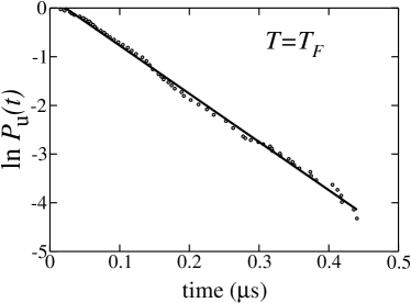
Figure 16: The semi-logarithmic plot of the time dependence of the fraction of unfolded trajectories at $T=T_{F}$. The distribution $P_{u}(t)$ was obtained from first passage times of 400 trajectories, which start from random conformations. The straight line corresponds to the fit ln $P_{\rm u}(t)=-t/\tau_{F}$, where $\tau_{F}=0.1\mu$s.

Since the function $P_{u}(t)$ can be measured directly by a number of experimental techniques Greene_Methods04 ; Dyson_ME2005 , the single exponential kinetics of two-state folders is supported by a large body of experimental work (see, i.e. Ref. Naik_FEBS02 and references there). Fig. 16 shows the semi-logarithmic plot for $P_{u}(t)$ at $T=T_{F}$ for the Go model. Since the single exponential fit works pretty well, one can expect that intermediates do not occur on the folding pathways. Thus, together with the thermodynamics data our kinetic study supports the two-state behavior of the hbSBD domain as observed on the CD experiments.

From the linear fit in Fig. 16 we obtain the folding time $\tau_{F}\approx 0.1\mu$s. This value is consistent with the estimate of the folding time defined as the average value of the first passage times. If we use the empirical formula for the folding time $\tau_{F}=\tau_{F}^{0}\exp(1.1N^{1/2})$, where prefactor $\tau_{F}^{0}=0.4\mu$s and $N$ is a number of amino acids MSLi_Polymer04 then $\tau_{F}=1.1\times 10^{3}\mu$s for $N=52$. This value is about four orders of magnitude larger than that obtained from the Go model. Thus the Go model can capture the two-state feature of the denaturation transition for hbSBD domain but not folding times.

5.4 Discussion

We have used CD technique and the Langevin dynamics to study the mechanism of folding of hbSBD. Our results suggest that this domain is a two-state folder. The CD experiments reveal that the hbSBD domain is less stable than the hbLBD domain in the same BCKD complex, but it is more stable and cooperative compared to other fast folding $\alpha$ proteins.

Both the thermodynamics and kinetics results, obtained from the Langevin dynamics simulations, show that the simple Go model correctly captures the two-state feature of folding. It should be noted that the two-state behavior is not the natural consequence of the Go modeling because it allows for fishing folding intermediates caused by the topological frustration. From this standpoint it may be used to decipher the foldability of model proteins for which the topological frustration dominates. The reasonable agreement between the results obtained by the Go modeling and our CD experiments, suggests that the NS topology of hbSBD is more important than the energetic factor.

The theoretical model gives the reasonable agreement with the CD experimental data for the structural cooperativity $\Omega_{c}$. However, the calorimetric cooperativity criterion $\kappa_{2}\approx 1$ for two-state folders is hard to fulfill within the Go model. From the $\Delta C_{p}\neq 0$ fitting procedure we predict that the cold denaturation of hbSBD may occur at $T\approx 212$ K and it would be very interesting to verify this prediction experimentally. We are using the package SMMP Eisenmenger_CPC01 and a parallel algorithm Hayryan_JCC01 to perform all-atom simulation of hbSBD to check the relevant results.

Chapter 6 Force-Temperature phase diagram of single and three domain ubiquitin. New force replica exchange method

6.1 Introduction

Protein Ub continues to attract the attention of researchers because there exist many processes in living systems where it plays the vital role. Usually, Ub presents in the form of a polyubiquitin chain that is conjugated to other proteins. Different Ub linkages lead to different biological functions. In case of Lys48-C and N-C linkages polyubiquitin chain serves as a signal for degradation proteins Thrower_EMBO2000 ; Kirisako_EMBO2006 , whereas in the Lys63-C case it plays completely different functions, including DNA repair, polysome stability and endocytosis Hofmann_Cell1999 ; Spence_Cell2000 ; Galan_EMBO1997 .

When one studies thermodynamics of a large system like multi-domain Ub the problem of slow dynamics occurs, due to the rough FEL. This problem might be remedied using the standard RE method in the temperature space in the absence of external force Hukushima_JPSC96 ; Sugita_ChemPhysLett99 ; Phuong_Proteins05 as well as in the presence of it Li_JPCB06 . However, if one wants to construct the force-temperature phase diagram, then this approach becomes inconvenient because one has to collect data at different values of forces. Moreover, the external force increases unfolding barriers and a system may get trapped in some local minima. In order to have better sampling for a system subject to external force we propose a new RE method Kouza_JCP08 in which the exchange is carried not in the temperature space but in the force space, i.e. the exchange between different force values. This procedure would help the system to escape from local minima efficiently.

In this chapter we address two topics. First, we develop a new version of the RE method to study thermodynamics of a large system under the force. The basic idea is that for a given temperature we perform simulation at different values of force and the exchange between them is carried out according to the Metropolis rule. This new approach has been employed to obtain the force-temperature phase diagram of the three-domain Ub, which will be referred to as trimer . Within our choice of force replicas it speeds up computation about four times compared to the conventional simulation. Second, we construct the temperature-force $T-f$ phase diagram of Ub and its trimer which allows us to to determine the equilibrium critical force $f_{c}$ separating the folded and unfolded regions.

This chapter is based on Ref. Kouza_JCP08 .

6.2 Model

Figure 17 shows native conformations for single Ub and trimer. Native conformation of Ub is taken form the PDB (1UBQ) and with the choice of cutoff distance $d_{c}=6.5\AA$ it has 99 native contacts. NS of three-domain Ub. is not available yet and we have to construct it for Go modeling. To make it we translate one unit by the distance $a=3.82\AA$ and slightly rotate it, then translate and rotate one more to have nine interdomain contacts (about 10% of the intra-domain contacts). There are 18 inter- and 297 intradomain native contacts.

Figure 17: (a) NS conformation of Ub taken from the PDB (PDB ID: 1ubq). There are five $\beta$-strands: S1 (2-6), S2 (12-16), S3 (41-45), S4 (48-49) and S5 (65-71), and one helix A (23-34). (b) Structures B, C, D and E consist of pairs of strands (S1,S2), (S1,S5), (S3,S5) and (S3,S4), respectively. In the text we also refer to helix A as the structure A. (c) The native conformation of trimer was designed as described in section 6.2. There are 18 inter- and 297 intra-domain native contacts

We use coarse-grained continuum representation for Ub and trimer in which only the positions of $C_{\alpha}$-carbons are retained. The energy of Go-type model Clementi_JMB00 is described by Eq. (5). In order to obtain the $T-f$ phase diagram, we use the fraction of native contacts or the overlap function as in Eq. (22). The $T-f$ phase diagram ( a plot of $1-f_{N}$ as a function of $f$ and $T$) and thermodynamic quantities were obtained by the multiple histogram method Ferrenberg_PRL89 extended to the case when the external force is applied to the termini Klimov_PNAS99 ; Klimov_JPCB01 . In this case the reweighting is carried out not only for temperature but also for force. We collected data for six values of $T$ at $f=0$ and for five values of $f$ at a fixed value of $T$. The duration of MD runs for each trajectory was chosen to be long enough to get the system fully equilibrating (9$\times 10^{5}\tau_{L}$ from which 1.5$\times 10^{5}\tau_{L}$ were spent on equilibration). For a given value of $T$ and $f$ we have generated 40 independent trajectories for thermal averaging.

6.3 Force-Temperature diagram for single ubiquitin

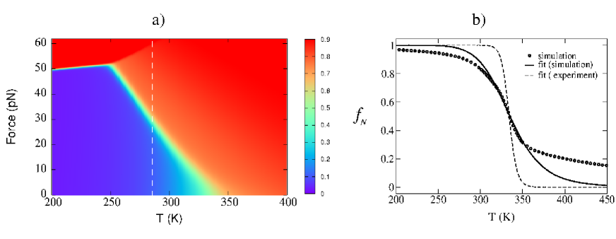
Figure 18: (a) The $T-f$ phase diagram obtained by the extended histogram method. The force is applied to termini N and C. The color code for $1-<\chi(T,f)>$ is given on the right. The blue color corresponds to the state in the NBA, while the red color indicates the unfolded states. The vertical dashed line refers to $T=0.85T_{F}\approx 285$ K at which most of simulations have been performed. (b) The temperature dependence of $f_{N}$ (open circles) defined as the renormalized number of native contacts. The solid line refers to the two-state fit to the simulation data. The dashed line represents the experimental two-state curve with $\Delta H_{\rm m}$ = 48.96 kcal/mol and $T_{m}=332.5$K Thomas_PNAS01 .

The $T-f$ phase diagram, obtained by the extended histogram method, is shown in Fig. 18a. The folding-unfolding transition, defined by the yellow region, is sharp in the low temperature region but it becomes less cooperative (the fuzzy transition region is wider) as $T$ increases. The weak reentrancy (the critical force slightly increases with $T$) occurs at low temperatures. This seemingly strange phenomenon occurs as a result of competition between the energy gain and the entropy loss upon stretching. The similar cold unzipping transition was also observed in a number of models for heteropolymers Shakhnovich_PRE02 and proteins Klimov_PNAS99 including the C_α-Go model for I27 (MS Li, unpublished results). As follows from the phase diagram, at $T=285$ K the critical force $f_{c}\approx 30$ pN which is close to $f_{c}\approx 25$ pN, estimated from the experimental pulling data. To estimate $f_{c}$ from experimental pulling data we use $f_{max}\approx f_{c}{\rm ln}(v/v_{min})$ Evans_BJ97 (see also Eq. 27), where $f_{max}$ is the maximal force needed to unfold a protein at the pulling speed $v$. From the raw data in Fig. 3b of Ref. Carrion-Vazquez_NSB03 we obtain $f_{c}\approx$ 25 pN. Given the simplicity of the model this agreement can be considered satisfactory and it validates the use of the Go model.

Figure 18b shows the temperature dependence of population of the NS. Fitting to the standard two-state curve $f_{N}=\frac{1}{1+\exp[-\Delta H_{m}(1-\frac{T}{T_{m}})/k_{B}T]}$, one can see that it works pretty well (solid curve) around the transition temperature but it gets worse at high $T$ due to slow decay of $f_{N}$. Such a behavior is characteristic for almost all of theoretical models Kouza_BJ05 including the all-atom ones Phuong_Proteins05 . In fitting we have chosen the hydrogen bond energy $\epsilon_{H}=0.98$ kcal/mol in Hamiltonian (5) so that $T_{F}=T_{m}=0.675\epsilon_{H}/k_{B}$ coincides with the experimental value 332.5 K Thomas_PNAS01 . From the fit we obtain $\Delta H_{\rm m}=11.4$ kcal/mol which is smaller than the experimental value 48.96 kcal/mol indicating that the Go model is, as expected, less stable compared to the real Ub. Taking into account non-native contacts and more realistic interactions between side chain atoms is expected to increase the stability of the system.

The cooperativity of the denaturation transition may be characterized by the cooperativity index, $\Omega_{c}$ given by Eq. (21). From simulation data for $f_{N}$ presented

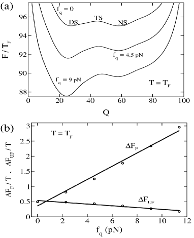
Figure 19: (a) The dependence of the free energy on $Q$ for selected values of $f$ at $T=T_{F}$.(b) The dependence of folding and unfolding barriers, obtained from the free energy profiles, on $f$. The linear fits $y=0.36+0.218x$ and $y=0.54-0.029x$ correspond to $\Delta F_{f}$ and $\Delta F_{u}$, respectively. From these fits we obtain $x_{f}\approx$ 10 nm and $x_{u}\approx$ 0.13 nm.

in Fig. 18b, we have $\Omega_{c}\approx 57$ which is considerably lower than the experimental value $\Omega_{c}\approx 384$ obtained with the help of $\Delta H_{\rm m}$ = 48.96 kcal/mol and $T_{m}=332.5$K Thomas_PNAS01 . The underestimation of $\Omega_{c}$ in our simulations is not only a shortcoming of the off-lattice Go model Kouza_JPCA06 but also a common problem of much more sophisticated force fields in all-atom models Phuong_Proteins05 .

Another measure of the cooperativity is the ratio between the van’t Hoff and the calorimetric enthalpy, $\kappa_{2}$ Kaya_PRL00 . For the Go Ub we obtained $\kappa_{2}\approx 0.19$. Applying the base line subtraction Chan_ME04 gives $\kappa_{2}\approx 0.42$ which is still much below $\kappa_{2}\approx 1$ for the truly one-or-none transition. Since $\kappa_{2}$ is an extensive parameter, its low value is due to the shortcomings of the off-lattice Go models but not due to the finite size effects. More rigid lattice models give better results for the calorimetric cooperativity $\kappa_{2}$ Li_Physica05 .

Figure 19a shows the free energy as a function of $Q$ for several values of force at $T=T_{F}$. Since there are only two minima, our results support the two-state picture of Ub Schlierf_PNAS04 ; Chung_PNAS05 . As expected, the external force increases the folding barrier, $\Delta F_{F}$ ($\Delta F_{F}=F_{TS}-F_{DS}$) and it lowers the unfolding barrier, $\Delta F_{u}$ ($\Delta F_{u}=F_{TS}-F_{NS}$). From the linear fits in Fig. 19b we obtain $x_{f}=\Delta F_{f}/f\approx 1$ nm, and $x_{u}=\Delta F_{u}/f\approx 0.13$ nm. Note that $x_{f}$ is very close to $x_{f}\approx$ 0.96 nm obtained from refolding times at a bit lower temperature $T=285$ K (see Fig. 30 below). However, $x_{u}$ is lower than the experimental value 0.24 nm Carrion-Vazquez_NSB03 . This difference may be caused by either sensitivity of $x_{u}$ to the temperature or the determination of $x_{u}$ from the approximate FEL as a function of a single coordinate $Q$ is not sufficiently accurate. In Chapter 8, we will show that a more accurate estimate of $x_{u}$ may be obtained from the dependence of unfolding times on the external force (Eq. 24).

We have also studied the FEL using $\Delta R$ as a reaction coordinate. The dependence of $F$ on $\Delta R$ was found to be smoother (results not shown) compared to what was obtained by Kirmizialtin et al. Kirmizialtin_JCP05 using a more elaborated model Sorenson_Proteins02 which involves the non-native interactions.

6.4 New force replica exchange method

The equilibration of long peptides at low temperatures is a computationally expensive job. In order to speed up computation of thermodynamic quantities we extend the standard RE method (with replicas at different temperatures) developed for spin Hukushima_JPSC96 and peptide systems Sugita_ChemPhysLett99 to the case when the RE is performed between states with different values of the external force $\{f_{i}\}$. Suppose for a given temperature we have $M$ replicas $\{x_{i},f_{i}\}$, where $\{x_{i}\}$ denotes coordinates and velocities of residues. Then the statistical sum of the extended ensemble is

$$Z\;=\;\int\ldots\int dx_{1}\ldots dx_{M}\exp(-\sum_{i=1}^{M}\beta H(x_{i}))=\prod_{i=1}^{M}Z(f_{i}).$$ (44)

The total distribution function has the following form

$$P(\{x,f\}) = \prod_{i=1}^{M}P_{eq}(x_{i},f_{i}),$$

$$P_{eq}(x,f) = Z^{-1}(f)\exp(-\beta H(x,f)).$$ (45)

For a Markov process the detailed balance condition reads as:

$$P(.\,\!.\,\!.\,\!,x_{m}f_{m},.\,\!.\,\!.\,\!,x_{n}f_{n},.\,\!.\,\!.\,\!)W(x_{m}f_{m}|x_{n}f_{n})\!=\!P(.\,\!.\,\!.\,\!,x_{n}f_{m},.\,\!.\,\!.\,\!,x_{m}f_{n},.\,\!.\,\!.\,\!)W(x_{n}f_{m}|x_{m}f_{n}),$$ (46)

where $W(x_{m}f_{m}|x_{n}f_{n})$ is the rate of transition $\{x_{m},f_{m}\}\rightarrow\{x_{n},f_{n}\}$. Using

$$H(x,f)=H_{0}(x)-\vec{f}\vec{R},$$ (47)

and Eq. (46) we obtain

$$\frac{W(x_{m}f_{m}|x_{n}f_{n})}{W(x_{n}f_{m}|x_{m}f_{n})}\;=\;\frac{P(\ldots,x_{m}f_{m},\ldots,x_{n}f_{n},\ldots)}{P(\ldots,x_{n}f_{m},\ldots,x_{m}f_{n},\ldots)}\;=$$ (48)

$$\;\frac{\exp[-\beta(H_{0}(x_{n})-\vec{f}_{m}\vec{R}_{n})-\beta(H_{0}(x_{m})-\vec{f}_{n}\vec{R}_{m})]}{\exp[-\beta(H_{0}(x_{m})-\vec{f}_{m}\vec{R}_{m})-\beta(H_{0}(x_{n})-\vec{f}_{n}\vec{R}_{n})]}\;=\;\exp(-\Delta),$$

with

$$\Delta = \beta(\vec{f}_{m}-\vec{f}_{n})(\vec{R}_{m}-\vec{R}_{n}).$$ (49)

This gives us the following Metropolis rule for accepting or rejecting the exchange between replicas $f_{n}$ and $f_{m}$:

$$W(xf_{m}|x^{\prime}f_{n})=\left\{\begin{array}[]{ll}1&,\qquad\mbox{$\Delta<0$}\\ \exp(-\Delta)&,\qquad\mbox{$\Delta>0$}\end{array}\right.$$ (52)

6.5 Force-Temperature diagram for three domain ubiquitin

Since the three-domain Ub is rather long peptide (228 residues), we apply the RE method to obtain its $T-f$ phase diagram. We have performed two sets of the RE simulations. In the first set we fixed $f=0$ and the RE is carried out in the standard temperature replica space Sugita_ChemPhysLett99 , where 12 values of $T$ were chosen in the interval $\left[0.46,0.82\right]$ in such a way that the RE acceptance ratio was 15-33%. This procedure speeds up the equilibration of our system nearly ten-fold compared to the standard computation without the use of RE.

In the second set, the RE simulation was performed in the force replica space at $T=0.53$ using the Metropolis rule given by Eq. (52). We have also used 12 replicas with different values of $f$ in the interval $0\leq f\leq 0.6$ to get the acceptance ratio about 12%. Even for this modest acceptance rate our new RE scheme accelerates the equilibration of the three-domain Ub about four-fold. One can expect better performance by increasing the number of replicas. However, within our computational facilities we were restricted to parallel runs on 12 processors for 12 replicas. The system was equilibrated during first 10${}^{5}\tau_{L}$, after which histograms for the energy, the native contacts and end-to-end distances were collected for $4\times 10^{5}\tau_{L}$ . For each replica, we have generated 25 independent trajectories for thermal averaging. Using the data from two sets of the RE simulations and the extended reweighting technique Ferrenberg_PRL89 in the temperature and force space Klimov_JPCB01 we obtained the $T-f$ phase diagram and the thermodynamic quantities of the trimer.

Figure 20: (a) The $T-f$ phase diagram obtained by the extended RE and histogram method for trimer. The force is applied to termini N and C. The color code for $1-f_{N}$ is given on the right. Blue corresponds to the state in the NBA, while red indicates the unfolded states. The vertical dashed line denotes to $T=0.85T_{F}\approx 285$ K, at which most of simulations have been performed. (b) Temperature dependence of the specific heat $C_{V}$ (right axis) and $df_{N}/dT$ (left axis) at $f=0$. Their peaks coincide at $T=T_{F}$. (c) The dependence of the free energy of the trimer on the total number of native contacts $Q$ at $T=T_{F}$.

The $T-f$ phase diagram (Fig. 20a) was obtained by monitoring the probability of being in the NS, $f_{N}$, as a function of $T$ and $f$. The folding-unfolding transition (the yellow region) is sharp in the low temperature region, but it becomes less cooperative (the fuzzy transition region is wider) as $T$ increases. The folding temperature in the absence of force (peak of $C_{v}$ or $df_{N}/dT$ in Fig. 20b) is equal $T_{F}=0.64\epsilon_{H}/k_{B}$ which is a bit lower than $T_{F}=0.67\epsilon_{H}/k_{B}$ of the single Ub MSLi_BJ07 . This reflects the fact the folding of the trimer is less cooperative compared to the monomer due to a small number of native contacts between domains. One can ascertain this by calculating the cooperativity index, $\Omega_{c}$ Klimov_FD98 ; MSLi_PRL04 for the denaturation transition. From simulation data for $df_{N}/dT$ presented in Fig. 20b, we obtain $\Omega_{c}\approx 40$ which is indeed lower than $\Omega_{c}\approx 57$ for the single Ub MSLi_BJ07 obtained by the same Go model. According to our previous estimate MSLi_BJ07 , the experimental value $\Omega_{c}\approx 384$ is considerably higher than the Go value. Although the present Go model does not provide the realistic estimate for cooperativity, it still mimics the experimental fact, that folding of a multi-domain protein remains cooperative observed for not only Ub but also other proteins.

Fig. 20c shows the free energy as a function of native contacts at $T=T_{F}$. The folding/unfolding barrier is rather low ($\approx$ 1 kcal/mol), and is comparable with the case of single Ub MSLi_BJ07 . The low barrier is probably an artifact of the simple Go modeling. The double minimum structure suggests that the trimer is a two-state folder.

6.6 Conclusions

We constructed the $T$-$f$ phase diagrams of single and three-domain Ub and showed that both are two-state folders. The standard temperature RE method was extended to the case when the force replicas are considered at a fixed temperature. One can extend the RE method to cover both temperature and force replicas, as has been done for all-atom simulations Paschek_PRL04 where pressure is used instead of force. One caveat of the force RE method is that the acceptance depends on the end-to-end distance (Eq. 49 and 52), and becomes inefficient for long proteins. We can overcome this by increasing the number of replicas, but this will increase CPU time substantially. Thus, the question of improving the force RE approach for long biomolecules remains open.

Chapter 7 Refolding of single and three domain ubiquitin under quenched force

7.1 Introduction

Deciphering the folding and unfolding pathways and FEL of biomolecules remains a challenge in molecular biology. Traditionally, folding and unfolding are monitored by changing temperature or concentration of chemical denaturants. In these experiments, due to thermal fluctuations of initial unfolded conformations, it is difficult to describe the folding mechanisms in an unambiguous way. Fisher_TBS99 ; Fernandez_Sci04 . Recently, Fernandez and coworkers Fernandez_Sci04 have applied the force-clamp technique (Fig. 21) to probe refolding of Ub under quench force, $f_{q}$, which is smaller than the equilibrium critical force separating the folded and unfolded states. Here, one can control starting conformations which are well prepared by applying the large initial force of several hundreds of pN. Monitoring folding events as a function of the end-to-end distance ($R$) they have made the following important observations:

1. Contrary to the standard folding from the thermal denaturated ensemble (TDE) the refolding under the quenched force is a multiple stepwise process.

2. The force-quench refolding time obeys the Bell formula Bell_Sci78 , $\tau_{F}\approx\tau_{F}^{0}\exp(f_{q}x_{f}/k_{B}T)$, where $\tau_{F}^{0}$ is the folding time in the absence of the quench force and $x_{f}$ is the average location of the TS.

Motivated by the experiments of Fernandez and Li Fernandez_Sci04 , Li et al have studied MSLi_PNAS06 the refolding of the domain I27 of the human muscle protein using the C_α-Go model Clementi_JMB00 and the four-strand $\beta$-barrel model sequence S1 Klimov_PNAS00 (for this sequence the nonnative interactions are also taken into account). Basically, we have reproduced qualitatively the major experimental findings listed above. In addition, we have shown that the refolding is two-state process in which the folding to the NBA follows the quick collapse from initial stretched conformations with low entropy. The corresponding kinetics can be described by the bi-exponential time dependence, contrary to the single exponential behavior of the folding from the TDE with high entropy.

To make the direct comparison with the experiments of Fernandez and Li Fernandez_Sci04 , in this chapter we performed simulations for a single domain Ub using the C_α-Go model Clementi_JMB00 . Because the study of refolding of 76-residue Ub (Fig. 17a) by all-atom simulations is beyond present computational facilities the Go modeling is an appropriate choice. Most of the simulations have been carried out at $T=0.85T_{F}=285$ K. Our present results for refolding upon the force quench are in the qualitative agreement with the experimental findings of Fernandez and Li, and with those obtained for I27 and S1 theoretically MSLi_PNAS06 . A number of quantitative differences between I27 and Ub will be also discussed. For Ub we have found the average location of the TS $x_{f}\approx 0.96$ nm which is in reasonable agreement with the experimental value 0.8 nm Fernandez_Sci04 .

Figure 21: Representation of an experimental protocol of force-clamp spectroscopy. First a protein is stretched under force of hundreds pN. Then the external force is reduced to the quenched value $f_{q}$ and this force is kept fixed during the refolding process.

Since the quench force slows down the folding process, it is easier to monitor refolding pathways. However, this begs the important question as to whether the force-clamp experiments with one end of the protein anchored probes the same folding pathways as a free-end protein. Recently, using a simple Go-like model, it has been shown that fixing the N-terminal of Ub changes its folding pathways Szymczak_JCP06 . If it is so, the force-clamp technique in which the N-terminal is anchored is not useful for prediction of folding pathways of the free-end Ub. Using the Go model Clementi_JMB00 we have shown that, in agreement with an earlier study Szymczak_JCP06 , fixing N-terminal of the single Ub changes its folding pathways. Our new finding is that anchoring C-terminal leaves them unchanged. More importantly, we have found that for the three-domain Ub with either end fixed, each domain follows the same folding pathways as for the free-end single domain. Therefore, to probe the folding pathways of Ub by the force-clamp technique one can either use the single domain with C-terminal fixed, or several domains with either end fixed. In order to check if the effect of fixing one terminus is valid for other proteins, we have studied the titin domain I27. It turns out that the fixation of one end of a polypeptide chain does not change the refolding pathways of I27. Therefore the force-clamp can always predict the refolding pathways of the single as well as multi-domain I27. Our study suggests that the effect of the end fixation is not universal for all proteins, and the force-clamp spectroscopy should be applied with caution.

The material of this chapter was taken from Refs. MSLi_BJ07 ; Kouza_JCP08 .

7.2 Refolding of single ubiquitin under quenched force

As in the previous chapter, we used the C_α-Go model (Eq. 5) to study refolding. Folding pathways were probed by monitoring the fractions of native contacts of secondary structures as a function of the progressive variable $\delta$ (Eq. 30).

7.2.1 Stepwise refolding of single Ubiquitin

Our protocol for studying the refolding of Ub is identical to what has been done on the experiments of Fernandez and Li Fernandez_Sci04 . We first apply the force $f_{I}\approx 70$ pN to prepare initial conformations (the protein is stretched if $R\geq 0.8L$, where the contour length $L=28.7$ nm). Starting from the force denaturated ensemble (FDE) we quenched the force to $f_{q}<f_{c}$ and then monitored the refolding process by following the time dependence of the number of native contacts $Q(t)$, $R(t)$ and the radius of gyration $R_{g}(t)$ for typically 50 independent trajectories.

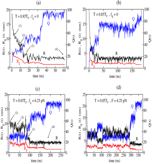
Figure 22: (a) and (b) The time dependence of $Q$, $R$ and $R_{g}$ for two typical trajectories starting from FDE ($f_{q}=0$ and $T=285$ K). The arrows 1, 2 and 3 in (a) correspond to time 3.1 ($R=10.9$ nm), 9.3 ($R=7.9$ nm) and 17.5 ns ($R=5$ nm). The arrow 4 marks the folding time $\tau_{F}$ = 62 ns ($R=2.87$ nm) when all of 99 native contacts are formed. (c) and (d) are the same as in (a) and (b) but for $f_{q}$ = 6.25 pN. The corresponding arrows refer to $t=$ 7.5 ($R=11.2$ nm), 32 ($R=9.4$ nm), 95 ns ($R=4.8$ nm) and $\tau_{F}=175$ ns ($R=3.65$ nm).

Figure 22 shows considerable diversity of refolding pathways. In accord with experiments Fernandez_Sci04 and simulations for I27 MSLi_PNAS06 , the reduction of $R$ occurs in a stepwise manner. In the $f_{q}=0$ case (Fig. 22a) $R$ decreases continuously from $\approx 18$ nm to 7.5 nm (stage 1) and fluctuates around this value for about 3 ns (stage 2). The further reduction to $R\approx 4.5$ nm (stage 3) until a transition to the NBA. The stepwise nature of variation of $Q(t)$ is also clearly shown up but it is more masked for $R_{g}(t)$. Although we can interpret another trajectory for $f_{q}=0$ (Fig. 22b) in the same way, the time scales are different. Thus, the refolding routes are highly heterogeneous.

The pathway diversity is also evident for $f_{q}>0$ (Fig. 22c and d). Although the picture remains qualitatively the same as in the $f_{q}=0$ case, the time scales for different steps becomes much larger. The molecule fluctuates around $R\approx 7$ nm, e.g., for $\approx 60$ ns (stage 2 in Fig. 22c) which is considerably longer than $\approx 3$ ns in Fig. 22a. The variation of $R_{g}(t)$ becomes more drastic compared to the $f_{q}=0$ case.

Figure 23 shows the time dependence of $<R(t)>,<Q(t)>$ and $<R_{g}(t)>$, where $<...>$ stands for averaging over 50 trajectories. The left and right panels correspond to the long and short time windows, respectively. For the TDE case (Fig. 23a and b) the single exponential fit works pretty well for $<R(t)>$ for the whole time interval. A little departure from this behavior is seen for $<Q(t)>$ and $<R_{g}(t)>$ for $t<2$ ns (Fig. 23b). Contrary to the TDE case, even for $f_{q}=0$ (Fig. 23c and d) the difference between the single and bi-exponential fits is evident not only for $<Q(t)>$ and $<R_{g}(t)>$ but also for $<R(t)>$. The time scales, above which two fits become eventually identical, are slightly different for three quantities (Fig. 23d). The failure of the single exponential behavior becomes more and more evident with the increase of $f_{q}$, as demonstrated in Figs. 23e and f for the FDE case with $f_{q}=6.25$ pN.

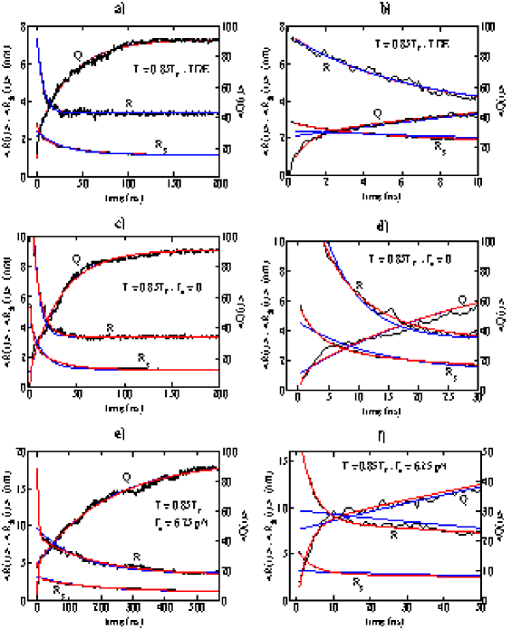
Figure 23: (a) The time dependence of $<Q(t)>$, $<R(t)>$ and $<R_{g}(t)>$ when the refolding starts from TDE. (b) The same as in (a) but for the short time scale. (c) and (d) The same as in (a) and (b) but for FDE with $f_{q}=0$. (e) and (f) The same as in (c) and (d) but for $f_{q}$=6.25 pN.

Thus, in agreement with our previous results, obtained for I27 and the sequence S1 MSLi_PNAS06 , starting from FDE the refolding kinetics compiles of the fast and slow phase. The characteristic time scales for these phases may be obtained using a sum of two exponentials,$<A(t)>=A_{0}+A_{1}\exp(-t/\tau^{A}_{1})+A_{2}\exp(-t/\tau^{A}_{2})$, where $A$ stands for $R$, $R_{g}$ or $Q$. Here $\tau^{A}_{1}$ characterizes the burst-phase (first stage) while $\tau^{A}_{2}$ may be either the collapse time (for $R$ and $R_{g}$) or the folding time (for $Q$) ($\tau^{A}_{1}<\tau^{A}_{2}$). As in the case of I27 and S1 MSLi_PNAS06 , $\tau^{R}_{1}$ and $\tau^{R_{g}}_{1}$ are almost independent on $f_{q}$ (results not shown). We attribute this to the fact that the quench force ($f_{q}^{max}\approx 9$ pN) is much lower than the entropy force ($f_{e}$) needed to stretch the protein. At $T=285$ K, one has to apply $f_{e}\approx 140$ pN for stretching Ub to 0.8 $L$. Since $f_{q}^{max}<<f_{e}$ the initial compaction of the chain that is driven by $f_{e}$ is not sensitive to the small values of $f_{q}$. Contrary to $\tau^{A}_{1}$, $\tau^{A}_{2}$ was found to increase with $f_{q}$ exponentially. Moreover, $\tau^{R}_{2}<\tau^{R_{g}}_{2}<\tau_{F}$ implying that the chain compaction occurs before the acquisition of the NS.

7.2.2 Refolding pathways of single Ubiquitin

In order to study refolding under small quenched force we follow the same protocol as in the experiments Fernandez_Sci04 . First, a large force ($\approx 130$ pN) is applied to both termini to prepare the initial stretched conformations. This force is then released, but a weak quench force, $f_{q}$, is applied to study the refolding process. The refolding of a single Ub was studied MSLi_BJ07 ; Szymczak_JCP06 in the presence or absence of the quench force. Fixing the N-terminal was found to change the refolding pathways of the free-end Ub Szymczak_JCP06 , but the effect of anchoring the C-terminal has not been studied yet. Here we study this problem in detail, monitoring the time dependence of native contacts of secondary structures (Fig. 24). Since the quench force increases the folding time but leaves the folding pathways unchanged, we present only the results for $f_{q}=0$ (Fig. 24). Interestingly, the fixed C-terminal and free-end cases have the identical folding sequencing

$$S2\rightarrow S4\rightarrow A\rightarrow S1\rightarrow(S3,S5).$$ (53)

Figure 24: The dependence of native contacts of $\beta$-strands and the helix A on the progressive variable $\delta$ when the N-terminal is fixed (a), both ends are free (b), and C-terminal is fixed (c). The results are averaged over 200 trajectories. (d) The probability of refolding pathways in three cases. each value is written on top of the histograms.

This is reverse of the unfolding pathway under thermal fluctuations MSLi_BJ07 . As discussed in detail by Li et al. MSLi_BJ07 , Eq. (53) partially agrees with the folding Went_PEDS05 and unfolding Cordier_JMB02 experiments, and simulations Fernandez_JCP01 ; Fernandez_Proteins02 ; Sorenson_Proteins02 . Our new finding here is that keeping the C-terminal fixed does not change the folding pathways. One should keep in mind that the dominant pathway given by Eq. (53) is valid in the statistical sense. It occurs in about 52% and 58% of events for the free end and C-anchored cases (Fig. 24d), respectively. The probability of observing an alternate pathway ($S2\rightarrow S4\rightarrow A\rightarrow S3\rightarrow S1\rightarrow S5)$ is $\approx 44$ % and 36 % for these two cases (Fig. 24d). The difference between these two pathways is only in sequencing of S1 and S3. Other pathways, denoted in green, are also possible but they are rather minor.

In the case when the N-terminal is fixed (Fig. 24) we have the following sequencing

$$S4\rightarrow S2\rightarrow A\rightarrow S3\rightarrow S1\rightarrow S5$$ (54)

which is, in agreement with Ref. Szymczak_JCP06, , different from the free-end case. We present folding pathways as the sequencing of secondary structures, making comparison with experiments easier than an approach based on the time evolution of individual contacts Szymczak_JCP06 . The main pathway (Eq. 54) occurs in $\approx 68$ % of events (Fig. 24d), while the competing sequencing $S4\rightarrow S2\rightarrow A\rightarrow S1\rightarrow(S1,S5)$ (28 %) and other minor pathways are also possible. From Eq. (53) and (54) it follows that the force-clamp technique can probe the folding pathways of Ub if one anchors the C-terminal but not the N-one.

In order to check the robustness of our prediction for refolding pathways (Eqs. 53 and 54), obtained for the friction $\zeta=2\frac{m}{\tau_{L}}$, we have performed simulations for the water friction $\zeta=50\frac{m}{\tau_{L}}$. Our results (not shown) demonstrate that although the folding time is about twenty times longer compared to the $\zeta=2\frac{m}{\tau_{L}}$ case, the pathways remain the same. Thus, within the framework of Go modeling, the effect of the N-terminus fixation on refolding pathways of Ub is not an artifact of fast dynamics, occurring for both large and small friction. It would be very interesting to verify our prediction using more sophisticated models. This question is left for future studies.

7.3 Refolding pathways of three-domain Ubiquitin

Figure 25: (a) The time dependence of $Q$, $R$ and $R_{g}$ at $T=285$ K for the free end case for trimer. (b) The same as in (a) but for the N-fixed case. The red line is a bi-exponential fit $A(t)=A_{0}+a_{1}\exp(-t/\tau_{1})+a_{2}\exp(-t/\tau_{2})$. Results for the C-fixed case are similar to the $N$-fixed case, and are not shown.

The time dependence of the total number of native contacts, $Q$, $R$ and the gyration radius, $R_{g}$, is presented in Fig. 25 for the trimer. The folding time $\tau_{f}\approx$ 553 ns and 936 ns for the free end and N-fixed cases, respectively. The fact that anchoring one end slows down refolding by a factor of nearly 2 implies that diffusion-collision processes Karplus_Nature76 play an important role in the Ub folding. Namely, as follows from the diffusion-collision model, the time required for formation contacts is inversely proportional to the diffusion coefficient, $D$, of a pair of spherical units. If one of them is idle, $D$ is halved and the time needed to form contacts increases accordingly. The similar effect for unfolding was observed in our recent work MSLi_BJ07 .

From the bi-exponential fitting, we obtain two time scales for collapsing ($\tau_{1}$) and compaction ($\tau_{2}$) where $\tau_{1}<\tau_{2}$. For $R$, e.g., $\tau_{1}^{R}\approx 2.4$ ns and $\tau_{2}^{R}\approx 52.3$ ns if two ends are free, and $\tau_{1}^{R}\approx 8.8$ ns and $\tau_{2}^{R}\approx 148$ ns for the fixed-N case. Similar results hold for the time evolution of $R_{g}$. Thus, the collapse is much faster than the barrier limited folding process. Monitoring the time evolution of $\Delta R$ and of the number of native contacts, one can show (results not shown) that the refolding of the trimer is staircase-like as observed in the simulations Best_Science05 ; MSLi_BJ07 and the experiments Fernandez_Sci04 .

Figure 26: The same as in Fig. 24 but for the trimer. The numbers 1, 2 and 3 refer to the first, second and third domain. The last row represents the results averaged over three domains. The fractions of native contacts of each secondary structure are averaged over 100 trajectories.

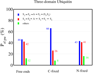
Figure 27: (a) The probability of different refolding pathways for the trimer. Each value is shown on top of the histograms.

Fig. 26 shows the dependence of the number of native contacts of the secondary structures of each domain on $\delta$ for three situations: both termini are free and one or the other of them is fixed. In each of these cases the folding pathways of three domains are identical. Interestingly, they are the same, as given by Eq. (53), regardless of we keep one end fixed or not. As evident from Fig. 27, although the dominant pathway is the same for three cases its probabilities are different. It is equal 68%, 44% and 43% for the C-fixed, free-end and N-fixed cases, respectively. For the last two cases, the competing pathway S${}_{2}\rightarrow$ S${}_{4}\rightarrow$ A $\rightarrow$ S${}_{3}\rightarrow$ S${}_{1}\rightarrow$ S₅ has a reasonably high probability of $\approx$ 40%.

The irrelevance of one-end fixation for refolding pathways of a multi-domain Ub may be understood as follows. Recall that applying the low quenched force to both termini does not change folding pathways of single Ub MSLi_BJ07 . So in the three-domain case, with the N-end of the first domain fixed, both termini of the first and second domains are effectively subjected to external force, and their pathways should remain the same as in the free-end case. The N-terminal of the third domain is tethered to the second domain but this would have much weaker effect compared to the case when it is anchored to a surface. Thus this unit has almost free ends and its pathways remain unchanged. Overall, the ”boundary” effect gets weaker as the number of domains becomes bigger. In order to check this argument, we have performed simulations for the two-domain Ub. It turns out that the sequencing is roughly the same as in Fig. 26, but the common tendency is less pronounced (results not shown) compared to the trimer case. Thus we predict that the force-clamp technique can probe folding pathways of free Ub if one uses either the single domain with the C-terminus anchored, or the multi-domain construction.

Figure 28: The dependence of the total number of native contacts on $\delta$ for the first (green), second (red) and third (blue) domains. Typical snapshots of the initial, middle and final conformations for three cases when both two ends are free or one of them is fixed. The effect of anchoring one terminus on the folding sequencing of domains is clearly evident. In the bottom we show the probability of refolding pathways for three cases. Its value is written on the top of histograms.

Although fixing one end of the trimer does not influence folding pathways of individual secondary structures, it affects the folding sequencing of individual domains (Fig. 28). We have the following sequencing $(1,3)\rightarrow 2$, $3\rightarrow 2\rightarrow 1$ and $1\rightarrow 2\rightarrow 3$ for the free-end, N-terminal fixed and C-terminal fixed, respectively. These scenarios are supported by typical snapshots shown in Fig. 28. It should be noted that the domain at the free end folds first in all of three cases in statistical sense (also true for the two-domain case). As follows from the bottom of Fig. 28, if two ends are free then each of them folds first in about 40 out of 100 observations. The middle unit may fold first, but with much lower probability of about 15%. This value remains almost unchanged when one of the ends is anchored, and the probability that the non-fixed unit folds increases to $\geq 80$%.

7.4 Is the effect of fixing one terminus on refolding pathways universal?

We now ask if the effect of fixing one end on refolding pathway, observed for Ub, is also valid for other proteins? To answer this question, we study the single domain I27 from the muscle protein titin. We choose this protein as a good candidate from the conceptual point of view because its $\beta$-sandwich structure (see Fig. 29a) is very different from $\alpha/\beta$-structure of Ub.

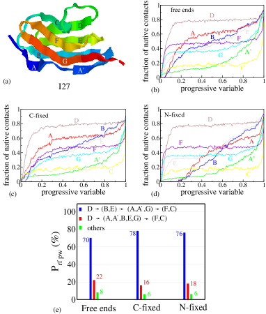
Figure 29: (a) NS conformation of Ig27 domain of titin(PDB ID: 1tit). There are 8 $\beta$-strands: A (4-7), A’ (11-15), B (18-25), C (32-36), D (47-52), E (55-61), F(69-75) and G (78-88). The dependence of native contacts of different $\beta$-strands on the progressive variable $\delta$ for the case when two ends are free (b), the N-terminus is fixed (c) and the C-terminal is anchored (d). (e) The probability of observing refolding pathways for three cases. Each value is written on top of the histograms.

Moreover, because I27 is subject to mechanical stress under physiological conditions Erickson_Science97 , it is instructive to study refolding from extended conformations generated by force. There have been extensive unfolding (see recent review Sotomayor_Science07 for references) and refolding MSLi_PNAS06 studies on this system, but the effect of one-end fixation on folding sequencing of individual secondary structures have not been considered either theoretically or experimentally.

As follows from Fig. 29b, if two ends are free then strands A, B and E fold at nearly the same rate. The pathways of the N-fixed and C-fixed cases are identical, and they are almost the same as in the free end case except that the strand A seems to fold after B and E. Thus, keeping the N-terminus fixed has much weaker effect on the folding sequencing as compared to the single Ub. Overall the effect of anchoring one terminus has a little effect on the refolding pathways of I27, and we have the following common sequencing

$$D\rightarrow(B,E)\rightarrow(A,G,A^{\prime})\rightarrow F\rightarrow C$$ (55)

for all three cases. The probability of observing this main pathways varies between 70 and 78% (Fig. 29e). The second pathway, D $\rightarrow$ (A,A’,B,E,G) $\rightarrow$ (F,C), has considerably lower probability. Other minor routes to the NS are also possible.

Because the multi-domain construction weakens this effect, we expect that the force-clamp spectroscopy can probe refolding pathways for a single and poly-I27. More importantly, our study reveals that the influence of fixation on refolding pathways may depend on the native topology of proteins.

7.5 Free energy landscape

Figure 30 shows the dependence of the folding times on $f_{q}$. Using the Bell-type formula (Eq. 29) and the linear fit in Fig. 30, we obtain $x_{f}=0.96\pm 0.15$ nm which is in acceptable agreement with the experimental value $x_{f}\approx 0.8$ nm Fernandez_Sci04 .

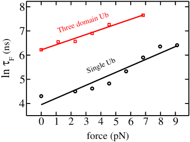
Figure 30: The dependence of folding times on the quench force at $T=285$ K. $\tau_{F}$ was computed as the average of the first passage times ($\tau_{F}$ is the same as $\tau^{Q}_{2}$ extracted from the bi-exponential fit for $<Q(t)>$). The result is averaged over 30 - 50 trajectories for each value of $f_{q}$. From the linear fits $y=3.951+0.267x$ and $y=6.257+0.207x$ we obtain $x_{f}=0.96\pm 0.15$ nm for single Ub (black circles and curve) and $x_{f}=0.74\pm 0.07$ nm for trimer (red squares and curve), respectively.

The linear growth of the free energy barrier to folding with $f_{q}$ is due to the stabilization of the random coil states under the force. Our estimate for Ub is higher than $x_{f}\approx 0.6$ nm obtained for I27 MSLi_PNAS06 . One of possible reasons for such a pronounced difference is that we used the cutoff distance $d_{c}=0.65$ and 0.6 nm in the Go model for Ub and I27, respectively. The larger value of $d_{c}$ would make a protein more stable (more native contacts) and it may change the FEL leading to enhancement of $x_{f}$. This problem requires further investigation.

From Fig. 30 we obtain $x_{f}=0.74\pm 0.07$ nm for trimer. Within the error bars this value coincides with $x_{f}=0.96\pm 0.15$ nm for Ub, and also with the experimental result $x_{f}\approx 0.80$ nm Fernandez_Sci04 . Our results suggest that the multi-domain structure leaves $x_{f}$ almost unchanged.

7.6 Conclusions

We have shown that, in agreement with the experiments Fernandez_Sci04 , refolding of Ub under quenched force proceeds in a stepwise manner. The effect of the one-terminal fixation on refolding pathways depends on individual protein and it gets weaker by a multi-domain construction. Our theoretical estimate of $x_{f}$ for single Ub is close to the experimental one and it remains almost the same for three-domain case.

Chapter 8 Mechanical and thermal unfolding of single and three domain Ubiquitin

8.1 Introduction

Experimentally, the unfolding of the poly-Ub has been studied by applying a constant force Schlierf_PNAS04 . The mechanical unfolding of Ub has previously investigated using Go-like West_BJ06 and all-atom models West_BJ06 ; Irback_PNAS05 . In particular, Irbäck et al. have explored mechanical unfolding pathways of structures A, B, C, D and E (see the definition of these structures and the $\beta$-strands in the caption to Fig. 17) and the existence of intermediates in detail. We present our results on mechanical unfolding of Ub for five following reasons.

1. The barrier to the mechanical unfolding has not been computed.

2. Experiments of Schlierf et al. Schlierf_PNAS04 have suggested that cluster 1 (strands S1, S2 and the helix A) unfolds after cluster 2 (strands S3, S4 and S5). However, this observation has not yet been studied theoretically.

3. Since the structure C, which consists of the strands S1 and S5, unzips first, Irbäck et al. pointed out that the strand S5 unfolds before S2 or the terminal strands follows the unfolding pathway S1 $\rightarrow$ S5 $\rightarrow$ S2. This conclusion may be incorrect because it has been obtained from the breaking of the contacts within the structure C.

4. In pulling and force-clamp experiments the external force is applied to one end of proteins whereas the other end is kept fixed. Therefore, one important question emerges is how fixing one terminus affects the unfolding sequencing of Ub. This issue has not been addressed by Irbäck et al. Irback_PNAS05 .

5. Using a simplified all-atom model it was shown Irback_PNAS05 that mechanical intermediates occur more frequently than in experiments Schlierf_PNAS04 . It is relevant to ask if a C_α-Go model can capture similar intermediates as this may shed light on the role of non-native interactions.

From the force dependence of mechanical unfolding times, we estimated the distance between the NS and the TS to be $x_{u}\approx 0.24$ nm which is close to the experimental results of Carrion-Vazquez et al. Carrion-Vazquez_NSB03 and Schlierf et al. Schlierf_PNAS04 . In agreement with the experiments Schlierf_PNAS04 , cluster 1 was found to unfold after cluster 2 in our simulations. Applying the force to the both termini, we studied the mechanical unfolding pathways of the terminal strands in detail and obtained the sequencing S1 $\rightarrow$ S2 $\rightarrow$ S5 which is different from the result of Irbäck et al.. When the N-terminus is fixed and the C-terminus is pulled by a constant force the unfolding sequencing was found to be very different from the previous case. The unzipping initiates, for example, from the C-terminus but not from the N-one. Anchoring the C-end is shown to have a little effect on unfolding pathways. We have demonstrated that the present C_α-Go model does not capture rare mechanical intermediates, presumably due to the lack of non-native interactions. Nevertheless, it can correctly describe the two-state unfolding of Ub Schlierf_PNAS04 .

It is well known that thermal unfolding pathways may be very different from the mechanical ones, as has been shown for the domain I27 Paci_PNAS00 . This is because the force is applied locally to the termini while thermal fluctuations have the global effect on the entire protein. In the force case unzipping should propagate from the termini whereas under thermal fluctuations the most unstable part of a polypeptide chain unfolds first.

The unfolding of Ub under thermal fluctuations was investigated experimentally by Cordier and Grzesiek Cordier_JMB02 and by Chung et al. Chung_PNAS05 . If one assumes that unfolding is the reverse of the refolding process then one can infer information about the unfolding pathways from the experimentally determined $\phi$-values Went_PEDS05 and $\psi$-values Krantz_JMB04 ; Sosnick_ChemRev06 . The most comprehensive $\phi$-value analysis is that of Went and Jackson. They found that the C-terminal region which has very low $\phi$-values unfolds first and then the strand S1 breaks before full unfolding of the $\alpha$ helix fragment A occurs. However, the detailed unfolding sequencing of the other strands remains unknown.

Theoretically, the thermal unfolding of Ub at high temperatures has been studied by all-atom MD simulations by Alonso and Daggett Alonso_ProSci98 and Larios et al. Larios_JMB04 . In the latter work the unfolding pathways were not explored. Alonso and Daggett have found that the $\alpha$-helix fragment A is the most resilient towards temperature but the structure B breaks as early as the structure C. The fact that B unfolds early contradicts not only the results for the $\phi$-values obtained experimentally by Went and Jackson Went_PEDS05 but also findings from a high resolution NMR Cordier_JMB02 . Moreover, the sequencing of unfolding events for the structures D and E was not studied.

What information about the thermal unfolding pathways of Ub can be inferred from the folding simulations of various coarse-grained models? Using a semi-empirical approach Fernandez predicted Fernandez_JCP01 that the nucleation site involves the $\beta$-strands S1 and S5. This suggests that thermal fluctuations break these strands last but what happens to the other parts of the protein remain unknown. Furthermore, the late breaking of S5 contradicts the unfolding Cordier_JMB02 and folding Went_PEDS05 experiments. From later folding simulations of Fernandez et al. Fernandez_Proteins02 ; Fernandez_PhysicaA02 one can infer that the structures A, B and C unzip late. Since this information is gained from $\phi$-values, it is difficult to determine the sequencing of unfolding events even for these fragments. Using the results of Gilis and Rooman Gilis_Proteins01 we can only expect that the structures A and B unfold last. In addition, with the help of a three-bead model it was found Sorenson_Proteins02 that the C-terminal loop structure is the last to fold in the folding process and most likely plays a spectator role in the folding kinetics. This implies that the strands S4, S5 and the second helix (residues 38-40) would unzip first but again the full unfolding sequencing can not be inferred from this study.

Thus, neither the direct MD Alonso_ProSci98 nor indirect folding simulations Fernandez_JCP01 ; Fernandez_Proteins02 ; Fernandez_PhysicaA02 ; Gilis_Proteins01 ; Sorenson_Proteins02 provide a complete picture of the thermal unfolding pathways for Ub. One of our aims is to decipher the complete thermal unfolding sequencing and compare it with the mechanical one. The mechanical and thermal routes to the DSs have been found to be very different from each other. Under the force the $\beta$-strand S1, e.g., unfolds first, while thermal fluctuations detach strand S5 first. The later observation is in good agreement with NMR data of Cordier and Grzesiek Cordier_JMB02 . A detailed comparison with available experimental and simulation data on the unfolding sequencing will be presented. The free energy barrier to thermal unfolding was also calculated.

Another part of this chapter was inspired by the recent pulling experiments of Yang et al. Yang_RSI06 . Performing the experiments in the temperature interval between 278 and 318 K, they found that the unfolding force (maximum force in the force-extension profile), $f_{u}$, of Ub depends on temperature linearly. In addition, the corresponding slopes of the linear behavior have been found to be independent of pulling velocities. An interesting question that arises is if the linear dependence of $f_{u}$ on $T$ is valid for this particular region, or it holds for the whole temperature interval. Using the same Go model Clementi_JMB00 , we can reproduce the experimental results of Yang et al. Yang_RSI06 on the quasi-quantitative level. More importantly, we have shown that for the entire temperature interval the dependence is not linear, because a protein is not an entropic spring in the temperature regime studied.

We have studied the effect of multi-domain construction and linkage on the location of the TS along the end-to-end distance reaction coordinate, $x_{u}$. It is found that the multi-domain construction has a minor effect on $x_{u}$ but, in agreement with the experiments Carrion-Vazquez_NSB03 , the Lys48-C linkage has the strong effect on it. Using the microscopic theory for unfolding dynamics Dudko_PRL06 , we have determined the unfolding barrier for Ub.

This chapter is based on the results presented in Refs. MSLi_BJ07 ; Kouza_JCP08 .

8.2 Materials and Methods

We use the Go-like model (Eq. 5) for the single as well as multi-domain Ub. It should be noted that the folding thermodynamics does not depend on the environment viscosity (or on $\zeta$) but the folding kinetics depends on it. Most of our simulations (if not stated otherwise) were performed at the friction $\zeta=2\frac{m}{\tau_{L}}$, where the folding is fast. The equations of motion were integrated using the velocity form of the Verlet algorithm Swope_JCP82 with the time step $\Delta t=0.005\tau_{L}$ (Chapter 3). In order to check the robustness of our predictions for refolding pathways, limited computations were carried out for the friction $\zeta=50\frac{m}{\tau_{L}}$ which is believed to correspond to the viscosity of water Veitshans_FD97 ). In this overdamped limit we use the Euler method (Eq. 20) for integration and the time step $\Delta t=0.1\tau_{L}$.

The progressive variable $\delta$ (Eq. 31) was used to probe folding pathways. In the constant velocity force simulation, we fix the N-terminal and follow the procedure described in Section 3.1.2. The pulling speeds are set equal $\nu=3.6\times 10^{7}$ nm/s and 4.55 $\times 10^{8}$ nm/s which are about 5 - 6 orders of magnitude faster than those used in experiments Yang_RSI06 .

8.3 Mechanical unfolding pathways

8.3.1 Absence of mechanical unfolding intermediates in C_α-Go model

In order to study the unfolding dynamics of Ub, Schlierf et al. Schlierf_PNAS04 have performed the AFM experiments at a constant force $f=100,140$ and 200 pN. The unfolding intermediates were recorded in about $5\%$ of 800 events at different forces. The typical distance between the initial and intermediate states is $\Delta R=8.1\pm 0.7$ nm Schlierf_PNAS04 . However, the intermediates do not affect the two-state behavior of the polypeptide chain. Using the all-atom models Irbäck et al. Irback_PNAS05 have also observed the intermediates in the region 6.7 nm $<R<18.5$ nm. Although the percentage of intermediates is higher than in the experiments, the two-state unfolding events remain dominating. To check the existence of force-induced intermediates in our model, we have performed the unfolding simulations for $f=70,100,140$ and 200 pN. Because the results are qualitatively similar for all values of force, we present $f=100$ pN case only.

Figure 31a shows the time dependence of $R(t)$ for fifteen runs starting from the native value $R_{N}\approx 3.9$ nm. For all trajectories the plateau occurs at $R\approx 4.4$ nm. As seen below, passing this plateau corresponds to breaking of intra-structure native contacts of structure C. At this stage the chain ends get almost stretched out, but the rest of the polypeptide chain remains native-like. The plateau is washed out when we average over many trajectories and $<R(t)>$ is well fitted by a single exponential (Fig. 31a), in accord with the two-state behavior of Ub Schlierf_PNAS04 .

The existence of the plateau observed for individual unfolding events in Fig. 31a agrees with the all-atom simulation results of Irbäck et al. Irback_PNAS05 who have also recorded the similar plateau at $R\approx 4.6$ nm at short time scales. However unfolding intermediates at larger extensions do not occur in our simulations. This is probably related to neglect of the non-native interactions in the C_α-Go model. Nevertheless, this simple model provides the correct two-state unfolding picture of Ub in the statistical sense.

8.3.2 Mechanical unfolding pathways: force is applied to both termini

Here we focus on the mechanical unfolding pathways by monitoring the number of native contacts as a function of the end-to-end extension $\Delta R\equiv R-R_{\rm eq}$, where $R_{\rm eq}$ is the equilibrium value of $R$. For $T=285$ K, $R_{\rm eq}\approx 3.4$ nm. Following Schlierf et al. Schlierf_PNAS04 , we first divide Ub into two clusters. Cluster 1 consists of strands S1, S2 and the helix A (42 native contacts) and cluster 2 - strands S3, S4 and S5 (35 native contacts). The dependence of fraction of intra-cluster native contacts is shown in Fig. 31b for $f=70$ and 200 pN (similar results for $f=100$ and 140 pN are not shown). In agreement with the experiments Schlierf_PNAS04 the cluster 2 unfolds first. The unfolding of these clusters becomes more and more synchronous upon decreasing $f$. At $f=70$ pN the competition with thermal fluctuations becomes so important that two clusters may unzip almost simultaneously. Experiments at low forces are needed to verify this observation.

Figure 31: (a) Time dependence of the end-to-end distance for $f=100$ pN. The thin curves refer to fifteen representative trajectories. The averaged over 200 trajectory $<R(t)>$ is represented by the thick line. The dashed curve is the single exponential fit $<R(t)>=21.08-16.81\exp(-x/\tau_{u})$, where $\tau_{u}\approx 11.8$ ns. (b) The dependence of fraction of the native contacts on $\Delta R$ for cluster 1 (solid lines) and cluster 2 (dashed lines) at $f=70pN$ and 200 pN. The results are averaged over 200 independent trajectories. The arrow points to $\Delta R$ = 8.1 nm.

The arrow in Fig. 31b marks the position $\Delta R=8.1$ nm, where some intermediates were recorded in the experiments Schlierf_PNAS04 . At this point there is intensive loss of native contacts of the cluster 2 suggesting that the intermediates observed on the experiments are conformations in which most of the contacts of this cluster are already broken but the cluster 1 remains relatively structured ($\approx 40\%$ contacts). One can expect that the cluster 1 is more ordered in the intermediate conformations if the side chains and realistic interactions between amino acids are taken into account.

To compare the mechanical unfolding pathways of Ub with the all-atom simulation results Irback_PNAS05 we discuss the sequencing of helix A and structures B, C, D and E in more detail. We monitor the intra-structure native contacts and all contacts separately. The later include not only the contacts within a given structure but also the contacts between it and the rest of the protein. It should be noted that Irbäck et al. have studied the unfolding pathways based on the evolution of the intra-structure contacts. Fig. 32a shows the dependence of the fraction of intra-structure contacts on $\Delta R$ at $f=100$ pN. At $\Delta R\approx$ 1nm, which corresponds to the plateau in Fig. 31a, most of the contacts of C are broken. In agreement with the all-atom simulations Irback_PNAS05 , the unzipping follows C $\rightarrow$ B $\rightarrow$ D $\rightarrow$ E $\rightarrow$ A. Since C consists of the terminal strands S1 and S5, it was suggested that these fragments unfold first. However, this scenario may be no longer valid if one considers not only intra-structure contacts but also other possible ones (Fig. 32b). In this case the statistically preferred sequencing is B $\rightarrow$ C $\rightarrow$ D $\rightarrow$ E $\rightarrow$ A which holds not only for $f$=100 pN but also for other values of $f$. If it is true then S2 unfold even before S5. To make this point more transparent, we plot the fraction of contacts for S1, S2 and S5 as a function of $\Delta R$ (Fig. 32c) for a typical trajectory. Clearly, S5 detaches from the core part of a protein after S2 (see also the snapshot in Fig. 32d). So, instead of the sequencing S1 $\rightarrow$ S5 $\rightarrow$ S2 proposed by Irbäck et al., we obtain S1 $\rightarrow$ S2 $\rightarrow$ S5.

Figure 32: (a) The dependence of fraction of the intra-structure native contacts on $\Delta R$ for structures A, B, C, D and E at $f=100$ pN. (b) The same as in a) but for all native contacts. (c) The dependence of fraction of the native contacts on $\Delta R$ for strand S1, S2 and S5 ($f=200pN$). The vertical dashed line marks the position of the plateau at $\Delta R\approx$ 1 nm. (d) The snapshot, chosen at the extension marked by the arrow in c), shows that S2 unfolds before S5. At this point all native contacts of S1 and S2 have already broken while 50$\%$ of the native contacts of S5 are still present. (e) The dependence of fraction of the native contacts on extension for A and all $\beta$-strands at $f=70pN$. (f) The same as in e) but for $f=200$ pN. The arrow points to $\Delta R=8.1$ nm where the intermediates are recorded on the experiments Schlierf_PNAS04 . The results are averaged over 200 trajectories.

The dependence of the fraction of native contacts on $\Delta R$ for individual strands is shown in Fig. 32e ($f=70$ pN) and Fig. 32f ($f$=200 pN). At $\Delta=8.1$ nm contacts of S1, S2 and S5 are already broken whereas S4 and A remain largely structured. In terms of $\beta$-strands and A we can interpret the intermediates observed in the experiments of Schlierf et al. Schlierf_PNAS04 as conformations with well structured S4 and A, and low ordering of S3. This interpretation is more precise compared to the above argument based on unfolding of two clusters because if one considers the average number of native contacts, then the cluster 2 is unstructured in the IS (Fig. 31b, but its strand S4 remains highly structured (Figs. 32e-f).

From Figs. 32e-f we obtain the following mechanical unfolding sequencing

$${\rm S1}\rightarrow{\rm S2}\rightarrow{\rm S5}\rightarrow{\rm S3}\rightarrow{\rm S4}\rightarrow{\rm A}.$$ (56)

It should be noted that the sequencing (56) is valid in the statistical sense. In some trajectories S5 unfolds even before S1 and S2 or the native contacts of S1, S2 and S5 may be broken at the same time scale (Table 4).

Force (pN)	S1 $\rightarrow$ S2 $\rightarrow$ S5 ($\%$)	S5 $\rightarrow$ S1 $\rightarrow$ S2 ($\%$)	(S1,S2,S5) ($\%$)
70	81	8	11
100	76	10	14
140	53	23	24
200	49	26	25

Table 4: Dependence of unfolding pathways on the external force. There are three possible scenarios: S1 $\rightarrow$ S2 $\rightarrow$ S5, S5 $\rightarrow$ S1 $\rightarrow$ S2, and three strands unzip almost simultaneously (S1,S2,S5). The probabilities of observing these events are given in percentage.

From the Table 4 it follows that the probability of having S1 unfolded first decreases with lowering $f$ but the main trend Eq. (56) remains unchanged. One has to stress again that the sequencing of the terminal strands S1, S2 and S5 given by Eq. (56) is different from what proposed by Irbäck et al. based on the breaking of the intra-structure contacts of C. Unfortunately, there are no experimental data available for comparison with our theoretical prediction.

8.3.3 Mechanical unfolding pathways: One end is fixed

N-terminus is fixed. Here we adopted the same procedure as in the previous section except the N-terminus is held fixed during simulations. As in the process where both of the termini are subjected to force, one can show that the cluster 1 unfolds after the cluster 2 (results not shown).

From Fig. 33 we obtain the following unfolding pathways

$${\rm C}\rightarrow{\rm D}\rightarrow{\rm E}\rightarrow{\rm B}\rightarrow{\rm A},$$ (57a)

$${\rm S5}\rightarrow{\rm S3}\rightarrow{\rm S4}\rightarrow{\rm S1}\rightarrow{\rm S2}\rightarrow{\rm A},$$ (57b)

which are also valid for the other values of force ($f$=70, 100 and 140 pN). Similar to the case when the force is applied to both ends, the structure C unravels first and the helix A remains the most stable. However, the sequencing of B, D and E changes markedly compared to the result obtained by Irbäck et al Irback_PNAS05 (Fig. 32a).

Figure 33: (a) The dependence of fraction of the intra-structure native contacts on extension for all structures at $f=200pN$. The N-terminus is fixed and the external force is applied via the C-terminus. (b) The same as in (a) but for the native contacts of all individual $\beta$-strands and helix A . The results are averaged over 200 trajectories. (c) A typical snapshot which shows that S₅ is fully detached from the core while S₁ and S₂ still have $\approx 50\%$ and 100% contacts, respectively. (d) The same as in (b) but the C-end is anchored and N-end is pulled. The strong drop in the fraction of native contacts of S₄ at $\Delta R\approx 7.5$ nm does not correspond to the substantial change of structure as it has only 3 native contacts in total.

As evident from Eqs. 56 and 57b, anchoring the first terminal has a much more pronounced effect on the unfolding pathways of individual strands. In particular, unzipping commences from the C-terminus instead of from the N-one. Fig. 33c shows a typical snapshot where one can see clearly that S₅ detaches first. At the first glance, this fact may seem trivial because S₅ experiences the external force directly. However, our experience on unfolding pathways of the well studied domain I27 from the human cardiac titin, e.g., shows that it may be not the case. Namely, as follows from the pulling experiments Marszalek_Nature99 and simulations Lu_Proteins99 , the strand A from the N-terminus unravels first although this terminus is kept fixed. From this point of view, what strand of Ub detaches first is not a priory clear. In our opinion, it depends on the interplay between the native topology and the speed of tension propagation. The later factor probably plays a more important role for Ub while the opposite situation happens with I27. One of possible reasons is related to the high stability of the helix A which does not allow either for the N-terminal to unravel first or for seriality in unfolding starting from the C-end.

C-terminus is fixed. One can show that unfolding pathways of structures A,B, C, D and E remain exactly the same as in the case when Ub has been pulled from both termini (see Fig. 32a-b). Concerning the individual strands, a slight difference is observed for S₅ (compare Fig. 33d and Fig. 32e). Most of the native contacts of this domain break before S₃ and S₄, except the long tail at extension $\Delta R\gtrsim$ 11 nm due to high mechanical stability of only one contact between residues 61 and 65 (the highest resistance of this pair is probably due to the fact that among 25 possible contacts of S₅ it has the shortest distance $|61-65|=4$ in sequence). This scenario holds in about 90% of trajectories whereas S₅ unravels completely earlier than S₃ and S₄ in the remaining trajectories. Thus, anchoring C-terminus has much less effect on unfolding pathways compared to the case when the N-end is immobile.

It is worthwhile to note that, experimentally one has studied the effect of extension geometry on the mechanical stability of Ub fixing its C-terminus Carrion-Vazquez_NSB03 . The greatest mechanical strength (the longest unfolding time) occurs when the protein is extended between N- and C-termini. This result has been supported by Monte Carlo Carrion-Vazquez_NSB03 as well as MD West_BJ06 simulations. However the mechanical unfolding sequencing has not been studied yet. It would be interesting to check our results on the effect of fixing one end on Ub mechanical unfolding pathways by experiments.

8.4 Free energy landscape

In experiments one usually uses the Bell formula Bell_Sci78 (Eq. 24) to extract $x_{u}$ for two-state proteins from the force dependence of unfolding times. This formula is valid if the location of the TS does not move under external force. However, under external force the TS moves toward NS. In this case, one can use Eq. (28) to estimate not only $x_{u}$ but also $G^{\ddagger}$ for $\nu=1/2$ and 2/3. This will be done in this section for the single Ub and the trimer.

Figure 34: The semi-log plot for the force dependence of unfolding times at $T=285$ K. Crosses and squares refer the the single Ub and the trimer with the force applied to N- and C-terminal, respectively. Circles refer to the single Ub with the force applied to Lys48 and C-terminal. Depending on $f$, 30-50 folding events were using for averaging. In the Bell approximation, if the N- and C-terminal of the trimer are pulled then we have the linear fit $y=10.448-0.066x$ (black line) and $x_{u}\approx$ 0.24 nm. The same value of $x_{u}$ was obtained for the single Ub MSLi_BJ07 . In the case when we pull at Lys48 and C-terminal of single Ub the linear fit (black line) at low forces is $y=11.963-0.168x$ and $x_{u}=0.61$ nm. The correlation level of fitting is about 0.99. The red and blue curves correspond to the fits with $\nu=1/2$ and $2/3$, respectively (Eq. 63).

8.4.1 Single Ub

Using the Bell approximation and Fig. 34, we have $x_{u}\approx 2.4\AA\,$ MSLi_BJ07 ; Kouza_JCP08 which is consistent with the experimental data $x_{u}=1.4-2.5$ ÅCarrion-Vazquez_NSB03 ; Schlierf_PNAS04 ; Chyan_BJ04 . With the help of an all-atom simulation Li et al. Li_JCP04 have shown that $x_{u}$ does depend on $f$. At low forces, where the Bell approximation is valid MSLi_BJ07 , they obtained $x_{u}=10$ Å, which is noticeably higher than our and the experimental value. Presumably, this is due to the fact that these authors computed $x_{u}$ from equilibrium data, but their sampling was not good enough for such a long protein as Ub.

We now use Eq. (63) with $\nu=2/3$ and $\nu=1/2$ to compute $x_{u}$ and $\Delta G^{\ddagger}$. The regions, where the $\nu=2/3$ and $\nu=1/2$ fits works well, are wider than that for the Bell scenario (Fig. 34). However these fits can not to cover the entire force interval. The values of $\tau_{u}^{0},x_{u}$ and $\Delta G^{\ddagger}$ obtained from the fitting procedure are listed in Table 5. According to Ref. Dudko_PRL06, , all of these quantities increase with decreasing $\nu$. In our opinion, the microscopic theory ($\nu=2/3$ and $\nu=1/2$) gives too high a value for $x_{u}$ compared to its typical experimental value Carrion-Vazquez_NSB03 ; Schlierf_PNAS04 ; Chyan_BJ04 . However, the latter was calculated from fitting experimental data to the Bell formula, and it is not clear how much the microscopic theory would change the result.

	Ub			Lys48-C			trimer
$\nu$	1/2	2/3	1	1/2	2/3	1	1/2	2/3	1
$\quad\tau_{U}^{0}(\mu s)\quad$	13200	1289	9.1	4627	2304	157	1814	756	47
$x_{u}(\AA)\quad$	7.92	5.86	2.4	12.35	10.59	6.1	6.21	5.09	2.4
$\quad\Delta G^{\ddagger}(k_{B}T)\quad$	17.39	14.22	-	15.90	13.94	-	13.49	11.64	-

Table 5: Dependence of $x_{u}$ on fitting procedures for the three-domain Ub and Lys48-C. $\nu=1$ corresponds to the phenomenological Bell approximation (Eq. 24). $\nu=1/2$ and 2/3 refer to the microscopic theory (Eq. 63). For Ub and trimer the force is applied to both termini.

In order to estimate the unfolding barrier of Ub from the available experimental data and compare it with our theoretical estimate, we use the following formula

$$\Delta G^{\ddagger}=-k_{B}T\ln(\tau_{A}/\tau_{u}^{0})$$ (58)

where $\tau_{u}^{0}$ denotes the unfolding time in the absence of force and $\tau_{A}$ is a typical unfolding prefactor. Since $\tau_{A}$ for unfolding is not known, we use the typical value for folding $\tau_{A}=1\mu$s MSLi_Polymer04 ; Schuler_Nature02 . Using $\tau_{u}^{0}=10^{4}/4$ s Khorasanizadeh_Biochem93 and Eq. (58) we obtain $\Delta G^{\ddagger}=21.6k_{B}T$ which is in reasonable agreement with our result $\Delta G^{\ddagger}\approx 17.4k_{B}T$, followed from the microscopic fit with $\nu=1/2$. Using the GB/SA continuum solvation model Qiu_JPCA97 and the CHARMM27 force field MacKerell_JPCB98 Li and Makarov Li_JCP04 ; Li_JPCB04 obtained a much higher value $\Delta G^{\ddagger}=29$ kcal/mol $\approx 48.6k_{B}T$. Again, the large departure from the experimental result may be related to poor sampling or to the force filed they used.

8.4.2 The effect of linkage on $x_{u}$ for single Ub

One of the most interesting experimental results of Carrion-Vazquez et al.Carrion-Vazquez_NSB03 is that pulling Ub at different positions changes $x_{u}$ drastically. Namely, if the force is applied at the C-terminal and Lys48, then in the Bell approximation $x_{u}\approx 6.3$ Å, which is about two and half times larger than the case when the termini N and C are pulled. Using the all-atom model Li and Makarov Li_JCP04 have shown that $x_{u}$ is much larger than 10 Å. Thus, a theoretical reliable estimate for $x_{u}$ of Lys48-C Ub is not available. Our aim is to compute $x_{u}$ employing the present Go-like model Clementi_JMB00 as it is successful in predicting $x_{u}$ for the N-C Ub. Fig. 34 shows the force dependence of unfolding time of the fragment Lys48-C when the force is applied to Lys48 and C-terminus. The unfolding time is defined as the averaged time to stretch this fragment. From the linear fit ($\nu=1$ in Fig. 34) at low forces we obtain $x_{u}\approx 0.61$ nm which is in good agreement with the experiment Carrion-Vazquez_NSB03 . The Go model is suitable for estimating $x_{u}$ for not only Ub, but also for other proteins MSLi_BJ07a because the unfolding is mainly governed by the native topology. The fact that $x_{u}$ for the linkage Lys48-C is larger than that of the N-C Ub may be understood using our recent observation MSLi_BJ07a that it anti-correlates with the contact order (CO) Plaxco_JMB98 . Defining contact formation between any two amino acids ($|i-j|\geq 1$) as occurring when the distance between the centers of mass of side chains $d_{ij}\leq 6.0$ Å(see also $http://depts.washington.edu/bakerpg/contact$_$order/$), we obtain CO equal 0.075 and 0.15 for the Lys48-C and N-C Ub, respectively. Thus, $x_{u}$ of the Lys48-C linkage is larger than that of the N-C case because its CO is smaller. This result suggests that the anti-correlation between $x_{u}$ and CO may hold not only when proteins are pulled at termini MSLi_BJ07a , but also when the force is applied to different positions. Note that the linker (not linkage) effect on $x_{u}$ has been studied for protein L West_PRE06 . It seems that this effect is less pronounced compared the effect caused by changing pulling direction studied here. We have carried out the microscopic fit for $\nu=1/2$ and $2/3$ (Fig. 34). As in the N-C Ub case, $x_{u}$ is larger than its Bell value. However the linkage at Lys48 has a little effect on the activation energy $\Delta G^{\ddagger}$ (Table 5).

8.4.3 Determination of $x_{u}$ for the three-domain ubiquitin

Since the trimer is a two-state folder (Fig. 20c), one can determine its averaged distance between the NS and TS, $x_{u}$, along the end-to-end distance reaction coordinate using kinetic theory Bell_Sci78 ; Dudko_PRL06 . We now ask if the multi-domain structure of Ub changes $x_{u}$. As in the single Ub case MSLi_BJ07 , there exists a critical force $f_{c}\approx 120$pN separating the low force and high force regimes (Fig. 34). In the high force region, where the unfolding barrier disappears, the unfolding time depends on $f$ linearly (fitting curve not shown) as predicted theoretically by Evans and Ritchie Evans_BJ97 . In the Bell approximation, from the linear fit (Fig. 34) we obtain $x_{u}\approx$ 0.24 nm which is exactly the same as for the single Ub MSLi_BJ07 . The values of $\tau_{U}^{0},x_{u}$ and $\Delta G^{\ddagger}$, extracted from the nonlinear fit (Fig. 34), are presented in Table 5. For both $\nu=1/2$ and $\nu=2/3$, $\Delta G^{\ddagger}$ is a bit lower than that for the single Ub. In the Bell approximation, the value of $x_{u}$ is the same for the single and three-domain Ub but it is no longer valid for the $\nu=2/3$ and $\nu=1/2$ cases. It would be interesting to perform experiments to check this result and to see the effect of multiple domain structure on the FEL.

8.5 Thermal unfolding of Ubiquitin

8.5.1 Thermal unfolding pathways

To study the thermal unfolding the simulation was started from the NS conformation and it was terminated when all of the native contacts are broken. Two hundreds trajectories were generated with different random seed numbers. The fractions of native contacts of helix A and five $\beta$-strands are averaged over all trajectories for the time window $0\leq\delta\leq 1$. The unfolding routes are studied by monitoring these fractions as a function of $\delta$. Above $T\approx 500$ K the strong thermal fluctuations (entropy driven regime) make all strands and helix A unfold almost simultaneously. Below this temperature the statistical preference for the unfolding sequencing is observed. We focus on $T=370$ and 425 K. As in the case of the mechanical unfolding the cluster 2 unfolds before cluster 1 (results not shown). However, the main departure from the mechanical behavior is that the strong resistance to thermal fluctuations of the cluster 1 is mainly due to the stability of strand S2 but not of helix A (compare Fig. 35c and d with Fig. 32e-f. The unfolding of cluster 2 before cluster 1 is qualitatively consistent with the experimental observation that the C-terminal fragment (residues 36-76) is largely unstructured while native-like structure persists in the N-terminal fragment (residues 1-35) Bofill_JMB05 ; Cox_JMB93 ; Jourdan_Biochem00 . This is also consistent with the data from the folding simulations Sorenson_Proteins02 as well as with the experiments of Went and Jackson Went_PEDS05 who have shown that the $\phi$-values $\approx 0$ in the C-terminal region. However, our finding is at odds with the high $\phi$-values obtained for several residues in this region by all-atom simulations Marianayagam_BPC04 and by a semi-empirical approach Fernandez_JCP01 . One possible reason for high $\phi$-values in the C-terminal region is due to the force fields. For example, Marianayagam and Jackson have employed the GROMOS 96 force field Gunstren_96 within the software GROMACS software package Berendsen_CPC95 . It would be useful to check if the other force fields give the same result or not.

Figure 35: (a) The dependence of fraction of intra-structure native contacts on the progressive variable $\delta$ for all structures at $T$=425 K. (b) The same as in (a) but for $T=370$ K. (c) The dependence of the all native contacts of the $\beta$-strands and helix A at $T$=425 K. (d) The same as in (c) but for $T=370$ K.

The evolution of the fraction of intra-structure contacts of A, B, C, D and E is shown in Fig. 35a ($T=425$ K) and b ($T=$370 K). Roughly we have the unfolding sequencing, given by Eq. (59a), which strongly differs from the mechanical one. The large stability of the $\alpha$ helix fragment A against thermal fluctuations is consistent with the all-atom unfolding simulations Alonso_ProSci98 and the experiments Went_PEDS05 . The N-terminal structure B unfolds even after the core part E and at $T=370$ K its stability is comparable with helix A. The fact that B can withstand thermal fluctuations at high temperatures agrees with the experimental results of Went and Jackson Went_PEDS05 and of Cordier and Grzesiek Cordier_JMB02 who used the notation $\beta_{1}/\beta_{2}$ instead of B. This also agrees with the results of Gilis and Rooman Gilis_Proteins01 who used a coarse-grained model but disagrees with results from all-atom simulations Alonso_ProSci98 . This disagreement is probably due to the fact that Alonso and Daggett studied only two short trajectories and B did not completely unfold Alonso_ProSci98 . The early unzipping of the structure C (Eq. 59a) is consistent with the MD prediction Alonso_ProSci98 . Thus our thermal unfolding sequencing (Eq. 59a) is more complete compared to the all-atom simulation and it gives the reasonable agreement with the experiments.

We now consider the thermal unstability of individual $\beta$-strands and helix A. At $T$ = 370 K (Fig. 35d) the trend that S2 unfolds after S4 is more evident compared to the $T=425$ K case (Fig. 35c). Overall, the simple Go model leads to the sequencing given by Eq. (59b).

$${\rm(C,D)}\rightarrow{\rm E}\rightarrow{\rm B}\rightarrow{\rm A}$$ (59a)

$${\rm S5}\rightarrow{\rm S3}\rightarrow{\rm S1}\rightarrow{\rm A}\rightarrow{\rm(S4,S2)}.$$ (59b)

From Eq. (56), 57b and 59b it is obvious that the thermal unfolding pathways of individual strands markedly differ from the mechanical ones. This is not surprising because the force should unfold the termini first while under thermal fluctuations the most unstable part is expected to detach first. Interestingly, for the structures the thermal and mechanical pathways (compare Eq. (59a) and 57a) are almost identical except that the sequencing of C and D is less pronounced in the former case. This coincidence is probably accidental.

The fact that S5 unfolds first agrees with the high-resolution NMR data of Cordier and Grzesiek Cordier_JMB02 who studied the temperature dependence of HBs of Ub. However, using the $\psi$-value analysis Krantz et al Krantz_JMB04 have found that S5 (B3 in their notation) breaks even after S1 and S2. One of possible reasons is that, as pointed out by Fersht Fersht_PNAS04 , if there is any plasticity in the TS which can accommodate the crosslink between the metal and bi-histidines, then $\psi$-values would be significantly greater than zero even for an unstructured region, leading to an overestimation of structure in the TS. In agreement with our results, the $\phi$-value analysis Went_PEDS05 yields that S5 breaks before S1 and A but it fails to determine whether S5 breaks before S3. By modeling the amide I vibrations Chung et al. Chung_PNAS05 argued that S1 and S2 are more stable than S3, S4 and S5. Eq. 59b shows that the thermal stability of S1 and S2 is indeed higher than S3 and S5 but S4 may be more stable than S1. The reason for only partial agreement between our results and those of Chung et al. remains unclear. It may be caused either by the simplicity of the Go model or by the model proposed in Ref. Chung_PNAS05 . The relatively high stability of S4 (Eq. 59b) is supported by the $\psi$-value analysis Krantz_JMB04 .

Figure 36: Dependence of thermal unfolding time $\tau_{u}$ on $\epsilon_{H}/T$, where $\epsilon_{H}$ is the hydrogen bond energy. The straight line is a fit $y=-8.01+10.48x$.

8.5.2 Thermal unfolding barrier

Figure 36 shows the temperature dependence of the unfolding time $\tau_{u}$ which depends on the thermal unfolding barrier, $\Delta F^{T}_{u}$, exponentially, $\tau_{u}\approx\tau_{u}^{0}\exp(\Delta F^{T}_{u}/k_{B}T)$. From the linear fit in Fig. 36 we obtain $\Delta F^{T}_{u}\approx 10.48\epsilon_{h}\approx 10.3$ kcal/mol. It is interesting to note that $\Delta F^{T}_{u}$ is compatible with $\Delta H_{m}\approx 11.4$ kcal/mol obtained from the equilibrium data (Fig. 18b). However, the latter is defined by an equilibrium constant (the free energy difference between NS and DS) but not by the rate constant (see, for example, Ref. Noronha_BJ04, ).

8.6 Dependence of unfolding force of single Ubiquitin on $T$

Recently, using the improved temperature control technique to perform the pulling experiments for the single Ub, Yang et al. Yang_RSI06 have found that the unfolding force depends on $T$ linearly for 278 K $\leq T\leq$ 318 K, and the slope of linear behavior does not depend on pulling speeds. Our goal is to see if the present Go model can reproduce this result at least qualitatively, and more importantly, to check whether the linear dependence holds for the whole temperature interval where $f_{max}>0$.

The pulling simulations have been carried at two speeds following the protocol described in Chapter 3. Fig. 37a shows the force-extension profile of the single Ub for $T=288$ and 318 K at the pulling speed $v=4.55\times 10^{8}$ nm/s. The peak is lowered as $T$ increases because thermal fluctuations promote the unfolding of the system. In addition the peak moves toward a lower extension. This fact is also understandable, because at higher $T$ a protein can unfold at lower extensions due to thermal fluctuations. For $T=318$ K, e.g., the maximum force is located at the extension of $\approx 0.6$ nm, which corresponds to the plateau observed in the time dependence of the end-to-end distance under constant force Irback_PNAS05 ; MSLi_BJ07 . One can show that, in agreement with Chyan et al. Chyan_BJ04 , at this maximum the extension between strands S₁ and S₅ is $\approx$ 0.25 nm. Beyond the maximum, all of the native contacts between strands S₁ and S₅ are broken. At this stage, the chain ends are almost stretched out, but the rest of the polypeptide chain remains native-like.

The temperature dependence of the unfolding force, $f_{max}$, is shown in Fig. 37b for 278 K $\leq T\leq$ 318 K, and for two pulling speeds. The experimental results of Yang et al. are also presented for comparison. Clearly, in agreement with experiments Yang_RSI06 linear behavior is observed and the corresponding slopes do not depend on $v$. Using the fit $f_{max}=f_{max}^{0}-\gamma T$ we obtain the ratio between the simulation and experimental slopes $\gamma_{sim}/\gamma_{exp}\approx 0.56$. Thus, the Go model gives a weaker temperature dependence compared to the experiments. Given the simplicity of this model, the agreement between theory and experiment should be considered reasonable, but it would be interesting to check if a fuller accounting of non-native contacts and environment can improve our results.

Figure 37: (a) The force-extension profile obtained at $T=285$ K (black) and 318 K (red) at the pulling speed $v=4.55\times 10^{8}$ nm/s. $f_{max}$ is located at the extension $\approx 1$ nm and 0.6 nm for $T=285$ K and 318 K, respectively. The results are averaged over 50 independent trajectories. (b) The dependence of $f_{max}$ on temperature for two values of $\nu$. The experimental data are taken from Ref. Yang_RSI06, for comparison. The linear fits for the simulations are $y=494.95-1.241x$ and $y=580.69-1.335x$. For the experimental sets we have $y=811.6-2.2x$ and $y=960.25-2.375x$. (c) The dependence temperature of $f_{max}$ for the whole temperature region and two values of $\nu$. The arrow marks the crossover between two nearly linear regimes.

As evident from Fig. 37c, the dependence of $f_{max}$ on $T$ ceases to be linear for the whole temperature interval. The nonlinear temperature dependence of $f_{max}$ may be understood qualitatively using the simple theory of Evans and K. Ritchie Evans_BJ97 . For the external force linearly ramped with time, the unfolding force is given by Eq. (24). (A more complicated microscopic expression for $f_{max}$ is provided by Eq. 28). Since $\tau_{U}^{0}$ is temperature dependent and $x_{u}$ also displays a weak temperature dependence Imparato_PRL07 , the resulting $T$-dependence should be nonlinear. This result can also be understood by noting that the temperatures considered here are low enough so that we are not in the entropic limit, where the linear dependence would be valid for the worm-like model Marko_Macromolecules95 . The arrow in Fig. 37c separates two regimes of the $T$-dependence of $f_{max}$. The crossover takes place roughly in the temperature interval where the temperature dependence of the equilibrium critical force changes the slope (Fig. 18). At low temperatures, thermal fluctuations are weak and the temperature dependence of $f_{max}$ is weaker compared to the high temperature regime. Thus the linear dependence observed in the experiments of Yang et al. Yang_RSI06 is valid, but only in the narrow $T$-interval.

8.7 Conclusions

To summarize, in this chapter we have obtained the following novel results. It was shown that the refolding of Ub is a two-stage process in which the ”burst” phase exists on very short time scales. Using the dependence of the refolding and unfolding on $f$, $x_{f}$, $x_{u}$ and unfolding barriers were computed. Our results for FEL parameters are in acceptable agreement with the experiments. It has been demonstrated that fixing the N-terminus of Ub has much stronger effect on mechanical unfolding pathways compared to the case when the C-end is anchored. In comparison with previous studies, we provide a more complete picture for thermal unfolding pathways which are very different from the mechanical ones. Mechanically strand S1 is the most unstable whereas the thermal fluctuations break contacts of S5 first.

We have shown that, in agreement with the experiment of Carrion-Vazquez et al. Carrion-Vazquez_NSB03 , the Lys48-C linkage changes $x_{u}$ drastically. From the point of view of biological function, the linkage Lys63-C is very important, but the study of its mechanical properties is not as interesting as the Lys48-C because this fragment is almost stretched out in the NS. Finally, we have reproduced an experiment Yang_RSI06 of the linear temperature dependence of unfolding force of Ub on the quasi-quantitative level. Moreover, we have shown that for the whole temperature region the dependence of $f_{max}$ on $T$ is nonlinear, and the observed linear dependence is valid only for a narrow temperature interval. This behavior should be common for all proteins because it reflects the fact that the entropic limit is not applicable to all temperatures.

Chapter 9 Dependence of protein mechanical unfolding pathways on pulling speeds

9.1 Introduction

As cytoskeletal proteins, large actin-binding proteins play a key roles in cell organization, mechanics and signallingStossel_NRMCB01 . During the process of permanent cytoskeleton reorganization, all involved participants are subject to mechanical stress. One of them is DDFLN4 protein, which binds different components of actin-binding protein. Therefore, understanding the mechanical response of this domain to a stretched force is of great interest. Recently, using the AFM experiments, Schwaiger et al. Schwaiger_NSMB04 ; Schwaiger_EMBO05 have obtained two major results for DDFLN4. First, this domain (Fig. 39) unfolds via intermediates as the force-extension curve displays two peaks centered at $\Delta R\approx 12$ nm and $\Delta R\approx 22$ nm. Second, with the help of loop mutations, it was suggested that during the first unfolding event (first peak) strands A and B unfold first. Therefore, strands C - G form a stable intermediate structure, which then unfolds in the second unfolding event (second peak). In addition, Schwaiger et al. Schwaiger_EMBO05 have also determined the FEL parameters of DDFLN4.

With the help of the C_α-Go model Clementi_JMB00 , Li et al. MSLi_JCP08 have demonstrated that the mechanical unfolding of DDFLN4 does follow the three-state scenario but the full agreement between theory and experiments was not obtained. The simulations MSLi_JCP08 showed that two peaks in the force-extension profile occur at $\Delta R\approx 1.5$ nm and 11 nm, i.e., the Go modeling does not detect the peak at $\Delta R\approx 22$ nm. Instead, it predicts the existence of a peak not far from the native conformation. More importantly, theoretical unfolding pathways MSLi_JCP08 are very different from the experimental ones Schwaiger_NSMB04 : the unfolding initiates from the C-terminal, but not from the N-terminal terminal as shown by the experiments.

It should be noted that the pulling speed used in the previous simulations is about five orders of magnitude larger than the experimental value Schwaiger_NSMB04 . Therefore, a natural question emerges is if the discrepancy between theory and experiments is due to huge difference in pulling speeds. Motivated by this, we have carried low-$v$ simulations, using the Go model Clementi_JMB00 . Interestingly, we uncovered that unfolding pathways of DDFLN4 depend on the pulling speed and only at $v\sim 10^{4}$ nm/s, the theoretical unfolding sequencing coincides with the experimental one Schwaiger_NSMB04 . However, even at low loading rates, the existence of the peak at $\Delta R\approx 1.5$ nm remains robust and the Go modeling does not capture the maximum at $\Delta R\approx 22$ nm.

In the previous work MSLi_JCP08 , using dependencies of unfolding times on external forces, the distance between the NS and the first transition state (TS1), $x_{u1}$, and the distance between IS and the second transition state (TS2), $x_{u2}$, of DDFLN4 have been estimated (see Fig. 38. In the Bell approximation, the agreement between the theory and experiments Schwaiger_EMBO05 was reasonable. However, in the non-Bell approximation Dudko_PRL06 , the theoretical values of $x_{u1}$, and $x_{u2}$ seem to be high MSLi_JCP08 . In addition the unfolding barrier between the TS1 and NS, $\Delta G^{\ddagger}_{1}$, is clearly higher than its experimental counterpart (Table 6).

Figure 38: Schematic plot of the free energy landscape for a three-state protein as a function of the end-to-end distance. $x_{u1}$ and $x_{u2}$ refer to the distance between the NS and TS1 and the distance between IS and TS2. The unfolding barrier $\Delta G^{\ddagger}_{1}=G_{TS1}-G_{NS}$ and $\Delta G^{\ddagger}_{2}=G_{TS2}-G_{IS}$.

In this chapter MSLi_JCP09 , assuming that the microscopic kinetic theory Dudko_PRL06 holds for a three-state protein, we calculated $x_{ui}(i=1,2)$ and unfolding barriers by a different method which is based on dependencies of peaks in the force-extension curve on $v$. Our present estimations for the unfolding FEL parameters are more reasonable compared to the previous ones MSLi_JCP08 . Finally, we have also studied thermal unfolding pathways of DDFLN4 and shown that the mechanical unfolding pathways are different from the thermal ones.

This chapter is based on the results from Ref. MSLi_JCP09 .

9.2 Method

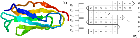
Figure 39: (a) NS conformation of DDFLN4 taken from the PDB (PDB ID: 1ksr). There are seven $\beta$-strands: A (6-9), B (22-28), C (43-48), D (57-59), E (64-69), F (75-83), and G (94-97). In the NS there are 15, 39, 23, 10, 27, 49, and 20 native contacts formed by strands A, B, C, D, E, F, and G with the rest of the protein, respectively. The end-to-end distance in the NS $R_{NS}=40.2$ Å. (b) There are 7 pairs of strands, which have the nonzero number of mutual native contacts in the NS. These pairs are P${}_{\textrm{AB}}$, P${}_{\textrm{AF}}$, P${}_{\textrm{BE}}$, P${}_{\textrm{CD}}$, P${}_{\textrm{CF}}$, P${}_{\textrm{DE}}$, and P${}_{\textrm{FG}}$. The number of native contacts between them are 11, 1, 13, 2, 16, 8, and 11, respectively.

The native conformation of DDFLN4, which has seven $\beta$-strands, enumerated as A to G, was taken from the PDB (PI: 1KSR, Fig. 39a). We assume that residues $i$ and $j$ are in native contact if the distance between them in the native conformation, is shorter than a cutoff distance $d_{c}=6.5$ Å. With this choice of $d_{c}$, the molecule has 163 native contacts. Native contacts exist between seven pairs of $\beta$-strands P${}_{\textrm{AB}}$, P${}_{\textrm{AF}}$, P${}_{\textrm{BE}}$, P${}_{\textrm{CD}}$, P${}_{\textrm{CF}}$, P${}_{\textrm{DE}}$, and P${}_{\textrm{FG}}$ (Fig. 39b).

We used the C_α-Go model Clementi_JMB00 for a molecule. The corresponding parameters of this model are chosen as in Chapter 4. The simulations were carried out in the over-damped limit with the water viscosity $\zeta=50\frac{m}{\tau_{L}}$ The Brownian dynamics equation (Eq. 19) was numerically solved by the simple Euler method (Eq. 20). Due to the large viscosity, we can choose a large time step $\Delta t=0.1\tau_{L}$, and this choice allows us to study unfolding at low loading rates. In the constant velocity force simulations, we follow the protocol described in section 3.1.2. The mechanical unfolding sequencing was studied by monitoring the fraction of native contacts of the $\beta$-strands and of their seven pairs as a function of $\Delta R$, which is admitted a good reaction coordinate.

9.3 Results

9.3.1 Robustness of peak at end-to-end extension $\Delta R\approx 1.5$ nm and absence of maximum at $\Delta R\approx 22$ nm at low pulling speeds

Figure 40: (a) Typical force-extension curves for $v=7.2\times 10^{6}$ nm/s. (b) The same as in (a) but for $v=6.4\times 10^{5}$ nm/s. (c) The same as in (a) but for $v=5.8\times 10^{4}$ nm/s. The arrow roughly refers to locations of additional peaks for two trajectories (red and green). (d) The same as in (c) but for $v=2.6\times 10^{4}$ mn/s.

In the previous high pulling speed ($v=3.6\times 10^{7}$ nm/s) Go simulations MSLi_JCP08 , the force-extension curve shows two peaks at $\Delta R\approx 1.5$ nm and 10 nm, while the experiments showed that peaks appear at $\Delta R\approx 12$ nm and 22 nm. The question we ask if one can reproduce the experimental results at low pulling speeds. Within our computational facilities, we were able to perform simulations at the lowest $v=2.6\times 10^{4}$ nm/s which is about three orders of magnitude lower than that used before MSLi_JCP08 .

Fig. 40 show force-extension curves for four representative pulling speeds. For the highest $v=7.2\times 10^{6}$ nm/s (Fig. 40a), there are two peaks located at extensions $\Delta R\approx 1.5$ nm and 9 nm. As evident from Figs. 40b, c and d, the existence of the first peak remains robust against reduction of $v$. Positions of $f_{max1}$ weakly fluctuate over the range $0.9\lesssim\Delta R\lesssim 1.8$ nm for all values of $v$ (Fig. 41). As $v$ is reduced, $f_{max1}$ decreases but this peak does not vanish if one interpolates our results to the lowest pulling speed $v_{exp}=200$ nm/s used in the experiments Schwaiger_NSMB04 (see below).

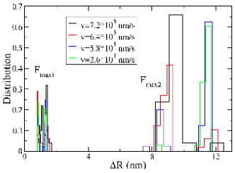
Figure 41: Distributions of positions of $f_{max1}$ and $f_{max2}$ for $v=7.2\times 10^{6}$ (black), $6.4\times 10^{5}$ (red) , $5.8\times 10^{4}$ (blue) and 2.6$\times 10^{4}$ mn/s (green.

Thus, opposed to the experiments, the first peak occurs already at small end-to-end extensions. We do not exclude a possibility that such a peak was overlooked by experiments, as it happened with the titin domain I27. Recall that, for this domain the first AFM experiment Rief_Science97 did not trace the hump which was observed in the later simulations Lu_BJ98 and experiments Marszalek_Nature99 .

Positions of the second peak $f_{max2}$ are more scattered compared to $f_{max1}$, ranging from about 8 nm to 12 nm (Fig. 41). Overall, they move toward higher values upon reduction of $v$ (Fig. 40). If at $v=6.4\times 10^{5}$ nm/s only about 15$\%$ trajectories display $\Delta R_{max2}>10$ nm, then this percentage reaches 65$\%$ and 97% for $v=5.8\times 10^{4}$ nm/s and $2.6\times 10^{4}$ nm/s, respectively (Fig. 41).

At low $v$, unfolding pathways show rich diversity. For $v\gtrsim 6.4\times 10^{5}$ nm/s, the force-extension profile shows only two peaks in all trajectories studied (Fig. 40a and 40b),while for lower speeds $v=5.8\times 10^{4}$ nm/s and $2.6\times 10^{4}$ nm/s, about $4\%$ trajectories display even four peaks (Fig. 40c and 40d), i.e. the four-state behavior.

We do not observe any peak at $\Delta R\approx 22$ nm for all loading rates (Fig. 40), and it is very unlikely that it will appear at lower values of $v$. Thus, the Go model, in which non-native interactions are neglected, fails to reproduce this experimental observation. Whether inclusion of non-native interactions would cure this problem requires further studies.

9.3.2 Dependence of mechanical pathways on loading rates

The considerable fluctuations of peak positions and occurrence of even three peaks already suggest that unfolding pathways, which are kinetic in nature, may change if $v$ is varied. To clarify this point in more detail, we show $\Delta R$-dependencies of native contacts of all $\beta$-strands and their pairs for $v=7.2\times 10^{6}$ nm/s (Figs. 42a,b) and $v=2.6\times 10^{4}$ nm/s (Figs. 42c,d). For $v=7.2\times 10^{6}$ nm/s, one has the following unfolding pathways:

$$G\rightarrow F\rightarrow(C,E,D)\rightarrow B\rightarrow A,$$ (60a)

$$P_{AF}\rightarrow P_{BE}\rightarrow(P_{FG},P_{CF})\rightarrow P_{CD}\rightarrow P_{DE}\rightarrow P_{AB}.$$ (60b)

According to this scenario, the unfolding initiates from the C-terminal, while the experiments Schwaiger_NSMB04 showed that strands A and B unfold first. For $v=2.6\times 10^{4}$ nm/s, Fig. 42c gives the following sequencing

$$(A,B)\rightarrow(C,D,E)\rightarrow(F,G),$$ (61a)

$$P_{AF}\rightarrow(P_{BE},P_{AB})\rightarrow P_{CF}\rightarrow(P_{CD},P_{DE},P_{FG}).$$ (61b)

Figure 42: (a) Dependences of averaged fractions of native contacts formed by seven strands on $\Delta R$ for $v=7.2\times 10^{6}$ nm/s. (b) The same as in (a) but for pairs of strands. (c)-(d) The same as in a)-b) but for $v=2.6\times 10^{4}$ nm/s. Results were averaged over 50 trajectories.

We obtain the very interesting result that at this low loading rate, in agreement with the AFM experiments Schwaiger_NSMB04 , the N-terminal detaches from a protein first. For both values of $v$, the first peak corresponds to breaking of native contacts between strands A and F (Fig. 42d and Fig. 42b). However, the structure of unfolding intermediates, which correspond to this peak, depends on $v$. For $v=7.2\times 10^{6}$ nm/s (Fig. 42a,b), at $\Delta R\approx 1.5$ nm, native contacts between F and G are broken and strand G has already been unstructured (Fig. 42a). Therefore, for this pulling speed, the intermediate consists of six ordered strands A-F (see Fig. 43a for a typical snapshot). In the $v=2.6\times 10^{4}$ nm/s case, just after the first peak, none of strands unfolds completely (Fig. 42c), although (A,F) and (B,E) contacts have been already broken (Fig. 42d). Thus, the intermediate looks very different from the high $v$ case, as it has all secondary structures partially structured (see (Fig. 43b) for a typical snapshot). Since the experiments Schwaiger_NSMB04 showed that intermediate structures contain five ordered strands C-G, intermediates predicted by simulations are more ordered than the experimental ones. Even though, our low loading rate Go simulations provide the same pathways as on the experiments. The difference between theory and experiments in intermediate structures comes from different locations of the first peak. It remains unclear if this is a shortcoming of Go models or of the experiments because it is hard to imagine that a $\beta$-protein like DDFLN4 displays the first peak at such a large extension $\Delta R\approx 12$ nm Schwaiger_NSMB04 . The force-extension curve of the titin domain I27, which has a similar native topology, for example, displays the first peak at $\Delta R\approx 0.8$ nm Marszalek_Nature99 . From this prospect, the theoretical result is more favorable.

Figure 43: (a) Typical snapshot obtained at $\Delta R=2$ nm and $v=7.2\times 10^{6}$ nm/s. A single contact between strand A (blue spheres) and strand F (orange) was broken. Native contacts between F and G (red) are also broken and G completely unfolds. (b) The same as in (a) but for $v=2.6\times 10^{4}$ nm/s. Native contacts between A and F and between B and E are broken but all strands are remain partially structured. (c) Typical snapshot obtained at $\Delta R=11$ nm and $v=7.2\times 10^{6}$ nm/s. Native contacts between pairs are broken except those between strands A and B. All 11 unbroken contacts are marked by solid lines. Strands A and B do not unfold yet. (d) The same as in (c) but for $v=2.6\times 10^{4}$ nm/s. Two from 11 native contacts between F and G are broken (dashed lines). Contacts between other pairs are already broken, but F and G remain structured.

The strong dependence of unfolding pathways on loading rates is also clearly seen from structures around the second peak. In the $v=7.2\times 10^{6}$ nm/s case, at $\Delta R\approx 11$ nm, strands A and B remain structured, while other strands detach from a protein core (Fig. 42a and Fig. 43c). This is entirely different from the low loading case, where A and B completely unfold but F and G still survive (Fig. 42c and Fig. 43d). The result, obtained for $v=2.6\times 10^{4}$ nm/s, is in full agreement with the experiments Schwaiger_NSMB04 that at $\Delta R\approx 12$ nm, A and B detached from the core.

Note that the unfolding pathways given by Eq. (60a), 60b, 61a, and 61b are valid in the statistical sense. In all 50 trajectories studied for $v=7.2\times 10^{5}$ nm/s, strands A and B always unfold last, and F and G unfold first (Eq. 60a), while the sequencing of unfolding events for C, D and E depends on individual trajectories. At $v=2.6\times 10^{4}$ nm/s, most of trajectories follow the pathway given by Eq. (61a), but we have observed a few unusual pathways, as it is illustrated in Fig. 44. Having three peaks in the force-extension profile, the evolution of native contacts of F and G display an atypical behavior. At $\Delta R\approx 7$ nm, these strands fully unfold (Fig. 44c), but they refold again at $\Delta R\approx 11$ nm (Fig. 44b and 44d). Their final unfolding takes place around $\Delta R\approx 16.5$ nm. As follows from Fig. 44b, the first peak in Fig. 44a corresponds to unfolding of G. Strands A and B unfold after passing the second peak, while the third maximum occurs due to unfolding of C-G , i.e. of a core part shown in Fig. 44d.

Figure 44: (a) Force-extension curve for an atypical unfolding pathway at $v=2.6\times 10^{4}$ nm/s. (b) Dependence of fractions of native contacts of seven strands on $\Delta R$. Snapshot at $\Delta R=7.4$ nm (c) and $\Delta R=11$ nm (d).

The dependence of unfolding pathways on $v$ is understandable. If a protein is pulled very fast, the perturbation, caused by the external force, does not have enough time to propagate to the fixed N-terminal before the C-terminal unfolds. Therefore, at very high $v$, we have the pathway given by Eq. (60a). In the opposite limit, it does matter what end is pulled as the external force is uniformly felt along a chain. Then, a strand, which has a weaker link with the core, would unfold first.

9.3.3 Computation of free energy landscape parameters

As mentioned above, at low loading rates, for some trajectories, the force-extension curve does not show two, but three peaks. However, the percentage of such trajectories is rather small, we will neglect them and consider DDFLN4 as a three-state protein. Recently, using dependencies of unfolding times on the constant external force and the non-linear kinetic theory Dudko_PRL06 , we obtained distances $x_{u1}\approx x_{u2}\approx 13\AA$ MSLi_JCP08 . These values seem to be large for $\beta$-proteins like DDFLN4, which are supposed to have smaller $x_{u}$ compared to $\alpha/\beta$- and $\alpha$-ones MSLi_BJ07a . A clear difference between theory and experiments was also observed for the unfolding barrier $\Delta G^{\ddagger}_{1}$. In order to see if one can improve our previous results, we will extract the FEL parameters by a different approach. Namely, assuming that all FEL parameters of the three-state DDFLN4, including the barrier between the second TS and the IS $\Delta G^{\ddagger}_{2}$ (see Ref. MSLi_JCP08, for the definition), can be determined from dependencies of $f_{max1}$ and $f_{max2}$ on $v$, we calculate them in the the Bell-Evans-Rirchie (BER) approximation as well as beyond this approximation.

Estimation of $x_{u1}$ and $x_{u2}$ in the BER approximation

In this approximation, $x_{u1}$ and $x_{u2}$ are related to $v$, $f_{max1}$ and $f_{max2}$ by the following equation Evans_BJ97 :

$$f_{maxi}\;=\;\frac{k_{B}T}{x_{ui}}\ln\left[\frac{vx_{ui}}{k_{ui}(0)k_{B}T}\right],i=1,2,$$ (62)

where $k_{ui}(0)$ is unfolding rates at zero external force. In the low force regime ($v\lesssim 2\times 10^{6}$ nm/s), the dependence of $f_{max}$ on $v$ is logarithmic and $x_{u1}$ and $x_{u2}$ are defined by slopes of linear fits in Fig. 45. Their values are listed in Table 6. The estimate of $x_{u2}$ agrees very well with the experimental Schwaiger_EMBO05 as well as with the previous theoretical result MSLi_JCP08 . The present value of $x_{u1}$ agrees with the experiments better than the old one MSLi_JCP08 . Presumably, this is because it has been estimated by the same procedure as in the experiments Schwaiger_EMBO05 .

It is important to note that the logarithmic behavior is observed only at low enough $v$. At high loading rates, the dependence of $f_{max}$ on $v$ becomes power-law. This explains why all-atom simulations, performed at $v\sim 10^{9}$ nm/s for most of proteins, are not able to provide reasonable estimations for $x_{u}$.

The another interesting question is if the peak at $\Delta R\approx 1.5$ nm disappears at loading rates used in the experiments Schwaiger_EMBO05 . Assuming that the logarithmic dependence in Fig. 45 has the same slope at low $v$, we interpolate our results to $v_{exp}=200$ nm/s and obtain $f_{max1}(v_{exp})\approx 40$ pN. Thus, in the framework of the Go model, the existence of the first peak is robust at experimental speeds.

Figure 45: Dependences of $F_{max1}$ (open circles) and $F_{max2}$ (open squares) on $v$. Results were obtained by using the Go model. Straight lines are fits to the BER equation ($y=-20.33+11.424ln(x)$ and $y=11.54+6.528ln(x)$ for $F_{max1}$ and $F_{max2}$, respectively). Here $f_{max}$ and $v$ are measured in pN and nm/s, respectively. From these fits we obtain $x_{u1}=3.2\AA\,$ and $x_{u2}=5.5\AA$. The solid circle and triangle correspond to $f_{max1}\approx 40$ pN and $f_{max2}\approx 46$ pN, obtained by interpolation of linear fits to the experimental value $v=200$ nm/s. Fitting to the nonlinear microscopic theory (dashed lines) gives $x_{u1}=7.0\AA\,\Delta G^{\ddagger}_{1}=19.9k_{B}T,x_{u2}=9.7\AA\,$, and $\Delta G^{\ddagger}_{2}=20.9k_{B}T$.

Beyond the BER approximation

In the BER approximation, one assumes that the location of the TS does not move under the action of an external force. Beyond this approximation, $x_{u}$ and unfolding barriers can be extracted, using the following formula Dudko_PRL06 :

$$f_{max}\,=\frac{\Delta G^{\ddagger}}{\nu x_{u}}\left\{1-\left[\frac{k_{B}T}{\Delta G^{\ddagger}}\textrm{ln}\frac{k_{B}Tk_{u}(0)e^{\Delta G^{\ddagger}/k_{B}T+\gamma}}{x_{u}v}\right]^{\nu}\right\}$$ (63)

Here, $\Delta G^{\ddagger}$ is the unfolding barrier, $\nu=1/2$ and 2/3 for the cusp Hummer_BJ03 and the linear-cubic free energy surface Dudko_PNAS03 , respectively. $\gamma\approx 0.577$ is the Euler-Mascheroni constant. Note that $\nu=1$ corresponds to the phenomenological BER theory (Eq. 62). If $\nu\neq 1$, then Eq. (63) can be used to estimate not only $x_{u}$, but also $\Delta G^{\ddagger}$. Since the fitting with $\nu=1/2$ is valid in a wider force interval compared to the $\nu=2/3$ case, we consider the former case only. The region, where the $\nu=1/2$ fit works well, is expectantly wider than that for the Bell scenario (Fig. 45). From the nonlinear fitting (Eq. 63), we obtain $x_{u1}=7.0\AA\,$, and $x_{u2}=9.7\AA\,$ which are about twice as large as the Bell estimates (Table 6). Using AFM data, Schlierf and Rief Schlierf_BJ06 , have shown that beyond BER approximation $x_{u}\approx 11\AA\,$. This value is close to our estimate for $x_{u2}$. However, a full comparison with experiments is not possible as these authors did not consider $x_{u1}$ and $x_{u2}$ separately. The present estimations of these quantities are clearly lower than the previous one MSLi_JCP08 (Table 6). The lower values of $x_{u}$ would be more favorable because they are expected to be not high for beta-rich proteins MSLi_BJ07a like DDFLN4. Thus, beyond BER approximation, the method based on Eq. (63) provides more reasonable estimations for $x_{ui}$ compared to the method, where these parameters are extracted from unfolding rates MSLi_JCP08 . However, in order to decide what method is better, more experimental studies are required.

The corresponding values for $\Delta G^{\ddagger}_{1}$, and $\Delta G^{\ddagger}_{2}$ are listed in Table 6. The experimental and previous theoretical results MSLi_JCP08 are also shown for comparison. The present estimates for both barriers agree with the experimental data, while the previous theoretical value of $\Delta G^{\ddagger}_{1}$ fits to experiments worse than the current one.

	BER approximation		Beyond BER approximation
	$x_{u1}(\AA)$	$x_{u2}(\AA)$	$x_{u1}(\AA)$	$x_{u2}(\AA)$	$\Delta G^{\ddagger}_{1}/k_{B}T\;$	$\Delta G^{\ddagger}_{2}/k_{B}T\;$
Theory MSLi_JCP08	6.3 $\pm$ 0.2	5.1 $\pm$ 0.2	13.1	12.6	25.8	18.7
Theory (this work)	3.2 $\pm$ 0.2	5.5 $\pm$ 0.2	7.0	9.7	19.9	20.9
Exp. Schwaiger_EMBO05 ; Schlierf_BJ06	4.0 $\pm 0.4$	5.3 $\pm$ 0.4			17.4	17.2

Table 6: Parameters $x_{u1}$, and $x_{u2}$ were obtained in the Bell and beyond-Bell approximation. Theoretical values of the unfolding barriers were extracted from the microscopic theory of Dudko et al (Eq. 28) with $\nu=1/2$. The experimental estimates were taken from Ref. MSLi_JCP08, .

9.3.4 Thermal unfolding pathways

In order to see if the thermal unfolding pathways are different from the mechanical ones, we performed zero-force simulations at $T=410$ K. The progress variable $\delta$ is used as a reaction coordinate to monitor pathways (see Chapter 3). From Fig. 46, we have the following sequencing for strands and their pairs:

$$G\rightarrow(B,C,E)\rightarrow(A,F,D),$$ (64a)

$$P_{AF}\rightarrow P_{BE}\rightarrow(P_{CD},P_{CF})\rightarrow(P{AB},P_{FG},P_{DE}).$$ (64b)

It should be noted that these pathways are just major ones as other pathways are also possible. The pathway given by Eq. (64b), e.g., occurs in 35% of events. About 20% of trajectories follow $P_{AF}\rightarrow P_{CF}\rightarrow P_{BE}\rightarrow(P_{CD},P{AB},P_{FG},P_{DE})$ scenario. We have also observed the sequencing $P_{AF}\rightarrow P_{BE}\rightarrow(P_{CF},P{AB},P_{FG},P_{DE})\rightarrow P_{CD}$, and $P_{BE}\rightarrow P_{AF}\rightarrow(P_{CD},P{CF},P_{AB},P_{FG},P_{DE})$ in 12% and 10% of runs, respectively. Thus, due to strong thermal fluctuations, thermal unfolding pathways are more diverse compared to mechanical ones. From Eqs. 60a, 60b, 61a, 61b, 64a, and 64b, it is clear that thermal unfolding pathways of DDFLN4 are different from the mechanical pathways. This is also illustrated in Fig. 46c. As in the mechanical case (Fig. 43a and 43b), the contact between A and F is broken, but the molecule is much less compact at the same end-to-end distance. Although 7 contacts ($\approx 64$%) between strands F and G remain survive, all contacts of pairs $P_{AF},P_{BE}$ and $P_{CD}$ are already broken.

Figure 46: Thermal unfolding pathways. (a) Dependence of native contact fractions of seven strands on the progress variable $\delta$ at $T=410$ K. (b) The same as in (a) but for seven strand pairs. (c) A typical snapshot at $\Delta R\approx 1.8$ nm. The contact between strands S1 and S6 is broken but 7 contacts between strands S6 and S7 (solid lines) still survive.

The difference between mechanical and thermal unfolding pathways is attributed to the fact that thermal fluctuations have a global effect on the biomolecule, while the force acts only on its termini. Such a difference was also observed for other proteins like I27 Paci_PNAS00 and Ub MSLi_BJ07 ; Mitternacht_Proteins06 . We have also studied folding pathways of DDFLN4 at $T=285$ K. It turns out that they are reverse of the thermal unfolding pathways given by Eqs. 64a and 64b. It would be interesting to test our prediction on thermal folding/unfolding of this domain experimentally.

9.4 Conclusions

The key result of this chapter is that mechanical unfolding pathways of DDFLN4 depend on loading rates. At large $v$ the C-terminal unfolds first, but the N-terminal unfolds at low $v\sim 10^{4}$ nm/s. The agreement with the experiments Schwaiger_NSMB04 is obtained only in low loading rate simulations. The dependence of mechanical unfolding pathways on the loading rates was also observed for I27 (M.S. Li, unpublished). On the other hand, the previous studies Irback_PNAS05 ; MSLi_BJ07 showed that mechanical unfolding pathways of the two-state Ub do not depend on the force strength. Since DDFLN4 and I27 are three-state proteins, one may think that the unfolding pathway change with variation of the pulling speed, is universal for proteins that unfold via intermediates. A more comprehensive study is needed to verify this interesting issue.

Dependencies of unfolding forces on pulling speeds have been widely used to probe FEL of two-state proteins Best_PNAS02 . However, to our best knowledge, here we have made a first attempt to apply this approach to extract not only $x_{ui}$, but also $\Delta G^{\ddagger}_{i}$ ($i=1,$ and 2) for a three-state protein. This allows us to improve our previous results MSLi_JCP08 . More importantly, a better agreement with the experimental data Schwaiger_EMBO05 ; Schlierf_BJ06 suggests that this method is also applicable to other multi-state biomolecules. Our study clearly shows that the low loading rate regime, where FEL parameters can be estimated, occurs at $v\leq 10^{6}$ nm/s which are about two-three orders of magnitude lower than those used in all-atom simulations. Therefore, at present, deciphering unfolding FEL of long proteins by all-atom simulations with explicit water is computationally prohibited. From this prospect, coarse-grained models are of great help.

We predict the existence of a peak at $\Delta R\sim 1.5$ nm even at pulling speeds used in now a day experimental setups. This result would stimulate new experiments on mechanical properties of DDFLN4. Capturing the experimentally observed peak at $\Delta R\sim 22$ nm remains a challenge to theory.

Chapter 10 Protein mechanical unfolding: importance of non-native interactions

10.1 Introduction

In this chapter, we continue to study the mechanical unfolding of DDFLN4 using the all-atom simulations. Motivation for this is that Go model can not explain some experimental results. Namely, in the AFM force-extension curve (Schwaiger et al. Schwaiger_NSMB04 ; Schwaiger_EMBO05 observed two peaks at $\Delta R\approx 12$ and 22 nm. However, using a Go model Clementi_JMB00 , Li et al.MSLi_JCP08 and Kouza and Li (chapter 9) have also obtained two peaks but they are located at $\Delta R\approx 1.5$ and 11 nm. A natural question to ask is if the disagreement between experiments and theory is due to over-simplification of the Go modeling, where non-native interactions between residues are omitted. In order to answer this question, we have performed all-atom MD simulations, using the GROMOS96 force field 43a1 Gunstren_96 and the SPC explicit water solvent Berendsen81 .

We have shown that, two peaks do appear at almost the same positions as in the experiments Schwaiger_NSMB04 ; Schwaiger_EMBO05 and more importantly, the peak at $\Delta R\approx 22$ nm comes from the non-native interactions. It explains why it has not been seen in the previous Go simulationsMSLi_JCP08 . In our opinion, this result is very important as it opposes to the common belief West_BJ06 ; MSLi_BJ07a that mechanical unfolding properties are governed by the native topology. In addition to two peaks at large $\Delta R$, in agreement with the Go results MSLi_JCP08 , we have also observed a maximum at $\Delta R\approx 2$ nm. Because such a peak was not detected by the AFM experiments Schwaiger_NSMB04 ; Schwaiger_EMBO05 , further experimental and theoretical studies are required to clarify this point.

The results of this chapter are adapted from Ref. Kouza_JCP09 .

10.2 Materials and Methods

We used the GROMOS96 force field 43a1 Gunstren_96 to model DDFLN4 which has 100 amino acids, and the SPC water model Berendsen81 to describe the solvent (see also chapter 4). The Gromacs version 3.3.1 has been employed. The protein was placed in an cubic box with the edges of 4.0, 4.5 and 43 nm, and with 76000 - 78000 water molecules (Fig. 47).

Figure 47: The solvated system in the orthorhombic box of water (cyan). VMD software VMD was used for a plot.

In all simulations, the GROMACS program suite Berendsen_CPC95 ; Lindahl01 was employed. The equations of motion were integrated by using a leap-frog algorithm with a time step of 2 fs. The LINCS Hess_JCC97 was used to constrain bond lengths with a relative geometric tolerance of $10^{-4}$. We used the particle-mesh Ewald method to treat the long-range electrostatic interactions Darden93 . The nonbonded interaction pair-list were updated every 10 fs, using a cutoff of 1.2 nm.

The protein was minimized using the steepest decent method. Subsequently, unconstrained MD simulation was performed to equilibrate the solvated system for 100 ps at constant pressure (1 atm) and temperature $T=300$ K with the help of the Berendsen coupling procedure Berendsen84 . The system was then equilibrated further at constant temperature $T$ = 300 K and constant volume. Afterward, the N-terminal was kept fixed and the force was applied to the C-terminal through a virtual cantilever moving at the constant velocity $v$ along the biggest $z$-axis of simulation box. During the simulations, the spring constant was chosen as $k=1000kJ/(mol\times nm^{2})\approx 1700$ pN/nm which is an upper limit for $k$ of a cantilever used in AFM experiments. Movement of the pulled termini causes an extension of the protein and the total force can be measured by $F=kvt$. The resulting force is computed for each time step to generate a force extension profile, which has peaks showing the most mechanically stable places in a protein.

Overall, the simulation procedure is similar to the experimental one, except that pulling speeds in our simulations are several orders of magnitude higher than those used in experiments. We have performed simulations for $v=10^{6},5\times 10^{6},1.2\times 10^{7}$, and $2.5\times 10^{7}$ nm/s, while in the AFM experiments one took $v\sim 100-1000$ nm/s Schwaiger_NSMB04 . For each value of $v$ we have generated 4 trajectories.

A backbone contact between amino acids $i$ and $j$ ($|i-j|>3$) is defined as formed if the distance between two corresponding C_α-atoms is smaller than a cutoff distance $d_{c}=6.5$ Å. With this choice, the molecule has 163 native contacts. A hydrogen bond is formed provided the distance between donor D (or atom N) and acceptor A (or atom O) $\leq 3.5\AA\,$ and the angle D-H-A $\geq 145^{\circ}$.

The unfolding process was studied by monitoring the dependence of numbers of backbone contacts and HBs formed by seven $\beta$-strands enumerated as A to G (Fig. 39a) on the end-to-end extension. In the NS, backbone contacts exist between seven pairs of $\beta$-strands P${}_{\textrm{AB}}$, P${}_{\textrm{AF}}$, P${}_{\textrm{BE}}$, P${}_{\textrm{CD}}$, P${}_{\textrm{CF}}$, P${}_{\textrm{DE}}$, and P${}_{\textrm{FG}}$ as shown in Fig. 39b. Additional information on unfolding pathways was also obtained from the evolution of numbers of contacts of these pairs.

10.3 Results

10.3.1 Existence of three peaks in force-extension profile

Since the results obtained for four pulling speeds (Material and Methods) are qualitatively similar, we will focus on the smallest $v=10^{6}$ nm/s case. The force extension curve, obtained at this speed, for the trajectory 1, can be divided into four regions (Fig. 48):

Figure 48: Force-extension profile for trajectory 1 for $v=10^{6}$ nm/s. Vertical dashed lines separate four unfolding regimes. Shown are typical snapshots around three peaks. Heights of peaks (from left) are $f_{max1}=695$ pN, $f_{max2}=704$ pN, and $f_{max3}=626$ pN.

Region I ($0\lesssim\Delta R\lesssim 2.42$ nm). Due to thermal fluctuations, the total force fluctuates a lot, but, in general, it increases and reaches the first maximum $f_{max1}=695$ pN at $\Delta R$ 2.42 nm. A typical snapshot before the first unfolding event (Fig. 48) shows that structures remain native-like. During the first period, the N-terminal part is being extended, but the protein maintains all $\beta$-sheet secondary structures (Fig. 49b). Although, the unfolding starts from the N-terminal (Fig. 49b), after the first peak, strand G from the C-termini got unfolded first (Fig. 49c and 49f). In order to understand the nature of this peak on the molecular level, we consider the evolution of HBs in detail. As a molecule departs from the NS, non-native HBs are created and at $\Delta R=2.1$ nm, e.g., a non-native $\beta$-strand between amino acids 87 and 92 (Fig. 49b) is formed. This leads to increase of the number of HBs between F and G from 4 (Fig. 49d) to 9 (Fig. 49e). Structures with the enhanced number of HBs should show strong resistance to the external perturbation and the first peak occurs due to their unfolding (Fig. 49b). It should be noted that this maximum was observed in the Go simulations MSLi_JCP08 ; MSLi_JCP09 , but not in the experiments Schwaiger_NSMB04 ; Schwaiger_EMBO05 . Both all-atom and Go simulations reveal that the unfolding of G strand is responsible for its occurrence.

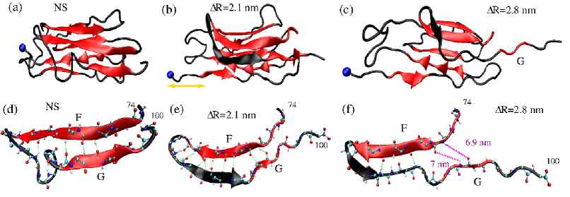
Figure 49: (a) The NS conformation is shown for comparison with the other ones. (b) A typical conformation before the first unfolding event takes place ($\Delta R\approx$ 2.1 nm). The yellow arrow shows a part of protein which starts to unfold. An additional non-native $\beta$-strand between amino acids 87 and 92 is marked by black color. (c) A conformation after the first peak, at $\Delta R\approx$ 2.8 nm, where strand G has already detached from the core. (d) The same as in (a) but 4 HBs (green color) between $\beta$-strands are displayed. (e) The same as in (b) but all 9 HBs are shown. (f) The same as in (c) but broken HBs (purple) between F and G are displayed.

Region II ($2.42nm\lesssim\Delta R\lesssim 13.36$ nm): After the first peak, the force drops rapidly from 695 to 300 pN and secondary structure elements begin to break down. During this period, strands A, F and G unfold completely, whereas B, C, D and E strands remain structured (see Fig. 48 for a typical snapshot).

Region III ($13.36nm\lesssim\Delta R\lesssim 22.1$ nm: During the second and third stages, the complete unfolding of strands D and E takes place. Strands B and C undergo significant conformational changes, losing their equilibrium HBs. Even though a core formed by these strands remains compact (see bottom of Fig. 48 for a typical snapshot). Below we will show in detail that the third peak is associated with breaking of non-native HBs between strands B and C.

Region IV ($\Delta R\gtrsim 22.1$ nm: After breaking of non-native HBs between B and C, the polypeptide chain gradually reaches its rod state.

The existence of three pronounced peaks is robust as they are observed in all four studied trajectories (similar results obtained in other three runs are not shown). It is also clearly evident from Fig. 50, which displays the force-extension curve averaged over 4 trajectories.

Figure 50: The averaged over 4 trajectories force-extension profile. $v=10^{6}$ nm/s.

10.3.2 Importance of non-native interactions

As mentioned above, the third peak at $\Delta R\approx 22$ nm was observed in the experiments but not in Go models MSLi_JCP08 ; MSLi_JCP09 , where non-native interactions are omitted. In this section, we show, at molecular level, that these very interactions lead to its existence. To this end, we plot the dependence of the number of native contacts formed by seven strands and their pairs on $\Delta R$. The first peak corresponds to unfolding of strand G (Fig. 51a) as all (A,F) and (F,G) contacts are broken just after passing it (Fig. 51b). Thus, the structure of the first IS1, which corresponds to this peak, consists of 6 ordered strands A-F (see Fig. 49c for a typical snapshot).

The second unfolding event is associated with full unfolding of A and F and drastic decrease of native contacts of B and C (Fig. 51a. After the second peak only (B,E), (C,D) and (D,E) native contacts survive (51b). The structure of the second intermediate state (IS2) contains partially structured strands B, C, D and E. A typical snapshot is displayed in top of Fig. 48.

Remarkably, for $\Delta R\gtrsim 17$ nm, none of native contacts exists, except very small fluctuation of a few contacts of strand B around $\Delta R\approx 22.5$ nm (Fig. 51a). Such a fluctuation is negligible as it is not even manifested in existence of native contacts between corresponding pairs (A,B) and (B,E) (Fig. 51b). Therefore, we come to a very interesting conclusion that the third peak centered at $\Delta R\approx 22.5$ nm is not related to native interactions. This explains why it was not detected by simulations MSLi_JCP08 ; MSLi_JCP09 using the Go model Clementi_JMB00 .

Figure 51: (a) Dependence of the number of native backbone contacts formed by individual strands on $\Delta R$. Arrows refer to positions of three peaks in the force-extension curve. (b) The same as in (a) but for pairs of strands. (c) The same as in (a) but for all contacts (native and non-native). (d) The same as in (c) but for HBs.

The mechanism underlying occurrence of the third peak may be revealed using the results shown in Fig. 51c, where the number of all backbone contacts (native and non-native) is plotted as a function of $\Delta R$. Since, for $\Delta R\gtrsim 17$ nm, native contacts vanish, this peak is associated with an abrupt decrease of non-native contacts between strands B and C. Its nature may be also understood by monitoring the dependence of HBs on $\Delta R$ (Fig. 51d), which shows that the last maximum is caused by loss of HBs of these strands. More precisely, five HBs between B and C, which were not present in the native conformation, are broken (Fig. 52). Interestingly, these bonds appear at $\Delta R\gtrsim$ 15 nm, i.e. after the second unfolding event (Fig. 52). Thus, our study can not only reproduce the experimentally observed peak at $\Delta R\approx 22$ nm, but also shed light on its nature on the molecular level. From this perspective, all-atom simulations are superior to experiments.

Figure 52: Dependence of the number of HBs between pairs of strands. Red arrow refers to a position where non-native HBs between strands B and C start to appear. Their creation leads to the maximum centered at $\Delta R\approx 22.4$ nm. Upper snapshot shows five HBs between B an C before the third unfolding event. Lower snapshot is a fragment after the third peak, where all HBs are already broken (purple dotted lines).

One corollary from Fig. 51a-d is that one can not provide a complete description of the unfolding process based on the evolution of only native contacts. It is because, as a molecule extends, its secondary structures change and new non-native secondary structures may occur. Beyond the extension of 17-18 nm (see snapshot at bottom of Fig. 48), e.g., the protein lost all native contacts, but it does not get a extended state without any structures. Therefore, a full description of mechanical unfolding may be obtained by monitoring either all backbone contacts or HBs, as these two quantities give the same unfolding picture (Fig. 51c and 51d).

10.3.3 Unfolding pathways

Figure 53: The $\Delta R$ dependence of the number of HBs, formed by seven strands, for trajectory 2, 3 and 4. $v=10^{6}$ nm/s.

To obtain sequencing of unfolding events, we use dependencies of the number of HBs on $\Delta R$. From Fig. 51d and Fig. 53, we have the following unfolding pathways for four trajectories:

$$G\rightarrow F\rightarrow A\rightarrow(D,E)\rightarrow(B,C),\;\;\textrm{Trajectory 1},$$

$$G\rightarrow F\rightarrow A\rightarrow B\rightarrow C\rightarrow(D,E),\;\;\textrm{Trajectory 2},$$

$$G\rightarrow F\rightarrow A\rightarrow E\rightarrow B\rightarrow D\rightarrow C,\;\;\textrm{Trajectory 3}$$

$$G\rightarrow F\rightarrow A\rightarrow(D,E)\rightarrow C\rightarrow B,\;\;\textrm{Trajectory 4}.$$ (65)

Although four pathways, given by Eq. (65) are different, they share a common feature that the C-terminal unfolds first. This is consistent with the results obtained by Go simulations at high pulling speeds $v\sim 10^{6}$ nm/s MSLi_JCP08 , but contradicts to the experiments Schwaiger_NSMB04 ; Schwaiger_EMBO05 , which showed that strands A and B from the N-termini unfold first. On the other hand, our more recent Go simulations MSLi_JCP09 have revealed that the agreement with the experimental results is achieved if one performs simulations at relatively low pulling speeds $v\sim 10^{4}$ nm/s. Therefore, one can expect that the difference in sequencing of unfolding events between present all-atom results and the experimental ones is merely due to large values of $v$ we used. In order to check this, one has to carry out all-atom simulations, at least, at $v\sim 10^{4}$ nm/s, but such a task is far beyond present computational facilities.

10.3.4 Dependence of unfolding forces on the pulling speed

The question we now ask is whether the unfolding FEL of DDFLN4 can be probed by all-atom simulations with explicit water. To this end, we performed simulations at various loading speeds and monitor the dependence of $f_{maxi}(i=1,2,$ and 3) on $v$ (Fig. 54).

Figure 54: Force-extension profiles for four values of $v$ shown next to the curves.

In accordance with theory Evans_BJ97 , heights of three peaks decrease as $v$ is lowered (Fig. 54). Since the force-extension curve displays three peaks, within the framework of all-atom models, the mechanical unfolding of DDFLN4 follows a four-state scenario (Fig. 55a), but not the three-state one as suggested by the experiments Schwaiger_NSMB04 ; Schwaiger_EMBO05 and Go simulations MSLi_JCP08 . The corresponding FEL should have three transition states denoted by TS1, TS2 and TS3. Remember that the first and second peaks in the force-extension profile correspond to IS1 and IS2.

Assuming that the BER theory Bell_Sci78 ; Evans_BJ97 holds for a four-state biomolecule, one can extract the distances $x_{u1}$ (between NS and TS1), $x_{u2}$ (between IS1 and TS2), and $x_{u3}$ (between IS2 and TS3) from Eq. (62). From the linear fits (Fig. 55b), we have $x_{u1}=0.91\AA,x_{u2}=0.17\AA\,,$ and $x_{u3}=0.18\AA$. These values are far below the typical $x_{u}\approx 5\AA\,$, obtained in the experiments Schwaiger_EMBO05 as well as in the Go simulations MSLi_JCP08 ; MSLi_JCP09 . This difference comes from the fact that pulling speeds used in all-atom simulations are to high (Fig. 55). It clearly follows from Eq. (62), which shows that $x_{u}$ depends on what interval of $v$ we use: the larger are values of $f_{max}$, the smaller $x_{u}$. Thus, to obtain $x_{ui}$ close to its experimental counterpart, one has to reduce $v$ by several orders of magnitude and this problem becomes unfeasible. It is also clear why now a day all-atom simulations with explicit water can not be used to reproduce the FEL parameters, obtained from experiments. From this point of view coarse-grained models are of great help MSLi_BJ07a ; MSLi_JCP08 . The kinetic microscopic theory Dudko_PRL06 , which is valid beyond the BER approximation, can be applied to extract unfolding barriers $\Delta G^{\ddagger}_{i}(i=1,2,$ and 3). Their values are not presented as we are far from the interval of pulling speeds used in experiments.

Since the first peak was not observed in the experiments Schwaiger_NSMB04 ; Schwaiger_EMBO05 , a natural question emerges is whether it is an artifact of high pulling speeds used in our simulations. Except data at the highest value of $v$ (Fig. 55b), within error bars three maxima are compatible. Therefore, the peak centered at $\Delta R\approx 2$ nm is expected to remain at experimental loading rates. Schwaiger_NSMB04 . The force-extension curve of the titin domain I27, which has a similar native topology, for example, displays the first peak at $\Delta R\approx 0.8$ nm Marszalek_Nature99 .

Figure 55: (a) Schematic plot for the free energy $G$ as a function of $\Delta R$. $\Delta G^{\ddagger}_{i}(i=1,2,$ and 3) refers to unfolding barriers. The meaning of other notations is given in the text. (b) Dependence of heights of three peaks on $v$. Results are averaged over four trajectories for each value of $v$. Straight lines refer to linear fits by Eq. (62) ($y_{1}=163+44x,y_{2}=-2692+235x$ and $y_{3}=-2630+227x$) through three low-$v$ data points. These fits give $x_{u1}=0.91\AA,x_{u2}=0.17\AA\,$, and $x_{u3}=0.18\AA$.

One of possible reasons of why the experiments did not detect this maximum is related to a strong linker effect as a single DDFLN4 domain is sandwiched between Ig domains I27-30 and domains I31-34 from titin Schwaiger_NSMB04 .

10.4 Conclusions

Using the all-atom simulations, we have reproduced the experimental result on existence of two peaks located at $\Delta R\approx 12$ and 22 nm. Our key result is that the later maximum occurs due to breaking of five non-native HBs between strand B and C. It can not be encountered by the Go models in which non-native interactions are neglected MSLi_JCP08 ; MSLi_JCP09 . Thus, our result points to the importance of these interactions for the mechanical unfolding of DDFLN4. The description of elastic properties of other proteins may be not complete ignoring non-native interactions. This conclusion is valuable as the unfolding by an external force is widely believed to be solely governed by native topology of proteins.

Our all-atom simulation study supports the result obtained by the Go model MSLi_JCP08 ; MSLi_JCP09 that an additional peak occurs at $\Delta R\approx 2$ nm due to unfolding of strand G. However, it was not observed by the AFM experiments of Schwaiger et al Schwaiger_NSMB04 ; Schwaiger_EMBO05 . In order to solve this controversy, one has to carry out not only simulations with other force fields but also additional experiments.

CONCLUSIONS

In this thesis we have obtained the following new results. By collecting experimental data and performing extensive on- and off-lattice coarse-grained simulations, it was found that the scaling exponent for the cooperativity of folding-unfolding transition $\zeta\approx 2.2$. This value is clearly higher than the characteristic for the first order transition value $\zeta=2$. Our result supports the previous conjecture MSLi_PRL04 that the melting point is a tricritical point, where the first and second order transition lines meet. Having used CD technique and Go simulations, we studied the folding of protein domain hbSBD in detail. Its thermodynamic parameters such as $\Delta H_{G},\Delta C_{p},\Delta S_{G}$, and $\Delta G_{S}$ were determined. Both experiments and theory support the two-state behavior of hbSBD.

With the help of the Go modeling, we have constructed the FEL for single and three-domain Ub, and DDFLN4. Our estimations of $x_{u}$, $x_{f}$ and $\Delta G^{{\ddagger}}_{u}$ are in acceptable agreement with the experimental data. The effect of pulling direction on FEL was also studied for single Ub. Pulling at Lys48 and C-termini deforms the unfolding FEL as it increases the distance between the NS and TS. It has been shown that unfolding pathways of Ub depend on what terminal is kept fixed. But it remains unclear if this is a real effect or merely an artifact of high pulling speeds we used in simulations. This problem requires further investigation.

It is commonly believed that protein unfolding is governed by the native topology and non-native interactions play a minor role. However, having performed Gromacs all-atom simulations for DDFLN4, for the first time, we have demonstrated that it may depends on the non-native interactions. Namely, they are responsible for occurrence of a peak located at $\Delta R\approx 22$ nm in the force-extension curve. This peak was not seen in Go models as they take into account only native interactions. In addition, based on the Go as well as all-atom simulations, we predict that an addition peak should appear at $\Delta R\approx 1.5$ nm. Since such a peak was not observed in the experiments, our results are expected to draw attention of experimentalists to this fascinating problem.

Our new force RE method is interesting from the methodological point of view. Its successful application to construction of the $T-f$ phase diagram of the three-domain Ub shows that it might be applied to other biomolecules.

APPENDIX: List of abbreviations and symbols

AFM	Atomic Force Microscopy
BER	Bell-Evans-Rirchie
DS	Denaturated State
TS	Transition State
IS	Intermediate State
NS	Native State
MD	Molecular Dynamics
SMD	Stereed Molecular Dynamics
SMFS	Single Molecular Force Spectroscopy
FEL	Free Energy Landscape
RE	Replica Exchange
CD	Circular Dichroism
DDFLN4	Fourth domain of Dictyostelium discoideum filamin
Ub	Ubiquitin
trimer	three-domain ubiquitin
$\Delta R$	end-to-end extension
$x_{f}$	distance between TS ans DS
$x_{u}$	distance between NS and TS
NBA	native basin of attraction
$T-f$	Temperature-force
HBs	Hydrogen bonds
TDE	Thermal denaturated ensemble
FDE	Force denaturated ensemble

References

- (1) Anfinsen, C. B. (1973) Science 181, 223–230.
- (2) Leopold, P, Montal, M, & Onuchic, J. (1992) Proc Natl Acad Sci USA 89, 8721–8725.
- (3) RL., B. (1994) Nature 369(6477), 183.
- (4) Levinthal, C. (1968) J. Chem. Phys. 65, 44–45.
- (5) Finkelshtein, A. V & Ptitsyn, O. B. (2002) Physics of proteins. (Academic Press, London).
- (6) Li, M. S, Klimov, D. K, & Thirumalai, D. (2004) Phys Rev Lett. 93, 268107–268110.
- (7) Fernandez, J. M & Li, H. (2004) Science 303, 1674–1678.
- (8) Li, M. S, Hu, C. K, Klimov, D. K, & Thirumalai, D. (2006) Proc. Natl. Acad. Sci. USA 103, 93–98.
- (9) Florin, E.-L, Moy, V, & Gaub, H. (1994) Science 264, 415–417.
- (10) Matouschek, A. (2003) Current Opinion in Structural Biology 13, 98–109.
- (11) Brockwell, D. J, Paci, E, Zinober, R, Beddard, G, Olmsted, P, Smith, D, Perham, R, & Radford, S. (2003) Nat. Struct. Biol. 10, 731–737.
- (12) Dietz, H, Berkemeier, F, Bertz, M, & Rief, M. (2006) Proc. Natl. Acad. Sci. USA 103, 12724–12728.
- (13) Schwaiger, I, Kardinal, A, Schleicher, M, Noegel, A, & Rief, M. (2004) Nature Struc. Biol. 11, 81–85.
- (14) Humphrey, W, Dalke, A, & Schulten, K. (1996) Journal of Molecular Graphics 14, 33–38.
- (15) Pauling, L & Corey, R. B. (1951) Proc. Natl. Acad. Sci. USA 37, 235–240.
- (16) Pauling, L & Corey, R. B. (1951) Proc. Natl. Acad. Sci. USA 37, 729–740.
- (17) Kendrew, J. C, Dickerson, R. E, Strandberg, B. E, Hart, R. G, Davies, D. R, Phillips, D. C, & Shore, V. C. (1960) Nature 185, 422–427.
- (18) Bax, A & Tjandra, N. (1997) Journal of Biomolecular NMR 10, 289–292.
- (19) Nolting, B. (2005) Protein Folding Kinetics. (Springer, Berlin).
- (20) Fersht, A. (1998) Structure and Mechanism in Protein Science: A Guide to Enzyme Catalysis and Protein Folding. (W. H. Freeman Company).
- (21) Onuchic, J. N & Wolynes, P. G. (2004) Curr. Opin. Struct. Biol. 14, 70–75.
- (22) Bryngelson, J. D & Wolynes, P. G. (1987) Proc Natl Acad Sci USA 84, 7524–7528.
- (23) Clementi, C, Nymeyer, H, & Onuchic, J. N. (2000) J. Mol. Biol. 298, 937–953.
- (24) Koga, N & Takaga, S. (2001) J. Mol. Biol. 313, 171–180.
- (25) Jin, W, Kambara, O, Sasakawa, H, Tamura, A, & Takada, S. (2003) Structure 11, 581–590.
- (26) Kim, P. S & Baldwin, R. L. (1990) Ann. Rev. Biochem. 59, 631–660.
- (27) Ptitsyn, O. B. (1995) Trends Biochem. Sci. 20, 376–379.
- (28) Wetlaufer, D. (1973) Proc. Natl. Acad. Sci. USA 70, 697–701.
- (29) Shakhnovich, E, Abkevich, V, & Ptitsyn, O. (1996) Nature 379, 96–98.
- (30) Guo, Z & Thirumalai, D. (1997) Fold. Des. 2, 377–391.
- (31) Viguera, A. R & Serrano, M. W. L. (1996) Nature Struct. Biol. 3, 874–880.
- (32) Klimov, D. K & Thirumalai, D. (1998) J. Mol. Biol. 282, 471–492.
- (33) Guo, Z & Thirumalai, D. (1995) Biopolymers 36, 83–103.
- (34) Wolynes, P. G. (1997) Proc. Nat. Acad. Sci., USA 94, 6170–6175.
- (35) Go, N. (1983) Ann. Rev. Biophys. Bioeng. 12, 183–210.
- (36) Thirumalai, D, Klimov, D. K, & Woodson, S. A. (1997) Theor. Chem. Accounts 1, 23–30.
- (37) Thirumalai, D. (1995) J. Phys. I (France) 5, 1457–1467.
- (38) Veitshans, T, Klimov, D. K, & Thirumalai, D. (1997) Folding and Design 2, 1–22.
- (39) Jackson, S. E. (1998) Fold Des. 3, R81–R91.
- (40) Garcia-Mira, M. M, M., S, Fischer, N.and Sanchez-Ruiz, J. M, & Munoz, V. (2002) Science 298, 2191–2195.
- (41) Rief, M, Gautel, M, Oesterhelt, F, Fernandez, J. M, & Gaub, H. E. (1997) Science 276, 1109–1112.
- (42) Tskhovrebova, L, Trinick, K, Sleep, J. A, & Simons, M. (1997) Nature 387, 308–312.
- (43) Bustamante, C, Chemla, Y. R, Forde, N. R, & Izhaky, D. (2004) Annu. Rev. Biochem. 73, 705–748.
- (44) Binnig, G, Quate, C. F, & Berger, C. H. (1986) Phys. Rev. Lett. 56, 930–933.
- (45) Grubmuller, H, Heymann, B, & Tavan, P. (1996) Science 271, 997–999.
- (46) Izrailev, S, Stepaniants, S, Balsera, M, Oono, Y, & Schulten, K. (1997) Biophys. J. 72, 1568–1581.
- (47) Marko, J & Siggia, E. (1995) Macromolecules 28, 8759–8770.
- (48) Evans, E & Ritchie, K. (1997) Biophys. J. 72, 1541–1555.
- (49) Sulkowska, J. I & Cieplak, M. (2008) Biophys. J. 94, 6–13.
- (50) Li, M. S. (2007) Biophys. J. 93, 2644–2654.
- (51) Rief, M, Pascual, J, Saraste, M, & Gaub, H. (1999) J. Mol. Biol. 286, 553–561.
- (52) Plaxco, K. W, Simon, K. T, & Baker, D. (1998) J. Mol. Biol. 277, 985–994.
- (53) Lee, G, Abdi, K, Jiang, Y, Michaely, P, Bennett, V, & Marszalek, P. E. (2006) Nature 440, 246–249.
- (54) Dietz, H & Rief, M. (2006) Proc. Natl. Acad. Sci. USA 103, 1244–1249.
- (55) Cao, Y, M. M. Balamurali, D. S, & Li, H. (2007) Proc. Natl. Acad. Sci. USA 104, 15677–15681.
- (56) Wiita, A. P, Perez-Jimenez, R, Walther, K. A, GrÀter, F, Berne, B. J, Holmgren, A, Sanchez-Ruiz, J. M, & Fernandez, J. M. (2007) Nature 450, 124–127.
- (57) Sotomayor, M & Schulten, K. (2007) Science 316, 1144–1148.
- (58) Li, M. S, Kouza, M, & Hu, C. K. (2007) Biophys. J. 92, 547–551.
- (59) Carrion-Vasquez, M, Obserhauser, A. F, Fowler, S. B, Marszalek, P. E, Broedel, S. E, Clarke, J, & Fernandez, J. M. (1999) Proc. Natl. Acad. Sci. USA 96, 3694–3699.
- (60) Dudko, O. K, Hummer, G, & Szabo, A. (2006) Phys. Rev. Lett. 96, 108101–108104.
- (61) Dietz, H & Rief, M. (2008) Phys. Rev. Lett. 100, 098101.
- (62) Dill, K. A, Bromberg, S, Yue, K. Z, Fiebig, K. M, Yee, D. P, Thomas, P. D, & Chan, H. S. (1995) Protein Science 4, 561–602.
- (63) Kolinski, A & Skolnick, J. (1996) Lattice Models of Protein Folding, Dynamics and Thermodynamics. (Landes, Austin,, Texas).
- (64) Miyazawa, S & Jernigan, R. L. (1985) Macromolecules 18, 534–562.
- (65) Kolinski, A, Godzik, A, & Skolnick, J. (1993) J. Chem. Phys. 98, 7420–7433.
- (66) Betancourt, M. R & Thirumalai, D. (1999) Protein Sci. 8, 361–369.
- (67) Kolinski, A, Galazka, W, & Skolnick, J. (1996) Proteins: Struct. Funct. Genet. 26, 271–287.
- (68) Bromberg, S & Dill, K. A. (1994) Protein Sci. 3, 997–1009.
- (69) Kouza, M, Li, M. S, Hu, C. K, Jr., E. P. O, & Thirumalai, D. (2006) J. Phys. Chem. A 110, 671 – 676.
- (70) Socci, N. D, Onuchic, J. N, & Wolynes, P. G. (1999) Proc. Natl. Acad. Sci. USA 96, 2031–2035.
- (71) Klimov, D. K & Thirumalai, D. (2000) Proc. Natl. Acad. Sci. USA 97, 7254–7259.
- (72) Kirmizialtin, S, Huang, L, & Makarov, D. E. (2005) J. Chem. Phys. 122, 234915–234926.
- (73) Takaga, S. (1999) Proc. Natl. Acad. Sci. USA 96, 11698–11700.
- (74) Cieplak, M, Hoang, T. X, & Robbins, M. (2002) Proteins: Structures, Functions, and Bioinformatics 49, 104–113.
- (75) Karanicolas, J & Brooks, C. L. (2002) Protein Sci. 11, 2351–2361.
- (76) West, D. K, Brockwell, D. J, Olmsted, P. D, Radford, S. E, & Paci, E. (2006) Biophys. J. 90, 287–297.
- (77) Hyeon, C, Dima, R. I, & Thirumalai, D. (2006) Structure 14, 1633–1645.
- (78) Lu, H, Isralewitz, B, Krammer, A, Vogel, V, & Schulten, K. (1998) Biophys. J. 75, 662–671.
- (79) Isralewitz, B, Gao, M, & Schulten, K. (2001) Curr. Opin. Struct. Biol. 11, 224–230.
- (80) Gao, M, Sotomayor, M, Villa, E, Lee, E. H, & Schulten, K. (2006) Phys. Chem. Chem. Phys. 8, 3692–3706.
- (81) Brooks, B. R, Bruccoleri, R. E, Olafson, B. D, States, D. J, Swaminathan, S, & Karplus, M. (1983) J. Comp. Chem. 4, 187–217.
- (82) Jorgenson, W. L, Chandrasekhar, J, Madura, J. D, Impey, R. W, & Klein, M. L. (1983) J. Chem. Phys. 79, 926–935.
- (83) Phillips, J. C, Braun, R, Wang, W, Gumbart, J, Tajkhorshid, E, Villa, E, Chipot, C, Skeel, R. D, Kale, L, & Schulten, K. (2005) J. Comp. Chem. 26, 1781–1802.
- (84) Weiner, P. K & Kollman, P. A. (1981) J. Comp. Chem. 2, 287–303.
- (85) van Gunsteren, W, Billeter, S. R, Eising, A. A, Hünenberger, P. H, Krüger, P, Mark, A. E, Scott, W, & Tironi, I. (1996) Biomolecular Simulation: The GROMOS96 Manual and User Guide. (Vdf Hochschulverlag AG an der ETH, Zurich).
- (86) Kubelka, J, Hofrichter, J, & Eaton, W. A. (2004) Curr. Opin. Struc. Biol. 14, 76–88.
- (87) Adcock, S. A & McCammon, J. A. (2006) Chem. Rev. 106, 1589–1615.
- (88) Swope, W. C, Andersen, H. C, Berens, P. H, & Wilson., K. R. (1982) J. Chem. Phys. 76, 637–649.
- (89) Li, M. S, Klimov, D. K, & Thirumalai, D. (2004) Polymer 45, 573–579.
- (90) Camacho, C. J & Thirumalai, D. (1993) Proc. Natl. Acad. Sci. USA 90, 6369–6372.
- (91) Bell, G. I. (1978) Science 100, 618–627.
- (92) Kramers, H. A. (1940) Physica 7, 284–304.
- (93) Klimov, D. K & Thirumalai, D. (1999) Proc. Natl. Acad. Sci. USA 96, 6166–6171.
- (94) Kouza, M, Hu, C, & Li, M. S. (2008) J. Chem. Phys. 128, 045103.
- (95) Hammond, G. S. (1953) J. Am. Chem. Soc. 77, 334–338.
- (96) Matouschek, A, Otzen, D. E, Izaki, L, Jackson, S. E, & Fersht, A. R. (1995) Biochemistry 34, 13656–13662.
- (97) Lacks, D. J. (2005) Biophys. J. 88, 3494–3501.
- (98) Schlierf, M & Rief, M. (2006) Biophys. J. 90, L33–L35.
- (99) Hummer, G & Szabo, A. (2003) Biophys. J 85, 5–15.
- (100) Dudko, O. K, Filippov, A. E, Klafter, J, & Urbakh, U. (2003) Proc. Natl. Acad. Sci. USA 100, 11378–11381.
- (101) Dima, R. I & Thirumalai, D. (2004) J. Phys. Chem. B 108, 6564–6570.
- (102) Privalov, P. L. (1979) Adv. Prot. Chem. 33, 167–241.
- (103) Galzitskaya, O. V, Garbuzynskiy, S. O, Ivankov, D. N, & Finkelstein, A. V. (2003) Proteins: Struct Funct Genet 51, 162–166.
- (104) Finkelstein, A. V & Badretdinov, A. Y. (1997) Fold Des 2, 115–121.
- (105) Ivankov, D. N & Finkelstein, A. V. (2004) Proc. Natl. Acad. Sci. U.S.A 101, 8942–8944.
- (106) Klimov, D. K & Thirumalai, D. (2002) J. Comp. Chem. 23, 161–165.
- (107) Holtzer, M. E, Loett, E. G, d’Avignon, D. A, & Holtzer, A. (1997) Biophys. J 73, 1031–1041.
- (108) Naganathan, A. N & noz, V. M. (2005) J Am Chem Soc 127, 480–481.
- (109) Kohn, J. E, Millett, I. S, Jacob, J, Zagrovic, B, Dillon, T. M, Cingel, N, Dothager, R. S, Seifert, S, Thiyagarajan, P, Sosnick, T. R, Hasan, M. Z, Pande, V. S, Ruczinski, I, Doniach, S, & Plaxco, K. W. (2004) Proc. Natl. Acad. Sci. USA 101, 12491–12496.
- (110) Klimov, D. K & Thirumalai, D. (1997) Phys. Rev. Lett. 79, 317–320.
- (111) Fisher, M. E & N., B. A. (1982) Phys. Rev. B 26, 2507–2513.
- (112) Grosberg, A. Y & Khokhlov, A. R. (1994) Statistical Physics of Macromolecules. (American Institute of Physics, New York).
- (113) Li, M. S, Klimov, D. K, & Thirumalai, D. (2002) J. Phys. Chem. B 106, 8302–8305.
- (114) Betancourt, M. (1998) J. Chem. Phys. 109, 1545–1554.
- (115) Ferrenberg, A. M & Swendsen, R. H. (1989) Phys. Rev. Lett. 63, 1195–1198.
- (116) Jackson, S. E & Fersht, A. R. (1991) Biochemistry 30, 10428–10435.
- (117) Klimov, D. K & Thirumalai, D. (1998) Fold. Des. 3, 127–139.
- (118) Kaya, H & Chan, H. S. (2000) Struct. Funct. Gen. 40, 637–661.
- (119) Kaya, H & Chan, H. S. (2003) J. Mol. Biol. 325, 911–931.
- (120) Chan, H. S, Shimizu, S, & Kaya, H. (2004) Methods in Enzymology 380, 350–379.
- (121) Kaya, H & Chan, H. S. (2000) Phys. Rev. Lett. 85, 4823–4826.
- (122) Poland, D & Scheraga, H. A. (1970) Theory of helix-coil transitions in biopolymers. (Academic Press, New York).
- (123) Klimov, D. K & Thirumalai, D. (1998) J. Chem. Phys 109, 4119–4125.
- (124) Dyer, R. B. (year?). unpublished results.
- (125) Knapp, S, Karshikoff, A, Berndt, K. D, Christova, P, Atanasov, B, & Ladenstein, R. (1996) J. Mol. Biol. 264, 1132–1144.
- (126) Xu, Y, Oyola, R, & Gai, F. (2003) J. Am. Chem. Soc. 125, 15388–15394.
- (127) Wassenberg, D, Welker, C, & Jaenicke, R. (1999) J. Mol. Biol. 289, 187–193.
- (128) Honda, S, Kobayashi, N, & Munekata, E. (2000) J. Mol. Biol. 295, 269–278.
- (129) Knapp, S, Mattson, P. T, Christova, P, Berndt, K. D, Karshikoff, A, Vihinen, M, Smith, C. I. E, & Ladenstein, R. (1998) Proteins: Struct. Funct. Gen. 31, 309–319.
- (130) Qiu, L, Pabit, S. A, Roitberg, A. E, & Hagen, S. J. (2002) J. Am. Chem. Sci 124, 12952–12953.
- (131) Roy, S & Hechts, M. H. (2000) Biochemistry 39, 4603–4607.
- (132) Williams, S, Causgrove, T. P, Gilmanshin, R, S.Fang, K, Callender, R. H, Woodruff, W. H, & Dyer, R. B. (1996) Biochemistry 35, 691–697.
- (133) Villegas, V, Azuaga, A, Catasus, L, Reverter, D, Mateo, P. L, Aviles, F. X, & Serrano, L. (1995) Biochemistry 34, 15105–15110.
- (134) Kubelka, J, Eaton, W. A, & Hofrichter, J. (2003) J. Mol. Biol. 329, 625–630.
- (135) Naik, M & Huang, T.-h. (2004) Protein Sci. 13, 2483–2492.
- (136) Ferguson, N, Johnson, C. M, Macias, M, Oschkinat, H, & Fersht, A. (2001) Proc. Natl. Acad. Sci. USA 98, 13002–13007.
- (137) Clarke, J, Hamill, S. J, & Johnson, C. M. (1997) J. Mol. Biol. 270, 771–778.
- (138) Pace, C. N, Hebert, E. J, Shaw, K. L, Schell, D, Both, V, Krajcikova, D, Sevcik, J, Wilson, K. S, Dauter, Z, Hartley, R. W, & Grimsley, G. R. (1998) J. Mol. Biol. 279, 271–286.
- (139) Nuland, N. A. J. V, Meijberg, W, Warner, J, Forge, V, Ruud, M, Scheek, R. M, Robillard, G. T, & Dobson, C. M. (1998) Biochemistry 37, 622–637.
- (140) Ferguson, N. (2005). Private communication.
- (141) Martinez, J. C, Elharrous, M, Filimonov, V. V, Mateo, P. L, & Fersht, A. R. (1994) Biochemistry 33, 3919–3926.
- (142) Arnold, U & Ulbrich-Hofmann, R. (1997) Biochemistry 36, 2166–2172.
- (143) Kouza, M, Chang, C. F, Hayryan, S, Yu, T. H, Li, M. S, Huang, T. H, & Hu, C. K. (2005) Biophys. J. 89, 3353–3361.
- (144) Alexander, P, Fahnestock, S, Lee, T, Orban, J, & Bryan, P. (1992) Biochemistry 31, 3597–3603.
- (145) Hirai, M, Arai, S, & Iwase, H. (1999) J. Phys. Chem. 103, 549.
- (146) Makhatadze, G, Clore, G. M, Gronenborn, A. M, & Privalov, P. L. (1994) Biochemistry 33, 9327–9332.
- (147) Gutin, A. M, Abkevich, V. I, & Shakhnovich, E. I. (1996) Phys. Rev. Lett. 77, 5433–5436.
- (148) Cheung, M. S, Garcia, A. E, & Onuchic, J. N. (2002) Proc. Natl. Acad. Sci. USA 99, 685–690.
- (149) Finkelstein, A. V & Badretdinov, A. Y. (1997) Fold. Des. 2, 115–121.
- (150) Hyeon, C & Thirumalai, D. (2005) Biochemistry 44, 4957–4970.
- (151) Daggett, V & Fersht, A. R. (2003) Trends in Biochem. Sci. 28, 18–25.
- (152) Bryngelson, J, Onuchic, J. N, Socci, N. D, & Wolynes, P. G. (1995) Proteins: Struct. Funct. Genet. 21, 167–195.
- (153) Chuang, D & Shih, V. E. (2001) in The Metabolic and Molecular Basis of inherited Disease, eds. Scriver, C.R., Beaudet, A.L., Sly, W.S. and Valle, D. pp. 1971–2006.
- (154) Perham, R. N. (2000) Annu. Rev. Biochem. 69, 961–1004.
- (155) Chang, C.-F, Lin, Y.-J, Yu, T, Chuang, J, T.Chuang, D, & h. Huang, T. (2005) in preparation.
- (156) Ferguson, N, Schartau, P. J, Sharpe, T. D, Sato, S, & Fersht, A. R. (2004) J. Mol. Biol. 344, 295.
- (157) Oliva, F. Y & Munoz, V. (2004) J. Am. Chem. Soc. 126, 8596–8597.
- (158) Kubelka, J, Hofrichter, J, & Eaton, W. A. (2004) Curr Opin Struct Biol 14, 76–88.
- (159) Takada, S. (1999) PNAS 96, 11698–11700.
- (160) Li, M. S, Klimov, D. K, & Thirumalai, D. (2005) Physica A 350, 38–44.
- (161) Becktel, W. J & Schellman, J. A. (1987) Biopolymers 26, 1859–1877.
- (162) Privalov, P. L. (1990) Crit. Rev. Biochem. Mol. Biol. 25, 281–305.
- (163) Allen, M. P & Tildesley, D. J. (year?) Oxford Science Pub., Oxford, UK.
- (164) Naik, M, Chang, Y.-C, & Huang, T.-h. (2002) FEBS Lett. 530, 133–138.
- (165) Chang, C.-F, Chou, H.-T, Chuang, J. L, Chuang, D. T, & Huang, T.-h. (2002) J. Bio. Chem 277, 15865–15873.
- (166) Klimov, D. K & Thirumalai, D. (1996) Phys. Rev. Lett. 76, 4070–4073.
- (167) Gillepse, B & Plaxco, K. W. (2004) Annu. Rev. Biochem. 73, 837–859.
- (168) Nymeyer, H, Garcia, A. E, & Onuchic, J. (1998) PNAS 95, 5921–5926.
- (169) Bai, Y, Zhou, Y, & Zhou, H. (2004) Protein Sci. 13, 1173–1181.
- (170) Klimov, D. K & Thirumalai, D. (1999) Curr. Opin. Struct. Biol. 99, 97–107.
- (171) Greene, L. H. (2004) Methods 34.
- (172) Dyson, H. J & Wright, P. E. (2005) Methods Enzymol. 394, 299–321.
- (173) Eisenmenger, F, Hansmann, U, Hayryan, S, & Hu, C.-K. (2001) Comput. Phys. Commun. 138, 192–212.
- (174) Hayryan, S, Hu, C.-K, Hu, S.-Y, & Shang, R. J. (2001) J. Comput. Chem. 22, 1287–1296.
- (175) Thrower, J, Hoffman, L, Rechsteiner, M, & Pickart, C. (2000) The EMBO Journal 19, 94–102.
- (176) Kirisako, T, Kamei, K, Murata, S, Kato, M, Fukumoto, H, Kanie, M, Sano, S, Tokunaga, F, Tanaka, K, & Iwai, K. (2006) The EMBO Journal 25, 4877–4887.
- (177) Hofmann, R. M & Pickart, C. M. (1999) Cell 96, 645–653.
- (178) Spence, J, Gali, R. R, Dittmar, G, Sherman, F, Karin, M, & Finley, D. (2000) Cell 102, 67–76.
- (179) Galan, J. M & Haguenauer-Tsapis, R. (1997) The EMBO Journal 16, 5847–5854.
- (180) Hukushima, K & Nemoto, K. (1996) J. Phys. Soc. Jpn 65, 1604.
- (181) Sugita, Y & Okamoto, Y. (1999) Chem. Phys. Lett. 314, 141.
- (182) Nguyen, P. H, Stock, G, Mittag, E, Hu, C. K, & Li, M. S. (2005) Proteins: Structures, Functions, and Bioinformatics 61, 795–808.
- (183) Li, P.-C, Huang, L, & Makarov, D. E. (2006) J. Phys. Chem B. 110, 14469–14474.
- (184) Klimov, D. K & Thirumalai, D. (2001) J. Phys. Chem. B 105, 6648–6654.
- (185) Thomas, S. T, Loladze, V. V, & Makhatadze, G. I. (2001) Proc. Natl. Acad. Sci. USA 98, 10670–10675.
- (186) Geissler, P. L & Shakhnovich, E. I. (2002) Phys. Rev. E 65, 056110–056113.
- (187) Carrion-Vazquez, M, Li, H, Lu, H, Marszalek, P. E, Oberhauser, A. F, & Fernandez., J. M. (2003) Nat. Struct. Biol. 10, 738–743.
- (188) Schlierf, M, Li, H, & Fernandez, J. M. (2004) Proc. Natl. Acad. Sci. USA 101, 7299–7304.
- (189) Chung, H. S, Khalil, M, Smith, A. W, Ganim, Z, & Tomakoff, A. (2005) Proc. Natl. Acad. Sci. USA 102, 612–617.
- (190) Sorenson, J. M & Head-Gordon, T. (2002) Proteins: Struc. Fun. Gen. 46, 368–379.
- (191) Paschek, D & Garcia, A. (2004) Phys. Rev. Lett. 93, 238105–238108.
- (192) Fisher, T. E, Oberhauser, A. F, Carrion-Vazquez, M, Marszalek, P. E, & Fernandez, T. M. (1999) Trends Biochem. Sci. 24, 379–384.
- (193) Cieplak, M & Szymczak, P. (2006) J. Chem. Phys 124, 194901–4.
- (194) Went, H. M & Jackson, S. E. (2005) Protein Eng. Des. Sel. 18, 229–237.
- (195) Cordier, F & Grzesiek, S. (2002) J. Mol. Biol. 315, 739–752.
- (196) Fernandez, A. (2001) J. Phys. Chem. 114, 2489–2502.
- (197) Fernandez, A. (2002) Proteins 47, 447–457.
- (198) Karplus, M & Weaver, D. L. (1976) Nature 260, 404–406.
- (199) Best, R & Hummer, G. (2005) Science 308, 498–498.
- (200) Erickson, H. (1997) Science 276, 1090–1092.
- (201) Irback, A, Mittetnacht, S, & Mohanty, S. (2005) Proc. Natl. Acad. Sci. USA 102, 13427–13432.
- (202) Paci, E & Karplus, M. (2000) Proc. Natl. Acad. Sci. USA 97, 6521 – 6526.
- (203) Krantz, B. A, Dothager, R. S, & Sosnick, T. R. (2004) J. Mol. Biol. 337, 463–475.
- (204) Sosnick, T. R, Kratz, B. A, Dothager, R. S, & Baxa, M. (2006) Chem. Rev. 106, 1862–1876.
- (205) Alonso, D. O. V & Daggett, V. (1998) Protein Sci. 7, 860–874.
- (206) Larios, E, Li, J. S, Schulten, K, Kihara, H, & Gruebele, M. (2004) J. Mol. Biol. 340, 115–125.
- (207) Fernandez, A, Colubri, A, & Berry, R. (2002) Physica A 307, 235–259.
- (208) Gilis, D & Rooman, M. (2001) Proteins: Struc. Fun. Gen. 42, 164–176.
- (209) Yang, Y, Lin, F, & Yang, G. (2006) Rev. Sci. Instrum. 77, 063701–063705.
- (210) Marszalek, P. E, Lu, H, Li, H, Carrion-Vazquez, M, Oberhauser, A. F, Schulten, K, & Fernandez, J. M. (1999) Nature 402, 100–103.
- (211) Lu, H & Schulten, K. (1999) Proteins: Struc. Fun. Gen. 35, 453–463.
- (212) Chyan, C, Lin, F, Peng, H, Yuan, J, Chang, C, Lin, S, & Yang, G. (2004) Biophys. J. 87, 3995–4006.
- (213) Li, P.-C & Makarov, D. E. (2004) J. Chem. Phys. 121, 4826–4832.
- (214) Schuler, B, Lipman, E. A, & Eaton, W. A. (2002) Nature 419, 743–747.
- (215) Khorasanizadeh, S, Peters, I. D, Butt, T. R, & Roder, H. (1993) Biochemistry 32, 7054–7063.
- (216) Qui, D, Shenkin, P. S, Hollinger, F. P, & Still, W. C. (1997) J. Phys. Chem A 101, 3005.
- (217) MacKerell, A. D, Bashford, D, Bellott, M, Dunbrack, R. L, Evanseck, J. D, Field, M. J, Fischer, S, Gao, J, Guo, H, Ha, S, Joseph-McCarthy, D, Kuchnir, L, Kuczera, K, Lau, F. T. K, Mattos, C, Michnick, S, Ngo, T, Nguyen, D. T, Prodhom, B, Reiher, W. E, Roux, B, Schlenkrich, M, Smith, J. C, Stote, R, Straub, J, Watanabe, M, Wiorkiewicz-Kuczera, J, Yin, D, & Karplus, M. (1998) J. Chem. Phys. B 102, 3586.
- (218) Li, P.-C & Makarov, D. E. (2004) J. Phys. Chem. B 108, 745.
- (219) West, D. K, Paci, E, & Olmsted, P. D. (2006) Phys. Rev. E 74, 061912–061915.
- (220) Bofill, R & Searle, M. S. (2005) J. Mol. Biol. 353, 373–384.
- (221) Cox, J. P. L, Evans, P. A, Packman, L. C, Williams, D. H, & Woolfson, D. N. (1993) J. Mol. Biol. 234, 483–492.
- (222) Jourdan, M & Searle, M. S. (2000) Biochemistry 39, 12355–12364.
- (223) Marianayagam, N. J & Jackson, S. E. (2004) Biophysical Chemistry 111, 159–171.
- (224) Berendsen, H, van der Spoel, D, & van Drunen, R. (1995) Comp. Phys. Comm. 91, 43–56.
- (225) Fersht, A. R. (2004) Proc. Natl. Acad. Sci. USA 101, 17327–17328.
- (226) Nothonha, M, Lima, J. C, Bastos, M, Santos, H, & Macanita, A. L. (2004) Biophys. J. 87, 2609–2620.
- (227) Imparato, A, Pelizzola, A, & Zamparo, M. (2007) Phys. Rev. Lett. 98, 148102–148105.
- (228) Stossel, T. P, Condeelis, J, Cooley, L, Hartwig, J. H, Noegel, A, Schleicher, M, & Shapiro, S. (2001) Nat Rev Mol Cell Biol. 2, 138–145.
- (229) Schwaiger, I, Kardinal, A, Schleicher, M, Noegel, A. A, & Rief, M. (2004) Nat. Struct. Mol. Biol. 11, 81–85.
- (230) Schwaiger, I, Schlierf, M, Noegel, A, & Rief, M. (2005) EMBO reports 6, 46–51.
- (231) Li, M. S, Gabovich, A. M, & Voitenko, A. I. (2008) J. Chem. Phys. 128, 045103.
- (232) Li, M. S & Kouza, M. (2009) J. Chem. Phys. 130, 145102.
- (233) Mitternacht, S & Irback, A. (2006) Proteins: Structures, Functions, and Bioinformatics 65, 759–766.
- (234) Best, R. B, Fowler, S. B, Toca-Herrera, J. L, & Clarke, J. (2002) Proc. Natl. Acad. Sci. USA 99, 12143–12148.
- (235) H, J. C. B, Postma, J. P. M, van Gunsteren, W. F, & Hermans, J. (1981) Intermolecular Forces. (Reidel, Dordrecht).
- (236) Kouza, M, Hu, C.-K, Zung, H, & Li, M. S. (2009) J. Chem. Phys. 131, 215103.
- (237) Lindahl, E, Hess, B, & van der Spoel, D. (2001) J. Mol. Mod. 7, 306–317.
- (238) Hess, B, Bekker, H, Berendsen, H. J. C, & Fraaije, J. G. E. M. (1997) J. Comp. Chem. 18, 1463–1472.
- (239) Darden, T, York, D, & Pedersen, L. (1993) J. Chem. Phys. 98, 10089–10092.
- (240) Berendsen, H. J. C, Postma, J. P. M, van Gunsteren, W. F, Dinola, A, & Haak, J. R. (1984) J. Chem. Phys. 81, 3684–3690.