Screening magnetic fields by a superconducting disk: a simple model

Abstract

We introduce a simple approach to evaluate the magnetic field distribution around superconducting samples, based on the London equations; the elementary variable is the vector potential. This procedure has no adjustable parameters, only the sample geometry and the London length, $\lambda$, determine the solution. The calculated field reproduces quantitatively the measured induction field above MgB₂ disks of different diameters, at 20K and for applied fields lower than 0.4T. The model can be applied if the flux line penetration inside the sample can be neglected when calculating the induction field distribution outside the superconductor. Finally we show on a cup-shape geometry how one can design a magnetic shield satisfying a specific constraint.

¹ : Laboratoire de Mathematiques,
INSA de Rouen,
Avenue de l’Universite,
76801 Saint-Etienne du Rouvray, France
E-mail: caputo@insa-rouen.fr
² : Department of Applied Science and Technology,
Politecnico di Torino
Torino, Italy.
³: CRISMAT ,
Physics Department,
Université de Caen, France

1 Introduction

Magnetic field screening is very important for a large variety of applications. Very low magnetic field background are required when high resolution magnetic field detector are used (e.g. SQUID [1, 2]). Magnetic shielding is also required to solve problems of electromagnetic compatibility among different devices (i.e., the simultaneous use of multiple diagnostic devices including the magnetic resonance imaging [3]) or for military applications [4].

Depending on the application, active [5] or passive [6, 7] shielding solutions can be adopted. In static or quasi-static regimes passive shielding can be achieved using ferromagnetic and/or superconducting materials. The former, but not the latter, can operate at room temperature. However the latter, due to the Meissner effect, show the highest shielding efficiency.

For type-II superconductors, complete magnetic shielding occurs only when the total field is below the value of the lower critical field, $B_{c1}$. Here we disregard the region of depth $\lambda$ - the London penetration depth - where shielding currents are confined. If the applied field is much larger than $B_{c1}$, a description of the magnetic field of the superconductor cannot disregard the vortex penetration and movement inside the materials. Several experiments of magnetic shielding have been carried out in the last years, using both low-Tc and high-Tc superconducting materials operating in the mixed state. In this state, the interpretation of the experimental results requires to calculate the flux lines distribution inside and outside the sample. One needs models such as the critical state model [8, 9, 10] associated with a constitutive law giving the non-linear dependence of the electric field on the current density to account for the dissipation due to vortex motion [7, 11, 12]. Because of this complexity, this approach yields exact solution only in few idealized cases [13].

In addition to the material, another important issue to meet the different application requirements, is to produce magnetic shields with more complex geometries. Moreover, an approach to calculate easily how the shield geometry influences the field distribution outside the sample is the first step towards solving the inverse problem of designing a magnetic shield starting from given requirements.

Aiming at this, we introduce an approach based on the London equations, where the elementary variable is the vector potential $\mathbf{A}$ [14, 15]. The order parameter is assumed constant throughout the sample leading to a very simple London equation for $\mathbf{A}$. There the medium is represented by a source term. This formulation guarantees the continuity of the vector potential and gives in a simple way the magnetic induction field everywhere. In particular, it allows us to study in detail the field outside the sample and to take into account easily the demagnetization field. This model is strictly valid only for applied fields below B_c1. However, it is possible to extend its application range also for magnetic fields larger than the lower critical one, provided that the field penetration inside the sample can be neglected when evaluating the magnetic field distribution outside the sample itself. This is verified as long as the magnetic field amplitude outside the sample scales linearly with the applied field as expected from the theory.

This approach was validated by comparing the calculation outputs with the experimental results obtained on three MgB₂ disks with different aspect ratio. The numerical results are in quantitative agreement with the measures for applied fields lower than 0.4T. The choice of this superconducting material was made on the basis of its numerous advantages. First of all, its working temperature (10-30 K [16]) can be easily reached using one-stage cryogen free cryocoolers. Then this material shows higher B_c1 and coherence length, $\xi$, than high-Tc cuprates. This last property ensures the transparency of grain boundaries to current flow [17] and, as a consequence, the possibility both to work with polycrystalline samples and to produce specimens with complex shapes assembled by soldering elementary pieces [18, 19]. Finally, the low density value of MgB₂ makes this material a good candidate for applications where weight constraints are present.

The article is organized as follows. In section II, we derive the model from first principles and show how it is solved. Section III describes the fabrication of the samples and the experimental details of the characterization. The experimental data are presented and discussed in comparison with the model predictions in section IV. Section V shows how a practical magnetic screen can be designed based on a quantitative criterion.

2 The model

The Maxwell equations of magnetostatics are

$$\nabla\cdot\mathbf{B}=0,~{}~{}\nabla\times\mathbf{B}=\mu_{0}\mathbf{J},$$ (1)

where $\mathbf{B}$ is the magnetic induction field and where $\mathbf{J}$ is the current density. The electric field is omitted because we are considering the superconductor only in the Meissner state. We introduce the vector potential $\mathbf{A}$ such that

$$\mathbf{B}=\nabla\times\mathbf{A}.$$

Taking the curl of the second equation in (1) we get

$$-\nabla^{2}\mathbf{A}=\mu_{0}\mathbf{J},$$ (2)

where we have assumed the London gauge

$$\nabla\cdot\mathbf{A}=0.$$

The London hypothesis, i.e. there is no phase momentum in the superconductor [15] implies

$$\mu_{0}\mathbf{J}=-{1\over\lambda^{2}}\mathbf{A},$$ (3)

where $\lambda$ is the London penetration depth. Combining equations (2) and (3) we get

$$\nabla^{2}\mathbf{A}={1\over\lambda^{2}}\mathbf{A}.$$ (4)

Note that the current $\mathbf{J}$ only exists in the superconductor, outside it is zero. The equation can then be written so it describes the field everywhere inside and around the superconductor. It reads

$$\nabla^{2}\mathbf{A}={1\over\lambda^{2}}\mathbf{A}I({\bf r}),$$ (5)

where $I({\bf r})=0$ (resp. $I({\bf r})=1$) outside (resp. inside) the superconductor.

This equation is a first order description of the superconductor in the sense that we assumed the order parameter $\Phi$ to be spatially uniform, i.e. the superconductor is in the Meissner state. To see this consider the Ginzburg-Landau system of equations for $\mathbf{A}$ and $\Psi$ [14]

$${1\over 2m}({\hbar\over i}\nabla-2e\mathbf{A})^{2}\Psi-\alpha\Psi+\beta\Psi|\Psi|^{2}=0,$$ (6)

$$\mathbf{J}=Im\left(\Psi^{*}({\hbar\over i}\nabla-2e\mathbf{A})\Psi\right)~{},$$ (7)

where $e$ is the charge of the electron and $m$ its effective mass. We introduce the coherence length $\xi$, the equilibrium order parameter $\psi_{0}^{2}$ and the London penetration depth $\lambda$ as

$$\xi=\sqrt{\hbar^{2}\over 2m\alpha},~{}~{}\psi_{0}^{2}={\alpha\over\beta},~{}~{}\lambda=\sqrt{m\over 4\mu_{0}e^{2}\psi_{0}^{2}}~{}.$$ (8)

Substituting these quantities in the Ginzburg-Landau equations we get

$$-\left(\nabla-i{2e\over\hbar}\mathbf{A}\right)^{2}\Psi-{\Psi\over\xi^{2}}+{4\mu_{0}e^{2}\over m}{\lambda^{2}\over\xi^{2}}\Psi|\Psi|^{2}=0~{}~{}.$$ (9)

The equation for the current becomes

$$\mathbf{J}=-{1\over\mu_{0}}{1\over\lambda^{2}}\mathbf{A}+{2e\hbar\over m}Im\left(\Psi^{*}\nabla\Psi\right)$$

Collecting all the terms of $\mathbf{J}$ and substituting into Maxwell’s equation, we obtain the more general model

$$\Delta\mathbf{A}={\mathbf{A}\over\lambda^{2}}-{2e\hbar\over m}Im\left(\Psi^{*}\nabla\Psi\right),$$ (10)

containing the vortex contribution. The comparison with the experiments presented below shows that (5) provides a good description of the fields around MgB₂ disks at 20K and for applied fields below 0.4 T. For these type II superconductors where $\kappa=\lambda/\xi>>1$, the decay distance of the order parameter $\xi$ is much smaller than the decay distance of the field, $\lambda$. Then the size of the vortices is small and the correction on the right hand side of (10) due to $\Psi$ can be ignored in a first approximation.

In the experiment we used disk-shaped MgB₂ samples placed on the axis of a solenoid producing a constant field $B_{0}$ as in [20]. Therefore, in order to reproduce the experimental results, in the model we can assume a cylindrical symmetry for the magnetic field $\mathbf{B}$. Then the vector potential has only one component

$$\mathbf{A}=A{\vec{\theta}},$$

and is such that

$$\mathbf{B}=\nabla\times\mathbf{A}=-A_{z}\mathbf{r}+{1\over r}(rA)_{r}\mathbf{z}.$$ (11)

There $\mathbf{r},\mathbf{z}$ are the unit vectors along the $r$ and $z$ directions, respectively, and the underscores represent partial derivatives. Since $\mathbf{A}$ can be considered as a scalar, the equation (5) reduces to

$$\Delta{A}={1\over\lambda^{2}}I(r,z){A}.$$ (12)

This equation for $A$ needs to be integrated in the $(r,z)$ plane. The computational domain is shown in Fig. 1 for the case of a disk of thickness $2w$, a sample that is symmetric with respect to the plane $z=0$. The boundary conditions are indicated on Fig. 1. For $r=0$ the magnetic field is along $z$ so $A_{z}=0$. At a large distance from the sample, the field is assumed constant, equal to $B_{0}$ and parallel to $z$. The boundary condition is then $A=B_{0}R/2$ where $R$ is the edge of the solenoid generating the field. To summarize we have the following

$$z=0,~{}~{}A~{}~{}{\rm symmetric},$$ (13)

$$z=Z>>0,~{}~{}A={B_{0}r\over 2},$$ (14)

$$r=0,~{}~{}A_{z}=0,$$ (15)

$$r=R,~{}~{}A={B_{0}R\over 2},$$ (16)

The only approximation is that we assume the field to be equal to $B_{0}$ for large $z=Z$. Typically we took $Z=100w$ and made sure that the results do not depend on this value. Of course if the sample is not symmetric with respect to $z$ we need to consider the two boundaries $z=\pm Z$.

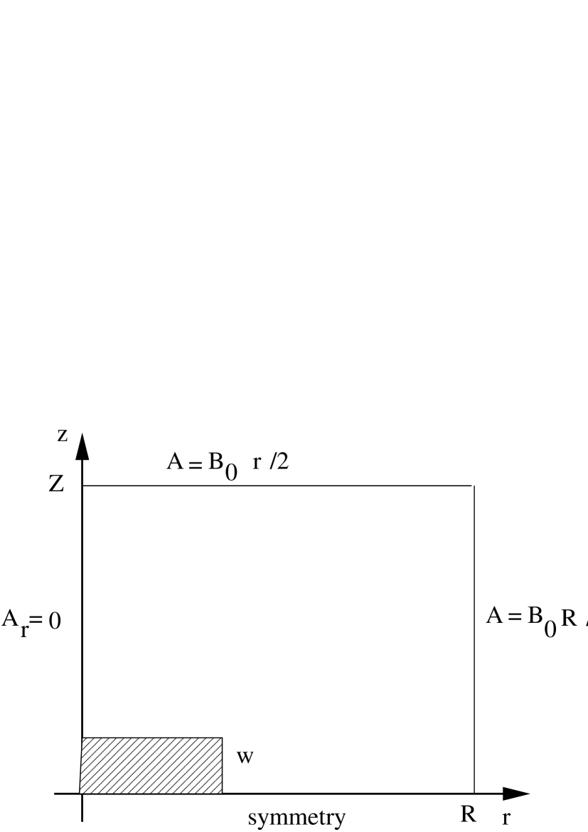
Figure 1: Computational domain for the solution of equation (12) in the $(r,z)$ plane. The boundary conditions are indicated.

We present results obtained by solving equation (12) using the finite element software Comsol [21]. As stressed above, the problem is linear so that $A$ can be scaled arbitrarily. Also the unit of length has been chosen as $mm$ for commodity. Then the dimensions of the sample and the London penetration depth are all given in mm. The London penetration depth we have chosen at 20K is $\lambda=1.610^{-4}mm$. It is in the range of the measurements reported in [22]. Concerning the boundary conditions in Fig. 1 we stress that the position of the boundary $z=Z=40$ is arbitrary. It corresponds to a value for which the screening field has decayed enough so that $B=B_{0}$. Fig. 2 presents a typical result of the magnetic field $B$ for an applied field $B_{0}=1$ for the disk geometry $D_{1}$ (see Table 1 below). Since the problem is linear, the magnitude of $B_{0}$ can be chosen arbitrarily. $B$ ranges from 0 to 2.4 and is near zero in the superconductor. The curvature of the flux-lines outside the superconductor reduces the induction field near the upper surface of the superconductor. This effect is reinforced as the radius of the disks increases. We emphasize the field reinforcement at the boundary $r=9.75$ mm of the disk. In fact the field at the interface is singular in this model because of the jump in $\nabla A$.

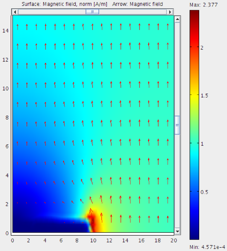
Figure 2: Numerical integration of the Maxwell/London equation (12) showing $B$ as a vector field for the disk geometry $D_{1}$ with $|B_{0}|=1$.

This model allows to calculate the magnetic induction field distribution everywhere around a superconducting sample. It avoids the complications arising from the computation of the demagnetizing field, even when the external field is inhomogeneous. However, the main advantage of this model is the possibility to solve the inverse problem of designing a magnetic shield using as a starting constraint the external applied field and the geometry of the region to be shielded. Of course this approach can be rigorously applied when the flux density penetration in the sample can be disregarded. However, for initial vortex penetration at the surfaces in large geometries as expected for shielding applications, the outside field will not be radically different from the one calculated using our approach. This is due to geometric effects resulting from the Laplacian equation or, in other words, to the demagnetizing energy of the bulk Meissner state. We will come back to this point below.

3 Samples fabrication and characterization technique

Three disk-shaped MgB₂ samples were fabricated by non-conventional Spark Plasma Sintering (SPS) [23]. Their dimensions are reported in Table I.

disk	diameter (mm)	thickness (mm)
$D_{1}$	19.5	1.9
$D_{2}$	14.8	1.75
$D_{3}$	8.1	1.8

Table 1: Dimensions of the three disks analyzed.

The samples were fabricated by pouring the commercially available MgB₂ powder [24] into a graphite mould, that was placed into the working chamber that was evacuated down to a pressure of 1 mbar. A pulsed electric current (2000 A, 4 V) was passed through the sample while the temperature was raised to 1200^∘C in 7 min. The samples were kept at this temperature for 5 min under a 50 MPa uniaxial pressure. Finally, they were cooled down to room temperature in 8 min. The disks obtained were rectified by mirror polishing using pure ethanol as a lubricant. The relative density of the samples was more than 98 % of the theoretical value, their Vickers hardness was 1050 MPa and their critical temperature was T_c = 37 K.

The measures were carried out at a temperature of 20 K in a uniform dc magnetic field up to 1.5 T. These fields are applied in the $z$ direction, perpendicularly to the sample surface. They are generated by a superconducting cryogen free coil coaxial to the samples. The samples were mounted on the top of the second cooling stage of a cryocooler with an interposed 0.125 mm thick indium sheet in order to guarantee a good thermal contact to avoid thermo-magnetic instabilities causing flux jumps [25, 26]. These would strongly modify the shielding capability of the sample and, in the worst case, could create cracks and irreversible damage. A schematic view of the experimental set-up is reported in [27].

The $z$ component of the magnetic induction, i.e. the component parallel to the applied magnetic field direction, was measured with a GaAs Hall probe array mounted on the bottom surface of a custom-designed motor-driven stage, able to be moved along the sample axis with a spatial resolution of 1$\mu$m. Each probe has a disk-shaped active area with a diameter of 300 $\mu$m and an average sensitivity of 43.2 mV/T for a bias current of 0.1 mA. The probes were aligned along the sample diameter following the radial arrangement reported in Fig. 3.

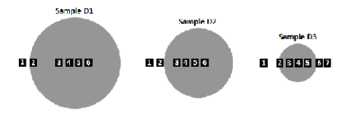
Figure 3: Hall probe arrays for measuring the $z$ component of the magnetic field for the three samples of table I.

The radial positions are detailed in table II for each sample.

disk	radius	d	d	d	d	d	d	d
D1	9.75	-11.2	-9.8	-3.2	-1.2	0.8	2.8
D2	7.4	-10.5	-8.2	-4.7	-2.7	-0.7	1.3
D3	4.05	-7.4	-3.9	-1.9	0.1	2.1	4.6	6.4

Table 2: Radial distance of the probes from the center for each sample. All the dimensions are in mm; the error in the position of each probe is about 0.2 mm.

The sample temperature, the applied magnetic field, the Hall probe positioning and the Hall voltage were controlled with a Labview^TM custom program. The experiments were performed after a zero-field cooling. The magnetic field was gradually increased up to a predetermined value. The induction field profiles were recorded for different distances $z$ above the sample.

4 Analysis of the experimental data

An important consequence of the London approximation is that the model is linear so the results should scale with the magnetic field $B_{0}$. We have tested this scaling on the experimental data for the three disks analyzed. The main result is that for all three samples the experimental curves scale as $B/B_{0}$ as long as $B_{0}<$ 0.4T. The scaling is perfect up to 0.1T and above that value there are small differences especially close to the center of the disk. It is worthwhile to remember that the data refer only to the $z$ component of the field $B$.

We first show the results for a small applied field $B_{0}<$ 0.1T. In Fig. 4 we present $B/B_{0}$ as a function of the distance $z$ from the superconductor surface for $B_{0}$ = 0.04T, 0.07T and 0.1T at different radial positions for the three samples $D_{1},~{}D_{2},~{}D_{3}$. In the following whenever we consider measurements $z$ will refer to the distance above the superconductor.

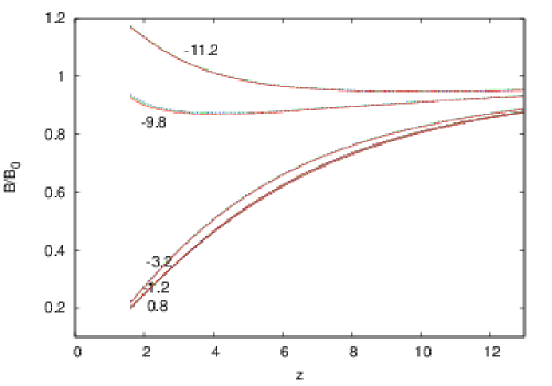
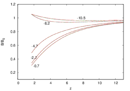
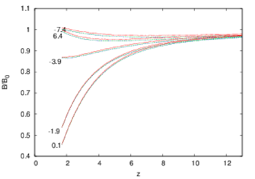
Figure 4: Plot of $B/B_{0}$ as a function of the distance above the superconductor $z$ for $B_{0}$ = 0.04T (continuous line, red online), for $B_{0}$ = 0.07T (long dashed line, green online) and $B_{0}$ = 0.1T (short dashed line, blue online) and for different radial positions. The three panels correspond to the three samples $D_{1},~{}D_{2},~{}D_{3}$ from top to bottom.

As expected there is a very good scaling. The shielding effect is maximum in correspondence to the sample center, increases with sample diameter and decreases towards the edges. The upper curvature of the field lines detected near the samples by the outer Hall probes is due to the demagnetization effects at the disk edges [9]. It is more pronounced in the sample D₁ because it has the largest diameter.

When the applied field is increased up to 0.4T the scaling remains quite good even if some discrepancies start emerging. We show in Fig. 5 the ratio $B/B_{0}$ as a function of $z$ for $B_{0}$ = 0.1T, 0.2T and 0.4T. Again the three panels correspond to the three samples.

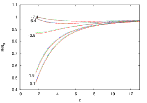
Figure 5: Plot of $B/B_{0}$ as a function of $z$ for $B_{0}$ = 0.1T (continuous line, red online), 0.2T (long dashed line, green online) and 0.4T (short dashed line, blue online) and for different radial positions. The three panels correspond to the three samples $D_{1},~{}D_{2},~{}D_{3}$ from top to bottom.

These results confirm that a linear theory such as the Maxwell/London equation can describe well the disk data for magnetic fields smaller than 0.4T at 20K.

We now use these values of $B_{0}$ to compare the solution of the London equation (5) with the experimental data. The results are shown in Fig. 6 for the disk sample $D_{1}$. There the experimental data are shown as lines for clarity. Only the value $B_{0}$ = 0.1T is presented since we have a good scaling $B/B_{0}$ as shown previously. The agreement is good for small and large $r$ values.

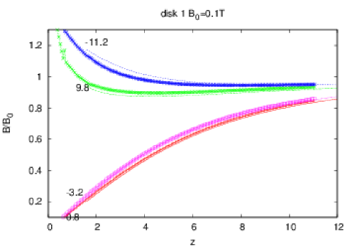
Figure 6: Comparison between the ratio $B/B_{0}$ calculated and measured for sample D₁ as a function of the distance $z$ above the superconductor for different $r$. The measurement temperature was T=20K and $B_{0}$ = 0.1T. The experimental data are shown with lines and the numerical values are plotted with symbols. The different values of $r$ are reported in the figure.

For the disks 2 and 3, we observe a similar trend as shown in Figs. 7 and 8.

Figure 7: Comparison between the ratio $B/B_{0}$ calculated and measured for sample D₂ as a function of $z$ and for different $r$. The other parameters are the same as in Fig. 6.

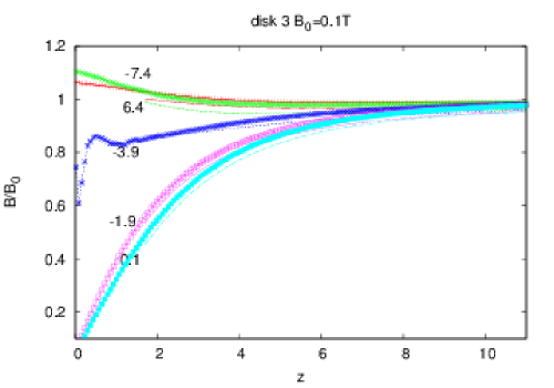
Figure 8: Comparison between the ratio $B/B_{0}$ calculated and measured for sample D₃ as a function of $z$ and for different $r$. The other parameters are the same as in Fig. 6.

When the field $B_{0}$ is increased, vortices penetrate the sample so that the phase cannot be considered as uniform. Then the vector potential $A$ does not depend linearly on the applied field $B_{0}$. This effect is stronger for the small sample $D_{3}$ because it does not screen the field as well as $D_{1}$ does. Fig. 9 shows the region close to the samples for $D_{1}$ (top panel), $D_{2}$ (middle panel) and $D_{3}$ (bottom panel).

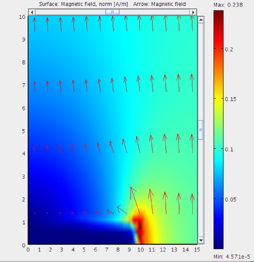
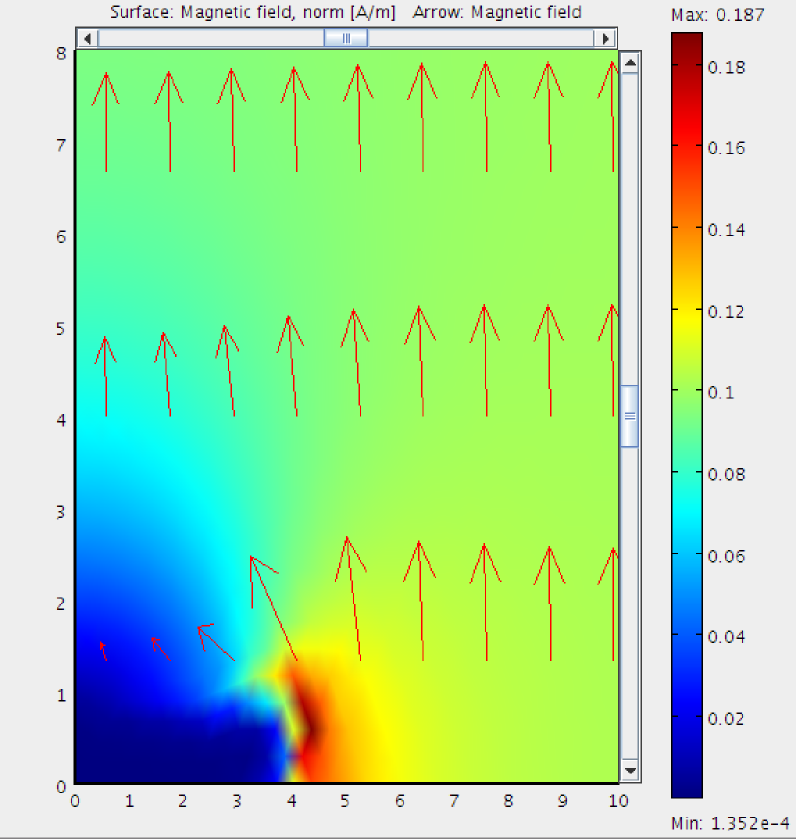
Figure 9: Blow-up of the region close to the samples showing how screening is enabled. The magnetic induction field $\mathbf{B}$ is shown with arrows and its magnitude is in the colour code. The three samples are $D_{1}$ (top), $D_{2}$ (middle) and $D_{3}$ (bottom). The maximum of $|\mathbf{B}|$ in dark red (online) is 0.24 for $D_{1}$, 0.22 for $D_{2}$ and 0.19 for $D_{3}$. The $z$ range is $z<10$ (top panel) and $z<8$ (middle and bottom panels). The applied field is $B_{0}=0.1$.

The screening region where the field is close to zero is a triangle $z<R_{1}/2-0.3r$ for the sample $D_{1}$, $z<R_{2}/2-0.43r$ for the sample $D_{2}$ and $z<R_{3}/2-0.5r$ for the sample $D_{3}$. This screened region by disk $D_{1}$ is twice as large as the one screened by disk $D_{3}$. This is a geometric effect that depends on the sample dimensions only.

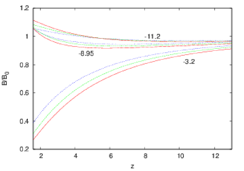
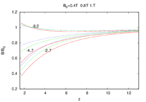
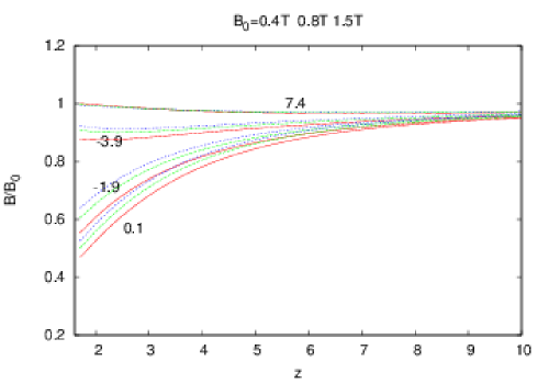
Figure 10: Ratios $B/B_{0}$ as a function of $z$ for $B_{0}$=0.4T (continuous line, red on line), 0.8T (long dashed line, green on line) and 1T (short dashed line, blue on line) and different radial positions. The three panels correspond to samples $D_{1},~{}D_{2},~{}D_{3}$ from top to bottom.

The $B/B_{0}$ ratios shown in Fig. 10 show that the scaling is not so good for $B_{0}$ equal or higher than 0.4T, indicating that for such a large field the vortex penetration inside the sample cannot no longer be disregarded. Nonlinearities appear that can be taken into account in the model.

5 Discussion and Conclusion

From the results shown in the previous section, we see that the Maxwell/London model (5) is appropriate to describe in a simple way the magnetic induction field distribution outside disk-shaped MgB₂ samples at 20K for applied fields lower than 0.4T. From the model, it is easy to compute the shielding field, $\mathbf{B}-\mathbf{B_{0}}$, generated by the disks. We show this field direction in Fig. 11 with the arrows, while the modulus of the total field $\mathbf{B}$ is shown with the color code. The superconductor induces a redistribution of the induction field around itself. In particular, notice the shielding effect above the upper surface of the sample where the superconductor generates a field that is exactly opposed to the applied field. There is also a strong field reinforcement right outside the disk, for $z=0,r>R_{1}$ , where the shielding field is aligned with the applied field.

Figure 11: Screening field $\mathbf{B}-\mathbf{B_{0}}$ of disk $D_{1}$ shown as arrows. The total field, $\mathbf{B}$, is shown with the color code as in Fig. 9.

This magnetic flux distribution allows to design a magnetic screen. This design is a problem of shape optimisation which is difficult to solve in general. A simplification is to assume a shape dependent on a parameter and minimize a criterion with respect to this parameter. The study done on the disk guides us towards an ideal geometry. In particular we want to avoid the regions where the field is reinforced and we want the screening field to remain aligned and opposite the applied field in the screening region. From our calculations and the results reported in the literature[11] we can rule out a cylinder which would exhibit field reinforcement inside the screening region. Instead, a good candidate would be a screen shaped as a cup, see Fig. 12. Inside the cup, the field lines will cause the screening field to be opposite to the applied field.

Figure 12: Schematic drawing of a magnetic screen in the form of a cup of depth $h$.

Then one would minimize the magnetic field $\mathbf{B}$ in a given domain $\Omega$. One could also minimize the magnetic energy in $\Omega$

$${\cal E}={1\over B_{0}^{2}}\int_{\Omega}\mathbf{B}^{2}drdz={1\over B_{0}^{2}}\int_{\Omega}drdz\left[A_{z}^{2}+({1\over r}(rA)_{r})^{2}\right].$$ (17)

To illustrate the procedure we compute the solution for the cup and change the parameter $h$. The domain $\Omega$ is obviously a subset of the cup interior. The numerical procedure is slightly different than for the disk since the geometry does not have mirror symmetry. Instead we apply the same boundary condition (14) at the two extremities $z=\pm Z$. We have chosen $a=3~{}mm,r_{i}=12~{}mm~{},r_{e}=r_{i}+a$ and three different values of the cup depth $h=2~{}mm,4~{}mm$ and 8  $mm$. The sizes were chosen just to demonstrate the object feasibility: of course in a shield fabrication they can be rescaled in order to meet the experimental constraints. We take $B_{0}=1$ so as not to scale the field in equation (17). Since the problem is linear, also in this case the unit is arbitrary. Fig. 13 shows the magnetic field for a cup where $h=4$ mm. The vector field $\mathbf{B}$ is drawn and its modulus is given by the color code. Notice the strong reinforcement at each edge of the cup. The dark region (dark blue online) confirms that the field is very small in the interior of the cup.

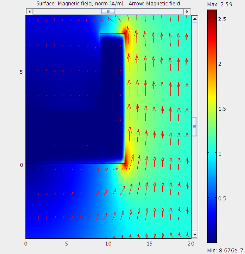
Figure 13: Magnetic induction field direction (arrows) and modulus (in color code) for a cup shield.

As $h$ is increased, the field is reduced inside the cavity. Fig. 14 shows the field in the cavity ($r\leq 9$ mm) for a given $z$ as a function of $r$. The left panel corresponds to $h=4~{}mm$ and $z=3~{}mm,~{}4~{}mm,~{}5~{}mm$ and 6 $mm$ while the right panel is for $h=8~{}mm$ and $z=3~{}mm,~{}5~{}mm,~{}7~{}mm$ and 9 $mm$. We see that for $z<a+2~{}mm$ ($2~{}mm$ above the bottom of the cup) and for $h=4~{}mm$ we have

$$5\%\leq{B\over B_{0}}\leq 10\%.$$

As expected, increasing the height of the cup reduces the field inside the cup. When $h=8~{}mm$ , and $z<a+4~{}mm$ we have

$$1\%\leq{B\over B_{0}}\leq 5\%.$$

Therefore increasing the cup depth, one can completely suppress the magnetic field to a given tolerance. We can then realize a suitable magnetic field screen.

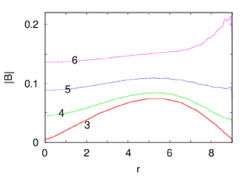
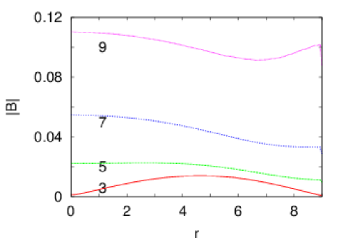
Figure 14: Magnetic induction field modulus inside the cup as a function of $r$ for different values of $z$. Two different cup depths are shown, $h=4$ mm (left panel) and $h=8$ mm (right panel). The values of $z$ are indicated on the figures.

In summary, we have shown that the Maxwell/London model is suitable to describe the magnetic field redistribution induced by a superconducting sample. This approach was validated by comparing the numerical solutions to the values of the induction field measured above disk-shaped MgB₂ samples. At T = 20 K, the agreement is very good for external applied field lower than 0.4 T. This quantitative agreement between experimental results and a simple model is rare in the literature.

The study indicates that the model can be used also above the lower critical field, provided that the penetration of the flux lines inside the sample gives a negligible contribution to the field values outside the superconductor itself.

The model has no adjustable parameters, since the London penetration length is a characteristic of the superconducting material used in the experiment and is introduced a priori. This approach can be used for superconductors of whatever shape; it also applies when the external field is inhomogeneous.

Starting from these results, we demonstrated on a cup geometry, how to design an efficient magnetic field screen by minimizing the magnetic energy in a given region. The simplicity of the direct problem allows to solve this minimization problem easily and therefore find a cup height $h$ so that the average field inside a sub-region of the cup interior is below the tolerance. This is the basis for the design of efficient magnetic field screens.

6 Acknowledgements

J.G. C. thanks Michael Sigal for very helpful discussions. The authors are grateful to the Centre de Ressources Informatiques de Haute Normandie where most of the calculations were done. J. G. C. thanks the Department of Mathematics of the University of Arizona for its hospitality during a sabatical visit.

References

- [1] H. Xia, A. Ben-Amar Baranga, D. Hoffman, and M. V. Romalis, Appl. Phys. Lett. 89, 211104 (2006).
- [2] R. Körber, A. Casey, A. Shibahara, M. Piscitelli, B. P. Cowan, C. P. Lusher, J. Saunders, D. Drung, and Th. Schurig, Appl. Phys. Lett. 91, 142501 (2007).
- [3] G. Delso, S. Ziegler, Eur. J. Nucl. Med. Mol. Imaging 36, S86 (2009).
- [4] O. Baltag, D. Costandache, M. Rau A. Iftemie, I Rau, Adv. Electr. Comput. Eng. 10, 135 (2010).
- [5] R. Harrison, R. Bateman, J. Brown, F. Domptail, C. M. Friend, P. Ghoshal, C. King, A. Van der Linden, Z. Melhem, P. Noonan, A. Twin, M. Field, S. Hong, J. Parrell, and Y. Zhang, IEEE Trans. Appl. Supercond. 18, 540 (2008).
- [6] Y. Seki, D. Suzuki, K. Ogata and K. Tsukada K Appl. Phys. Lett. 82, 940 (2003).
- [7] S Denis , L Dusoulier , M Dirickx , Ph Vanderbemden, R Cloots , M Ausloos and B Vanderheyden, Supercond. Sci.Technol. 20, 192 (2007).
- [8] C.P. Bean, Rev. Mod. Phys. 36, 31 (1964).
- [9] E. H. Brandt, Phys. Rev. B 58, 6506 (1998).
- [10] A. Sanchez and C. Navau, Phys. Rev. B 64, 214506 (2001)
- [11] S Denis , M Dirickx , Ph Vanderbemden , M Ausloos and B Vanderheyden, Supercond. Sci. Technol. 20, 418 (2007).
- [12] J-F Fagnard, M Dirickx, M Ausloos, G Lousberg, B Vanderheyden and Ph Vanderbemden, Supercond. Sci. Technol. 22, 105002 (2009).
- [13] C. Navau, N. Del-Valle and A. Sanchez, IEEE Trans. Appl. Supercond. 23, 8201023 (2013).
- [14] M. Tinkham, ”Introduction to Superconductivity”, second edition, Dover, (2004).
- [15] T. Van Duzer and C. W. Turner, ”Principles of superconductive devices and circuits”, Edward Arnold, (1998).
- [16] M. Tomsic, M. Rindfleisch, J. Yue, K. McFadden, J. Phillips, M. D. Sumption, M. Bhatia, S. Bohnenstiehl, and E. W. Collings, Int. J. Appl. Ceram. Technol., 4, 250 (2007).
- [17] L. Gozzelino, F. Laviano, D. Botta, A. Chiodoni, R. Gerbaldo, G. Ghigo, E. Mezzetti, G. Giunchi, S. Ceresara, and G. Ripamonti, Philos. Mag. B, 82, 1 (2002).
- [18] P. Mikheenko, V. V. Yurchenk and T. H. Johansen, Supercond. Sci. Technol. 25 045009 (2012).
- [19] J.Noudem, P.Bernstein and Y.Thimont, french patent FR 1255988.
- [20] L. Gozzelino, B. Minetti, R. Gerbaldo , G. Ghigo, F. Laviano, G. Lopardo, C. Plapcianu , A. Agostino, J. Supercond. Nov. Magn. 24, 307 (2011).
-
[21]
Comsol Multiphysics modeling and simulation software,
http://www.comsol.com/ - [22] F. Manzano, A. Carrington, N.E. Hussey, S. Lee, A. Yamamoto, and S. Tajima, Phys. Rev. Lett. 88, 047002 (2002).
- [23] FCT System GmbH, HP D25, Rauenstein, Germany.
- [24] H. C. Starck GmbH, Goslar, Germany.
- [25] E. Altshuler and T.H. Johansen, Rev. Mod. Phys. 76, 471 (2004).
- [26] G. Ghigo, R. Gerbaldo, L. Gozzelino, F. Laviano, G. Lopardo, E. Monticone, C Portesi, E. Mezzetti, Appl. Phys. Lett. 94, 052505 (2009).
- [27] L. Gozzelino, B. Minetti, R. Gerbaldo, G. Ghigo, F. Laviano, A. Agostino and E. Mezzetti, IEEE Trans. Appl. Supercond. 21, 3146 (2011).