Ticks, Deer, Mice, and a Touch of Sensitivity: A Recipe for Controlling Lyme Disease

Abstract

Borrelia burgdorferi sensu stricto is a bacterial spirochete prevalent in the Northeastern United States that causes Lyme disease. Lyme disease is the most common arthropod–borne disease in the United States; affecting mice, deer, humans and other mammals. The disease is spread by Ixodes Scapularis, a species of tick whose primary food source are deer and mice. Reducing the population of ticks feeding on both large and small mammals below some critical threshold can decrease the prevalence of Lyme disease among humans. A simplified, six–dimensional Susceptible–Infected, SI, model is used to capture the mice–deer–tick dynamics while considering the impact of varying population–specific death rates on infected population size. We analyzed the stability of the models two equilibria, the unstable disease free equilibrium and the endemic equilibrium. Static forward sensitivity analysis is conducted on the basic reproduction number and the endemic equilibrium. A dynamic approach was explored to observe change in the sensitivity of the death rates over time. These analyses were conducted to determine the efficacy of changing death rates in order to reduce prevalence of Lyme disease.

¹ Applied Mathematics, Northeastern Illinois University, Chicago, Illinois
² Pure Math, University of Florida, Gainsville, Florida
³ Applied Mathematics, Arizona State University, Tempe, Arizona
⁴ Pure Math, University of Wisconsin–Whitewater, Whitewater, Wisconsin

1 Introduction

Lyme disease is an epidemic in the U.S. and is caused by the bacterium, Borrelia burgdorferi Sensu Stricto. B. burgdorferi is transmitted in the Northeast and Midwest by a tick, Ixodes scapularis, and was first discovered in the area of Lyme, Connecticut in 1977 [Specter,]. The disease is heavily concentrated in the Northeast and upper Midwest of the United States; causing victims to exhibit symptoms including fever, headache, fatigue, and a characteristic skin rash called erythema migrans. If left untreated, the infection can spread to joints, the heart, and the nervous system [CDC,]. If properly detected, Lyme disease is usually treated with antibiotics in its early stages and no further complications ensue[A. C. Steere and Malawista, 1983]; however, up to twenty percent of the people infected with Lyme disease exhibit symptoms that can last many years after the treatment. The chronic symptoms, referred to as Post–Treatment Lyme Disease Syndrome (PTLDS) [G. Biesiada et al., 2012], vary but can include muscle and joint pains, cognitive defects, sleep disturbance, fatigue, seizures, and even death. The consequences of Lyme disease and PTLDS are extremely debilitating and can last for years; forcing those affected to depend on others for their most basic daily needs.

Lyme disease is the most commonly reported tick-borne illness in the United States. In 2009, the C.D.C. reported 38,000 documented cases nationwide; three times more than in 1991 [Specter,]. In states such as Delaware, Illinois, Wisconsin, and other neighboring states, the number of cases has tripled from 2002 to 2011. Most researchers agree that the true number of infections is five to ten times higher due to undiagnosed cases. Lyme disease is classified as a zoonosis because transmission to humans from an animal reservoir is carried out by ticks that feed on both parties [S. M. Dunham-Ems and Radolf, 2009].

Adult ticks lay their eggs in the spring after feeding on deer. During the late spring and summer, the larvae feed on small mammals such as and mice who act as natural reservoirs of the B. burgdorferi spirochete [E. M. Bosler and Benach, 1984]. Nymphal ticks also feed on the mouse population with the infected nymphs passing on their infection to their new potentially susceptible host [R. V. Lo 3rd and MacGregor, 2004]. In the final stage of its lifecycle, the adult tick will feed on a large mammal, reproduce, and then die. The deer is the preferred host of the adult I. Scapularis, as these large mammals can easily survive through the winter season.

Lyme disease can spread through fluid transfer, such as a blood transfusion, but is not sexually transmissible and is not passed on to offspring. [Woodrum and Jr, 1999] No consensus exists supporting or refuting the idea that deer can transmit Lyme disease to ticks; even though the spirochete can be found on the skin and in the muscles of deer [P. Bruno and Claudine, 2000]. Furthermore, the majority of studies conducted in this area claim that it is not possible. In this model, we assume deer to tick transmission is negligible, i. e. $\beta_{DT}=0$, where $\beta_{DT}$ represents the contact rate and rate of transmission from deer to tick. The only proven method for control of the disease has been complete eradication of the deer population [Barbour and Fish, 1993]. This course of action was only possible due to the geographical isolation of the community. However, a reduced deer population can lead to exacerbated diseased tick density because they start to feed predominantly on mice. We do not recognize the eradication of deer to be a feasible solution to the problem of Lyme disease. Other strategies have involved attempting to control the interactions between mice and ticks in order to control the infection at its source, an approach attempted using cotton balls laced with a pesticide called permethrin in the dens of the mice. The balls made the mice unattractive as carriers for nymphal ticks [Barbour and Fish, 1993]. This was not a workable solution because the mouse population was so dense that the effect of the cotton balls on the total population was insignificant. Another approach is the vaccination of reservoir hosts against B. Burgdorferi [Barbour and Fish, 1993]. This approach would be effective for a particular reservoir species, but would not be effective given the diversity of the B. burgdorferi reservoir.

Our work reveals a partial solution to the problem by controlling the Lyme disease vector at the host level. Our model looks to show the efficacy of modifying the death rate of one species at reducing populations of the other species. These perturbations in the death rates can be accomplished through harvesting or other prevention methods. Dual reservoirs and a single vector population are incorporated into an SI model in six dimensions.

2 Model & Methods

We construct a single–patch Susceptible–Infected (SI) model ignoring immigration, emigration and seasonality. A removed or recovered class is not incorporated into the model as is typical in SIR models, since infected animals do not recover. Furthermore, all animal and arthropod carriers of Borellia Burgdorferi Sensu Stricto, are asymptomatic; implying no disease-related deaths. We construct a three–tier, bi–compartmental model incorporating the vector and host species. The model yields a six-dimensional system of differential equations describing the evolution of Lyme disease in a population of deer, mice and ticks. We choose a timescale of twenty–four hours per time step, due to the time it takes the bacteria to be transmitted from a tick to a human which is thirty–six to forty–eight hours. [CDC,]

We make several assumptions for the model: we see no vertical transmission of the spirochete in ticks or any of the host species [L. Rollend and Childs, 2013]; it is not spread like a venereal disease, nor is it contagious; and there is no horizontal transmission of B. Burgdorferi at the level of the vectors or the host species [Woodrum and Jr, 1999]. Further, since studies claim that deer are a dilutant host; i.e. they are incapable of transmitting the B. Burgdorferi spirochete to a feeding vector, we assume no transfer of infection from deer to tick [Barbour and Fish, 1993]. This assertion has been lightly contested, so assuming a transfer rate would be an interesting avenue for further study, but is beyond the scope of the current project. Since we find B. Burdorferi present on the skin of deer, we consider an infected deer class , additionally, ticks reproduce on the deer; therefore, we assume that the density of the deer population is positively correlated with the tick reproduction rate. Finally, we assume that the frequency of tick bites per unit time saturates at one. This means that out of all the contacts a given tick will have with potential hosts in a day, it will feed on only one. This allows us to simplify the contact expressions in each of our six equations, thereby simplifying the model.

The six populations described in the model are defined in Table 1:

Table 1: Populations Involved in the Model

State Variable	Meaning
$S_{D}$	Susceptible deer population.
$I_{D}$	Infected deer population.
$S_{M}$	Susceptible mouse population.
$I_{M}$	Infected mouse population.
$S_{T}$	Susceptible tick population.
$I_{T}$	Infected tick population.

In the following table, (Table LABEL:table:variables), population densities are per square kilometer. The parameter values that we use have been acquired from census data, the CDC, hunting reports, and also from various studies conducted in the field.

Table 2: Definition of the variables in the modeling framework

Parameter	Meaning	Units	Value
$D$	Total population of deer	Individuals	300
$M$	Total population of mice	Individuals	3500
$T$	Total population of ticks	Individuals	1530000
$S_{D}$	Susceptible deer	Individuals	216
$I_{D}$	Infected deer	Individuals	84
$S_{M}$	Susceptible mice	Individuals	1050
$I_{M}$	Infected mice	Individuals	2450
$S_{T}$	Susceptible tick	Individuals	979200
$I_{T}$	Infected Ticks	Individuals	550800
$\Lambda_{D}$	Birth/recruitment rate of deer	Individuals/time	$0.147945205\pm?$
$\Lambda_{M}$	Birth/recruitment rate of mice	Individuals/time	$5.4*10^{-}2\pm?$
$\Lambda_{T}$	Birth/recruitment rate of tick	Individuals/time	$2.6*10^{-}2\pm?$
$\beta_{TD}$	Transmission rate from ticks to susceptible deer	1/time	$1.3699*10^{-}3\pm?$
$\beta_{TM}$	Transmission rate from ticks to susceptible mice	1/time	$2.739*10^{-}3\pm?$
$\beta_{MT}$	Transmission rate from mice to susceptible ticks	1/time	$1.863*10^{-}3\pm?$
$\mu_{D}$	Natural death rate for deer	1/time	$4.9*10^{-}4\pm?$
$\mu_{M}$	Natural death rate for mice	1/time	$2.7*10^{-}3\pm?$
$\mu_{T}$	Natural death rate for ticks	1/time	$9.6*10^{-}3\pm?$

The assumptions and definitions lead to the following model on the dynamics of deer–mice–ticks:

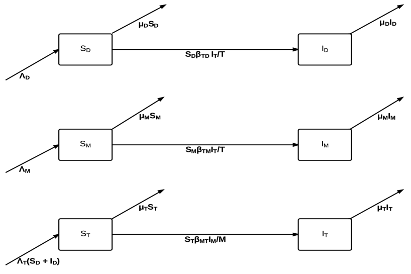
Figure 1: Compartmental Model

$${}\quad\begin{cases}\dot{S}_{D}=\Lambda_{D}-\beta_{TD}\dfrac{I_{T}}{T}S_{D}-\mu_{D}S_{D}\vspace{1.5mm},\\ \dot{I}_{D}=\beta_{TD}\dfrac{I_{T}}{T}S_{D}-\mu_{D}I_{D}\vspace{1.5mm},\\ \dot{S}_{M}=\Lambda_{M}-\beta_{TM}\dfrac{I_{T}}{T}S_{M}-\mu_{M}S_{M}\vspace{1.5mm}\\ \dot{I}_{M}=\beta_{TM}\dfrac{I_{T}}{T}S_{M}-\mu_{M}I_{M}\vspace{1.5mm}\\ \dot{S}_{T}=\Lambda_{T}D-\beta_{MT}S_{T}\dfrac{I_{M}}{M}-\mu_{T}S_{T}\vspace{1.5mm}\\ \dot{I}_{T}=\beta_{MT}S_{T}\dfrac{I_{M}}{M}-\mu_{T}I_{T}\vspace{1.5mm}\\ \end{cases}$$ (1)

Where: $D=S_{D}+I_{D}$, $T=S_{T}+I_{T}$ and $M=S_{M}+I_{M}$

In the equations in (1), where $i\neq j=D,M,T$, the susceptible population that gets infected moves into the infected class with a per capita rate of $\beta_{ij}\dfrac{I_{i}}{i}$. $\beta_{ij}$ is the contact rate and rate of transmission of the spirochete from population $i$ to population $j$. The $\dfrac{I_{i}}{i}$ represents the proportion of infected members of population $i$ that a given individual in population $j$ encounters. The susceptible and infected individuals also leave their respective classes through death according to the terms $\mu_{i}S_{i}$ and $\mu_{i}I_{i}$ respectively. The terms $\mu_{i}$ represent the per capita death rate of population $i$ in each time step. New individuals are recruited into the susceptible population via $\Lambda_{i}$, which represents the number of units of population $i$ that are born in each time step. Note that $\Lambda_{D}$ and $\Lambda_{M}$ are constant while $\Lambda_{T}$ is dependent on the density of deer.

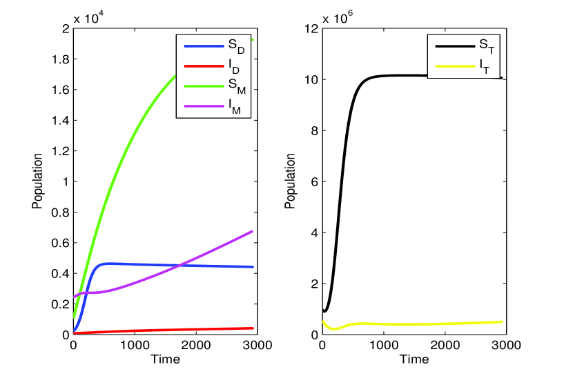
Figure 2: Population Dynamics

The simulation (2) was run over a period of 3000 days to observe the long–term and transient behavior of the model incorporating the initial conditions listed in Table LABEL:table:variables.

3 Disease-Free and Endemic Equilibria and Their Stability

3.1 Disease-Free Equilibria and Stability

The Disease–Free equilibrium (DFE) occurs when the pathogen has suffered extinction and every individual of the population is susceptible. Therefore, in the system (1) we compute the disease–free equilibrium by setting $\text{I}_{D}=0$, $\text{I}_{M}=0$ and $\text{I}_{T}=0$.

The system (1) has a disease free equilibrium denoted by $E_{0}$, where

$$E_{0}=[S_{D}\to\frac{\Lambda_{D}}{\mu_{D}},\text{I}_{D}\to 0,S_{M}\to\frac{\Lambda_{M}}{\mu_{M}},\text{I}_{M}\to 0,S_{T}\to\frac{\Lambda_{D}\Lambda_{T}}{\mu_{D}\mu_{T}},\text{I}_{T}\to 0]$$

The basic Reproduction number, $\mathcal{R}_{0}$, represents the number of new infections one case generates on average over the course of its infectious period.

In order to compute $\mathcal{R}_{0}$, we use the next generation matrix [O. Diekmann and Metz, 1990] and obtain the following:

$$X=\begin{pmatrix}\text{I}_{D}\\ \text{I}_{M}\\ \text{I}_{T}\\ \end{pmatrix}\qquad\text{, }\qquad Y=\begin{pmatrix}\text{S}_{D}\\ \text{S}_{M}\\ \text{S}_{T}\\ \end{pmatrix}$$

Where $X$ is the vector of infected classes and Y the vector of uninfected classes

The original system of equations can be rewritten in the following generalized form:

$\dfrac{\partial X}{\partial t}=\mathcal{F}(X,Y)-\mathcal{V}(X,Y)$

$$\mathcal{F}=\begin{pmatrix}\frac{\text{S}_{D}\text{I}_{T}\beta_{\text{TM}}}{\text{I}_{T}+\text{S}_{T}}\\ \frac{\text{I}_{T}S_{M}\beta_{\text{TM}}}{\text{I}_{T}+S_{T}}\\ \frac{\text{I}_{M}\beta_{\text{MT}}S_{T}}{\text{I}_{M}+S_{M}}\\ \end{pmatrix}\qquad\text{ , }\qquad\mathcal{V}=\begin{pmatrix}\mu_{D}S_{D}\\ \mu_{M}I_{M}\\ \mu_{T}I_{T}\\ \end{pmatrix}$$

Let $F=J(\mathcal{F})$ and $V=J(\mathcal{V})$, where $J$ denotes the Jacobian. Next, compute the eigenvalues of the associated matrix $FV^{-1}$. The reproduction number will be the largest eigenvalue of the Jacobian, thus:

$$\mathcal{R}_{0}=\sqrt{\dfrac{\beta_{TM}\beta_{MT}}{\mu_{M}\mu_{T}}}$$ (2)

Theorem 1.

If $\mathcal{R}_{0}<1$, then the disease free equilibrium, $E_{0}$, is locally asymptotically stable for the system (1). If $\mathcal{R}_{0}>1$, then $E_{0}$ is unstable. [den Driessche and Watmough, 2002]

If $\mu_{M}\mu_{T}\leq\beta_{TM}\beta_{MT}$, then $\mathcal{R}_{0}>1$, thus the DFE will be unstable.

3.2 Endemic Equilibria and Stability

The Endemic Equilibrium of the model is obtained by considering the infectious classes to be greater than zero. The following Endemic Equilibrium is obtained:

$$E^{*}=(S^{*}_{D},I^{*}_{D},S^{*}_{M},I^{*}_{M},S^{*}_{T},I^{*}_{T}),$$

Where,

$$S^{*}_{D}=\frac{\Lambda_{D}\beta_{\text{TM}}\left(\beta_{\text{MT}}+\mu_{T}\right)}{\mu_{T}\left(\mu_{D}\beta_{\text{TM}}-\mu_{M}\beta_{\text{TD}}\right)+\beta_{\text{MT}}\beta_{\text{TM}}\left(\mu_{D}+\beta_{\text{TD}}\right)},$$

$$I^{*}_{D}=\frac{\Lambda_{D}\beta_{\text{TD}}\left(\beta_{\text{MT}}\beta_{\text{TM}}-\mu_{M}\mu_{T}\right)}{\mu_{D}\left(\mu_{T}\left(\mu_{D}\beta_{\text{TM}}-\mu_{M}\beta_{\text{TD}}\right)+\beta_{\text{MT}}\beta_{\text{TM}}\left(\mu_{D}+\beta_{\text{TD}}\right)\right)},$$

$$S^{*}_{M}=\frac{\Lambda_{M}\left(\beta_{\text{MT}}+\mu_{T}\right)}{\beta_{\text{MT}}\left(\mu_{M}+\beta_{\text{TM}}\right)},\text{I*}_{M}=\frac{\Lambda_{M}\left(\beta_{\text{MT}}\beta_{\text{TM}}-\mu_{M}\mu_{T}\right)}{\mu_{M}\beta_{\text{MT}}\left(\mu_{M}+\beta_{\text{TM}}\right)},$$

$${S^{*}}_{T}=\frac{\Lambda_{D}\Lambda_{T}\left(\mu_{M}+\beta_{\text{TM}}\right)}{\mu_{D}\beta_{\text{TM}}\left(\beta_{\text{MT}}+\mu_{T}\right)},\text{I*}_{T}=\frac{\Lambda_{D}\Lambda_{T}\left(\beta_{\text{MT}}\beta_{\text{TM}}-\mu_{M}\mu_{T}\right)}{\mu_{D}\mu_{T}\beta_{\text{TM}}\left(\beta_{\text{MT}}+\mu_{T}\right)}.$$

It is important to note that the reproductive number is present in the numerator of the infected terms of the endemic equilibrium, thus the infected populations are higher if the reproductive number is larger. The reproductive number, as well as the endemic equilibria depend on transmission rates between mice and ticks as well as the death rates of both populations.

Theorem 2.

The system (1) has a unique endemic equilibrium, $E^{*}=(S^{*}_{D},I^{*}_{D},S^{*}_{M},I^{*}_{M},S^{*}_{T},I^{*}_{T})$, iff $\mathcal{R}_{0}>1$ and $\mathcal{R}_{0}>\mathcal{R}_{1}$, where $\mathcal{R}_{1}=\frac{\mu_{M}\beta_{TD}-\mu_{D}\beta_{TM}}{(\mu_{D}+\beta_{TD}\mu_{M})}$. The endemic equilibrium $E^{*}$ is locally asymptotically stable whenever it exists.

In order to verify stability we compute the Jacobian evaluated at the endemic equilibrium:

$$J|_{E^{*}}=\left(\begin{array}[]{cccccc}-\frac{\text{I}_{T}\beta_{\text{TD}}}{\text{I}_{T}+S_{T}}-\mu_{D}&0&0&0&\frac{\text{I}_{T}S_{D}\beta_{\text{TD}}}{\left(\text{I}_{T}+S_{T}\right){}^{2}}&-\frac{S_{D}S_{T}\beta_{\text{TD}}}{\left(\text{I}_{T}+S_{T}\right){}^{2}}\\ \frac{\text{I}_{T}\beta_{\text{TD}}}{\text{I}_{T}+S_{T}}&-\mu_{D}&0&0&-\frac{\text{I}_{T}S_{D}\beta_{\text{TD}}}{\left(\text{I}_{T}+S_{T}\right){}^{2}}&\frac{S_{D}S_{T}\beta_{\text{TD}}}{\left(\text{I}_{T}+S_{T}\right){}^{2}}\\ 0&0&-\frac{\text{I}_{T}\beta_{\text{TM}}}{\text{I}_{T}+S_{T}}-\mu_{M}&0&\frac{\text{I}_{T}S_{M}\beta_{\text{TM}}}{\left(\text{I}_{T}+S_{T}\right){}^{2}}&-\frac{S_{M}S_{T}\beta_{\text{TM}}}{\left(\text{I}_{T}+S_{T}\right){}^{2}}\\ 0&0&\frac{\text{I}_{T}\beta_{\text{TM}}}{\text{I}_{T}+S_{T}}&-\mu_{M}&-\frac{\text{I}_{T}S_{M}\beta_{\text{TM}}}{\left(\text{I}_{T}+S_{T}\right){}^{2}}&\frac{S_{M}S_{T}\beta_{\text{TM}}}{\left(\text{I}_{T}+S_{T}\right){}^{2}}\\ \Lambda_{T}&\Lambda_{T}&\frac{\text{I}_{M}S_{T}\beta_{\text{MT}}}{\left(\text{I}_{M}+S_{M}\right){}^{2}}&-\frac{S_{M}S_{T}\beta_{\text{MT}}}{\left(\text{I}_{M}+S_{M}\right){}^{2}}&-\frac{\text{I}_{M}\beta_{\text{MT}}}{\text{I}_{M}+S_{M}}-\mu_{T}&0\\ 0&0&-\frac{\text{I}_{M}S_{T}\beta_{\text{MT}}}{\left(\text{I}_{M}+S_{M}\right){}^{2}}&\frac{S_{M}S_{T}\beta_{\text{MT}}}{\left(\text{I}_{M}+S_{M}\right){}^{2}}&\frac{\text{I}_{M}\beta_{\text{MT}}}{\text{I}_{M}+S_{M}}&-\mu_{T}\\ \end{array}\right)$$ (3)

Which yields the following eigenvalues:

$$\begin{array}[]{cccc}\lambda_{1}=-\mu_{D}\\ \lambda_{2}=-\mu_{T}\\ \lambda_{3}=-\mu_{M}\\ \lambda_{4}=\frac{\mu_{T}\left(\mu_{M}\beta_{\text{TD}}-\mu_{D}\beta_{\text{TM}}\right)-\beta_{\text{MT}}\beta_{\text{TM}}\left(\mu_{D}+\beta_{\text{TD}}\right)}{\beta_{\text{TM}}\left(\beta_{\text{MT}}+\mu_{T}\right)}\\ \end{array}$$ (4)

The first three eigenvalues are negative and $\lambda_{4}<0$ when $\mathcal{R}_{0}>\mathcal{R}_{1}$. $\lambda_{5,6}$ are the solutions the quadratic equation of the form $A\lambda_{5,6}^{2}+B\lambda_{5,6}+C=0$, where:

$A=\left(\mu_{M}+\beta_{\text{TM}}\right)\left(\beta_{\text{MT}}+\mu_{T}\right)$,

$B=\beta_{\text{MT}}\left(\left(\mu_{M}+\beta_{\text{TM}}\right){}^{2}+2\mu_{T}\beta_{\text{TM}}\right)+\beta_{\text{MT}}^{2}\beta_{\text{TM}}+\mu_{T}^{2}\beta_{\text{TM}})$

$C=\left(\mu_{M}+\beta_{\text{TM}}\right)\left(\beta_{\text{MT}}+\mu_{T}\right)\left(\beta_{\text{MT}}\beta_{\text{TM}}-\mu_{M}\mu_{T}\right)$

It is clear that $A$ and $B$ are always greater than zero. When $\mathcal{R}_{0}>1$, the following condition holds $\mu_{M}\mu_{T}\leq\beta_{TM}\beta_{MT}$. It follows that $C$ will always be greater than or equal to zero while $\mathcal{R}_{0}>1$. Therefore, the square root of the discriminant will be between zero and $B$. Thus, the two eigenvalues of the form $\dfrac{-B\pm\sqrt{B^{2}-4AC}}{2A}$ are less than zero when $R_{0}>1$ and the equilibrium is locally stable.

4 Sensitivity Analysis

The basic tenet of sensitivity analysis is that perturbations to the input parameters of a model produce perturbations in the output. Sensitivity analysis quantifies these uncertainties. The quantification is defined as the ratio of a 1 percent change change in the parameter produces what percent change in the output. In our case, the quantities of interest are both static and dynamic. Specifically, the reproduction number and the equilibrium points are static in nature, whereas the dynamic model consisting of the ODEs given in equations (1) is temporal. Sensitivity of the reproduction number describes, via each relevant parameter, how many secondary infections are incurred given a single infection in a completely susceptible population. Sensitivity of the equilibrium points describes how the long–term solutions are affected by changes in the defining parameters. Lastly, sensitivity of the ODE model describes the transient sensitivity. With time dependent models, it is possible for certain parameters to exchange relative importance. For example, parameter $p_{1}$ may be more important then parameter $p_{2}$ up to some crossover time $t_{c}$. After $t_{c}$, parameter $p_{2}$ is more important than $p_{1}$.

Consider a generic model, as shown here, called the forward problem. It takes nominal input parameters, such as $\mu_{\text{D}}$, etc.., which we will refer to as $p$, and generates a solution $u$.

Figure 3: Forward problem consists of generic input(s) $p$ and corresponding output(s) $u$.

Forward sensitivity analysis introduces perturbations to the input parameters, via $\delta p$ and quantifies the subsequent perturbations to the output solution via $\delta u$.

Figure 4: Forward sensitivity quantifies how perturbations $\delta p$ to the input parameter $p$ produces perturbations of the output $\delta u$.

In order to quantify the concept of sensitivity, we define the normalized indices. The normalized sensitivity index is defined to be the limit of the ratio [Arriola and Hyman, 2009]

$$SI(u;p):=\lim_{\delta p\to 0}\displaystyle\frac{\left(\displaystyle\frac{\delta u}{u}\right)}{\left(\displaystyle\frac{\delta p}{p}\right)}=\displaystyle\frac{p}{u}\displaystyle\frac{\partial u}{\partial p}\qquad u\neq 0.$$

These indices essentially gives the percent change in output for a given percent change to the input parameter.

4.1 Sensitivity of the Reproductive Number

The basic reproductive number measures the number of secondary infections created by a single infected tick/mouse in a completely susceptible population. For our model, this metric depends on the following variables: $\mu_{M}$, $\beta_{TM}$, $\beta_{MT}$ and $\mu_{T}$. The parameters that can feasibly be modified are the death rates of the mice, and possibly the tick population; though the latter would be considerably more difficult. The sensitivity analysis on the reproductive number is done to understand the impact on the individual populations of perturbing the death rate of the mice and the death rate of the tick population on the spread of the disease. Calculating the normalized sensitivity index of $\mathcal{R}_{0}$ with respect to $\mu_{M}$ and $\mu_{T}$ indicate that:

$$SI(\mathcal{R}_{0},\mu_{M}) :=SI(\mathcal{R}_{0},\mu_{T})$$

$$=\dfrac{\mu_{M}}{\mathcal{R}_{0}}\dfrac{\partial\mathcal{R}_{0}}{\partial\mu_{M}}$$

$$=\dfrac{\mu_{T}}{\mathcal{R}_{0}}\dfrac{\partial\mathcal{R}_{0}}{\partial\mu_{T}}$$

$$=-\dfrac{1}{2}$$

Thus, if we increase the death rate of the mice (or Ticks) by one percent, the reproductive number will decrease by 0.5%. Similar calculations show:

$$SI(\mathcal{R}_{0},\beta_{TM}) :=SI(\mathcal{R}_{0},\beta_{MT})$$

$$=\dfrac{\beta_{TM}}{\mathcal{R}_{0}}\dfrac{\partial\mathcal{R}_{0}}{\partial\beta_{TM}}$$

$$=\dfrac{\beta_{MT}}{\mathcal{R}_{0}}\dfrac{\partial\mathcal{R}_{0}}{\partial\beta_{MT}}$$

$$=\dfrac{1}{2}$$

Thus decreasing the transmission rates between Ticks and Mice (and vice-versa), by one percent, will decrease the reproductive number by 0.5%.

4.2 Sensitivity of the Endemic Equilibrium

We explored the sensitivities of endemic equilibrium infectious hosts/vector densities to perturbations in death rates of each class. This was done in order to simulate and observe the effects of introducing preventative measures to one of the host populations.

We performed forward sensitivity analysis on the forward problem at the endemic equilibrium in order to acquire normalized sensitivity conditions with respect to each population parameter. We calculated the normalized sensitivity conditions of the species–specific death rates with respect to the populations according to the process previously described:

4.2.1 Normalized Sensitivity Conditions with respect to $\mu_{D}$

$$SI(I_{D};\mu_{D}) =-{\frac{{\beta_{MT}}\,{\beta_{TD}}\,{\beta_{TM}}+2\,{\beta_{TM}}\,{\mu_{D}}\,{\it\beta_{MT}}-{\beta_{TD}}\,{\mu_{M}}\,{\mu_{T}}+2\,{\beta_{TM}}\,{\mu_{D}}\,{\mu_{T}}}{{\beta_{MT}}\,{\beta_{TD}}\,{\beta_{TM}}+{\beta_{TM}}\,{\mu_{D}}\,{\beta_{MT}}-{\beta_{TD}}\,{\mu_{M}}\,{\mu_{T}}+{\beta_{TM}}\,{\mu_{D}}\,{\mu_{T}}}}$$

$$=-\frac{R_{0}(\beta_{TD}+2\mu_{D})\mu_{M}-(\beta_{TD}\mu_{M}+2\beta_{TM}\mu_{D})}{R_{0}(\beta_{TD}+\mu_{D})\mu_{M}-(\beta_{TD}\mu_{M}+\beta_{TM}\mu_{D})}$$

$$=-\frac{\beta_{TD}\mu_{M}(R_{0}-1)+2R_{0}(\mu_{M}-\beta_{TM})\mu_{D}}{\beta_{TD}\mu_{M}(R_{0}-1)+R_{0}(\mu_{M}-\beta_{TM})\mu_{D}}$$

$$SI(I_{M};\mu_{D}) =0$$

$$SI(I_{T};\mu_{D}) =-1$$

From the equations, we can see that increasing Deer death rates always has a negative impact on $I_{T}$ densities. Interestingly, the this parameter does appear not dampen infected mice population (i.e. sensitivity index is zero). We note in passing that this is likely a consequence of our first order approximation of $\frac{\partial I_{M}}{\partial\mu_{D}}$. Finally, we observe that the sensitivity index of the infected Deer class may be positive or negative depending on the relative magnitude of $R_{0}$. Thus we conlcude that $\mu)_{D}$ has its greatest effect on $I_{D}$ but it always has a negative effect on $I_{T}$

4.2.2 Normalized Sensitivity Conditions with respect to $\mu_{M}$

$$SI(I_{D};\mu_{M}) =-{\frac{{\mu_{T}}\,\left({\beta_{MT}}+{\mu_{T}}\right){\beta_{TM}}\,{\mu_{M}}\,{\mu_{D}}}{\left({\beta_{MT}}\,{\beta_{TD}}\,{\beta_{TM}}+{\beta_{MT}}\,{\beta_{TM}}\,{\mu_{D}}-{\beta_{TD}}\,{\mu_{M}}\,{\mu_{T}}+{\beta_{TM}}\,{\mu_{D}}\,{\mu_{T}}\right)\left({\beta_{TM}}\,{\beta_{MT}}-{\mu_{M}}\,{\mu_{T}}\right)}}$$

$$=-\frac{(\beta_{MT}+\mu_{T})\beta_{TM}\mu_{D}\mu_{M}}{\left(R_{0}(\beta_{TD}+\mu_{M})\mu_{M}-(\beta_{TD}\mu_{M}-\beta{TM}\mu_{D})\right)(R_{0}-1)}$$

$$SI(I_{M};\mu_{M}) =-{\frac{{\beta_{MT}}\,{{\beta_{TM}}}^{2}+2\,{\beta_{MT}}\,{\beta_{TM}}\,{\mu_{M}}-{\mu_{T}}\,{{\mu_{M}}}^{2}}{\left({\beta_{TM}}+{\mu_{M}}\right)\left(R_{0}-1\right)\mu_{M}\mu_{T}}}$$

$$=-\frac{R_{0}(\beta_{TM}+2\mu_{M})-\mu_{M}}{(\beta_{TM}+\mu_{M})(R_{0}-1)}$$

$$SI(I_{T};\mu_{M}) =-{\frac{{\mu_{M}}\,{\mu_{T}}}{{\beta_{TM}}\,{\beta_{MT}}-{\mu_{M}}\,{\mu_{T}}}}$$

$$=-\frac{1}{R_{0}-1}$$

From the equations, we observe that the sensitivity of the infected Deer class can also vary depending on the disease dynamics near equilibrium. If $R_{0}>>1$ (and the endemic equilibrium exits), then increasing mice death rates has a negative impact on the infected Deer class. Moreover, the impact on the infected mice and Tick populations is also negative provided $R_{0}>1$. However, when $R_{0}<1$, we see an increase in the infected tick population; note that an increase in the population does not imply an increasing population with respect to time.

4.3 Time Sensitivity of the ODEs

The results of our local sensitivity analysis at the endemic state revealed that potential changes in ecological parameters governing the reproduction number may change the sensitivity of perturbations in host death rates on infectious classes. This also hints at possible changes in sensitivity based on intrinsic host-vector dynamics as the disease evolves over time. Sensitivity conditions are not always time dependent, but temporal sensitivity was observed in the response measures of the SARS epidemic in China [G. Chowell and Hyman, 2004]. This was significant because it showed how the two response measures switched effectiveness at a certain point in the epidemic. We explored numerically the temporal sensitivities of these death rates by integrating the associated forward sensitivity equations for our model. These were computed by considering the partial derivatives of our model with respect to the focal parameters: Differentiating the forward equations given in (1) wrt.

$$\frac{\partial S_{D}}{\partial{\mu_{D}}}=-\frac{\beta_{TD}}{T^{2}}\bigg{(}(I_{T}\frac{\partial S_{D}}{\partial{\mu_{D}}}+S_{D}\frac{\partial I_{T}}{\partial{\mu_{D}}})T-I_{T}S_{D}(\frac{\partial S_{T}}{\partial{\mu_{D}}}+\frac{\partial I_{T}}{\partial{\mu_{D}}})\bigg{)}-\mu_{D}\frac{\partial S_{D}}{\partial{\mu_{D}}}-S_{D}$$

$$\frac{\partial I_{D}}{\partial{\mu_{D}}}=\frac{\beta_{TD}}{T^{2}}\bigg{(}(I_{T}\frac{\partial S_{D}}{\partial{\mu_{D}}}+S_{D}\frac{\partial I_{T}}{\partial{\mu_{D}}})T-I_{T}S_{D}(\frac{\partial S_{T}}{\partial{\mu_{D}}}+\frac{\partial I_{T}}{\partial{\mu_{D}}})\bigg{)}-\mu_{D}\frac{\partial I_{D}}{\partial{\mu_{D}}}-I_{D}$$

$$\frac{\partial S_{M}}{\partial{\mu_{D}}}=-\frac{\beta_{TM}}{T^{2}}\bigg{(}(I_{T}\frac{\partial S_{M}}{\partial{\mu_{D}}}+S_{M}\frac{\partial I_{T}}{\partial{\mu_{D}}})T-I_{T}S_{M}(\frac{\partial S_{T}}{\partial{\mu_{D}}}+\frac{\partial I_{T}}{\partial{\mu_{D}}})\bigg{)}-\mu_{M}\frac{\partial S_{M}}{\partial{\mu_{D}}}$$

$$\frac{\partial I_{M}}{\partial{\mu_{D}}}=\frac{\beta_{TM}}{T^{2}}\bigg{(}(I_{T}\frac{\partial S_{M}}{\partial{\mu_{D}}}+S_{M}\frac{\partial I_{T}}{\partial{\mu_{D}}})T-I_{T}S_{M}(\frac{\partial S_{T}}{\partial{\mu_{D}}}+\frac{\partial I_{T}}{\partial{\mu_{D}}})\bigg{)}-\mu_{M}\frac{\partial I_{M}}{\partial{\mu_{D}}}$$

$$\frac{\partial S_{T}}{\partial{\mu_{D}}}=\Lambda_{T}\bigg{(}\frac{\partial S_{D}}{\partial{\mu_{D}}}+\frac{\partial I_{D}}{\partial{\mu_{D}}}\bigg{)}-\frac{\beta_{MT}}{M^{2}}\bigg{(}(S_{T}\frac{\partial I_{M}}{\partial{\mu_{D}}}+I_{M}\frac{\partial S_{T}}{\partial{\mu_{D}}})M-S_{T}I_{M}(\frac{\partial S_{M}}{\partial{\mu_{D}}}+\frac{\partial I_{M}}{\partial{\mu_{D}}})\bigg{)}-\mu_{T}\frac{\partial S_{T}}{\partial{\mu_{D}}}$$

$$\frac{\partial I_{T}}{\partial{\mu_{D}}}=\frac{\beta_{MT}}{M^{2}}\bigg{(}(S_{T}\frac{\partial I_{M}}{\partial{\mu_{D}}}+I_{M}\frac{\partial S_{T}}{\partial{\mu_{D}}})M-S_{T}I_{M}(\frac{\partial S_{M}}{\partial{\mu_{D}}}+\frac{\partial I_{M}}{\partial{\mu_{D}}})\bigg{)}-\mu_{T}\frac{\partial I_{T}}{\partial{\mu_{D}}}$$

We examined how changes in local stability of the endemic equilibria affected the sensitivity index and observed crossover periods (i.e. where Deer death rates become more/less important on infectious classes relative to mice death rates.)

Our simulations ran over a time period of three thousand days, showed dynamical changes in sensitivity. The graphs below display our results. The axes display the magnitude of the normalized sensitivity indicies over time in days. Each line represents a population denoted by a specific color. Both groups display the population dynamics and the sensitivities of the populations with respect to the death rates of deer and mice respectively. For the first set, we chose parameters such that the endemic equilibrium was stable. In the second set of graphs, we chose parameters such that $R_{0}<1$ using the values listed in LABEL:table:variables.

The graph shows that the population of infected mice gets more sensitive to perturbations in the deer death rate as time goes by. Conversely, the susceptible mouse population gets more negatively sensitive to the death rate of deer with the passage of time. An expected result, given the dependence of I. Scapularis on the deer population as reproductive hosts, the susceptible tick population gets increasingly negatively sensitive to the deer death rate.

An interesting result of the dynamic forward sensitivity analysis with respect to the death rate of the mouse population is the complete lack of affect it has on the deer population over the entire span of three thousand days. Unsurprisingly, the death rate of the mice has an immediate, increasingly negative effect on the infected tick population. Halfway through the simulation, however, the magnitudes of both the susceptible and infected tick sensitivity change direction in a parabolic fashion, and approach an equilibrium at zero.

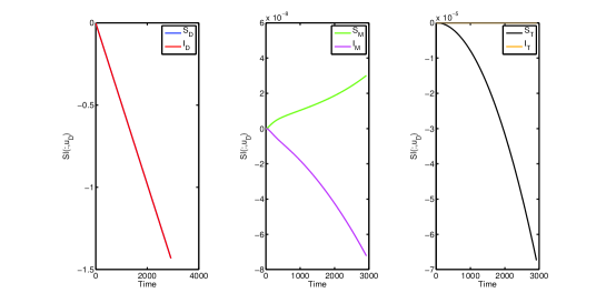
Figure 5: Population Dynamics (top) and Sensitivity indices w.r.t   $\mu_{D}$ for model (1). Parameters were chosen such that $R_{0}>1$. Initial values are same as in table 1.

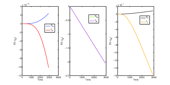
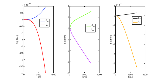
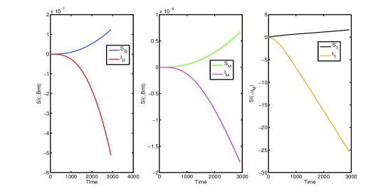
Figure 6: Sensitivity indices w.r.t   $\mu_{M}$ (top), $\beta_{TM}$ (middle), and $\beta_{MT}$ (bottom) for model (5). Parameters were chosen such that $R_{0}>1$. Initial values are same as in table 1.

5 Logistic Growth Modification

We now explore the effects of modeling the Deer population dynamics as logistic model. We consider this modification since large mammal density may be 1-2 orders of magnitudes lower than small mammal host [Kelker, 1947]. Deer-specific resource limitations may play an important role in the disease dynamics via the introduction of new susceptible Ticks.

$${}\quad\begin{cases}\dot{S_{D}}=\Lambda_{D}D\left(1-\frac{D}{K}\right)-\beta_{TD}\dfrac{I_{T}}{T}S_{D}-\mu_{D}S_{D}\vspace{1.5mm},\\ \dot{I_{D}}=\beta_{TD}\dfrac{I_{T}}{T}S_{D}-\mu_{D}I_{D}\vspace{1.5mm},\\ \dot{S_{M}}=\Lambda_{M}-\beta_{TM}\dfrac{I_{T}}{T}S_{M}-\mu_{M}S_{M}\vspace{1.5mm}\\ \dot{I_{M}}=\beta_{TM}\dfrac{I_{T}}{T}S_{M}-\mu_{M}I_{M}\vspace{1.5mm}\\ \dot{S_{T}}=\Lambda_{T}D-\beta_{MT}S_{T}\dfrac{I_{M}}{M}-\mu_{T}S_{T}\vspace{1.5mm}\\ \dot{I_{T}}=\beta_{MT}S_{T}\dfrac{I_{M}}{M}-\mu_{T}I_{T}\vspace{1.5mm}\\ \end{cases}$$ (5)

The modified model keeps all previously held assumptions, except $\Lambda_{D}$ now describes an intrinsic growth rate for the Deer population and $K$ which denotes carrying capacity.

5.1 Disease-free and endemic equilibria and their stability

Theorem 3.

If $\mathcal{R}_{0}<1$, then the disease free equilibrium, $E_{0}$, is locally asymptotically stable for the system (5). If $\mathcal{R}_{0}>1$, then $E_{0}$ is unstable. [den Driessche and Watmough, 2002]

The system (5) has a disease free equilibrium denoted by $E_{0}$, where

$$E_{0}=\left\{S_{D}\to\frac{K(\Lambda_{D}-\mu_{D})}{\Lambda_{D}},\text{I}_{D}\to 0,S_{M}\to\frac{\Lambda_{M}}{\mu_{M}},\text{I}_{M}\to 0,S_{T}\to\frac{K(\Lambda_{D}-\mu_{D})\Lambda_{T}}{\Lambda_{D}\mu_{T}},\text{I}_{T}\to 0\right\}$$

Thus, we require $\Lambda_{D}>\mu_{D}$ for existence. For stability, evaluating the Jacobian at the equilibria yields the following eigenvalues:

$$\lambda_{1,2,3,4}=\left(\begin{array}[]{c}-\mu_{D}\\ -\mu_{T}\\ -\mu_{M}\\ -\Lambda_{D}+\mu_{D}\\ \end{array}\right)$$

$$\lambda_{5,6}=-\frac{1}{2}\left(\mu_{M}+\mu_{T}\pm\sqrt{\mu_{M}^{2}-2\mu_{T}\mu_{M}+\mu_{T}^{2}+4\beta_{MT}\beta_{TM}}\right)$$

Notice that:

$$A =(\mu_{M}+\mu_{T})^{2}-\left(\mu_{M}^{2}-2\mu_{T}\mu_{M}+\mu_{T}^{2}+4\beta_{MT}\beta_{TM}\right)$$

$$=4(-\beta_{MT}\beta_{TM}+\mu_{T}\mu_{M})$$

Thus for stability, we additionally require:

$$\mathcal{R}_{0}=\sqrt{\frac{\beta_{MT}\beta_{TM}}{\mu_{T}\mu_{M}}}<1$$

Theorem 4.

The system (5) has a unique endemic equilibrium, $E^{*}=(S^{*}_{D},I^{*}_{D},S^{*}_{M},I^{*}_{M},S^{*}_{T},I^{*}_{T})$, iff $\mathcal{R}_{0}>1$. The endemic equilibrium $E^{*}$ is locally asymptotically stable whenever it exists.

The endemic equilibria of the model is the following:

$$S^{*}_{D}=\frac{(\Lambda_{D}-\mu_{D})(\mu_{T}+\beta_{MT})K\beta_{TM}\mu_{D}}{((\beta_{MT}\beta_{TM}-\mu_{T}\mu_{M})\beta_{TD}+\beta_{TM}\mu_{D}(\mu_{T}+\beta_{MT}))\Lambda_{D}}$$

$$I^{*}_{D}=\frac{(\Lambda_{D}-\mu_{D})(\beta_{MT}\beta_{TM}-\mu_{T}\mu_{M})K\beta_{TD}}{((\beta_{MT}\beta_{TM}-\mu_{T}\mu_{M})\beta_{TD}+\beta_{TM}\mu_{D}(\mu_{T}+\beta_{MT}))\Lambda_{D}}$$

$$S^{*}_{M}=\frac{\Lambda_{M}(\mu_{T}+\beta_{MT})}{\beta_{MT}(\mu_{M}+\beta_{TM})}$$

$$I^{*}_{M}=\frac{\Lambda_{M}(\beta_{MT}\beta_{TM}-\mu_{T}\mu_{M})}{\beta_{MT}\mu_{M}(\mu_{M}+\beta_{TM})}$$

$$S^{*}_{T}=\frac{\Lambda_{T}(\mu_{M}+\beta_{TM})(\Lambda_{D}-\mu_{D})K}{\beta_{TM}\Lambda_{D}(\mu_{T}+\beta_{MT})}$$

$$I^{*}_{T}=\frac{\Lambda_{T}(\beta_{MT}\beta_{TM}-\mu_{T}\mu_{M})(\Lambda_{D}-\mu_{D})K}{\beta_{TM}\Lambda_{D}\mu_{T}(\mu_{T}+\beta_{MT})}$$

To verify stability we examine the eigenvalues of the Jacobian matrix at the endemic equilibria:

$$\lambda_{1,2,3}=\left(\begin{array}[]{c}-\mu_{T}\\ -\mu_{M}\\ -\Lambda_{D}+\mu_{M}\\ \end{array}\right)$$

$$\lambda_{4}=-\frac{(\beta_{MT}\beta_{TM}-\mu_{T}\mu_{M})\beta_{TD}+\beta_{TM}\mu_{D}\mu_{T}+\mu_{D}\beta_{TM}\beta_{MT}}{\beta_{TM}(\mu_{T}+\beta_{MT})}$$

$$\lambda_{5,6}=-\left(A_{1}\pm\sqrt{A_{2}}\right)$$

Where:

$$A_{1}=\beta_{MT}^{2}\beta_{TM}-\beta_{TM}\mu_{T}^{2}+\beta_{MT}(-(\beta_{TM}+\mu_{M})^{2}-2\beta_{TM}\mu_{T})\\ A_{2}=-4(\beta_{TM}+\mu_{M})^{2}(\beta_{MT}+\mu_{M})^{2}(\beta_{MT}\beta_{TM}-\mu_{T}\mu_{M})+\beta_{MT}^{2}\beta_{TM}+\beta_{TM}\mu_{T}^{2}+\beta_{MT}((\beta_{TM}+\mu_{M})^{2}+2\beta_{TM}\mu_{T})^{2}$$

$\lambda_{4}$ is clearly negative whenever $\mathcal{R}_{0}>1$. Furthermore, simple calculations show that $\lambda_{5,6}$ are also negative since:

$$A_{1}^{2}-A_{2}=4(\mu_{M}+\beta_{TM})^{2}(\mu_{T}+\beta_{MT})^{2}(\beta_{MT}\beta_{TM}-\mu_{T}\mu_{M})>0$$

when

$$\mathcal{R}_{0}=\sqrt{\frac{\beta_{MT}\beta_{TM}}{\mu_{T}\mu_{M}}}>1$$

5.2 Forward Sensitivity Analysis

The Forward sensitivity equations for model (5) are identical to those for model (1). For instance, the equations w.r.t. $\beta_{TM}$ are:

$$\frac{\partial S_{D}}{\partial{\beta_{TM}}}=\Lambda_{D}\left(\frac{\partial S_{D}}{\partial{\beta_{TM}}}+\frac{\partial I_{D}}{\partial{\beta_{TM}}}\right)\left(1-\frac{2D}{K}\right)-\frac{\beta_{TD}}{T^{2}}\bigg{(}(I_{T}\frac{\partial S_{D}}{\partial{\beta_{TM}}}\ \frac{\partial I_{T}}{\partial{\beta_{TM}}})T-I_{T}S_{D}(\frac{\partial S_{T}}{\partial{\beta_{TM}}}+\frac{\partial I_{T}}{\partial{\beta_{TM}}})\bigg{)}-\beta_{TM}\frac{\partial S_{D}}{\partial{\beta_{TM}}}-S_{D}$$

$$\frac{\partial I_{D}}{\partial{\beta_{TM}}}=\frac{\beta_{TD}}{T^{2}}\bigg{(}(I_{T}\frac{\partial S_{D}}{\partial{\beta_{TM}}}+S_{D}\frac{\partial I_{T}}{\partial{\beta_{TM}}})T-I_{T}S_{D}(\frac{\partial S_{T}}{\partial{\beta_{TM}}}+\frac{\partial I_{T}}{\partial{\beta_{TM}}})\bigg{)}-\beta_{TM}\frac{\partial I_{D}}{\partial{\beta_{TM}}}$$

$$\frac{\partial S_{M}}{\partial{\beta_{TM}}}=-\frac{\beta_{TM}}{T^{2}}\bigg{(}(I_{T}\frac{\partial S_{M}}{\partial{\beta_{TM}}}+S_{M}\frac{\partial I_{T}}{\partial{\beta_{TM}}})T-I_{T}S_{M}(\frac{\partial S_{T}}{\partial{\beta_{TM}}}+\frac{\partial I_{T}}{\partial{\beta_{TM}}})\bigg{)}-\mu_{M}\frac{\partial S_{M}}{\partial{\beta_{TM}}}-S_{M}\frac{I_{T}}{T}$$

$$\frac{\partial I_{M}}{\partial{\beta_{TM}}}=\frac{\beta_{TM}}{T^{2}}\bigg{(}(I_{T}\frac{\partial S_{M}}{\partial{\beta_{TM}}}+S_{M}\frac{\partial I_{T}}{\partial{\beta_{TM}}})T-I_{T}S_{M}(\frac{\partial S_{T}}{\partial{\beta_{TM}}}+\frac{\partial I_{T}}{\partial{\beta_{TM}}})\bigg{)}-\mu_{M}\frac{\partial I_{M}}{\partial{\beta_{TM}}}+S_{M}\frac{I_{T}}{T}$$

$$\frac{\partial S_{T}}{\partial{\beta_{TM}}}=\Lambda_{T}\bigg{(}\frac{\partial S_{D}}{\partial{\beta_{TM}}}+\frac{\partial I_{D}}{\partial{\beta_{TM}}}\bigg{)}-\frac{\beta_{MT}}{M^{2}}\bigg{(}(S_{T}\frac{\partial I_{M}}{\partial{\beta_{TM}}}+I_{M}\frac{\partial S_{T}}{\partial{\beta_{TM}}})M-S_{T}I_{M}(\frac{\partial S_{M}}{\partial{\beta_{TM}}}+\frac{\partial I_{M}}{\partial{\beta_{TM}}})\bigg{)}-\mu_{T}\frac{\partial S_{T}}{\partial{\beta_{TM}}}$$

$$\frac{\partial I_{T}}{\partial{\beta_{TM}}}=\frac{\beta_{MT}}{M^{2}}\bigg{(}(S_{T}\frac{\partial I_{M}}{\partial{\beta_{TM}}}+I_{M}\frac{\partial S_{T}}{\partial{\beta_{TM}}})M-S_{T}I_{M}(\frac{\partial S_{M}}{\partial{\beta_{TM}}}+\frac{\partial I_{M}}{\partial{\beta_{TM}}})\bigg{)}-\mu_{T}\frac{\partial I_{T}}{\partial{\beta_{TM}}}$$

The results show some interesting contrasts with model (1). The sensitivity of the susceptible Deer population to $\mu_{D}$ rebounds once the population reaches carrying capacity, while the infected Deer class remains relatively more sensitive. The sensitivity of the infected mice class to $\mu_{D}$ is never positive (compared to model (1)) indicating that deer harvesting always decreases overall infection.

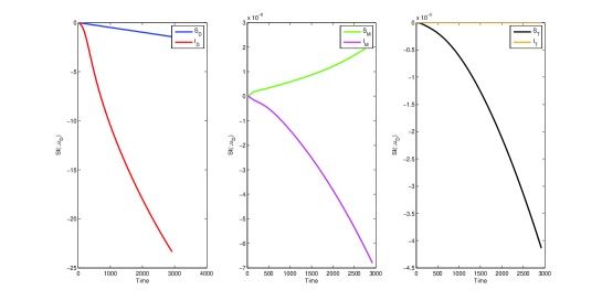
Figure 7: Population Dynamics (top) and Sensitivity indices w.r.t   $\mu_{D}$ for model (5). Parameters were chosen such that $R_{0}>1$. K = 5000, and initial values are same as in table 1.

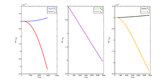
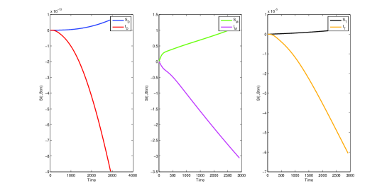
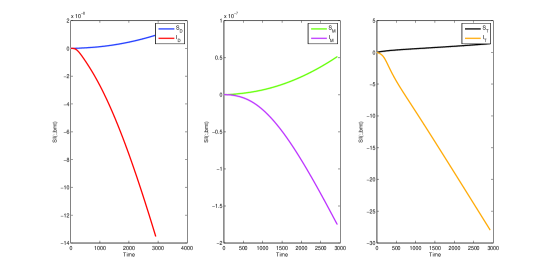
Figure 8: Sensitivity indices w.r.t   $\mu_{M}$ (top), $\beta_{TM}$ (middle), and $\beta_{MT}$ (bottom) for model (5). Parameters were chosen such that $R_{0}>1$. K = 5000, and initial values are same as in table 1.

6 Discussion

The rapid increase in Lyme disease cases in humans highlights the need to control the spread of infected black-legged ticks. We present a compartmental, SI model of the spread of Lyme disease for deer, tick and mice compartments in which the populations are grouped in susceptible and infected classes. The host, reservoir and vector dynamics in this particular model is crucial due to the life cycle of the tick. They reproduce mostly on deer, but get infected with the bacteria when feeding on mice during the nymphal stage. This implies that the birthrate of the ticks is dependent on the density of the deer. The parameters chosen to perform sensitivity analysis are the death rates of the reservoir host and the vector, as well as transmission rates between the two. The possibility of altering these parameters by introducing control methods in a real population of deer, mice and ticks prompted us to focus on said death rates and transmission rates. Analyzing the death rates of ticks, for example, would be the most effective but not realistic in terms of implementing policies. The dynamic sensitivity analysis of this model was performed to observe how the sensitivity changes over time when parameters relevant for control methods are perturbed.

The evolution of the susceptible and infected classes over a period of 3000 days indicates a pronounced increase in the numbers of susceptible mice which decreases after day 2000. This is mainly due to the values of the per capita death rate of the mice as well as the slow increase of the infected mice. The population of the deer remains relatively constant in number over the time interval of the simulation. Dynamic and static sensitivity analyses were performed on the model at the reproductive number and at the endemic equilibrium respectively. The static sensitivity of the reproductive number with respect to the death rates of the deer and mice yielded negative sensitivity values, which implies a reduction of the basic reproduction number. As $\mathcal{R}_{0}$ depends on transmission rates and death rates of mice and ticks, increasing the death rate of the deer or mice will cause this number to reduce, as $\mu_{M}$ is in the denominator of the expression. In the case of the deer, as we are reducing the reproductive host of the ticks, the population of ticks declines and this change is reflected in the decrease of the reproductive number [M. A. Diuk-Wasser and Piesman, 2006]. Decreasing the transmission rates between mice and ticks produces a negative sensitivity for the $R_{0}$. This can be intuitively seen as the transmission rates are located in the denominator of $R_{0}$; it follows that any increase in the transmission rates would result in a decrease in $R_{0}$. At the endemic equilibrium, the death rate of the deer had a larger impact on the infected tick population compared to the effect it had on the infected mice population. The sensitivity index at the endemic equilibrium of the infected mice population with respect to the death rate of the deer was zero; in spite of this, we cannot conclude that there is no effect but rather that it is a secondary effect that is not reflected in this first order approximation. Decreasing the population of mice has a large impact on the infected tick population, as the reservoir host of the bacteria is reduced thus infecting less ticks. It had a small negative impact on the infected deer population, which was an indirect consequence of reducing the infected tick population.

The dynamical sensitivity analysis with respect to deer death rate reflected a direct negative impact on the infected deer population. The population of susceptible ticks decreases as the host on which they reproduce is culled. As a consequence there is a small increase in the susceptible mice population and a decline in infected mice. Lowering the number of deer reduces the population of ticks quite efficiently. However, the increase of infected mice is a problem because the number of infected ticks will start increasing over time as the susceptible mice decrease. Decreasing the numbers of both susceptible and infected mice constantly in an interval of time impacts the tick population directly. The effect is most pronounced in the infected class which experiences a dramatic reduction. Infected mice decline, causing an important reduction in the infected tick population, which is a direct consequence of the transmission rate of the disease from mice to ticks [E. M. Bosler and Benach, 1984]. Additionally, as mice act as the reservoir host for Lyme disease [Buskirk and Ostfeld, 1995], when the number of infected mice decreases, so does the infected tick population. Although the tick population does not drastically decrease, the importance of increasing the mouse death rate is that we are reducing the pool of infectious hosts that spread the disease. Increasing the death rate of the mice has some benefits over increasing the death rate of the deer, in spite of the small impact on the infected tick population. Ticks have preferred hosts, however their survival is a direct result of their adaptability [Ostfeld, 2010]. Thus, if there is a reduction of the deer, the reduced tick population could potentially switch hosts, increasing the number of infected mice [Barbour and Fish, 1993].

Altering the transmission rates is also a possibility when it comes to trying to control Lyme disease. The transmission rates between mice and ticks depend on the probability of contact and biting rate. The strategy used by the CDC in a study currently underway in Connecticut was to place bait boxes with food for mice. These boxes also include a wick with the pesticide, fipronil, which kills tick on the mice without harming the mammal [CDC,]. In the dynamic sensitivity analysis performed with respect to the transmission rates we obtained different sensitivities indices depending on whether the transmission rate was from tick to deer or vice versa. When decreasing $\beta_{MT}$, the transmission rate from mice to tick, there is a considerable decrease in the infected tick population, but a very small impact on the infected mice population which is a secondary effect. Decreasing the transmission rate from tick to mice impacts the infected mice population negatively, but has a small effect in the decrease of infected tick populations.

6.1 Future Work

This model has the limitation of not including the life cycle of I. scapularis and the different hosts that it inhabits in each stage of its life. This would be relevant to introduce control measures in a specific host at a particular life stage of the tick to prevent the tick from acquiring the bacteria (rodent control) or reducing the total population of ticks (large mammal control). Another possible issue with the model is that our control measures consist of modifying death rates constantly over time; this is not realistic in the sense that controlling deer would be done once a year, during the hunting season, which is a yearly occurrence in a very short amount of time. For future work, we can consider introducing a harvesting term on the deer that reflects the hunting season more accurately and/or introducing the different life stages of the tick. We would also like to introduce a two-patch model that would incorporate migration, geographical restrictions, and variable harvesting restrictions per population. Including seasonality into the model would also be an interesting avenue for future study to increase accuracy. Additionally, we would like to calculate the total sensitivity of our populations as opposed to the instantaneous dynamic sensitivity. For example, from the functional $J(I_{D})=\int^{T}_{t=0}\frac{dI_{D}}{dt}\,dt$, we would use the adjoint method to determine the sensitivity of the total $I_{D}$ population.

7 Appendix

Table 3: Sources of the variables in the modeling framework

Parameter	Source
$D$	[Roseberry and Woolf, 1998]
$T$	[M. A. Diuk-Wasser and Piesman, 2006]
$S_{T}$	[M. A. Diuk-Wasser and Piesman, 2006]
$I_{T}$	[M. A. Diuk-Wasser and Piesman, 2006]
$\Lambda_{D}$	[Kelker, 1947]
$\Lambda_{M}$	[Fahrig and Merriam, 1985][Jacquot and Vessey, 1998]
$\Lambda_{T}$	[T. Levi and Wilmers, 2012]
$\beta_{TD}$	[T. Levi and Wilmers, 2012]
$\beta_{TM}$	[T. Levi and Wilmers, 2012]
$\beta_{MT}$	[T. Levi and Wilmers, 2012]
$\mu_{D}$	[M. Nelson, 1986]
$\mu_{M}$	[Fahrig and Merriam, 1985][Ruan et al., 1999]
$\mu_{T}$	[T. Levi and Wilmers, 2012]

References

- [A. C. Steere and Malawista, 1983] A. C. Steere, G. J. Hutchinson, D. W. R. L. H. S.-J. E. C. E. T. D. and Malawista, S. E. (1983). Treatment of the early manifestations of lyme disease. Annals of Internal Medicine, 99(1):22–26.
- [Arriola and Hyman, 2009] Arriola, L. and Hyman, J. M. (2009). Sensitivity analysis for uncertainty quantification in mathematical models. In Mathematical and Statistical Estimation Approaches in Epidemiology, pages 195–247. Springer.
- [Barbour and Fish, 1993] Barbour, A. G. and Fish, D. (1993). The biological and social phenomenon of lyme disease. SCIENCE-NEW YORK THEN WASHINGTON-, 260:1610–1610.
- [Buskirk and Ostfeld, 1995] Buskirk, J. V. and Ostfeld, R. S. (1995). Controlling lyme disease by modifying the density and species composition of tick hosts. Ecological Applications, 5(4):1133–1140.
- [CDC, ] CDC. Lyme disease data.
- [den Driessche and Watmough, 2002] den Driessche, P. V. and Watmough, J. (2002). Reproduction numbers and sub-threshold endemic equilibria for compartmental models of disease transmission. Mathematical biosciences, 180(1):29–48.
- [E. M. Bosler and Benach, 1984] E. M. Bosler, B. G. Ormiston, J. L. C. J. P. H. and Benach, J. L. (1984). Prevalence of the lyme disease spirochete in populations of white-tailed deer and white-footed mice. The Yale journal of biology and medicine, 57(4):651.