Chapter 1 introduction

Thirty years of active research in Pulsars have made it abundantly clear that these objects are veritable laboratories for testing out theories for exotic physics stretching far beyond the limits of present day terrestrial experiments. Indeed, the 1967 discovery of the first pulsar by Hewish and his group in Cambridge has been one of the major events in recent astronomy [Hewish et al. (1968]. Pulsars, characterized by the regular pulses of radiation observed to be coming from them, are actually strongly magnetized neutron stars rotating very rapidly. The concept of neutron stars, of course, has been around for about thirty years before this discovery, almost from the day the neutron was detected for the first time. It is said that the day the news of the discovery of neutrons reached Landau, he hypothesized on the possible existence of stars made up entirely of neutrons. Barely two years after this, ?) in their seminal paper propounded the theory of the possible birth of neutron stars in the most violent and spectacular event of stellar death, that of a supernova explosion.

There has always been a great interest in the ultimate fate of the stars. Before the advent of Fermi-Dirac statistics, it was inconceivable as to how a star could escape the final collapse at the hands of gravity when it exhausts its nuclear fuel - a view expounded by Sir Arthur Eddington. But the work of ?) proved conclusively that the final gravitational collapse could be halted when the stellar material becomes Fermi-degenerate due to extreme compression so that the degeneracy pressure is sufficient to withhold gravity. In this work the case of electron-degeneracy and the end state of stars that we know of as white dwarfs has been discussed. Soon afterwards the companion of Sirius was identified as a white dwarf which vindicated the existence of such degenerate end stages of stars. The logical extension of Chandrasekhar’s argument is, of course, the state when the neutrons become degenerate. And that is the state found in neutron stars.

Even before the discovery of pulsars, ?) suggested that the Crab Nebula must be powered by a rotating neutron star. The Crab Nebula is the remnant of the supernova of A.D. 1054, recorded by the Chinese. The later identification of the Crab Pulsar with the neutron star associated with the supernova gave the first direct proof of Baade & Zwicky’s hypothesis. Lately, the attention has been focussed on the most spectacular supernova of recent times, SN1987A, a supernova that went off in the Large Magellanic Cloud, a small companion galaxy of the Milky Way, in February 1987. But even after a decade of intense search the neutron star that is supposed to be there has remained elusive. This, in all probability, means a modification of the theory of neutron star formation in supernovae. Of course, supernovae may not be the only way of neutron star formation. Recently, particularly in connection with the possible ways of millisecond pulsar formation, the theory of accretion-induced collapse of a white dwarf into a neutron star has been advocated. Even if that does happen in certain systems, supernovae would still most likely be the major route through which the neutron stars are born. As a star of main-sequence mass $\raisebox{-1.29167pt}{\mbox{$\stackrel{{\scriptstyle>}}{{{}_{\sim}}}\,$}}8\mbox{{\rm M}${}_{\odot}$}$ explodes at the end of its life, it throws away most of its mass and the object that is left behind is a neutron star of mass of about $\sim 1.4~{}\mbox{{\rm M}${}_{\odot}$}$ with a radius of ten kilometers. Evidently the formation of this ultra-compact object is accompanied by a release of a tremendous amount of energy ($\sim 10^{53}$ erg) equal to the binding energy of it. And this is the energy that powers the fantastic fireworks of a supernova.

The initial interest in neutron stars, surprisingly, arose due to the discovery of certain intense radio emitters. The large values of red-shift associated with these objects made one think that these could be neutron stars producing highly red-shifted radiation due to the large value of their surface gravity. That idea died its natural death when quasars were discovered. Then in 1967 pulsars were discovered almost serendipitously, by Jocelyn Bell, a graduate student working with Anthony Hewish on interplanetary scintillation [Hewish et al. (1968]. Understandably, the first signals from the neutron star, due to their extreme regular periodicity, were suspected to have been signatures of the ’little green men’. But all such highly speculative theories and their more sober counterparts quickly settled to an identification of these objects as neutron stars [Gold (1968, Gold (1969]. The signals were understood to have originated due to the fast rotation of the neutron stars possessing very large magnetic fields (canonical value of the field being B $\sim 10^{12}$ Gauss). Extremely compact objects were required to explain the rapidity of the pulses ($P\sim s$) and the obvious candidates were the neutron stars and the white dwarfs. Discovery of fast pulsars like Crab and Vela (with rotation periods of 33 and 89 ms respectively) excluded the possibility of these being white dwarfs (as they would not be gravitationally stable at such high rates of rotation) and the identification of pulsars with neutron stars was conclusively established [Gold (1968, Gold (1969, Gunn & Ostriker (1969, Pacini (1968].

Pulsars are characterized by their pulsed emission and the precise periodicity of these pulses, though the shape and the amplitude of the pulse profiles vary widely. The mechanism of the radio emission still remains one of the important unsolved problems of pulsar physics, though the basic ideas were laid down quite early on by ?). In this model of magnetic dipole pulsar emission is derived from the kinetic energy of a rotating neutron star. It is assumed that a neutron star rotates uniformly in vacuum at a frequent $\omega$ and has a dipole moment m at an angle $\theta$ to the axis of rotation. The dipole field at the magnetic pole of the star, $B_{p}$, is related to m by

$$|{\bf m}|=\frac{1}{2}B_{p}R^{3},$$ (1.1)

where $R$ is the radius of the star. This oblique rotator configuration has a time-varying dipole moment as seen from infinity and therefore radiates energy at a rate

$$\dot{E} = -\frac{2}{3c^{3}}|\ddot{\bf m}|^{2}$$ (1.2)

$$= -\frac{1}{6c^{3}}B_{p}^{2}R^{6}\omega^{4}\sin^{2}\theta$$

This energy carried away changes the kinetic energy producing a slow-down torque on the star given by

$$N=I\dot{\omega},$$ (1.3)

where $I$ is the moment of inertia of the star. Using equation [1.2] and [1.3] one obtains an estimate of the magnetic field in terms of the period and the rate of change of the period of the star, which are measurable with high accuracy from the timing of the arriving pulses. Thus, the magnetic field is given by the expression [Manchester & Taylor (1977]

$$B\sim(\frac{3Ic^{3}P\dot{P}}{8\pi^{2}R^{6}})^{1/2},$$

where, $P,\dot{P}$ are the period and the period derivative, $I$ is the moment of inertia and $R$ is the radius of the star. There are problems with this simple model. Firstly, as far as the emission is concerned, this mechanism does not work in case of an aligned rotator. Refined theories dealing with the problem of emission for an aligned rotator have come into existence since then. And this simple estimate of the magnetic field provides a measure of the dipole component only, without any handle on the total field. Yet, this is still the most widely used and in most cases the only means of estimating the magnetic field. There have been a few direct measurements of the field, like that from the cyclotron line-strength of Her X-1, which gave the field strength of this neutron star to be $\sim 4-6\times 10^{12}$ Gauss [Truemper et al. (1978]. But the scope of such direct measurement is limited only to the case of X-ray binaries. For radio pulsars no method for a direct measurement of the field exists.

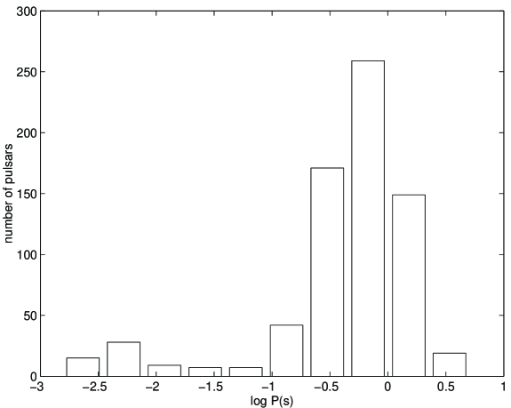
Figure 1.1: Histogram showing the period distribution of the radio pulsars.

With the discovery of a new variety of pulsar by Backer et al. (?) another horizon in the pulsar research opened up. From now on the radio pulsars were divided into two distinct classes with very different physical characteristics. The new variety were named millisecond pulsars as these have very small rotation periods, in the range of milliseconds. The first one observed, PSR1937+21, had a period of 1.6 ms. Also they were found to have extremely short (compared to the earlier-observed normal pulsars) magnetic fields in the range of $10^{8}-10^{9}$ Gauss. In all some seven hundred pulsars have been observed to date. Figure [1.1] shows a histogram for the periods of all these pulsars. The period distribution is clearly bimodal, with most of the occupants of the peak at short periods being millisecond pulsars. One must admit here that the definition of millisecond pulsars is somewhat ad hoc, defined as the ones with spin periods less than $20ms$. Still the division serves quite well due to the fact that these two sets, as far as present understanding goes, do have very different past histories. We make a crude comparison of these two classes of pulsars here in order to highlight the differences.

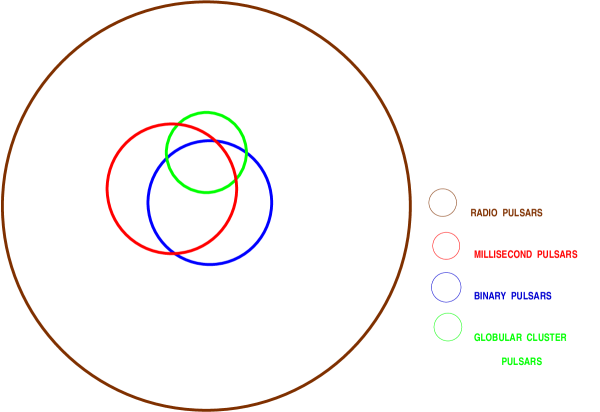
Figure 1.2: A schematic description of how the various special types of radio pulsars overlap with each other.

properties	normal pulsars	millisecond pulsars
spin period	$P\raisebox{-1.29167pt}{\mbox{$\stackrel{{\scriptstyle>}}{{{}_{\sim}}}\,$}}20$ ms	$P\raisebox{-1.29167pt}{\mbox{$\stackrel{{\scriptstyle<}}{{{}_{\sim}}}\,$}}20$ ms
magnetic field	$10^{11}-10^{13}$ Gauss	$10^{8}-10^{9}$ Gauss
age	$\raisebox{-1.29167pt}{\mbox{$\stackrel{{\scriptstyle>}}{{{}_{\sim}}}\,$}}10^{6}-10^{7}$ yrs	$\sim 10^{9}$ yrs
binarity	mostly isolated	mostly in binaries

The most striking difference is, of course, the fact that whereas the normal pulsars are mostly isolated, some 90% of the disk population and about 50% of the Globular Cluster population of the millisecond pulsars are in binaries. The age determination of some of the millisecond pulsars are possible also due to that fact. From the surface temperature of the white dwarf companion it has been possible to put a lower limit to the age of a few millisecond pulsars which lies in the range of $10^{9}$ years [Callanan et al. (1989, Kulkarni, Djorgovski, & Klemola (1991]. On the other hand, in the case of normal pulsars it is basically the spin-down age estimated from the rate of change of the period which turn out to be a few million years at most. To emphasize the remarkable binary-millisecond pulsar association we draw here a Venn-diagram in figure [1.2] showing the nature of the pulsars, their binary association and the population (disk or globular cluster) to which they belong.

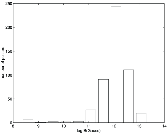
Figure 1.3: Histogram showing the distribution of the magnetic field in solitary radio pulsars.

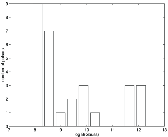
Figure 1.4: Histogram showing the distribution of the magnetic field in binary radio pulsars.

It has been observed that, in general, the binary pulsars have lower fields than the isolated pulsars. In figures [1.3] and [1.4] we have plotted the histograms of the field strengths of in these two categories separately.This fact was evident even in the first binary pulsar to be discovered, the famous PSR1913+16 discovered by ?). It was ?) who suggested for the first time a connection between the decay of the magnetic field in a neutron star and its binary association. ?) provided observational support to this idea. In the early eighties the idea of recycled pulsars was forwarded in this connection [Srinivasan & van den Heuvel (1982, Radhakrishnan & Srinivasan (1982, Alpar et al. (1982]. According to this scenario an otherwise normal pulsar, at the end of its normal lifetime, could be resurrected with a reduced magnetic field and a spun-up period if it is processed in a binary. One of the problems faced by the theory of recycled pulsars is that of explaining the isolated low-field and millisecond pulsars. ?) suggested that the companion could perhaps be ablated by the intense radiation falling on it from the pulsar. Soon afterwards PSR1957+20 (another 1.6 ms pulsar) was caught in the act of vaporising its companion [Fruchter, Stinebring, & Taylor (1988]. So that immediately confirmed this conjecture, although later on doubts have been raised regarding the efficacy of this method to completely destroy the companion. Yet, the connection between a reduction of the field strength and a binary history has remained well endorsed by observations. Though the theory of ‘recycling’ has its problems, to date this has been the most successful in explaining the population of the low-field and millisecond pulsars by integrating them with the class of normal pulsars through their binary history.

In order to develop a proper theory of the evolution of the magnetic field it is essential to understand the nature of the internal current configuration supporting the observed field. This also requires an accurate knowledge of the internal structure of the neutron stars which determines the long-term behaviour of the embedded current loops and hence the time-evolution of the magnetic field. Roughly, the neutron star has two physically different regions - the crust and the core. The crust is the outer shell, about a kilometer thick, which is a crystalline solid made up of neutron rich nuclei. In this region the density changes by some eight orders of magnitude, going from $10^{6}~{}{\rm g}\,{\rm cm}^{-3}$ at the very surface, to $10^{14.5}~{}{\rm g}\,{\rm cm}^{-3}$ at the boundary of the crust and the core [Pandharipande, Pines, & Smith (1976]. Underneath this crust lies the region with an average density of nuclear density or more, which is believed to have superfluid neutrons along with superconducting protons and extremely relativistic, Fermi degenerate electrons [Lattimer (1992, Pines & Alpar (1992]. There is a lot of controversy about the exact composition of the core, opinions ranging from normal n-p-e plasma to exotic quark-condensates [Hanawa (1992, Lattimer et al. (1991, Pethick (1992, Prakash (1994, Tatsumi & Muto (1992], but the above-mentioned picture is what is generally accepted at present.

Regarding the generation of the magnetic field in the neutron stars, there are two possibilities. The field could be a fossil field. The original magnetic field of the progenitor of the neutron star could be enhanced to large values by flux conservation during compactification of the large star to neutron star dimensions. As one believes the core to become superfluid soon after formation and in particular the protons form a type II superconductor, the field would be supported by the proton superconducting flux tubes in this case. But there are problems with this scenario. Firstly, there are no good measurements for the core field of the massive stars, so it is not certain whether the field strength required to enhance it to the pulsars field values really obtain in the progenitor core. On the other hand, in an extremely violent process like a supernova explosion, whether an adiabatic process like flux conservation would hold good is not clearly understood. The other possibility is that of the generation of the field after the birth of the neutron star. ?) pointed out that it is possible to generate a field in the crust of a cooling neutron star due to thermo-magnetic instabilities as the heat flows in presence of a seed field. This mechanism, again, suffers from the fact that a seed field of the order of $10^{8}$ Gauss is required in order to produce the canonical field values that are observed in neutron stars. Though none of the theories are free from hitches, for want of better alternatives, these are accepted as the best possibilities for the origin of the field in neutron stars.

It is, of course, obvious that the evolution of the field would itself depend on the generation mechanism, which determines the underlying configuration of currents. Initially, observational data appeared to indicate that the pulsar magnetic fields decay with a time constant of $\sim 10^{6}$ years [Gunn & Ostriker (1970, Lyne, Anderson, & Salter (1982] On the other hand, it was shown by ?) that given the state of matter in a neutron star the electrical conductivity is expected to be extremely high and the ohmic dissipation time-scale should be larger than the Hubble time. It was borne out by some recent statistical work [Bhattacharya et al. (1992, Hartman et al. (1997], where they showed that the magnetic field of the isolated pulsars indeed do not show any significant decay. An investigation of the association of the field decay and a binary history therefore becomes extremely pertinent. In the past few years a considerable amount of effort has been spent in trying to find the answer to this question (for details see [Bhattacharya & Srinivasan (1995] and references therein). The basic understanding in this regard could be divided into two classes. The underlying physics of the field evolution in a binary is that of the ohmic dissipation of the current loops in the accretion-heated crust. Therefore, for the believers in crustal field, the current dissipates due to an increase in temperature as mass is accreted by the neutron star from its companion in the course of binary evolution. When one assumes an initial core field configuration, a phase of spin-down driven flux-expulsion is necessary prior to the phase of the ohmic dissipation in the crust. Both these ideas have been explored in detail by a multitude of researchers (for a review see [Bhattacharya (1995b]) yet by no means have all the questions been answered.

Therefore, fifteen years after the discovery of the millisecond pulsars there still remains a lot of uncertainties regarding their possible past history. On a broader perspective the scenarios for both the generation and the evolution of magnetic fields of neutron stars lack a consensus. A coherent theoretical picture is yet to emerge. In such a situation, the observational data is the only guide. In this thesis, therefore, we have tried to address a few questions related to the evolution of the magnetic field of neutron stars that are members of binary systems. We try to make connection with the overall picture of the field evolution as indicated by observational data. In particular we look into the problem of the generation of millisecond pulsar from particular kind of binary systems. To this end we have looked at four related problems as described below :

• the effect of diamagnetic screening on the final field of a neutron star accreting material from its binary companion;

• evolution of magnetic flux located in the crust of an accreting neutron star;

• application of the above-mentioned model to real systems and a comparison with observations;

• an investigation into the consequences of magnetic flux being initially located in the core of the star and its observational implications.

Here then is a brief resume of the problems mentioned above.

1. The effect of diamagnetic screening - The basic idea is that the magnetic field is screened due to the stream of the accreting material that arrives at the polar cap, being channeled by the strong magnetic field of the star. A screening of the external dipole field, in this case, is achieved by the production of horizontal components at the cost of poloidal ones. If fluid-interchange instabilities are ignored then the field lines are frozen to the material (since the flow time-scales are very much smaller than the diffusive time-scales) and as the accreted material spreads over the surface it drags the field lines along. The field lines would then reconnect on the equatorial plane and get buried. Before this field can diffuse out more matter will come and spread on top of it, and push the field to even deeper regions. Finally the field may even reach the superconducting core from where it will not diffuse out. But whether such burial is at all possible depends on the relative magnitude of the time-scales of flow, diffusion and interchange instability. This question has already been addressed before, and the calculations made by us re-assert the fact that the fluid-interchange time-scales are too small for the burial of the field to be effective since any stretching of the field lines is quickly restored over this overturn time-scale. Therefore the cause of the low field observed in some neutron stars in X-ray binaries or in millisecond pulsars can not be due to a simple screening of their magnetic field by the accreted matter.

2. Evolution of a crustal magnetic flux under accretion - This investigation is carried out assuming the underlying currents, supporting the observed field, to be entirely confined to the crust of the neutron star to start with. The main mechanism responsible for the field decay here is the ohmic dissipation of the current loops in the accretion-heated crust. The evolution is investigated for a wide range of values of the relevant physical parameters, such as the rate of accretion, the depth of current carrying layers etc. We find that within a reasonable range of parameter values final fields in the correct range for millisecond pulsars are produced. A most important feature has been seen to arise due to the inward material movement of the crustal layers because of accreted overburden. The current loops reach the region of very high conductivity in the deeper and denser regions of the star by such material movement and this puts a stop to further field decay. This freezing in behaviour that comes naturally out of the input physics, is very important in explaining the limiting field values observed in binary and millisecond pulsars. Therefore, within the limits of uncertainty this model, besides providing for an effective mechanism for field reduction by the right order of magnitude, also gives an explanation for the lower bound of the field observed in millisecond pulsars.

3. Comparison with observations - Here we investigate the evolution of the magnetic field of neutron stars in its entirety – in case of the isolated pulsars as well as in different kinds of binary systems, assuming the field to be originally confined in the crust. A comparison of our results for the field evolution in isolated neutron stars with observational data helps us constrain the physical parameters of the crust. We also model the full evolution of a neutron star in a binary system through several stages of interaction. Initially there is no interaction between the components of the binary and the evolution of the neutron star is similar to that of an isolated one. It then interacts with the stellar wind of the companion and finally a phase of heavy mass transfer ensues through Roche-lobe overflow. We model the field evolution through all these stages and compare the resulting final field strength with that observed in neutron stars in various types of binary systems. One of the interesting aspects of our result is a positive correlation between the rate of accretion and the final field strength. Recently there has been observational indications for such a correlation. Our results also match with the overall picture of the field evolution in neutron stars. In particular, the generation of millisecond pulsars from low-mass binaries arises as a natural consequence of the general framework.

4. Lastly, we look at the outcome of spindown-induced expulsion of magnetic flux originally confined to the core, in which case the expelled flux undergoes ohmic decay. We model this decay of the expelled flux. Once again we look into the nature of field evolution – both for neutron stars that are isolated and are members of binary systems. This scenario of field evolution could also explain the observed field strength of neutron stars but only if the crustal lattice contains a large amount of impurity. At present both the scenarios (assuming an original crustal field and an expelled flux) appear to be consistent with the observations though they require rather different assumptions regarding the state of the matter in the crusts of the neutron stars. Also, the detailed predictions in the two scenarios are different. Therefore future observations, able to pin down these details, should distinguish between the two models. On the other hand, with an unambiguous determination of the state of the matter in the neutron star crust, at some future date, it will again be possible to arrive at a definitive conclusion regarding the model of field evolution that actually prevails in neutron stars.

Improved observational techniques have produced a wealth of data in the recent past which requires an accurate and detailed understanding of pulsar physics. Unfortunately, the regime in which the physical theories are lacking are precisely the regimes in which the neutron stars are the only available systems. And the data, though enormous, still remain inadequate for answering such questions unambiguously. The handicap is many-faceted, like the uncertainty in the form of a nucleon-nucleon interaction potential or the inadequacy of the quantum many body techniques to handle the nuclear density systems. Even though the basic picture of field reduction via ohmic dissipation is on secure grounds there are still many uncertainties, for example due to uncertainties in :

• the crustal structure, in particular regarding the exact forms of the nuclei,

• the transport properties arising due to a lack of proper knowledge of the impurity concentration or the dislocations that exist in the crust,

• the change in the composition due to accretion, since the newly-formed accreted crust do not contain cold-catalysed matter like the original crust, or

• the thermal behaviour in both isolated and accreting neutron star.

As for the generation of the millisecond pulsars, quite apart from the birthrate problem, all the model calculations also suffer from uncertainties in the binary evolution.

If the physics of these are understood a lot of accepted wisdom may change. Refined many-body calculations of proton superconductivity has already cast doubts on the magnetic field being supported by the fluxoids threading the core [Ainsworth, Wambach, & Pines (1989]. Therefore to understand the basic problems at least within the standard premises one needs to have a second look at the problems incorporating all the new refinements that have been coming in. That seems to be the next logical step. On a different level, new and exotic physics is making inroads like the Strange stars being put forward as possible pulsar candidates [Cheng & Dai (1997]. Those probably would start the new era of pulsar research.

This thesis has been organized as follows. In chapter 2, we review the basics of neutron star physics, aspects that we have needed for our calculations. Chapter 3 discusses the standard scenario for the generation and evolution of neutron star magnetic fields. In chapters 4 to 7 we describe the details of the four problems that have been worked on. Finally in chapter 8 we have made our conclusions along with a discussion of the uncertainties inherent in these investigations and the possible future directions of work along these lines.

Chapter 2 microphysics of neutron stars

2.1 equation of state of dense matter

The conditions in the interior of Neutron Stars are more extreme than any encountered terrestrially. The gravitational pressure is supported mainly by the pressure of the repulsive interaction of the nucleons. To a first approximation a neutron star is like a giant nucleus made of $10^{57}$ nucleons (mostly neutrons) with an average baryon density close to the nuclear density. The star also has a solid crust roughly one kilometer thick, compositionally similar to terrestrial crystalline solids with highly neutron-rich nuclei. The core beneath the crust is essentially a sea of neutrons with a mere ten percent sprinkling of protons and an equal number of electrons to maintain charge neutrality. Besides having an average density of about $\sim 10^{15}~{}{\rm g}\,{\rm cm}^{-3}$ a neutron star also has a huge neutron excess. When a neutron star forms in a supernova explosion the temperature attained is higher than the characteristic temperatures of all the equilibrating chemical reactions. Consequently, all of the neutron star material is $\beta$-equilibrated where most of the protons have been converted to neutrons due to enhanced inverse $\beta$-decay in a dense environment. As the electron Fermi sea is filled up the reverse process, i.e., the decay of a neutron to a proton, an electron and an anti-neutrino, is progressively blocked resulting in the neutron excess.

Except near the surface the neutron star behaves like an effective zero-temperature system, the actual temperature ($\sim 10^{6}$K or less in the crust and $\raisebox{-1.29167pt}{\mbox{$\stackrel{{\scriptstyle<}}{{{}_{\sim}}}\,$}}10^{8}$K in the core after about $10^{4}$ years) being much smaller than the characteristic temperatures (the Fermi temperature of the electrons or the neutrons or the energy of the nucleon-nucleon interaction). Therefore almost whole of the star can be described as a degenerate, free Fermi system (electrons being the dominant component near the surface and neutrons in the interior). We shall not discuss here the superfluid states of neutrons or protons believed to exist in the core. Density-wise the neutron star has three characteristically different regions. The thin outer crust with densities ranging from $10^{6}~{}{\rm g}\,{\rm cm}^{-3}$ at the surface to $4.0\times 10^{11}~{}{\rm g}\,{\rm cm}^{-3}$ (neutron drip density) at which free neutrons start dripping out of the nuclei. Next is the inner crust with densities in-between the neutron-drip density and the nuclear density ($2.8\times 10^{14}~{}{\rm g}\,{\rm cm}^{-3}$). Beyond the nuclear density the nuclei dissolve to produce a soup of nucleons.

2.1.1 outer crust : $7.86~{}{\rm g}\,{\rm cm}^{-3}<\rho<4.0\times 10^{11}~{}{\rm g}\,{\rm cm}^{-3}$

This is the best understood density regime of all. The pressure is primarily due to that of the degenerate electrons, charge neutrality being maintained by an ionic crystal. For $\rho\raisebox{-1.29167pt}{\mbox{$\stackrel{{\scriptstyle>}}{{{}_{\sim}}}\,$}}10^{6}~{}{\rm g}\,{\rm cm}^{-3}$ the electrons become relativistic. As density increases beyond this value the electron Fermi energy approaches the MeV range where it becomes energetically favourable for the protons to undergo inverse $\beta$-decay and convert themselves to neutrons giving rise to the neutron-rich nuclei in the crust. The equilibrium nuclide for a given density is obtained by minimizing the free energy of the system with respect to a particular combination of ($Z,A$) keeping the baryon number density constant. The first such calculation was done by ?), reproduced here in table [2.1], based on Bethe-Weizs̈acker semi-empirical mass formula with parameters obtained from fits to laboratory nuclei. Recently, ?) have redone these calculations using more refined methods, though their results do not differ very much from the earlier ones. Among the factors important in deciding the equilibrium nuclide at a given density are the neutron and proton (dominant just below the neutron drip) shell effects and the strength of the spin-orbit interaction which depends on the three and higher body nucleon-nucleon interactions (defining the energy of the individual nuclei).

TABLE 2.1
DATA FROM BAYM, PETHICK AND SUTHERLAND (1971)
mass density	baryon number density	mass number	atomic number
		of equilibrium nuclide	of equilibrium nuclide
$\rho$ (${\rm g}\,{\rm cm}^{-3}$)	$n_{b}$ (cm-3)	$Z$	$A$
7.86E0	4.73E24	26	56
7.90E0	4.76E24	26	56
8.15E0	4.91E24	26	56
1.16E01	6.99E24	26	56
1.64E01	9.90E24	26	56
4.51E01	2.72E25	26	56
2.12E02	1.27E26	26	56
1.150E03	6.93E26	26	56
1.044E04	6.295E27	26	56
2.622E04	1.581E28	26	56
6.587E04	3.972E28	26	56
1.654E05	9.976E28	26	56
4.156E05	2.506E29	26	56
1.044E06	6.294E29	26	56
2.622E06	1.581E30	26	56
6.588E06	3.972E30	26	56
8.293E06	5.000E30	28	62
1.655E07	9.976E30	28	62
3.302E07	1.990E31	28	62
6.589E07	3.972E31	28	62
1.315E08	7.924E31	28	62
2.624E08	1.581E32	28	62
3.304E08	1.990E32	28	64
5.237E08	3.155E32	28	64
8.301E08	5.000E32	28	64
1.045E09	6.294E32	28	64
1.316E09	7.924E32	34	84
1.657E09	9.976E32	34	84
2.626E09	1.581E33	34	84
4.164E09	2.506E33	34	84
6.601E09	3.972E33	34	84
8.312E09	5.000E33	32	82
1.046E10	6.294E33	32	82
1.318E10	7.924E33	32	82
1.659E10	9.976E33	32	82
2.090E10	1.256E34	32	82
2.631E10	1.581E34	30	80
3.313E10	1.990E34	30	80
4.172E10	2.506E34	30	80
5.254E10	3.155E34	28	78

TABLE 2.1 (continuted)
DATA FROM BAYM, PETHICK AND SUTHERLAND (1971)
mass density	baryon number density	mass number	atomic number
		of equilibrium nuclide	of equilibrium nuclide
$\rho$ (${\rm g}\,{\rm cm}^{-3}$)	$n_{b}$ (cm-3)	$Z$	$A$
6.617E10	3.972E34	28	78
8.332E10	5.000E34	28	78
1.049E11	6.294E34	28	78
1.322E11	7.924E34	28	78
1.664E11	9.976E34	26	76
1.844E11	1.105E35	42	124
2.096E11	1.256E35	40	122
2.640E11	1.581E35	40	122
3.325E11	1.990E35	38	120
4.188E11	2.506E35	36	118
4.299E11	2.572E35	36	118
4.460E11	2.670E35	40	126
5.228E11	3.126E35	40	128
6.610E11	3.951E35	40	130
7.964E11	4.759E35	41	132
9.728E11	5.812E35	41	135
1.196E12	7.143E35	42	137
1.471E12	8.786E35	42	140
1.805E12	1.077E36	43	142
2.202E12	1.314E36	43	146
2.930E12	1.748E36	44	151
3.833E12	2.287E36	45	156
4.933E12	2.942E36	46	163
6.482E12	3.726E36	48	170
7.801E12	4.650E36	49	178
9.611E12	5.728E36	50	186
1.246E13	7.424E36	52	200
1.496E13	8.907E36	54	211
1.778E13	1.059E37	56	223
2.210E13	1.315E37	58	241
2.988E13	1.777E37	63	275
3.767E13	2.239E37	67	311
5.081E13	3.017E37	74	375
6.193E13	3.675E37	79	435
7.732E13	4.585E37	88	529
9.826E13	5.821E37	100	683
1.262E14	7.468E37	117	947
1.586E14	9.371E37	143	1390
2.004E14	1.182E38	201	2500
2.004E14	1.182E38	201	2500

TABLE 2.2
EQUATION OF STATE
FROM BAYM, PETHICK AND SUTHERLAND (1971)
mass density	pressure		mass density	pressure
$\rho$ (${\rm g}\,{\rm cm}^{-3}$)	$P$ (dyne cm-2)		$\rho$ (${\rm g}\,{\rm cm}^{-3}$)	$P$ (dyne cm-2)
7.86E0	1.01E09		1.316E09	5.036E26
7.90E0	1.01E10		1.657E09	6.860E26
8.15E0	1.01E11		2.626E09	1.272E27
1.16E01	1.21E12		4.164E09	2.356E27
1.64E01	1.40E13		6.601E09	4.362E27
4.51E01	1.70E14		1.046E10	7.702E27
2.12E02	5.82E15		8.312E09	5.662E27
1.150E03	1.90E17		1.318E10	1.048E28
1.044E04	9.744E18		1.659E10	1.425E28
2.622E04	4.968E19		2.090E10	1.938E28
6.587E04	2.431E20		2.631E10	2.503E28
1.654E05	1.151E21		3.313E10	3.404E28
4.156E05	5.266E21		4.172E10	4.628E28
1.044E06	2.318E22		5.254E10	5.949E28
2.622E06	9.755E22		6.617E10	8.089E28
6.588E06	3.911E23		8.332E10	1.100E29
8.293E06	5.259E23		1.049E11	1.495E29
1.655E07	1.435E24		1.322E11	2.033E29
3.302E07	3.833E24		1.664E11	2.597E29
6.589E07	1.006E25		1.844E11	2.892E29
1.315E08	2.604E25		2.096E11	3.290E29
2.624E08	6.676E25		2.640E11	4.473E29
3.304E08	8.738E25		3.325E11	5.816E29
5.237E08	1.629E26		4.188E11	7.538E29
4.299E11	7.805E29		8.301E08	3.029E26
1.045E09	4.129E26

The pressure of a free, Fermi degenerate electron gas in the zero temperature phase is given by :

$$P_{e} = \frac{m_{e}c^{2}}{\lambda_{e}^{3}}\phi(x),$$ (2.1)

$$\phi(x) = \frac{1}{8\pi}\{x(1+x^{2})^{1/2}(2x^{2}/3-1)+ln[x+(1+x^{2})^{1/2}]\}$$

where $x$ ($\frac{p_{F}}{m_{e}c}$) is the relativistic parameter and $\lambda_{e}$ ($\frac{\hbar}{m_{e}c}$) is the electron Compton wavelength. But the mass density is given by the rest-mass of the ions,

$$\rho=\mu_{e}m_{u}n_{e}=\frac{3}{\pi^{2}\lambda_{e}^{3}}\mu_{e}m_{u}x^{3},$$ (2.2)

where $\mu_{e}$ is the mean molecular weight, $m_{u}$ is the atomic mass unit and $n_{e}$ ($\frac{x^{3}}{3\pi^{2}\lambda_{e}^{3}}$) is the electron number density. To obtain the correct equation of state, several corrections have to be incorporated in the above expression for pressure. Firstly, the electrostatic correction arises because the positively charged ions are not uniformly distributed, but arranged in a crystal lattice with lattice sites having a charge $Z$ each. This decreases the energy and the pressure of the ambient electrons as the distance between the repelling electrons is on an average larger than the mean distance between nuclei and electrons. Therefore, the repulsion is weaker than attraction. In a non-degenerate gas, the ratio between this Coulomb correction to the thermal energy is

$$\frac{E_{c}}{k_{B}T}\simeq\frac{Ze^{2}/\left<r\right>}{k_{B}T}\simeq{Ze^{2}n_{e}^{1/3}}{k_{B}T}$$ (2.3)

and in a degenerate gas when Coulomb energy is comparable to the Fermi energy we have,

$$\frac{E_{c}}{E_{F}}\simeq c{Ze^{2}/\left<r\right>}{p_{F}^{2}/2mc}\simeq 2(\frac{1}{3\pi^{3}})^{2/3}\frac{Z}{a_{0}}\frac{1}{n_{e}^{1/3}}$$ (2.4)

where $a_{0}=\frac{\hbar^{2}}{m_{e}e^{2}}$ is the Bohr radius. When this correction is taken into consideration it is found that the pressure is modified as $P=P_{e}-P_{\rm Coulomb}$, with $P=0$ for $\rho=7.86~{}{\rm g}\,{\rm cm}^{-3}$. Therefore, this is the minimum equilibrium density obtained at the very surface of the neutron star. At higher densities the most important correction is due to the inverse $\beta$-decay . The condition for the inverse $\beta$-decay ($e^{-}+p\rightarrow n+\nu$) is that the kinetic energy of the electrons be larger than 1.24 MeV, the mass difference between a neutron and a proton. The $\beta$-decay of a neutron ($n\rightarrow e^{-}+p+\nu$) is blocked when the density is so large that all the electron levels in the Fermi sea are filled up to the energy of the emitted electron.

The pressure is obtained by the thermodynamic relation $P=n_{B}^{2}\frac{\partial(\epsilon/n_{B})}{\partial n_{B}}$, where $\epsilon$ is the total free-energy density including the rest-mass of the baryons and $n_{B}$ is the baryon number density. When one species of nuclide changes to another as $n_{B}$ changes there is a phase transition with an accompanying discontinuity in $n_{B}$. Since there can be no discontinuity in the pressure and the temperature inside the star to obtain the equilibrium composition and the equation of state Gibbs’ free energy should be minimized. In this density range usually the equation of state obtained by ?), incorporating the results of ?) in the range $7.9~{}{\rm g}\,{\rm cm}^{-3}<\rho<10^{4}~{}{\rm g}\,{\rm cm}^{-3}$, is used. In table [2.2] the equation of state (pressure vs. mass density) as calculated by them is shown.

2.1.2 inner crust : $4.0\times 10^{11}~{}{\rm g}\,{\rm cm}^{-3}<\rho<2.8\times 10^{14}~{}{\rm g}\,{\rm cm}^{-3}$

Figure 2.1: Feynman diagrams showing two-nucleon interaction by exchange of pions. The single lines, the wavy lines and the thick lines stand for the world lines of the nucleons, the pions and the virtual $\Delta$ particles respectively.

At the lower edge of this regime, the neutron energy levels within the nuclei merge into a continuum and they drip out of the nuclei to comprise a free neutron gas co-existing with the crystal lattice of the neutron-rich nuclei. The problem of calculating an accurate equation of state here is that the correct nucleon-nucleon potential is not known to any degree of certainty, and that the quantum many-body techniques are not quite adequate to solve the Schrödinger equation given the potential. In this regime, with the proton-to-neutron ratio ranging from 0.1 to 0.3, extrapolations based on semi-empirical mass formula is used. The work done by ?) took care of the fact that the neutrons inside and outside the nuclei behave in a similar fashion. The nuclear surface energy is modified by the free neutron gas outside. By using a compressible liquid drop model of nuclei they minimized the total energy, for a fixed value of the baryon density $n_{B}$, for an equilibrium configuration. Free neutrons supply an increasingly larger fraction of the pressure as the density increases.

But these earlier works did not take the nuclear shell effects into account, as was later done by ?). The main feature of this work has been the modeling of the nucleon-nucleon interaction by taking into consideration the two-body interactions only. The dominant two-body interaction, by exchange of pions, come from processes like the ones in figure [2.1]. The equation of state in the above mentioned density range is given by the following interpolation formula :

$$E_{t} = m_{n}+\Sigma^{7}_{i=0}c_{i}x^{i-1}$$ (2.5)

$$\rho = \frac{n_{b}E_{T}}{c^{2}}$$ (2.6)

$$P = n_{b}^{2}\frac{\partial E_{T}}{\partial n_{b}}$$ (2.7)

where $m_{n}$ is the mass of the neutron and $x=ln(n_{b}\times 10^{-35})$, $n_{b}$ being the baryon number density. The constants $c_{i}$s are given in table [2.3].

Another important fact is that at these densities the solid state and the nuclear energies are comparable. Hence they require to be treated on equal footing. This leads to the possibility of existence of non-spherical nuclei. It has been shown by ?) that at sub-nuclear densities nuclei with rod or disc shape are likely to exist. If they indeed do, that will introduce a modification in the equation of state in these density ranges and may in turn affect the structure and other physical properties (like the transport coefficients or the thermal evolution) of a neutron star.

TABLE 2.3
COEFFICIENTS FOR CALCULATION OF
THE EQUATION OF STATE
FROM NEGELE AND VAUTHERIN (1973)
i	ci (ground state)
0	$-4.0$
1	$2.8822899\times 10^{-1}$
2	$5.9150523\times 10^{-1}$
3	$9.0185940\times 10^{-2}$
4	$-1.1025614\times 10^{-1}$
5	$2.9377479\times 10^{-2}$
6	$-3.2618465\times 10^{-3}$
7	$1.3543555\times 10^{-4}$

2.1.3 the core : $\rho>2.8\times 10^{14}~{}{\rm g}\,{\rm cm}^{-3}$

The theories at these densities are faced with a plethora of problems. There is a lack of understanding of the correct form for the nucleon-nucleon potential added to the fact that there is no laboratory data available to test the theory against. As the density increases the effects of relativity becomes important. Also at higher densities it is essential to incorporate the non-nucleonic degrees of freedom as mesons and higher mass baryons make appearance. At extreme high densities there may probably occur a phase transition to the quark phase and then quark and gluonic degrees of freedom should also have to be taken into account. And even at nuclear saturation densities the predictions regarding the possible phase transition to a superfluid/superconducting phase are not without uncertainties. One of the major problems in trying to understand the nuclear phenomena inside a neutron star is due to the huge neutron excess. The parameter $\delta=(N-Z)/(N+Z)$, used to denote the neutron excess is about 1/4 in terrestrial nuclei. In neutron stars, starting from that value at the surface $\delta$ becomes as large as unity deep in the interior of the star. Any extrapolation, that requires going up by a factor of four, is bound to be unreliable.

Figure 2.2: Feynman diagrams showing three-nucleon interaction by exchange of pions. The single lines, the wavy lines and the thick lines stand for the world lines of the nucleons, the pions and the virtual $\Delta$ particles respectively.

Nevertheless, we have reasonable estimates for the nucleon-nucleon interaction based on the scattering data from the laboratory experiments. But these provide information only about the long-range behaviour of the potential. There is no handle on the short-range behaviour, which is likely to dominate at the neutron star densities. From the data on the binding energy of light nuclei the microscopic Hamiltonian is modelled. But aspects of interaction that are relatively unimportant for such light nuclei (deuterium, He³ etc.) may play significant roles in a neutron star. Of particular importance are the three and higher body interactions. At long range, the most important three-body interaction is that due to the exchange of pions, where one of the nucleons becomes converted to a $\Delta$ and then de-excites back by exchanging another pion with a third nucleon (figure [2.2a]). At short-range other processes like those in figures [2.2b] and [2.2c] dominate.

To summarize, we mention the three equations of state which incorporate some of the recent developments, following ?) (though more recent calculations for the equation of state in this density range has been performed, see for example ?). In this paper, they compare the equations of state obtained by using different types of two-body and three-body potentials as against the equation of state for a pure, free neutron gas. The two-body potentials used by them are AV14 (Argonne 14) and UV14 (Urbana 14) both of which fit the scattering data well but differ in their short-range behaviour. These are modified with the three-body interaction UVII which is adjusted to fit the binding energies of He³ and He⁴. The other three-body interaction TNI is less complete in taking into account all aspects of the three-body interaction. It is observed that, at $\rho\sim 3-4\rho_{s}$, where $\rho_{s}$ is the saturation nuclear density, the total energy per particle differs by an amount small compared to the mass of the neutrons from that obtained by using a free-neutron gas. It is also seen that the energy per particle depends on the choice of the two-body as well as the three-body interaction. Lastly, though the energy does not change much, the pressure, given by the slope of the energy curve ($P(\rho)\sim\frac{\partial E(\rho)}{\partial\rho}$), is very different for different equations of state. In table [2.4], is the data from ?) for the three equations of state.

TABLE 2.4
DATA FROM WIRINGA, FIKS AND FABROCINI (1971)
	AV14 + UVII		UV14+UVII		UV14+TNI
mass	proton	energy	proton	energy	proton	energy
density	fraction	density	fraction	density	fraction	density
$\rho$	$x(\rho)$	$E(\rho,x)$	$x(\rho)$	$E(\rho,x)$	$x(\rho)$	$E(\rho,x)$
$fm^{-3}$		Mev/nucleon		Mev/nucleon		Mev/nucleon
0.07	0.017	7.35	0.019	8.13	0.026	5.95
0.08	0.019	7.94	0.021	8.66	0.029	6.06
0.10	0.023	8.97	0.025	9.79	0.033	6.40
0.125	0.027	10.18	0.030	11.06	0.037	7.17
0.15	0.031	11.43	0.035	12.59	0.042	8.27
0.175	0.036	12.74	0.042	14.18	0.047	9.70
0.20	0.044	14.12	0.052	15.92	0.051	11.55
0.25	0.051	16.96	0.069	20.25	0.057	16.29
0.30	0.051	20.48	0.079	25.78	0.059	22.19
0.35	0.052	24.98	0.087	32.60	0.060	28.94
0.40	0.055	30.44	0.097	40.72	0.060	36.60
0.50	0.060	45.15	0.116	61.95	0.051	56.00
0.60	0.077	66.40	0.132	90.20	0.039	79.20
0.70	0.099	93.60	0.155	126.20	0.023	106.10
0.80	0.101	132.10	0.172	170.50	0.005	135.50
1.00	0.094	233.00	0.177	291.10	0.0009	200.9
1.25	0.066	410.00	0.122	501.00	0.00	294.00
1.50	0.014	635.00	0.026	753.00	0.00	393.00

A combination of the Baym, Pethick & Sutherland (BPS), Negele & Vautherin (NV) and Wiringa, Fiks & Fabrocini (WFF) equations of state in the respective density ranges seem to be the most acceptable considering all the uncertainties mentioned above. In our subsequent calculation of the structure of a neutron star we shall use this combination as our starting point. Amongst the three equations of state given by Wiringa et al. we have used only the second one mentioned as UV14+UVII in the discussion above.

2.2 mass and density profile of a neutron star

In this thesis we investigate the temporal behaviour of the magnetic fields assuming a crustal current. This requires an accurate knowledge of the various transport coefficients (most importantly thermal and electrical conductivity) in the crust. Therefore, we need an accurate density profile, particularly in the low density crustal regions, to obtain the radial behaviour of the transport coefficients. The mass and density profiles for a non-rotating, self-gravitating object are obtained by integrating the hydrostatic pressure balance equation

$$\frac{dP(r)}{dr}=-\frac{GM(r)\rho(r)}{r^{2}},$$ (2.8)

along with the equation of mass distribution,

$$\frac{dM(r)}{dr}=4\pi r^{2}\rho(r),$$ (2.9)

where $P(r),M(r)and\rho(r)$ are the pressure, mass and density at a given radius $r$ and $G$ is the gravitational constant. Equation[2.8] is modified, when effects of general relativity is incorporated, to :

$$\frac{dP(r)}{dr}=-\frac{G(M(r)+4\pi r^{3}P(r)/c^{2})(\rho(r)+P(r)/c^{2})}{r^{2}(1-\frac{2GM(r)}{r^{2}c^{2}})},$$ (2.10)

where $c$ is the speed of light. This is known as the TOV equation after Tolman, Oppenheimer and Volkoff [Oppenheimer & Volkoff (1939]. A measure of the importance of general relativity is given by the quantity $\epsilon\sim\frac{GM}{Rc^{2}}$ for a self-gravitating body of rest mass $M$ and total radius $R$. For $\epsilon<<1$, the effect of relativity can be neglected. Putting in the typical numbers for a neutron star we obtain $\epsilon$ to be close to 1. Therefore, to obtain the mass-density profile of a neutron star it is required to solve the TOV equation instead of the Newtonian hydrostatic equation. We solve equations [2.9] and [2.10] numerically. The equation of state we use for this structure calculation is of moderate stiffness and is given by ?) in the density range $10^{6}~{}{\rm g}\,{\rm cm}^{-3}<\rho<4.0\times 10^{11}~{}{\rm g}\,{\rm cm}^{-3}$, by ?) in the range $4.0\times 10^{11}~{}{\rm g}\,{\rm cm}^{-3}<\rho<2.8\times 10^{14}~{}{\rm g}\,{\rm cm}^{-3}$, and by ?) in the range $2.8\times 10^{14}~{}{\rm g}\,{\rm cm}^{-3}<\rho$. In figures [2.3], [2.4], [2.5] - the pressure vs. density as obtained in these three ranges have been plotted.

Though the structure calculations have been performed by many people (see for example [Wiringa, Fiks, & Fabrocini (1988]) an accurate density profile in the low density regime of the crust, has been lacking. Therefore, we undertook the task of obtaining the density profile for a typical neutron star, by integrating the TOV equation, using above-mentioned equations of state. It must be mentioned here that in a recent work ?) have performed detailed calculations of the crustal density profile of neutron stars for a number of equations of state. One ought to note that the equations of state for different density regimes are not exactly matched at the boundaries. So we use a smoothing procedure ensuring the continuity of the pressure and the pressure gradient at each boundary. This smoothed composite equation of state is plotted in figure [2.6].

Figure 2.3: Pressure vs. Density from ?).

Figure 2.4: Pressure vs. Density from ?).

Figure 2.5: Pressure vs. Density from ?).

Figure 2.6: Pressure vs. Density : Smoothed out over the whole density range.

We integrate the TOV equation starting from a particular central density and corresponding central pressure at zero radius. The other boundary condition at the centre is that of zero mass. The set of coupled second order ordinary differential equations are solved using a fourth order Runge-Kutta scheme of differencing. We have used the ordinary differential equation solver programs by ?). for the Runge-Kutta driver with an adaptive step-size control. The adaptive step-size control is essential in integrating the mass-density profile since both the functions show extremely steep behaviour near the surface, at the low density regime. In our computation the surface corresponds to a density of 7.86 ${\rm g}\,{\rm cm}^{-3}$ as that is the minimum density obtained in the neutron star. The density and the mass profiles for a neutron star of total mass 1.4M_⊙ are plotted in figures [2.7] and [2.8] respectively.

Figure 2.7: Density vs. Radius for a 1.4 M_⊙ neutron star.

Figure 2.8: Mass vs. Radius for a 1.4 M_⊙ neutron star.

Figure 2.9: Total Mass vs. Central Density

Figure 2.10: Stellar Radius vs. Central Density

Figure 2.11: Stellar Radius vs. Total Mass

For different central densities, the total mass and the radius of the star differ quite a lot. The variation of the total mass and the radius with central density have been plotted in figures [2.9] and [2.10]. And the mass-radius relation for a set of neutron stars state is plotted in figure [2.11]. This clearly shows the existence of a maximum mass, which could also be seen (albeit with some difficulty) in figure [2.9]. This maximum mass of about 2.2 M_⊙ corresponds to a central density of $\sim 2.5\times 10^{15}~{}{\rm g}\,{\rm cm}^{-3}$ and a radius of 10 km.

Figure 2.12: Mass (in solar units) of the overlying layers vs. Depth (from the surface) of the layer in a 1.4 M_⊙ neutron star.

Figure 2.13: Density vs. Depth (from the surface) a 1.4 M_⊙ neutron star.

Figure 2.14: Variation of the core-mass and the crust-mass with the total mass of a neutron star. Curves (a) and (b) refer to the core and crust mass respectively.

Figure 2.15: Variation of the change in the core-mass with a change in the total mass of a neutron star.

Figure 2.16: Variation of the change in the crust-mass with a change in the total mass of a neutron star.

We plot the variation of the mass of the overlying layers and density with the depth from the surface in figures [2.12] and [2.13]. It should be noted that the density changes sharply with depth whereas the mass remains almost constant close to the surface and then shows a sharp increase. This is due to the fact that the mass in the outer layers of the neutron star is very small. In figure [2.14] we have plotted the mass of the core and the mass of the crust as functions of the total mass. It is seen that with an increase in the total mass the mass of the core increases almost by the same amount. Whereas, the change in the mass of the crust is minimal. Figures [2.15] and [2.16] in which we plot the change in crustal and core mass vs. a change in the total mass brings this fact out more dramatically.

2.3 thermal evolution of neutron stars

2.3.1 isolated neutron star

Thermal evolution of a system is determined by the processes of energy loss and those of heat generation. In the case of a neutron star heat loss is mainly by emission of neutrinos from the interior and by emission of photons from the surface of the star. There are various mechanisms for internal heat generation, for example, friction due to differential rotation of crustal neutron superfluid, dissipative processes due to the core proton superconductor, heat release by chemical change in the crust induced by spin-down of the star, ohmic dissipation of current loops (supporting the magnetic field) due to the finite conductivity in the crust or crust cracking etc (for details of neutron star thermal evolution see [Lattimer et al. (1991, Pethick (1992, Page (1998] and references therein).

The dominant mechanism of cooling in the early phases of thermal evolution is that of neutrino emission. Different regions of the star produce neutrinos by different mechanisms, namely, by URCA process in the core and neutrino pair bremsstrahlung in the crust. The comparability of the two processes depends on the presence of exotic phases in the core and whether direct URCA process can proceed in the core after it has cooled down below $\sim 10^{11}$K. It also depends on the band-structure of the electrons in the crust of the star, which may suppress the neutrino pair bremsstrahlung considerably. In the core, if the matter is a normal n-p-e plasma and the proton fraction is not too high then neutrinos are emitted via modified URCA process. Through this process the star cools with a time-scale of $T^{-8}$. In presence of exotic phases like quark matter or Bose condensates of kaons or pions direct URCA process can proceed. With a $T^{-6}$ dependence on temperature this process results in rapid cooling. Since the state of the matter in the core of a neutron star is not known with any certainty, there is a lot of controversy about whether direct or modified URCA processes control neutron star thermal evolution. Moreover, there is uncertainty in the rate calculation for the modified URCA process due to medium effects etc and therefore a comparison with observation does not yet provide a definite answer.

All of the above discussion assumes the matter to be normal and the spectrum of elementary excitations smooth near the Fermi surfaces of the particles. In presence of superfluidity or superconductivity gaps would open up near the Fermi surfaces suppressing neutrino emission at temperatures less than the gap energy. Under these conditions the neutrino pair bremsstrahlung is the dominant cooling process. Recent work by ?) has shown that this crust cooling process may get suppressed due to the creation of the band structure as electrons move in the periodic lattice potential, below a temperature of $10^{10}$K. Recently, the effect of Cooper pair breaking and formation has also been incorporated in the thermal evolution calculations [Schaab et al. (1997].

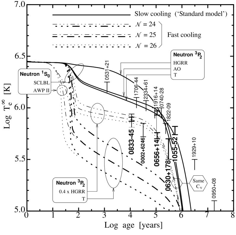
Figure 2.17: Typical behavior of slow (‘standard’) and fast cooling scenarios. 1.4 M_⊙neutron stars with the Friedman & Pandharipande (1981) equation of state. The cases with $\cal N$ = 24, 25, and 26 correspond approximately to the effect of a kaon condensate, pion condensate, and the direct URCA process (with hyperons or nucleons), respectively. The various curves, within each scenario, show the effect of various assumptions about pairing : all models use the proton ¹S₀ $T_{c}$ ‘T’, and the neutron ¹S₀ and ³P₂ $T_{c}$’s are as labeled. All models have non-magnetized iron envelopes. Neither Cooper pair breaking and formation neutrino emission nor heating are included. The main effect of pairing in the crust (neutron ¹S₀) is to shorten the length of the early plateau. Core pairing suppresses the neutrino emission, which results in a higher $T_{e}$ during the neutrino cooling era (age from $\sim$ 100 to $\sim$ 10⁵ yr), and the specific heat, which results in faster cooling during the photon cooling era (age above $\sim$ 10⁵ yr). The reduction of the specific heat during the neutrino cooling era does not show up as much as during the photon cooling era due to the small slope of the curves at this phase. All points are really upper limits (in several cases based on a non-detection of the pulsar) but for the radio pulsars 0833$-$45 (Vela), 0656+14, 0630+178 (Geminga), 1055$-$52, and the neutron star 0002+6246, there is good evidence that the observed X-rays are from surface thermal emission. Uncertainty on the temperature estimate is illustrated in the case of PSR 0656+14 where two values are reported [Page (1998].

In a recent work ?) have shown that a finite magnetic moment of neutrino would significantly modify the cooling history of a neutron star in the very early phases. This makes the crustal cooling compete with the core cooling within the typical time scale that conduction takes to transport thermal energy from the core to the surface.

It appears that the present data is compatible with both the slow and fast cooling processes (modified and direct URCA) as there is a lot of uncertainty in all the mechanisms involved in the thermal evolution of a neutron star. In figure [2.17] taken from ?) different theoretical scenarios could be seen and how these theories compare with the observational values of surface temperatures measured for various pulsars. There are other factors that may be responsible for a discrepancy between the theory of the thermal evolution of the neutron stars and the observed values for the surface temperatures. For example the temperature is usually estimated assuming the neutron star to behave like a perfect black-body, but the pressure of an atmosphere and the effects of a strong magnetic field may significantly modify this result [Pavlov et al. (1996, Shibanov & Yakovlev (1996].

2.3.2 thermal structure of an isolated neutron star

Temperature fluctuations in the interior of the neutron star are smoothed out very fast due to its large thermal conductivity and effectively the whole of the star behaves like an isothermal system, except at the layers close to the surface [Gudmundsson, Pethick, & Epstein (1982]. Though the temperature of the entire region beyond a density of $10^{10}~{}{\rm g}\,{\rm cm}^{-3}$ is practically the same, it drops by almost two orders of magnitude at the outermost layers of the star. The work of ?, ?) on the envelopes of non-magnetic neutron stars showed that the temperature of the isothermal interior, $T_{b}$, depends only on the surface temperature and the surface gravity of the star :

$$T_{b}=1.288\times 10^{8}K\left(\frac{(T_{s}/10^{6}K)^{4}}{g_{s}/10^{14}{\rm cm}{\rm s}^{-2}}\right)^{0.455}.$$

where $T_{s}$ is the surface temperature and $g_{s}$ is the surface gravity. These authors also present the variation of the temperature with density between the surface and the isothermal interior. To obtain temperature as a function of density in these outer regions of the crust we use the following fitting formula to their plots :

$$T(\rho)=(\frac{\rho}{\rho_{\rm boundary}})^{1/4}T_{b},\mbox{ $\rho\leq\rho_{\rm boundary}$}$$ (2.11)

where $\rho_{\rm boundary}$ is the density beyond which the temperature stays effectively constant.

2.3.3 accreting neutron star

The thermal history of an accreting neutron star is very different from that of an isolated one. The cooling of an isolated neutron star brings the surface temperature down to $\sim 10^{4.5}$ K in about $10^{7}$ yr with an attendant interior temperature of the nearly isothermal core of the order of $10^{7}$ K [van Riper (1991a]. Therefore when mass accretion starts this cold star is heated up due to the entropy inflow of the accreted matter. The temperature rise might be enough to start nuclear burning at the surface and one expects pycnonuclear shell burning of hydrogen and helium. Within a short time ($\sim 10^{5}$ yr) almost the entire crust is heated to a constant temperature of the order of $10^{7.5}-10^{8.5}$ K [Miralda-Escude, Paczynski, & Haensel (1990]. This is ignoring an initial short phase in which both the rate of accretion and the temperature of the crust show time evolution. The rate of accretion stabilizes in a few thousand years [Savonije (1978]. The temperature that the crust will finally attain in the steady phase has been computed by Fujimoto et ?), ?) and ?). However, these computations are restricted to limited range of mass accretion and also do not yield the same crustal temperature under similar conditions. The results obtained by ?) for the crustal temperatures for a given accretion rate in the range $10^{-15}$ M_⊙/yr$<\mbox{$\dot{M}$}<2\times 10^{-10}$ M_⊙/yr could be fitted to the following formula:

$$\log T=0.397\log\mbox{$\dot{M}$}+12.35.$$ (2.12)

But extrapolation of this fit to higher rates of accretion gives extremely high temperatures which would not be sustainable for any reasonable period due to rapid cooling by neutrinos at those temperatures. For the purpose of our calculations, we use equation [2.12] as long as the temperature of the crust is smaller than $10^{8.5}$ K. Beyond that we freeze the temperature at that upper limit. In figure [2.18] we have plotted the variation of the crustal temperature with accretion rate according to equation [2.12]. The thermal state of the core depends strongly on the neutrino emissivity whereas the crust remains largely indifferent to that. The core stays relatively cool if there is pion condensate inside which induces enhanced neutrino cooling, otherwise the core temperature may also be raised to a large extent by mass accretion.

Figure 2.18: Variation of the constant isothermal temperature of the crust of a neutron star with accretion rate.

The above discussion does not take into account the fact that the composition of the accreted layers could be very different from that of the original cold catalysed composition. In a recent work it has been shown that the presence of light elements in the accreted envelope enhances the emission processes in the photon cooling era and hence ultimately a faster cooling rate is achieved [Chabrier, Potekhin, & Yakovlev (1997, Potekhin, Chabrier, & Yakovlev (1997]. Such effects show drastic difference in the surface temperature (see [Page (1998] for a discussion) already within ten thousand years. If incorporated, this might change the evolution of the magnetic field considerably.

2.4 transport properties in the crust of neutron stars

The investigations of the transport properties of ultra-dense matter arise out of the interest in the evolution of the thermal state and the magnetic field in white dwarfs and neutron star crusts. See ?) and references therein for a good review on the transport properties of neutron star crust. It has already been mentioned in section [2.1] that the crust of a neutron star consists of a relativistic, Fermi-degenerate free electron gas plus a non-relativistic, non-degenerate liquid/crystal of ions. It is assumed that the material is completely pressure-ionized. The density at which this happens is given by the condition

$$\rho\geq 0.378AZ^{2}~{}{\rm g}\,{\rm cm}^{-3},$$ (2.13)

which turns out to be $\sim 10^{4}~{}{\rm g}\,{\rm cm}^{-3}$ for Fe⁵⁶ ions. Therefore, the lower boundary for which the transport properties have been worked out is this particular density. Though, recently, ?) have investigated the entire density range below this value.

The thermal and electrical conduction is basically carried out by the electrons. The electrical conductivity is given by following simple Drude formula [Ashcroft & Mermin (1979]

$$\sigma=\frac{n_{e}e^{2}\tau}{m_{\ast}},$$ (2.14)

where $n_{e}$ is the number density of electrons and $m_{\ast}$ is the effective mass of the electron in the crystal. $\tau$ is the time-scale of the collision of electrons with the ions (in liquid phase) or phonons/impurities (in case of a crystalline solid). It must be mentioned here that although the importance of quantum corrections have been realized in the present context, not much progress has been made in that direction

In the crust of a neutron star both density and temperature vary with radius. Whereas the uppermost layers close to the surface are likely to be in a liquid state, the inner crust is a crystalline solid. The condition for melting/crystallization of a classical one-component plasma is given by Lindeman criterion. According to this criterion [Slattery, Doolen, & Dewitt (1982],

$$\Gamma=\frac{\rm Coulomb\;Energy\;of\;the\;Crystal}{\rm Thermal\;Energy\;of\;the\;Lattice\;Ions},$$ (2.15)

equals 172 at the melting point. For a crystal composed of ionic species of charge $Z$ and lattice spacing $a$, the Coulomb Energy per ion is $\frac{(Ze)^{2}}{a}$ and the thermal energy of an ion is approximately $k_{B}T$ where $T$ is the temperature of the crystal. Therefore,

$$\Gamma=\frac{(Ze)^{2}}{ak_{B}T}.$$ (2.16)

The inter atomic spacing $a$, in terms of density is,

$$a=(\frac{4\pi}{3})^{-1/3}(\frac{\rho}{A})^{-1/3}m_{p}^{1/3},$$ (2.17)

$m$ and $A$ being the proton mass and the mass number of the ion, respectively. Then the melting temperature is

$$T_{m}=0.22692\times 10^{8}\frac{Z^{2}(\frac{\rho_{6}}{A})^{1/3}}{171}K,$$ (2.18)

where $\rho_{6}$ is the density in $10^{6}gm/cc$. In figure [2.19] the melting temperature has been plotted versus density in the crust of a 1.4 M_⊙ neutron star.

Figure 2.19: Variation of melting temperature with density in the crust on a neutron star.

Densities for which the actual temperature is above the melting temperature, the material is in a liquid state. The transport properties in such a state is determined by the electron-ion collisions and by electron-phonon collisions in the solid phase. The three factors important factors in calculating electron-phonon collision time-scale are - the dielectric screening of the phonon spectrum by the relativistic, Fermi-degenerate electrons, the Debye-Waller factor for the pure Coulomb, bcc crystal and the atomic form factor. The Debye-Waller factor changes the conductivity by a factor of two to four at the melting temperature. And when the electron de-Broglie wavelength becomes comparable to the nuclear size the third correction becomes rather important. Unlike the terrestrial situation, in the crust of a neutron star the Umklapp process dominates. For lower temperatures, the dominant process is that of the collision of electrons with the impurity atoms. These collisions are similar to the electron-ion collision in the liquid phase, except that here the effective charge is the difference between the charge of the impurity atom and the charge of the dominant species. The temperature or density of the cross-over from phonon dominated to impurity dominated process depends on the impurity strength $Q$, given by,

$$Q=\frac{1}{n}\sum_{i}{{n_{i}}(Z-Z_{i})^{2}}$$

where $n$ is the total ion density, $n_{i}$ is the density of impurity species $i$ with charge $Z_{i}$, and $Z$ is the ionic charge in the pure lattice [Yakovlev & Urpin (1980].

For our work, we have taken the expression for electrical conductivity of the liquid and due to impurity concentration in the solid from ?). For the pure crystalline phase we have used the results of ?). The conductivity in the liquid is given by,

$$\sigma_{\rm liquid}=8.53\times 10^{21}\frac{x^{3}}{Z\Lambda_{\rm Coulomb}(1+x^{2})},$$ (2.19)

where $x$ is defined by the relation

$$x=(Z/\rho_{6})^{1/3},$$ (2.20)

and $\Lambda_{\rm Coulomb}$ is the Coulomb logarithm. In the solid, the conductivity has contributions from both the phonon and the impurity processes. Therefore, the conductivity is given by,

$$\sigma_{\rm solid}=\frac{1}{\sigma_{\rm phonon}^{-1}+\sigma_{\rm impurity}^{-1}},$$ (2.21)

where

$$\sigma_{\rm impurity} = 8.53\times 10^{21}xZ/Q/s$$ (2.22)

$$\sigma_{\rm phonon} = 1.24\times 10^{20}\frac{x^{4}}{uT_{8}}\frac{(u^{2}+0.0174)^{1/2}}{(1+1.018x^{2})I_{\sigma}},$$ (2.23)

with,

$$u = \frac{2\pi}{9}(log\rho-3)$$

$$T_{8} = 10^{8}$$ temperature in units of K

$$\rho_{6} = 10^{6}~{}{\rm g}\,{\rm cm}^{-3}$$ density in units of

$$I_{\sigma} = \mbox{a function of density, $Z$, $A$ given by Itoh et al. 1984}.$$

In the following diagrams we have plotted the electrical conductivity in the crust of a neutron star, as a function of density and emphasizing the dependence on various parameters. In figure [2.20], the plot is for different values of the impurity concentration $Q$ for a given surface temperature. Notice that in this case we assume a temperature variation with density as is expected in a cool, isolated neutron star (section 2.3). In figure [2.21], on the other hand, we have plotted the conductivity for different values of the temperature which is constant over the whole of the crust. In figure [2.22], we have shown the change in conductivity with different values of $Q$, assuming the same constant crustal temperature in each case.

Figure 2.20: Variation of the electrical conductivity with density in the crust of a cool neutron star. The solid, dashed and dash-dotted curves correspond to $Q=0.0,0.01,0.1$. For all curves the surface temperature has been taken to be equal to $10^{4.5}$ K.

Figure 2.21: Variation of the electrical conductivity with density in the crust of a neutron star. The solid, dashed and dash-dotted curves correspond to the crustal temperatures of $10^{7.5},10^{8},10^{8.5}$ K. In all the curves $Q=0$.

Figure 2.22: Variation of the electrical conductivity with density in the crust of a neutron star. The solid, dashed and dash-dotted curves correspond to $Q=0.0,0.01,0.1$. For all curves $T=10^{8}$ K.

In figures [2.21] and [2.22] we have plotted the conductivity assuming the temperature to be constant over the entire crust. That is the case for a star with an accretion heated crust after the temperature has stabilized. For an isolated star with a very low surface temperature and a non-zero temperature gradient in the outermost layers (as described in section[2.3] above) the variation of conductivity with density looks somewhat different. In figure [2.20] we plot the conductivity profile for such a cool star. Note that the impurity strength $Q$ becomes important in this case.

It should be mentioned here that the above discussion does not refer to the fact that the transport properties in the crust of a neutron star must also take into account the presence of magnetic fields. As early as in 1980, Urpin & Yakovlev had looked into this problem. And recently, very refined results have been available in which conductivity calculations have been made with magnetic field [Potekhin, Chabrier, & Yakovlev (1997]. Also, all the above calculations have been made assuming a bcc lattice. Recently, ?) have also investigated the case of fcc lattice. But for our calculations we have not made use of these refined results.

Chapter 3 magnetic fields of neutron stars : a general introduction

3.1 overview

In the cosmic scheme of things the major players behind most of the interesting phenomena are rotation and magnetic field. A unique combination of very rapid rotation and a large magnetic field is what makes a neutron star act as a pulsar. The rotation period of a pulsar can be as small as 1.6 millisecond [Backer et al. (1982], and even the smallest field observed in pulsars could be about three orders of magnitude higher than the maximum field so far achieved in terrestrial laboratories. The typical values of magnetic field in pulsars range from $\sim 10^{8}$ Gauss to $10^{13.5}$ Gauss. It is the ultra-compact nature of a neutron star that allows the extremes in both the spin rate and the magnetic field strength. Because of the compactness it can support a fast rotation against the centrifugal forces and at close to nuclear densities even such high fields do not affect the state of the matter significantly because the energy associated with the magnetic field is insignificant compared to the other relevant energy scales [Shapiro & Teukolsky (1983].

It should also be noted that the neutron star material is something like the ultimate high-$T_{\rm c}$ super-conductor. Even though the temperature in the interior of a newly born neutron star could be about $10^{9}$K, it is still small compared to the superconducting transition temperature, believed to be a few times $10^{9}$K. Hence, the material inside a neutron star quickly settles into a superconducting state soon after its birth in a supernova explosion [Alpar (1991, Pines (1991]. We shall see later that this plays an important role in shaping the magnetic history of the star.

Unfortunately, there is as yet no satisfactory theory for either the generation of the neutron star magnetic field or its subsequent evolution [Bhattacharya (1995b]. There is a major uncertainty even about the possible location of the field in the interior of the star. This question is in fact related to the problem of the epoch and mechanism of field generation, as we shall see in the next section [Srinivasan (1995]. It is obvious that, under these circumstances, there can be no consensus regarding the theory of field evolution as any such scenario will have to ultimately depend on the nature of the underlying structure and location of the current loops that support the observable field.

Nevertheless, a compilation of current observational facts provides us with the nature of the questions that need to be looked into. They also give an indication of the range of possible answers. These observational facts strongly suggest that the field evolution is intricately related to the binary history of a neutron star. In the rest of this chapter we shall discuss the observational status and the current theoretical attempts to understand the generation and the subsequent evolution of the magnetic field in neutron stars. This provides the background for the problems addressed by us in chapters [4], [5], [6] and [7].

3.2 origin

There are two main possibilities regarding the generation of the magnetic field in neutron stars (for a review see [Bhattacharya & Srinivasan (1995], [Srinivasan (1995] and references therein). The field can either be a fossil remnant from the progenitor star, or be generated after the formation of the neutron star. Uncertainties surround both the scenarios and observations are yet to be able to distinguish between the two. This has led to a large variety of field evolution models that we shall discuss in section [3.3].

3.2.1 fossil field

Originally suggested by ?) and ?) long before the discovery of pulsars, the idea of the fossil field is considered to be the most promising. The magnetic field existing in the core of the progenitor star gets enhanced when the core collapses in a supernova, conserving the magnetic flux. Flux conservation demands an increase in the field strength by a factor $(R_{\rm progenitor}/R_{\rm NS})^{2}$ which is of the order of $10^{10}$. This can, depending on fields in the cores of the progenitor stars, produce fields as large as $10^{14}-10^{16}$ Gauss. The field observed on neutron stars is mainly the dipole component of the surface field. It is possible that the subsurface/interior field is much higher than this value.

In the core of a neutron star, the proton fraction is small (a maximum of 10% when presence of exotic states like Kaon condensates is considered [Pethick & Ravenhall (1992]. Nevertheless, the protons are believed to exist in a superconducting state. Calculations indicate that this is a type II superconductor with a lower critical field in excess of $10^{15}$ Gauss. Evidently, the observed field values fall far short of this critical field and one expects a complete flux expulsion in accordance with Meissner effect. But unlike in a laboratory situation the flux expulsion encounters a problem because the electrons coexisting with the protons do not form a condensate state. The time scale in which the flux can be expelled is therefore dictated by ohmic diffusion through the electron component. Even at extremely high temperatures at the time of the birth of the neutron star this ohmic diffusion time turns out to be larger than $10^{8}$ years. Hence, superconducting transition occurs with the field embedded in [Ginzburg & Kirzhnits (1964]. The magnetic field is carried in quantized flux tubes called Abrikosov fluxoids, each fluxoid carrying a quantum of magnetic flux, $\phi=\frac{hc}{2e}=2\times 10^{-7}$ G-cm². Therefore, some $10^{31}$ such fluxoids would be present in a neutron star with a typical field of $10^{12}$ Gauss.

One major problem with the concept of a fossil field is that strong surface fields are not observed in massive stars except in some dynamically peculiar ones. ?) suggest that the so-called fossil magnetic field may not be a relic of the main sequence phase of the star but can be generated in the core during the turbulent Carbon-burning phase. The strong field can therefore be hidden in the core, but given the short duration of evolution during and after the Carbon-burning phase, it is unclear whether this field can organize itself into large-scale poloidal components. A new input into the physics of the fossil field has come from the refined many-body calculations performed recently on the behaviour of the core superconductor. These new results hint that the core superconductor is likely to be of type I [Ainsworth, Wambach, & Pines (1989]. This would mean a completely different structure for the field and would require a redressal of some of the existing theories of field evolution involving flux expulsion associated with the spin-down of pulsars (discussed in subsection [3.3.1]).

3.2.2 post-formation field generation

Almost all of the existing field evolution models ultimately depend on ohmic dissipation of the currents in the crust of a neutron star, where the electrical conductivity, though very large by any terrestrial standard, is still finite (in contrast to the superconducting interior which can be thought to have an infinite conductivity). Therefore, any model that makes generation of currents in the crust possible is a very attractive proposition. We have mentioned earlier that the interior of a neutron star quickly settles into a superconducting state immediately after birth, as soon as its temperature falls below a few times $10^{9}$ K. This transition happens within a day or so after the formation of the star, and the observed field values are much smaller than the critical field of this superconductor. Hence, any field that is generated after the formation of the star has to be embedded in the region in which the protons are in a normal state. So post-formation generation mechanisms give rise to fields that are completely crustal and in particular confined to densities below neutron drip [Blandford, Applegate, & Hernquist (1983, Romani (1990, Urpin & Muslimov (1992a].

Following an idea originally proposed by ?), ?) worked out a possible mechanism for field generation. They suggested that magnetic field arises as a consequence of thermal effects occurring in the outer crust in the early phases of the thermal evolution of the star immediately after it is formed. The investigation is confined to the degenerate surface layers of non-rotating neutron stars, assuming that the plasma is in hydrostatic equilibrium. The density range considered is $\sim 10^{7}-10^{11}{\rm g}\,{\rm cm}^{-3}$, where the mechanism for field enhancement functions most effectively.

The field can grow either in the liquid phase and then be convected into the solid regions, or it could grow in the solid crust itself. In the solid, the heat flux is carried by the degenerate electrons giving rise to thermoelectric instabilities that in turn make the horizontal components of the magnetic field grow exponentially with time. The field grows with a time-scale of $\sim 10^{5}$ years. Such instability can also develop if the liquid phase that lies above the solid contains a horizontal magnetic field. The coexistence of a heat flux and a seed magnetic field, in excess of $10^{8}$ Gauss, in the liquid will cause the fluid to circulate which may lead to effective dynamo action. If that is the case then the field will grow rapidly, with a time scale of about a $10^{2}$ years, and supply the flux to the solid. Either of these two instabilities will soon saturate to produce a field strength of $\sim 10^{12}$ Gauss, where the instabilities become non-linear. Further growth will be prevented when either the magnetic stress exceeds the lattice yield stress or the temperature perturbations become non-linear, both of which happen at a subsurface field of $\sim 10^{14}$ Gauss. The corresponding surface field is $\sim 10^{12}$ Gauss.

The above mentioned mechanism is most effective for large temperature gradients. And the instabilities grow only if the ohmic diffusion time-scales are such that the increase in the field is not dissipated away at a faster rate than the growth. Unfortunately, for that to happen in the solid the conductivity should be at least a factor of three higher than the present estimates. Or if the surface layer is made of helium the instabilities can grow to large values. It must be noted here that the mechanism of field-growth mentioned here generates small loops only. The growth time-scales in the solid is too long which makes the field generation in the liquid layers the only viable option. The most effective way is to generate the flux in the liquid and then quickly anchor it in the solid crust either by advection of the flux or by freezing the liquid layer itself due to cooling of the star.

This work was extended for the case of rotating neutron stars by ?). They studied the thermo-magnetic instability in less deep and hence less dense liquid layers. In non-rotating neutron stars, the smearing of the instability due to hydrodynamic motions is an impediment to fast growth of field in the liquid. Fast rotations ($P\raisebox{-1.29167pt}{\mbox{$\stackrel{{\scriptstyle<}}{{{}_{\sim}}}\,$}}1$ s), however suppresses these hydrodynamic motions by Coriolis force. This mechanism is most effective when the electron temperature is $\raisebox{-1.29167pt}{\mbox{$\stackrel{{\scriptstyle>}}{{{}_{\sim}}}\,$}}3\times 10^{6}$ K and leads to the growth of an azimuthally symmetric toroidal magnetic field. Typical time-scale of field growth is of the order of a year and the typical horizontal wavelength is about 100 metres. The field is created at a depth of about 50 metres at density of the order of $10^{7}{\rm g}\,{\rm cm}^{-3}$.

The post-formation field generation mechanism is besieged by a number of problems, which were recognized by the early workers themselves. First and foremost is the fact that this mechanism is capable of generating only toroidal modes. And the scale-size of the field is confined to the melting depth of the crust which is of the order of hundred meters. In a series of papers, Geppert & Wiebicke (?, ?) and Wiebicke & Geppert (?, ?, ?, ?) have investigated the problem of field generation in the crust of neutron stars in detail. Their work reiterates the fact that the temperature gradient driven thermo-magnetic instability can only give rise to toroidal field, albeit strong. They have shown that it is possible to generate toroidal modes of very high polarities ($n\sim 1000$) in a short time ($\sim$ years) and that the magnitude of such field could also be quite large. But how such field could get restructured to a generate large-scale polar fields, the only kind that is actually observed in neutron stars, is still a point of much speculation.

As yet, there is no observational evidence for distinguishing one kind of field generation mechanism from the other. The only hope lies in the nature of the evolution of the field itself. Since the generation mechanism decides the question of underlying current structure, one expects that the predicted field evolution would be different for these two cases, and observations would be able to probe this difference. In chapter [8] we shall make some comments about the conclusions we have drawn regarding this problem from the nature of the field evolution and the evolutionary link between the population of normal pulsars and their millisecond counterparts.

3.3 evolution

The evolution of neutron star magnetic field has been of abiding interest both because it is a challenging problem in itself and also due to the fact that many other aspects of pulsar physics crucially depend on the nature of field evolution. Even though over the years a somewhat coherent picture has emerged, some of the key issues still remain unresolved. In particular, the generation of millisecond pulsars and their evolutionary link to the population of normal pulsars through a processing in binaries has become one of the major challenges that faces the researchers at present. There have been several excellent reviews detailing the current worries and the status of the theoretical endeavors [Bhattacharya (1995b, Bhattacharya (1995a, Bhattacharya & Srinivasan (1995, Ruderman (1995]. In this chapter, we shall recapitulate, in brief, the present situation, the observational indications and the theoretical models.

From observational facts and from the recent statistical analyses made on the pulsar population, the following conclusions can be drawn regarding the field evolution.

• Isolated pulsars with high magnetic fields ($\sim 10^{11}$ – $10^{13}$ G) do not undergo any significant field decay during their lifetimes [Bhattacharya et al. (1992, Wakatsuki et al. (1992, Lorimer (1994, Hartman et al. (1997].

• The fact that binary pulsars as well as millisecond and globular cluster pulsars which almost always have a history of being a member of a binary, possess much lower field strengths, suggests that significant field decay occurs only as a result of the interaction of a neutron star with its binary companion [Bailes (1996].

• The age determination of pulsars with white dwarf companions show that most of the millisecond pulsars are extremely long-lived. The old age ($\sim 10^{9}$ years) of the low-field pulsars implies that their field is stable over long time-scales. That is after the recycling process in the binaries is over, the field does not undergo any further decay [Bhattacharya & Srinivasan (1986, Kulkarni (1986, van den Heuvel, van Paradijs, & Taam (1986, Verbunt, Wijers, & Burm (1990].

• The evolutionary link between millisecond pulsars and low-mass X-ray binaries seem to be borne out both from binary evolution models and from the comparative study of the kinematics of these two populations. To spin a neutron star up to millisecond periods at least an amount $\sim 0.1\mbox{{\rm M}${}_{\odot}$}$ needs to be accreted. Such huge amount of mass transfer is possible only in low mass X-ray binaries, where the duration of mass transfer could be as long as $10^{9}$ years. And even though the present estimates for the birthrate of low mass X-ray binaries fall short of that of the millisecond pulsars [Kulkarni & Narayan (1988, Lorimer (1995], kinematic studies [Cordes et al. (1990, Wolszczan (1994, Nice & Taylor (1995, Nicastro & Johnston (1995, Bhattacharya (1996b, Ramachandran & Bhattacharya (1997, Cordes & Chernoff (1997], indicate that the two populations are most likely to be related as both have very similar kinematic properties.

3.3.1 models of field evolution

In order to understand the above facts, attempts have been made to relate the field decay to the star’s binary history. There are two classes of models which have been explored in this context one that relates the magnetic field evolution to the spin evolution of the star and the other attributing the field evolution to direct effects of mass accretion (see [Ruderman (1995] and [Bhattacharya (1995b] for detailed reviews). It should also be mentioned here that almost all the models are built upon two themes, namely, a large scale macroscopic restructuring of the fields in the interior of the star (for example, the spin-down and expulsion of flux from the superfluid core of the star) and a microscopic mechanism (like ohmic dissipation of the currents in the crust) acting to actually kill the underlying currents supporting the observable field. The different class of models usually assume different kind of initial field configuration. Models depending on spin-down assume a core-flux supported by proton superconductor flux tubes. Whereas, models invoking ohmic dissipation usually assume an initial crustal configuration. It should be noted here that a whole host of models exist that discuss field evolution of isolated neutron stars (for a list of such models see ?)). But we shall confine our discussion to accretion-induced models alone.

The former class of models involves the inter-pinning of the Abrikosov fluxoids (of the superconducting protons) and the Onsager-Feynman vortices (of the superfluid neutrons) in the core [Srinivasan et al. (1990, Ruderman (1991a]). This class also includes the models involving the plate tectonics of the neutron star crust [Ruderman (1991b, Ruderman (1991c]. ?) pointed out that neutron stars interacting with the companion’s wind would experience a major spin-down, causing the superconducting core to expel the magnetic flux, which would then undergo ohmic decay in the crust. This coupled evolution of spin and magnetic field has been modeled both for the cases of wide low mass X-ray binaries [Jahan Miri & Bhattacharya (1994] and high mass X-ray binaries [Jahan Miri (1996]. They have assumed ohmic decay of the expelled field in the crust with a constant decay constant of $10^{8}-10^{9}$ years. An investigation of the nature of the ohmic decay of such expelled field in an accretion heated crust has also been attempted [Bhattacharya & Datta (1996], and shows that the final field values could be quite consistent with those observed for millisecond pulsars. Ruderman (?, ?) on the other hand, suggests a coupling between the spin and the magnetic evolution of the star via crustal plate tectonics - torques acting on the star cause crustal plates, and the magnetic poles anchored in them, to migrate, resulting in major changes of the effective dipole moment.

The other class of models attribute the field decay to direct effects of accretion. The work done in this thesis comes under this category of models. Previous work by ?) and ?) have suggested that accreted matter might screen the pre-existing field. Computations by ?) indicate that hydrodynamic flows may bury the pre-existing field reducing the strength at the surface. We shall see in chapter[4] that strong Rayleigh-Taylor instabilities prevent such hydrodynamic flows to create horizontal components of the field at the expense of the dipolar component, and therefore such a screening mechanism does not provide for a viable scenario of field evolution in an accreting neutron star. The mechanism of ohmic decay, being unique to the crustal currents, is also used in models where spin-down is invoked for flux expulsion, for a subsequent dissipation of such flux in the crust [Jahan Miri & Bhattacharya (1994, Bhattacharya & Datta (1996].

The most important microscopic mechanism invoked for accretion-induced field decay is that of fast ohmic decay. In an accretion-heated crust the decay takes place principally as a result of rapid dissipation of currents due to the decrease in the electrical conductivity and hence a reduction in the ohmic dissipation time-scale [Geppert & Urpin (1994, Urpin & Geppert (1995, Urpin & Geppert (1996, Konar & Bhattacharya (1997]. The crustal field undergoes ohmic diffusion due to the finite electrical conductivity of the crustal lattice, but the time-scale of such decay is very long under ordinary conditions [Sang & Chanmugam (1987, Urpin & Muslimov (1992b]. The situation changes significantly when accretion is turned on. The heating of the crust reduces the electrical conductivity by several orders of magnitude, thereby reducing the ohmic decay time-scale.

There is also an additional effect that acts towards stabilizing the field. As the mass increases, a neutron star becomes more and more compact and the mass of the crust actually decreases by a small amount. So the newly accreted material forms the crust and the original crustal material gets continually assimilated into the superconducting core below. The original current carrying layers are thus pushed into deeper and more dense regions as accretion proceeds. The higher conductivity of the denser regions would progressively slow down the decay, till the current loops are completely inside the superconducting region where any further decay is prevented [Konar & Bhattacharya (1997].

3.3.2 the millisecond pulsar question

A summary of the current status of the important question of generation of millisecond pulsars has recently been presented by ?) in the proceedings of the IAU colloquium 160. The debate that followed the presentation (recorded in the same proceedings) gives a fair indication as to how bad the situation is. Here we shall just record the facts relevant to the field evolution, ignoring such questions that are associated with binary evolution and other factors.

In the fifteen years following the discovery of the first millisecond pulsar more than fifty pulsars have been discovered which belong to this particular category. In an attempt to understand the origin of millisecond pulsars, it was suggested that these are recycled pulsars, pulsars that have evolved to the characteristic magnetic field and spin-period by virtue of their binary history.

The major problem regarding the generation of millisecond pulsars in the binaries is the question of progenitors. What kind of binaries would give rise to millisecond pulsars? We have already mentioned that there is a problem of birthrate mismatch if one assumes that all the millisecond pulsars come from low mass X-ray binaries we normally observe. There is no satisfactory explanation for the origin of isolated millisecond pulsars either. Any model for field evolution has to be consistent with the nature of binary evolution that produced these objects. The field evolution scheme must also provide for a limiting minimum field strength—the so-called ‘flooring’ seen at $\sim 10^{8}$ G should arise out of the evolution itself. Except for a few of the models [Romani (1995, Jahan Miri & Bhattacharya (1994, Konar & Bhattacharya (1997] an explanation for this has not been attempted so far. And the models of field evolution must also match the spin-evolution of the neutron star in the binaries. Since there is no consensus on either the internal field structure or the evolution of the field, one important check on such models would be to look for a consistency of the field evolution models with that of the binary evolution scenario. In chapter[6] we attempt to look for such a consistency in general and from the point of view of millisecond pulsar generation in particular.

3.4 general introduction to accretion-induced field evolution

In the previous section we have seen that observational facts and statistical analyses of the existing data clearly relate the evolution of magnetic field of neutron stars with binary interaction. In the next chapter we shall address three different aspects of such binary-induced field evolution. We investigate the underlying physical mechanisms that take place in the interior of the star, changing the currents that are flowing to maintain the observable field. We would interest ourselves with a neutron star that is in active interaction with its binary companion. This companion could be a main sequence star affecting the neutron star through its wind. Alternatively, it could be a giant or a super giant, in which case heavy mass transfer may take place through Roche-lobe overflow [Bhattacharya & van den Heuvel (1991, King et al. (1995]. In either of these cases, there are some basic changes that the neutron star undergoes. These changes in various physical parameters are responsible for a change in the magnetic field. So, here is a brief resume of how the process of accretion affects a neutron star.

• The process of accretion mainly changes three parameters of the star, the total mass, the total angular momentum and the total energy. The change in energy comes about when the potential energy of the accreting particles get converted into random kinetic energy of the system and is then manifested as an increase in temperature.

• Models of field evolution have been proposed using the changes in each of these quantities, namely relating the change in the observable field $\delta B$ to $\delta M$ (change in mass), $\delta J$ (change in angular momentum) and $\delta T$ (change in temperature). In this connection it should be mentioned that earlier attempts to show a proportionality between $\delta B$ and $\delta M$ have recently been challenged [Wijers (1997].

• The change in angular momentum has been exploited in models which assume an initial field confined to the superconducting core of the star. In particular, a rapid slow-down ($\delta J\ll 0$) experienced by the neutron star during the ‘propeller phase’ causes the core field to be expelled to the crust, where it could undergo subsequent ohmic dissipation.

• Ultimately most of the accretion-related models depend on the ohmic dissipation of currents in the crust for a permanent decrease in the field. The rapidity of such dissipation depends on a decrease of the electrical conductivity, caused by an increase in the temperature ($\delta T\geq 0$).

• Another important factor influencing the field evolution is the hydrodynamic mass motion in the star. Near the surface the material flow is lateral, moving from polar (magnetic) to equatorial region. But interchange instabilities appear to prevent the screening of the field due to such hydrodynamic motions (chapter [4] of this thesis).

• Deep inside the star the material movement is a simple radial inflow, due to the compression of the star as a result of an increase in the total mass. The material movement is, evidently, a direct effect of the change in mass ($\delta M$), with the actual flow dynamics determined by the rate of such change, i.e., the rate of mass accretion, $\dot{M}$, on the star. This radially inward motion in the deeper layers helps to advect crustal currents to more dense layers, ultimately stabilizing the field in such cases.

From the above discussion, we see that processes of both macroscopic and microscopic nature are active in the interior of an accreting neutron star. The change in angular momentum induces a large scale flux movement whereas a change in total mass gives rise to large scale material movement. Both these cause macroscopic restructuring of the current pattern. On the other hand, a change in temperature induces the microscopic process of ohmic dissipation, by which the energy stored in the large scale field is transferred to the random kinetic energy of the particles. In the following sections, we shall see how these two mechanisms complement each other in the problems addressed by us.

Chapter 4 effect of diamagnetic screening

4.1 introduction

First proposed by ?), the idea of a possible screening of the magnetic field of a neutron star by accreting material onto it, has been a recurrent theme in the field-evolution scenario. This suggestion was substantiated by the work of ?) in which they indicated that the accreted matter, which is completely ionized plasma and hence diamagnetic in nature, might screen the pre-existing field reducing the strength of the surface field. Later ?) proposed a possible mechanism for such a screening. They suggested that the material accreting onto the poles of a magnetized neutron star will be confined by the strong magnetic stresses near the surface of the star. At low accretion rates the material sinks below the stellar surface until the hydrostatic pressure of the stellar material is as large as the magnetic pressure. The plasma then flows sideways giving rise to horizontal components of the magnetic field. The creation of this horizontal component comes at the expense of the vertical field and may result in a decrease in the observed field strength. This work, however, did not provide any quantitative details of the mechanism.

Later it was shown by ?) and ?) that the accretion column is actually like a small mountain on the polar cap rather than being subsurface. The accreting material is mostly ionized hydrogen and hydrogen has a smaller mean molecular weight per electron, $\mu_{e}$, than the iron crust of the star. Since most of the pressure in the accreted layer comes from the electrons, hydrogen tends to float over the underlying iron layer - if no material displacement perpendicular to the magnetic field is possible. A hydrogen mountain then forms at the surface of the neutron star. The height of this mountain depends on the density at which the transmutation of hydrogen (by electron capture on protons) takes place. When the material pressure in this accretion column becomes much larger than the magnetic pressure then the material starts flowing sideways giving rise to horizontal field components reducing the external dipolar field strength.

The first quantitative calculations of diamagnetic screening of neutron star magnetic field were performed by ?). It was shown in this work that hydrodynamic flows in the surface layers may bury the field to deeper layers effectively reducing the surface strength. In a later article [Romani (1995] in continuation to the earlier work, various time-scales, relevant for an effective screening of the surface field, were estimated. It was also shown here how the depth and density at which the field might get buried depend on the strength of the initial surface field.

In the present work, we investigate the effectiveness of diamagnetic screening as a possible mechanism for a permanent reduction in the surface field strength of the neutron stars. In particular, we shall try to answer the following questions :

1. Are diffusive time-scales, in the layers where the field is expected to be buried, long enough to allow screening to be an effective mechanism for long-term field reduction ?

2. Is it at all possible to bury the field or create horizontal components at the expense of the vertical one against Rayleigh-Taylor overturn instability ?

Recently, calculations of screening have been performed assuming the accreting material to be ferromagnetic [Zhang, Wu, & Yang (1994, Zhang (1998]. Such an assumption of extremely large magnetic permeability makes it possible to reduce the surface field by about four orders of magnitude. In our work though, we regard the accreting material to be completely ionized plasma (mainly hydrogen) and therefore to be diamagnetic in nature.

The layout of the chapter is in the following form. In section [4.2] we have discussed the nature of the material flow in an accreting neutron star. In section [4.3] we discuss the actual mechanism of the diamagnetic screening and the various relevant time-scales. And finally in section [4.4] we present our conclusions.

4.2 accretion and material flow

For a neutron star with a strong magnetic field, the flow of the accreting material outside the star is completely determined by the field. The material flows in along open field lines and hits the surface within the polar cap region. The area of this polar cap region is determined by the rate of accretion and the strength of the magnetic field [Shapiro & Teukolsky (1983]. In all our subsequent discussions we shall assume a situation where the magnetic axis and the rotation axis are aligned. Even though that is hardly ever the case in reality, this assumption does not affect the general conclusions much.

The polar cap area, region constrained by open field lines on the surface of the star, is given by,

$$A_{P}=2\pi R_{s}^{2}[1-\cos\theta],$$ (4.1)

where, $R_{s}$ is the radius of the star and $\theta$ is the angle the last open field line makes with magnetic axis. This limiting field line is the one which goes through the Alfvén radius, $R_{A}$, in the equatorial plane. Therefore, using the equation for the dipole field lines one finds $\sin\theta=\sqrt{\frac{R_{s}}{R_{A}}}$, so that the polar cap area is given by,

$$A_{P}=2\pi R_{s}^{2}\left[1-\sqrt{1-\frac{R_{s}}{R_{A}}}\right].$$ (4.2)

In the limit $R_{A}>>R_{s}$ (which is a reasonable approximation for the range of field strength and accretion rate we consider), the above expression reduces to the following simple form :

$$A_{P}=\pi\frac{R_{s}^{3}}{R_{A}}.$$ (4.3)

The Alfvén radius of an accreting system is determined by the condition that at this radius the ram pressure of the in-falling material equals the pressure of the magnetic field. The ram pressure at the Alfvén radius is :

$$P_{\rm ram}=\frac{1}{2}\rho(R_{A})V^{2}(R_{A}),$$ (4.4)

where $\rho(R_{A})$ is the density and $V(R_{A})$ is the velocity of the accreting material at Alfvén radius. In an accretion disc material rotates with Keplerian velocity at every radius. Therefore, the velocity of the material at Alfvén radius is given by,

$$V(R_{A})=(\frac{GM}{R_{A}})^{1/2}.$$ (4.5)

The density of the accreting material at Alfvén radius is :

$$\rho(R_{A})=\frac{\mbox{$\dot{M}$}}{4\pi V(R_{A})R_{A}^{2}},$$ (4.6)

where, the dependence on the rate of mass accretion is quite obvious. As the field is dipolar in nature, the field strength at the Alfvén radius is,

$$B(R_{A})=(\frac{R_{s}}{R_{A}})^{3}B_{s},$$ (4.7)

where, $B_{s}$ stands for the strength of the field at the surface of the neutron star. Equating the ram pressure and the magnetic pressure, one obtains the following expressions for the Alfvén radius and the polar cap area respectively,

$$R_{A} = (2GM)^{-1/7}R_{s}^{12/7}B_{s}^{4/7}{\mbox{$\dot{M}$}}^{-2/7}$$ (4.8)

$$A_{P} = \pi(2G)^{1/7}M^{1/7}R_{s}^{9/7}B_{s}^{-4/7}{\mbox{$\dot{M}$}}^{2/7}.$$ (4.9)

The density profile within the accretion column is described by an ‘atmosphere’ solution [Bildsten & Cutler (1995]. The pressure in the column, due to the relativistic degenerate electrons and the ions, is given by

$$P=\frac{1}{4}n_{e}m_{e}c^{2}x+n_{I}k_{B}T,$$ (4.10)

where $n_{e}(n_{I})$ is the number density of electrons (ions) and $m_{e}$ is the electron mass. $x$ is the relativity parameter defined as

$$x = \frac{p_{F}}{m_{e}c}$$ (4.11)

$$= 1.008(\frac{Z\rho_{6}}{A})^{1/3},$$

where $p_{F}$ is the Fermi momentum of the electrons, $(Z,A)$ correspond to the atomic number and mass number of the dominant ion species and $\rho_{6}$ is density in units of $10^{6}{\rm g}\,{\rm cm}^{-3}$. The scale height of the accretion column is given by $H=\frac{P}{\rho g}$, where $\rho$ and $P$ are the density and pressure respectively at the base of the accretion column and $g$ is the acceleration due to gravity at the surface of the state. Using the above equation of state the scale height, for a $1.4~{}\mbox{{\rm M}${}_{\odot}$}$ star, is approximately found to be :

$$H\sim 324\;\rho_{6}^{1/3}{\rm cm}.$$ (4.12)

As long as the pressure in the accretion column is much smaller than the magnetic pressure there can not be any material movement across the field lines so the accreted material remains confined to the polar cap. This kind of polar cap accretion causes transverse pressure gradients that are balanced by the curvature of the magnetic field. An order of magnitude estimate by Hameury et al. ?) shows that in order to create a significant distortion of the field lines due to the overpressure of the accretion column the condition

$$\frac{P_{\rm accretion}}{P_{\rm magnetic}}\raisebox{-1.29167pt}{\mbox{$\stackrel{{\scriptstyle>}}{{{}_{\sim}}}\,$}}\frac{R_{P}}{H}$$ (4.13)

should be satisfied. Here, $P_{\rm accretion}$ and $P_{\rm magnetic}$ stand for pressure due to the material in the accretion column and due to the magnetic field respectively. $R_{P}$ is the radius of the polar cap and $H$ is the density scale height of the accretion column. For a given value of the crustal field and a given rate of accretion, the density at which the material starts flowing sideways, obtained from the condition given by equation [4.13], is :

$$\rho_{\rm flow}=2.0961\times 10^{8}B_{13}^{36/35}\mbox{$\dot{M}$}_{-9}^{3/35},$$ (4.14)

where $B_{13}$ is the field strength in units of $10^{13}$ Gauss and $\mbox{$\dot{M}$}_{-9}$ is the accretion rate in units of $10^{-9}$ M_⊙ yr^-1. This condition is, of course, only valid in absence of any interchange instabilities about which we shall discuss later. In figure [4.1] we plot the variation of the flow density with the field strength for various values of the accretion rate.

Figure 4.1: Variation of the flow density with the surface fields strength. The different curves (from top to bottom) correspond to $\mbox{$\dot{M}$}=10^{-8},10^{-8.5},10^{-9},10^{-9.5},10^{-10}$ M_⊙ yr^-1respectively.

4.3 physics of diamagnetic screening

We shall, as has been mentioned above, work under the assumption of a flux-frozen situation. This basically amounts to assuming an effectively infinite conductivity. Admittedly, even though large, the actual value of conductivity is finite. But the large values of conductivity in crust provide for extremely long diffusive time-scales. In this case, the assumption of ‘flux-freezing’ is a valid one since the flow time-scales are much smaller compared to this diffusive time-scale (to be discussed in the next section).

Therefore a reduction in the surface field is obtained due to the combined effect of i) flux freezing and ii) hydrodynamic flow of the material. Due to flux-freezing the total flux contained within an amount of material remains constant. And when this material flows and spreads out covering a larger area, the field gets adjusted to keep the flux conserved. Say, the total flux contained within the polar cap at time $t=0$ is $B\times A_{P}$. Conservation of flux then implies that we have,

$$\frac{dB}{dt}\times A_{P}+B\times\frac{dA_{P}}{dt}=0.$$ (4.15)

Therefore the change in the field strength is related to the change in the area of the original polar cap surface due to material flow during accretion. Assuming that the flow of material is such that at each instant the amount accreted equals the amount flowing out from under the accretion column one obtains the following relation between the change in the polar cap area and the rate of mass accretion $\dot{M}$ given by,

$$\mbox{$\dot{M}$}dt=\rho_{\rm flow}h_{\rm flow}dA_{P}$$ (4.16)

where, $dA_{P}$ is the change in the polar cap area in time $dt$. $\rho_{\rm flow}$ is the density where the flow takes place and $h_{\rm flow}$ is the effective height of the accretion column, which hereafter we take roughly to be equal to the density scale height $H$. Integrating equation [4.16] above the time variation of the polar cap area is obtained in the following form -

$$A_{P}(t)=A_{P}(t=0)+\frac{\mbox{$\dot{M}$}t}{\rho_{\rm flow}H},$$ (4.17)

where, $A_{P}(t=0)$ is the original area of the polar cap. Then equation [4.15] implies the following time dependence of the surface field :

$$B(t)=\frac{B_{0}}{[1+\frac{t}{\tau_{\rm screen}}]},$$ (4.18)

where we have defined the screening time-scale by the relation

$$\tau_{\rm screen}=\frac{\rho_{\rm flow}HA_{P}}{\mbox{$\dot{M}$}}.$$ (4.19)

This is the time in which the original field reduces to half of its original value. It should be noted here that ?) obtained an expression for the decay of magnetic field due to accretion very similar to equation [4.15] from purely phenomenological considerations. Here we have arrived at the above relation from a more physical point of view.

To find the effectiveness of the screening we need to compare this time-scale to the diffusive time-scale over which the field may re-emerge by ohmic diffusion through the overlaying layers. The diffusive time-scale is defined by,

$$\tau_{\rm diff}=\frac{4\pi\sigma(\rho_{\rm flow},T({\mbox{$\dot{M}$}}))H^{2}}{c^{2}},$$ (4.20)

where, $\sigma$ is the electrical conductivity which is a function of the density and the crustal temperature. We shall show later that if one ignores interchange instabilities, then the flow time scale is much smaller than diffusion time scale, and therefore field would remain frozen and be dragged. Reconnection will then occur on the equatorial plane and that will bury the field. Before this field can diffuse out more matter will come and spread on top of it, and drive the field deeper. So the eventual re-emergence time scale is set not by the initial depth at which it was buried but the final depth to which it is driven by continuous accretion. This can be very deep and the field can even reach the core and therefore never get out again. But for the moment, we take the burial depth to be equal to the scale height of the density. For the screening time-scale this, of course, is the actual length-scale. For the diffusive case we find the time-scale at the depth where the field gets buried to begin with. We have not considered the case of deep burial mentioned above, since from the subsequent discussion that will prove to be unnecessary.

The point to be noted here is that for the screening mechanism described above the important factor is the anisotropic material flow through the polar cap. The area of polar cap increases with increasing rate of accretion. Hence, for low rates of accretion, the flow is maximally anisotropic. For high values of accretion rate, the polar cap could cover a large fraction of the stellar surface area. The effect of anisotropic material flow would not be very severe in that case. Also as mentioned earlier, the temperatures are higher for higher values $\dot{M}$, a lower value of conductivity and therefore a smaller diffusive time. Hence, situations with low values of $\dot{M}$ has better chance of screening the field.

In all of the above discussion, the implicit assumption has been that it is possible to create a horizontal component of the magnetic field, at the expense of the vertical component, as a result of material flow in a ‘flux-frozen’ condition. But this mechanism is not viable against the Rayleigh-Taylor instability. This instability arises due to magnetic buoyancy. As the accreting material slowly builds up in a column, the field lines tend to spread out due to the diamagnetic property of the material. At the base of the accretion column, the field lines are firmly anchored to the solid crust. Therefore material flow at the base of the accretion column stretches the field lines out horizontally. This creates horizontal components of the field giving rise to a screening of the external dipole. We have seen earlier that the pressure of the accretion column is much larger than the pressure of the magnetic field in this region. Under such a condition the field lines re-organize themselves into flux tubes as that is the minimum energy configuration. These flux tubes move upward due to magnetic buoyancy and thereby destroy the horizontal component of the field (see [Spruit (1983] and references therein).

In a tube in pressure equilibrium with its surroundings the pressure is

$$P_{\rm in}+P_{\rm magnetic}=P_{\rm out}.$$ (4.21)

However at the base of the accretion column $\beta\equiv\frac{P_{\rm gas}}{P_{\rm magnetic}}\sim\frac{R_{P}}{H}$ and the above relation simplifies to

$$P_{\rm in}=(1-1/\beta)P_{\rm out}.$$ (4.22)

Therefore, the gas pressure within a flux tube is smaller than the gas pressure outside. Then from equation [4.10] we find the following relation between internal and external densities :

$$\rho_{\rm in} = (1-1/\beta)^{3/4}\rho_{\rm out}$$

$${\rm or}$$

$$\frac{\delta\rho}{\rho_{\rm in}} = \frac{3}{4\beta},$$ (4.24)

where $\delta\rho$ is the density deficit within the flux tubes. This density deficit makes the flux tube move upward under the force of buoyancy. The upward velocity $V_{F}$ of the flux tubes is given by the equality of the buoyancy force with the aerodynamic drag force per unit area of the flux tube :

$$\frac{1}{2}\rho_{\rm in}V_{F}^{2}=g\,r\,\delta\rho,$$ (4.25)

where $r$ is the characteristic radius of the flux tube and $g$ is the acceleration due to gravity. Therefore, the velocity is :

$$V_{F}=\sqrt{\frac{3gr}{2\beta}}$$ (4.26)

and the time-scale required for a flux-tube to traverse the density scale-height is :

$$\tau_{\rm RT}=\frac{H}{V_{F}}.$$ (4.27)

It should be noted that the characteristic scale length of the flux tubes is again that of the density scale-height, and therefore,

$$\tau_{\rm RT}=\sqrt{\frac{2\beta H}{3g}}.$$ (4.28)

The time-scale for the reconnection of the field lines, on the other hand, is typically given by

$$\tau_{\rm recon} = \frac{l_{\rm instability}}{V_{A}},\mbox{ if $V_{A}<V_{S}$}$$ (4.29)

$$= \frac{l_{\rm instability}}{V_{S}},\mbox{ if $V_{S}<V_{A}$};$$

where, $V_{A},V_{S}$ are the Alfvén and the sound speed, respectively. $l_{\rm instability}$ is the length-scale of the instability which is again of the order of the density scale height in the accretion column. Within the accretion column the sound speed is always much greater than the Alfvén velocity and therefore only the top expressions of the above equations are relevant here. At the flow density, the Alfvén velocity is

$$V_{A}=\frac{B}{\sqrt{4\pi\rho_{\rm flow}}}.$$ (4.30)

Therefore, the expressions for the reconnection time-scale is given by

$$\tau_{\rm recon} = \frac{H\sqrt{4\pi\rho_{\rm flow}}}{B},$$ (4.31)

For the screening to be effective, the total time taken to create a loop of field lines by turn-over instability and to destroy the loop by reconnection has to be much larger than the screening time-scale defined above. So we define an instability time-scale as

$$\tau_{\rm instability}=\tau_{\rm RT}+\tau_{\rm recon}$$ (4.33)

which should be compared with $\tau_{\rm screen}$. It must be noted here that we use the ‘pressure scale-height’ and ‘density scale-height’ interchangeably in the above discussion since for barotropic (atmospheric) equation of state (as is the case here) a pressure gradient implies the same density gradient.

Figure 4.2: Variation of the time-scales with surface fields strength. The (a), (b), and (c) groups of curves correspond to diffusive, screening and instability time-scales respectively. The curves (in each group) correspond to $\mbox{$\dot{M}$}=10^{-10},10^{-9.5},10^{-9},10^{-8.5}$ M_⊙ yr^-1respectively, the upper curves being of lower values of accretion.

Therefore the three relevant time-scales of the problem are :

• screening time-scale - given by equation [4.19];

• diffusive time-scale - given by equation [4.20]; and

• instability time-scale - given by equation [4.33].

In figure[4.2] we plot all the time-scales as functions of surface field strength and the accretion rate.

4.4 discussion and conclusions

Looking at the figures plotted above, obtained for a range of values for the accretion rate and the surface field strength, we find that,

1. The density of flow increases with an increase in the field strength. The larger the field, the deeper and denser it gets buried (see figure [4.1]). The flow density also has a mild positive dependence on the rate of mass accretion. But even for very large values of the surface field strength the flow does not occur at densities beyond $\sim 10^{9}~{}{\rm g}\,{\rm cm}^{-3}$. That means the flow always takes place within the liquid layer. And the earlier contentions of a burial within the solid layer does not really happen.

2. As the screening time-scales are always much smaller than the diffusive time-scales a condition of flux-freezing prevails and material movement indeed should proceed dragging the field lines along.

3. But, since the instability time-scale (sum of the overturn and the re-connection time-scales) is much too smaller than the other two time-scales of the problem, any stretching of field line is quickly restored (over the instability time-scale) and the material effectively flows past the field lines without causing any change.

We find that the time-scale of overturn and reconnection is so much smaller than any other time-scale of the problem that it is not at all possible to create horizontal field components at the cost of vertical ones and effect a screening. Therefore, it is not possible to screen the magnetic field of a neutron star by the accreting material in order to reduce the magnitude of the external dipole observed.

Chapter 5 evolution of crustal magnetic field in an accreting neutron star

5.1 introduction

It has been discussed in chapter [3] that observations suggest a connection between the low magnetic field of binary and millisecond pulsars and their being processed in binary systems, indicating accretion-induced field decay in such systems. A possible mechanism for such decay is understood to be the rapid ohmic dissipation of the currents in the accretion heated crust (see section [3.3] for details). In this work we explore models that primarily depend on this microscopic process of ohmic decay for a permanent reduction in the observed field strength, and also on the large scale material movement for the final stabilization of the field. Here we shall investigate a model based on the assumption that the current loops responsible for the magnetic field are initially confined entirely within the crust. This situation is likely to be the result of a generation of the field due to thermo-magnetic instabilities after the birth of the star (see section [3.2] for details). If the initial field resides mainly in the superconducting core then our scenario would apply only after most of this flux has been expelled into the crust, a situation which will be treated in chapter [7].

The crustal field undergoes ohmic diffusion due to the finite electrical conductivity of the crustal lattice, but the time-scale of such decay is very long under ordinary conditions [Sang & Chanmugam (1987, Urpin & Muslimov (1992b]. The situation changes significantly when accretion is turned on. The heating of the crust reduces the electrical conductivity by several orders of magnitude, thereby reducing the ohmic decay time-scale. As the mass increases, a neutron star becomes more and more compact and the mass of the crust actually decreases by a small amount (see section [2.2]). So the newly accreted material forms the crust and the original crustal material gets continually assimilated into the superconducting core beneath. The original current carrying layers are thus pushed into deeper and more dense regions as accretion proceeds. This compression results in a decrease of the effective length scale of the current loops which makes a fast dissipation possible [Konar, Bhattacharya, & Urpin (1995]. But the higher conductivity of the denser regions would progressively slow down the decay winning over the effect of a decrease in the length scale, till the current loops are completely inside the superconducting region where any further decay is prevented.

The organization of the chapter is as follows. In section [5.2] we discuss the physics of the field reduction in an accreting neutron star, computational details are discussed in section [5.3]. Finally in section [5.4] we present our results and draw the conclusions in section [5.5].

5.2 physics of the mechanism

The evolution of the crustal field as a result of ohmic diffusion and material motion has been discussed by a number of authors [Wendell, van Horn, & Sargent (1987, Sang & Chanmugam (1987, Geppert & Urpin (1994] and essentially concerns the solution of the following equation [Jackson (1975]

$$\frac{\partial\vec{B}}{\partial t}=\vec{\nabla}\times(\vec{V}\times\vec{B})-\frac{c^{2}}{4\pi}\vec{\nabla}\times(\frac{1}{\sigma}\times\vec{\nabla}\times\vec{B})$$ (5.1)

where $\vec{V}$ is the velocity of material movement and $\sigma$ is the electrical conductivity of the medium. As in previous studies we solve this equation by introducing the vector potential $\vec{A}$, such that

$$\vec{B}=\nabla\times\vec{A}$$ (5.2)

where, ${\vec{A}}=(0,0,A_{\phi})$. This choice of the vector potential ensures a poloidal geometry for $\vec{B}$. In particular, we choose

$$A_{\phi}=\frac{g(r,t)\sin\theta}{r},\;\mbox{$g(r,t)$ is the Stokes' function},$$ (5.3)

$(r,\theta,\phi)$ being the spherical polar co-ordinates. Here we work in the lowest order of multipole, obtaining the following dipolar form of the magnetic field :

$$\vec{B}(r,\theta) = \vec{\nabla}\times(\frac{g(r,t)\sin\theta}{r}\;\hat{\phi})$$ (5.4)

$$= \frac{2\cos\theta g(r,t)}{r^{2}}{\hat{r}}-\frac{\sin\theta}{r}\frac{\partial g(r,t)}{\partial r}{\hat{\theta}}.$$

The magnitude of the field is given by,

$$B(r,\theta)={\left[\frac{4\cos^{2}\theta g^{2}(r,t)}{r^{4}}+\frac{\sin^{2}\theta}{r^{2}}(\frac{\partial g(r,t)}{\partial r})^{2}\right]}^{1/2}$$ (5.5)

Therefore, at the pole ($\theta=0$, $r=R$) the magnitude is

$$B(R,0)=\frac{2g(R,t)}{R^{2}},$$ (5.6)

which is simply proportional to the value of the Stokes’ function there. We shall use this fact to obtain the evolution of the surface field with time.

The underlying current distribution corresponding to the above field is obtained by using Maxwell’s equation :

$$\vec{J} = \frac{c}{4\pi}\nabla\times\vec{B}$$ (5.7)

$$= -\frac{c}{4\pi}\;\frac{\sin\theta}{r}\left[\frac{\partial^{2}g(r,t)}{\partial r^{2}}-\frac{2\,g(r,t)}{r^{2}}\right]{\hat{\phi}}.$$

5.2.1 ohmic diffusion

In order to understand the ohmic dissipation of the field strength, let us consider equation [5.1] without the first term on the right hand side. The first term corresponds to the convective transport, which we shall discuss later. Without this term equation [5.1] takes the following form,

$$\frac{\partial\vec{B}}{\partial t}=-\frac{c^{2}}{4\pi}\vec{\nabla}\times(\frac{1}{\sigma}\times\vec{\nabla}\times\vec{B}).$$ (5.8)

For the moment, let us consider the conductivity to be a constant, without any dependence on space. Then, the above equation takes the form of a pure diffusion equation (by virtue of the divergence-free condition for the magnetic fields), given by

$$\frac{\partial\vec{B}}{\partial t}=\frac{c^{2}}{4\pi\sigma}\nabla^{2}\vec{B}.$$ (5.9)

The diffusion constant for the above equation is $\frac{c^{2}}{4\pi\sigma}$. One can define a time-scale characteristic of the diffusion process :

$$\tau_{\rm diff}=\frac{4\pi\sigma L^{2}}{c^{2}},$$ (5.10)

where $L$ is the length-scale associated with the underlying current distribution supporting the field.

It is clear from equation [5.10] that the rate of ohmic diffusion is determined mainly by the electrical conductivity of the crust which is a steeply increasing function of density (see figures in section [2.4]). As density in the crust spans eight orders of magnitude with a very large radial gradient the conductivity changes sharply as a function of depth from the neutron star surface. Thus the deeper the location of the current distribution, the slower is the decay. We have discussed, in detail, the effects of temperature and that of impurity concentration on the conductivity in section [2.4], also about the change in the thermal behaviour in presence of accretion in a neutron star in section [2.3]. The increase in temperature of an accretion-heated crust lowers the conductivity and therefore the time-scale for the diffusion decreases. In other words, the transfer of the energy of the systematic motion of the charge carriers (the electrons) within the current loops into the random kinetic energy of the electrons proceed at a faster rate at a higher temperature. For the models we are considering now, it has been assumed in the literature that the impurity strength $Q$ lies in the range 0.01 - 0.1. The effect of impurities is most important at lower temperatures and higher densities (see figures [2.21] and [2.22]). Therefore the field evolution does not show any significant dependence on impurity strength for this range of $Q$ in an accretion-heated crust. We therefore restrict our computations to the $Q=0.0$ case. However, the impurity strength will still play an important role in field decay during the pre-accretion phase when the crustal temperatures can be quite low.

5.2.2 accretion and material transport

In a neutron star, for a given equation of state, the mass of the crust is uniquely determined by the total mass of the star (see section [2.2]). And this crustal mass remains effectively constant for the accreted masses of the order of 0.1 M_⊙  with a slight decrease as the total mass increases (see figures [2.14], [2.15] and [2.16]). For example, for the equation of state that we have used (see section [2.1] for details) the accretion of 0.1 M_⊙ on the star causes a change in the crustal mass of only 0.004 M_⊙. As a result, accretion causes continuous assimilation of material from the bottom of the crust into the core. At the same time the upper layers of the original crust are pushed to deeper and denser regions, leading to extreme squeeze of this material. This also causes the current distribution embedded in this material to be sharpened, reducing the effective length scale of the system.

The change in the crustal mass and the crustal density profile is negligible for the amount of mass accretion we consider. We therefore take the mass flux to be the same throughout the crust, equal to its value at the surface. Assuming the mass flow to be spherically symmetric in the crustal layers of interest, one the obtains the following condition for the equality of mass flux at all densities within the crust,

$$\mbox{$\dot{M}$}dt = 4\pi r^{2}\rho(r)dr,$$

$$\Rightarrow V(r) = \frac{\mbox{$\dot{M}$}}{4\pi r^{2}\rho(r)},$$ (5.11)

where $\dot{M}$ is the rate of mass accretion and $\rho(r)$ is the density as a function of radius $r$. The above equation defines $V(r)$ - the velocity of radial material flow at a given radius in the crust. It should be noted here that the material flow is radially inwards, hence writing the flow velocity in its full vectorial form we have,

$$\vec{V}(r)=-\frac{\mbox{$\dot{M}$}}{4\pi r^{2}\rho(r)}{\hat{r}}.$$ (5.12)

The result of accretion on the magnetic field evolution therefore manifests itself as a combination of three effects: transport of the current distribution to regions of higher density and hence higher conductivity, reduction of conductivity due to heating and change in the effective length scale of the current distribution (see [Bhattacharya (1995b] for a detailed discussion). We find that the overall effect turns out to be a rapid initial decay followed by a leveling off when an amount of mass equivalent to about 10% of the original crust has been accreted. By this time the current loops reach the regions of very high density and consequently of extremely large conductivity where the diffusion time-scales are much too long. As further accretion proceeds the original crust is assimilated into the superconducting interior freezing the currents there. Following ?) we assume that the newly formed superconducting material retains the magnetic flux through it in the form of Abrikosov fluxoids rather than expelling it through the Meissner effect.

5.2.3 the field evolution equation

We use the form of $B(r,\theta,\phi)$ given by equation [5.4] and the form of $\vec{V}$ given by equation [5.12] to cast equation [5.1] in terms of the Stokes’ function.

1. The left hand side –

   $$\frac{\partial\vec{B}}{\partial t} = \frac{\partial\nabla\times\vec{A}}{\partial t}$$ (5.13)

   $$= \nabla\times\frac{\partial}{\partial t}\;\left[\frac{g(r,\theta)\;\sin\theta}{r}\right]\;{\hat{\phi}}.$$

2. The first term in the right hand side –

   $$\nabla\times(\vec{V}\times\vec{B}) = \nabla\times\left[\left(-V(r)\;{\hat{r}}\right)\times\left(\frac{2\cos\theta\;g(r,t)}{r^{2}}{\hat{r}}-\frac{\sin\theta}{r}\;\frac{\partial g(r,t)}{\partial r}\;{\hat{\theta}}\right)\right]$$ (5.14)

   $$= \nabla\times\left[\frac{\sin\theta\;V(r)}{r}\;\frac{\partial g(r,\theta)}{\partial r}\right]\;{\hat{\phi}}.$$

3. The second term in the right hand side –

   $$\nabla\times\left[\frac{1}{\sigma}\nabla\times\vec{B}\right] = \nabla\times\left[\frac{1}{\sigma}\nabla\times\left(\frac{2\cos\theta\;g(r,t)}{r^{2}}\;{\hat{r}}-\frac{\sin\theta}{r}\;\frac{\partial g(r,t)}{\partial r}\;{\hat{\theta}}\right)\right]$$ (5.15)

   $$= \nabla\times\left[-\frac{1}{\sigma}\;\frac{\sin\theta}{r}\;\left(\frac{\partial^{2}g(r,t)}{\partial r^{2}}-\frac{2g(r,t)}{r^{2}}\right)\;{\hat{\phi}}\right].$$

Incorporation of the expressions [5.13], [5.14] and [5.15] in the equation[5.1] then leads to

$$\frac{\partial g(r,t)}{\partial t}=V(r)\frac{\partial g(r,t)}{\partial r}+\frac{c^{2}}{4\pi\sigma}\left(\frac{\partial^{2}g(r,t)}{\partial r^{2}}-\frac{2g(r,t)}{r^{2}}\right).$$ (5.16)

The results of this chapter will be based on numerical solutions of the equation [5.16].

5.3 computations

The aim of our computations is to solve equation [5.16] to obtain $g(r,t)$ using the following boundary conditions valid for all times (see, e.g., Geppert & Urpin 1994):

$$\frac{\partial g(r,t)}{\partial r}|_{r=R}+\frac{g(R,t)}{R}=0,$$ (5.17)

$$g(r_{\rm co},t)=0$$ (5.18)

where $R$ is radius of the star and $r_{\rm co}$ is that radius to which the original boundary between the core and the crust is pushed to, due to accretion, at any point of time. The first condition matches the interior field to an external dipole configuration. The second condition indicates that as accretion proceeds along with the crustal material the frozen-in flux moves inside the core, but the field can not diffuse through the original crust-core boundary. To simulate an effectively infinite conductivity in the region between the bottom of the crust and the original boundary between the crust and the core, we set $\sigma\sim 10^{50}{\rm s^{-1}}$ in this region. As mentioned before, we take into account the combined effects of accretion driven material motion and ohmic diffusion. We construct the density profile of a neutron star as described in section [2.2] for an assumed mass of 1.4 M_⊙. This star has a total crustal mass of 0.044 M_⊙ and we restrict our evolutionary calculations to a maximum net accretion of this additional amount on the star, because an accretion of that amount of material pushes the original crust completely within the core. The change in the crustal density profile resulting from this additional mass is negligible. Hence we work with an invariant crustal density profile throughout our calculation.

We assume that the matter settling onto the star does so uniformly across the entire surface. This allows us to use the expression of $V(r)$ as in equation [5.11]. When the surface magnetic field is strong this is a poor approximation very close to the surface (see the discussion about anisotropic material transport in section [4.2] However in deeper layers ($\rho\raisebox{-1.29167pt}{\mbox{$\stackrel{{\scriptstyle>}}{{{}_{\sim}}}\,$}}10^{10}~{}{\rm g}\,{\rm cm}^{-3}$) which we are mainly concerned with, the material motion is essentially dictated by the added weight and is going to be more or less isotropic.

We further assume that the incoming matter fully threads the existing magnetic field before settling onto the surface. In other words we allow for no reduction of the external magnetic field arising out of diamagnetic screening by the incoming material. We adopt this scheme to ensure that the effects under investigation here, namely diffusion and convection, do not get masked by other effects such as screening. In the light of the results obtained in the previous chapter regarding diamagnetic screening, we are quite justified in making such an assumption.

We assume that during the phase of mass accretion the temperature in the crust is uniform and remains constant in time. This ignores an initial short phase in which both the rate of accretion and the temperature of the crust show time evolution. The rate of accretion stabilizes in a few thousand years [Savonije (1978] and the temperature within $10^{5}$ yrs [Miralda-Escude, Paczynski, & Haensel (1990]. Computations by ?) show that the decay during this initial phase is insignificant. The temperature that the crust will finally attain in the steady phase has been computed by ?), ?) and ?). However, these computations are restricted to limited range of mass accretion and also do not yield the same crustal temperature under similar conditions. The results obtained by ?) for the crustal temperatures for a given accretion rate in the range $10^{-15}$ M_⊙ yr^-1$\stackrel{{\scriptstyle<}}{{{}_{\sim}}}\,$$\dot{M}$$\stackrel{{\scriptstyle<}}{{{}_{\sim}}}\,$$2\times 10^{-10}$ M_⊙ yr^-1could be fitted to the equation [2.12]. But extrapolation of this fit to higher rates of accretion gives extremely high temperatures which may not be sustainable for any reasonable period due to rapid cooling by neutrinos at those temperatures. We have therefore restricted our computations to a maximum accretion rate of $10^{-9}$ M_⊙ yr^-1and for $\dot{M}$ in the range $10^{-10}$–$10^{-9}$ M_⊙ yr^-1, we have explored a range of constant crustal temperatures between $10^{8}$ and $10^{8.75}$ K.

In a series of papers ?), ?), ?) and ?) have considered evolution of crustal magnetic field for accretion rates in the range $10^{-15}-10^{-9}$ M_⊙ yr^-1. In this work we too consider accretion rates covering much of the above range. The difference between our computations and those in the above papers lies in the range of total mass accretion and the treatment of the inner boundary condition. Our computations proceed to a maximum net accretion of $\sim 4\times 10^{-2}$ M_⊙whereas the computations by other authors are restricted to that of the order of $10^{-3}$ M_⊙. Our choice of the range of accretion rates also facilitates the comparison of our results with those available in the literature, over the range of overlap in the net mass accreted. At accreted masses $\raisebox{-1.29167pt}{\mbox{$\stackrel{{\scriptstyle>}}{{{}_{\sim}}}\,$}}10^{-3}\mbox{{\rm M}${}_{\odot}$}$, the inward convection of currents into the core becomes significant. As computations by previous authors do not allow for this possibility, our results begin to diverge from theirs for high values of accreted mass.

5.3.1 numerical scheme

We solve the equation [5.16] in terms of fractional radius, $x$, instead of the radius. Re-writing this equation in terms of the fractional radius, we obtain,

$$\frac{\partial g(x,t)}{\partial t}=V(x)\frac{\partial g(x,t)}{\partial x}+S(x,t)\left(\frac{\partial^{2}g(x,t)}{\partial x^{2}}-\frac{2g(x,t)}{x^{2}}\right),$$ (5.19)

where,

$$V(x) = V(r)/R,$$ (5.20)

$$S(x,t) = \frac{c^{2}}{4\pi\sigma(r,t)R^{2}}.$$ (5.21)

To solve the above equation we use a modified Crank-Nicholson scheme. Since the conductivity is a function of density and hence of radius, it has been necessary to incorporate the space dependence of conductivity in the standard Crank-Nicholson scheme of differencing. In addition we also allow for a pre-accretion phase where the neutron star undergoes normal cooling. This introduces a time-dependence in the temperature and hence in the diffusion-constant as well. The overall effect is to consider an explicit space-time dependence of the function $S(x)$ which is a pre-factor to the diffusion term. We introduce the convection term into the computation through upwind differencing and operator splitting of the full differential equation [Press et al. (1988].

Using the method of operator splitting, we first find out the differenced form of the equation,

$$\frac{\partial g(x,t)}{\partial t}=V(x)\frac{\partial g(x,t)}{\partial x}$$ (5.22)

by upwind differencing, to obtain,

$$g^{n+1}_{j}=g^{n}_{j}+\frac{\delta t}{\delta x}V_{j}(g^{n}_{j}-g^{n}_{j-1}),$$ (5.23)

where, $\delta t$ and $\delta x$ represent the time interval and the size of the space-grid. The superscript $n$ stand for the $n$-th time-step and the subscript $j$ stand for the $j$-th space-grid of integration. Similarly, for the diffusive part, given by,

$$\frac{\partial g(x,t)}{\partial t}=S(x,t)\left(\frac{\partial^{2}g(x,t)}{\partial x^{2}}-\frac{2g(x,t)}{x^{2}}\right)$$ (5.24)

we use Crank-Nicholson scheme to obtain,

$$g^{n+1}_{j}=g^{n}_{j}+\frac{\delta t\,S^{n+1/2}_{j}}{2(\delta x)^{2}}\left(g^{n+1}_{j+1}-2g^{n+1}_{j}+g^{n+1}_{j-1}+g^{n}_{j+1}-2g^{n}_{j}+g^{n}_{j-1}\right)-\frac{2\delta t\,S^{n+1/2}_{j}g^{n}_{j}}{x_{j}^{2}},$$ (5.25)

where the various symbols have the same meaning as in equation [5.23]. To incorporate the time-dependence of $S(x,t)$ without making the differencing scheme too complicated, we use the time-averaged (over two neighbouring intervals) value of the function at each time-step. This does not introduce too much error as the function is slowly-varying over the time-intervals typically chosen for our integrations. In the end we combine the schemes in the following manner,

$$g^{n+1}_{j} = g^{n}_{j}+\frac{\delta t}{\delta x}V_{j}(g^{n}_{j}-g^{n}_{j-1})$$ (5.26)

$$+\frac{\delta t\,S^{n+1/2}_{j}}{2(\delta x)^{2}}\left(g^{n+1}_{j+1}-2g^{n+1}_{j}+g^{n+1}_{j-1}+g^{n}_{j+1}-2g^{n}_{j}+g^{n}_{j-1}\right)$$

$$-\frac{2\delta t\,S^{n+1/2}_{j}\,g^{n}_{j}}{x_{j}^{2}},$$

to obtain the final differenced form of the equation [5.16] which is used in the numerical code.

In connection with the numerical code an important point needs to be mentioned. It is imperative, before it is used to obtain results, to check for the stability of the numerical scheme employed. The Crank-Nicholson scheme of differencing is unconditionally stable for any size of the temporal or spatial grid. Hence any instability in our scheme arises from the convective part for which the scheme used (upwind differencing) is, unlike the other scheme, not stable for all combinations of the spatial and temporal intervals. The stability of this scheme depends on whether the Courant condition is satisfied or not. This condition demands that the inequality

$$\frac{\delta t}{\delta x}V(x)\raisebox{-1.29167pt}{\mbox{$\stackrel{{\scriptstyle<}}{{{}_{\sim}}}\,$}}1,$$ (5.27)

be satisfied at all grid points and at all points of time. Using equations [5.11] and [5.21] to arrive at the values of $V(x)$ for a given rate of accretion and for a space-grid of 100 points we find that for an accretion rate of $10^{-8}$ M_⊙ yr^-1(which is roughly the Eddington rate of accretion for a 1.4 M_⊙ neutron star) the maximum time-interval allowable by the Courant condition is $10^{-2}$ years. This of course places a severe constraint on computational resources in terms of run-time.

Figure 5.1: $\epsilon$ as a function of the fractional radius $x$.

In equation [5.16] above, the convective and the diffusive terms dominate the evolution in different density ranges. To illustrate this fact, similar to the diffusive time-scale defined in equation [5.10], we define a convective time-scale :

$$\tau_{\rm conv}=\frac{L}{V(r)}$$ (5.28)

where $L$ is the system size as before. In figure [5.1] we plot the relative magnitude of these two time-scales defined by the coefficient,

$$\epsilon=\frac{\tau_{\rm diff}}{\tau_{\rm conv}}.$$ (5.29)

This plot is made for an assumed accretion rate of $10^{-9}$ M_⊙ yr^-1. It is clear from this figure that both in the low density regions near the surface and in the deep high density regions it is the diffusive term that is more important. Only in the intermediate regions the effect of convection becomes significant.

5.4 results and discussions

The results are summarized in a series of figures.

Figure 5.2: The initial radial dependence of the $g$-profile centered at $x$ = 0.98, which corresponds to $\rho=10^{11}\;{\rm g}\,{\rm cm}^{-3}$, with a width $\delta x$ = 0.006; where $x$ is the fractional radius $r/R$.

Figure 5.3: The initial radial dependence of the $\phi$-component of the corresponding current configuration.

Figure [5.2] shows the distribution of the $g$-function and figure [5.3] the toroidal currents, $J_{\phi}$, assumed at the starting point of the field evolution.

Figure 5.4: Pure ohmic diffusion of the $g$-profile for $\tau\sim 10^{9}$ yrs, centred at $\rho=10^{11}\;{\rm g}\,{\rm cm}^{-3}$, with $Q$ = 0.0, in a neutron star with standard cooling. The curves shown at intermediate times correspond to, t = $10,10^{2},10^{3},10^{4},10^{5},10^{6},10^{7},10^{8},10^{9}$ years (the last three are almost indistinguishable), respectively, with decreasing values at the surface ($x$ = 1).

Figure 5.5: Evolution of the Neutron Star core temperature, after van Riper (?, ?).

Field decay due to pure diffusion in an isolated neutron star is shown in figures [5.4] and [5.6]. In computing this, neutron star cooling according to the results of van Riper (?, ?) (reproduced here in figure [5.5]) for normal matter in 1.4 M_⊙  Friedman & Pandharipande (?) model star has been used. It is to be noted that our adopted equation of state, namely, that of ?) is an updated version of Friedman & Pandharipande equation of state with only minor differences. Among the published cooling curves this is the nearest to that appropriate to our adopted neutron star model. Computations similar to the one displayed in figures [5.4] and [5.6] have been made by ?) and our result matches very closely with theirs. It is evident from the figure [5.6] that the net decay decreases with the increasing density at which the initial current configuration is centred at. This is expected as the diffusive time-scales are larger at higher densities owing to larger conductivities there.

Figure 5.6: The evolution of the surface magnetic field due to pure diffusion. Curve 5 in this figure correspond to the $g$-profile plotted in figure [5.4]. Curves 1 to 4 correspond to $10^{13}~{}{\rm g}\,{\rm cm}^{-3}$, $10^{12.5}~{}{\rm g}\,{\rm cm}^{-3}$, $10^{12}~{}{\rm g}\,{\rm cm}^{-3}$ and $10^{11.5}~{}{\rm g}\,{\rm cm}^{-3}$ respectively, at which the $g$-profiles are centred. All curves correspond to $Q$ = 0.

Figure 5.7: Convective transport of the $g$-profile over $10^{9}$ years with $\mbox{$\dot{M}$}=10^{-10}$ M_⊙ yr^-1, surface field is constant by assumption. The curves shown at intermediate times correspond to, $t=10,10^{2},10^{3},10^{4},10^{5},10^{6},10^{7},10^{8},10^{9}$ years (the first four are barely distinguishable), respectively, with the profiles progressively moving inwards.

Figure [5.7] displays the result of the convection due to material movement alone. We obtain this by setting the conductivity $\sigma$ to an artificially high value of $10^{50}$ s^-1 in our code. It shows the migration of $g$-profile to regions of higher density (and consequent sharpening of the profile). The field at the surface ($B_{\rm s}=2g(R,t)/R^{2}$) remains constant under pure convection according to our assumptions.

Figure 5.8: Evolution of the $g$-profile due to ohmic diffusion and convective transport, over a period of $10^{6}$ years for $\mbox{$\dot{M}$}=10^{-9}$ M_⊙/yr, $T=10^{8.0}$ K and $Q$ = 0.0. The curves shown at intermediate times correspond to, t = $10^{2},10^{3},10^{4},10^{5},10^{6},10^{7},4.0\times 10^{7}$ years, respectively, with decreasing values at the surface ($x$ = 1).

Figure [5.8] shows the results of the combined effects of convection and diffusion on the $g$-function, in other words the full evolution described by equation [5.16], for a particular value of the accretion rate.

Figure 5.9: Evolution of the length scale (in fractional radius) of the $g$-profile over a period of $10^{5}$ years. Curve 1 correspond to pure ohmic diffusion with standard cooling and $q$ = 0. Curve 2 correspond to pure convection with an accretion rate of $\mbox{$\dot{M}$}=10^{-10}$ M_⊙/yr and the dotted curve corresponds to the case of actual accretion with the same $\dot{M}$.

In section [5.2.2] we have mentioned that accretion induces compression of the crustal layers and hence effect a reduction of the effective length-scale of the current profile. In figures [5.4], [5.7] and [5.8] we have seen how the $g$-profile evolves due to pure diffusion, pure convection and a combination of both. Here, in figure [5.9] we plot the change of the length-scale of the $g$-profile with time in each of the above-mentioned cases. As an estimate of the effective length-scale of the current distribution we use the width (defined as the separation between the peak of the distribution and a point which has 1% of the peak magnitude) of the $g$-profile. Though this is but a crude estimate, it nevertheless serves the purpose of illustrating the qualitative nature of the change of the length-scale. The curves for pure diffusion and pure convection show monotonous increase and decrease respectively. Even though the curve for the case of actual accretion (where both diffusion and convection are present) the nature is again that of a monotonic increase in length scale similar to the case of pure diffusion, it rises comparatively slowly initially. This is due to the fact that the convective compression slows the diffusive spreading. Of course, in the end the diffusive spreading becomes faster than the case of pure diffusion due to heating which lowers the conductivity.

Figure 5.10: Evolution of the surface magnetic field for six values of accretion rate. The curves 1 to 5 correspond to $\mbox{$\dot{M}$}=10^{-13},10^{-12},10^{-11},10^{-10},2.0\times 10^{-10}$ M_⊙ yr^-1with the crustal temperatures obtained from equation [2.12]. The dashed curves 6a, 6b and 6c correspond to $T=10^{8.0},10^{8.25},10^{8.5}$ K respectively for an accretion rate of $\mbox{$\dot{M}$}=10^{-9}$ M_⊙ yr^-1. All curves correspond to $Q$ = 0.0, but are insensitive to the value of $Q$.

Figure 5.11: Same as figure [5.10] with the initial profile centred at $10^{11.5}~{}{\rm g}\,{\rm cm}^{-3}$.

Figure 5.12: Same as figure [5.10], with the initial $g$-profile centred at $10^{12}~{}{\rm g}\,{\rm cm}^{-3}$.

Figure 5.13: Same as figure [5.10], with the initial $g$-profile centred at $10^{12.5}~{}{\rm g}\,{\rm cm}^{-3}$.

Figure 5.14: Same as figure [5.10], with the initial $g$-profile centred at $10^{13}~{}{\rm g}\,{\rm cm}^{-3}$.

Figure 5.15: Final surface field vs. rate of accretion. Curves 1 to 5 correspond to the initial $g$-profile centering densities of $10^{11},10^{11.5},10^{12},10^{12.5},10^{13}~{}{\rm g}\,{\rm cm}^{-3}$ respectively. For the accretion rate of $\mbox{$\dot{M}$}=10^{-9}$ M_⊙ yr^-1, we have used the values corresponding to the crustal temperature of $10^{8}$ K.

In figure [5.10] we display the evolution of the surface field for different values of $\dot{M}$, with temperatures obtained from equation [2.12] over its validity range and for three different assumed temperatures at the highest accretion rate. All the curves in this figure refer to an initial $g$-profile that is centred at a density of $10^{11}{\rm g}\,{\rm cm}^{-3}$. In figures [5.11], [5.12], [5.13] and [5.14] we plot similar curves for different densities at which the initial current profiles are centred. In figure [5.15] we display the final surface field values obtained as a function of the rate of accretion for different values of initial current concentration densities.

The following features emerge from the behaviour displayed in these figures:

1. The general nature of the decay corresponds to an initial rapid phase exhibiting a power law behaviour for the most part with an index ranging from 0.1 to 0.46 (i.e., $B\sim t^{-n},0.1\raisebox{-1.29167pt}{\mbox{$\stackrel{{\scriptstyle<}}{{{}_{\sim}}}\,$}}n\raisebox{-1.29167pt}{\mbox{$\stackrel{{\scriptstyle<}}{{{}_{\sim}}}\,$}}0.46$), followed by a short exponential phase and then a freezing, which stabilizes the surface field. This stability is the result of the current distribution responsible for the field moving to highly conducting parts of the star, much of it migrating into the core. According to our adopted scenario, the ohmic time scale in the core is much longer than the Hubble time and hence the surface field at this stage will essentially be stable forever. We refer to this surface field as the ‘residual field’.

2. The duration of the exponential phase and consequently the value of the magnetic field at which freezing occurs is a strong function of the accretion rate. The higher the accretion rate the sooner the freezing sets in resulting in a higher value of the ‘residual field’. This effect can be understood as follows. As explained by Bhattacharya (?) the decay behaviour turns from a power law to an exponential, once the diffused $g$-distribution reaches nearly the bottom of the crust. The transition from there to the frozen state happens by further accretion of matter which pushes the crustal material into the core. The time required for this final transition is of course dependent on the accretion rate and the higher the accretion rate the smaller it is. For a rate of accretion of $10^{-9}$ M_⊙/yr, this exponential phase is nearly absent.

3. The dependence of the decay on the crustal temperature is as expected, namely, the decay proceeds faster at a higher temperature.

4. In figure [5.15] we have plotted the final ’frozen field’ for different rates of accretion corresponding to different densities at which the initial current profile is centred at. It is clearly seen from this figure that the lower the rate of accretion, the lower is the final ‘frozen in’ field.

   

   Figure 5.16: Evolution of the surface magnetic field as a function of total mass accreted. The curves 1 to 6 correspond to $\mbox{$\dot{M}$}=10^{-13},10^{-12},10^{-11},10^{-10},2.0\times 10^{-10},10^{-9}$ M_⊙ yr^-1, the crustal temperatures are obtained from equation [2.12]. The dashed curves 6a, 6b and 6c correspond to $T=10^{8.0},10^{8.25},10^{8.5}$ K respectively for an accretion rate of $\mbox{$\dot{M}$}=10^{-9}$ M_⊙ yr^-1. All curves correspond to $Q$ = 0.0. and an initial profile centred at $10^{11}~{}{\rm g}\,{\rm cm}^{-3}$.

   

   Figure 5.17: Same as figure [5.16], with the initial $g$-profile centred at $10^{12}~{}{\rm g}\,{\rm cm}^{-3}$.

   

   Figure 5.18: Same as figure [5.16], with the initial $g$-profile centred at $10^{12}~{}{\rm g}\,{\rm cm}^{-3}$.

   

   Figure 5.19: Same as figure [5.16], with the initial $g$-profile centred at $10^{12.5}~{}{\rm g}\,{\rm cm}^{-3}$.

   

   Figure 5.20: Same as figure [5.16], with the initial $g$-profile centred at $10^{13}~{}{\rm g}\,{\rm cm}^{-3}$.

5. In figure [5.16] the evolution of the surface magnetic field as a function of total accreted mass has been plotted for different rates of accretion. Corresponding to a given accretion rate the crustal temperature has been obtained from equation [2.12]. It is observed that the freezing in of the field occurs for larger accreted mass for higher rates of accretion. The high accretion rate also ensures quicker material transport to higher densities, causing the field strength to level off at a higher value. Another important point to note here is that unlike what is assumed in heuristic evolutionary models [Taam & van de Heuvel (1986, Shibazaki et al. (1989, van den Heuvel & Bitzaraki (1995] the amount of field decay is dependent not only on the total mass accreted but also on the accretion rate itself. Once the accreted mass exceeds $\sim 10^{-3}$ M_⊙, the final magnetic field strength is decided only by the rate at which this mass was accreted. Whereas figure [5.16] correspond to an initial profile centred at $10^{11}~{}{\rm g}\,{\rm cm}^{-3}$, in the figures [5.17], [5.18], [5.19] and [5.20] we plot similar curves for different densities.

   

   Figure 5.21: Evolution of the surface magnetic field (1) without any pre-accretion phase and (2 & 3) for such a phase lasting $\sim 10^{9}$ yrs. In all cases $\mbox{$\dot{M}$}=10^{-9}~{}\mbox{{\rm M}${}_{\odot}$}yr^{-1}$. and $T=10^{8.0}$ K. $Q$ = 0.0 for curves 1, 2a, 2b and $Q$ = 0.1 for 3a, 3b. In 2a and 3a the actual surface field has been plotted, whereas in 2b and 3b it has been scaled to the value of the field at the beginning of the accretion phase. In the isolated phase standard cooling van Riper (1991a,b) has been used.

6. In practice a neutron star will often undergo a non-accreting phase of considerable duration before accretion can begin on its surface. During this initial phase its magnetic field will evolve as in an isolated neutron star, namely according to the evolution shown in figure [5.6]. This has important physical consequences for the evolution in the accretion phase. The diffusion in the pre-accretion phase causes the currents to already penetrate to deeper and denser regions of high conductivity. As a result the net decay achieved during subsequent accretion is lower. Figure [5.21] compares the evolution of the surface field without and with the pre-accretion phase lasting a billion years. It should also be noted that for accretion-induced field decay with an effectively isolated pre-accretion phase, the impurity concentration plays an important role too. Though the actual final field values obtained is lower for large $Q$, the decay experienced in the accretion phase is significantly less in such cases and the ‘freezing’ sets in much faster.

7. As mentioned before, the range of conditions explored by us overlap with those in the work of ?), ?), ?) and goes beyond. We have performed detailed comparisons of our results with theirs in the overlap range. The agreement in general is found to be excellent giving us confidence in the validity of our approach.

To summarize, we have explored accretion-driven evolution of crustal magnetic fields over a range of conditions not previously attempted in the literature. The new behaviour revealed by these computations include a near exponential decay of the surface field after the initial power law phase and most importantly an eventual freezing. The ‘residual field’ corresponding to this frozen state is a function of the accretion rate and the temperature during the evolution. It is interesting to note that for near-Eddington accretion rates, applicable to Roche-lobe overflow phase in real binaries, the ‘residual field’ lies between $10^{-2}$–$10^{-4}$ of the original value. So, if the neutron star originally started with a field strength of the order of $10^{12}$ G, this would mean a final post-accretion field strength of $\sim 10^{8}$–$10^{10}$ G, exactly as observed in most recycled pulsars. Unfortunately, we have not been able to treat accretion rates equal to or larger than Eddington in the present work due to lack of knowledge about the crustal temperatures at those accretion rates. But judging by the dependence of the behaviour on accretion rates (see figure 5.15]) it appears that even somewhat higher post-accretion field strengths might be possible under such conditions. Recycled pulsars with the strongest magnetic fields, namely PSR 0820+02 and PSR 2303+46 have, according to evolutionary scenarios [Bhattacharya & van den Heuvel (1991], undergone super-Eddington mass transfers. Their field strengths would therefore be in agreement with the trend described above.

5.5 conclusions

In this chapter we have explored the evolution of the crustal magnetic field of accreting neutron stars. The combination of enhanced ohmic diffusion due to crustal heating and the transport of current-carrying layers to higher densities due to the accreted overburden, causes the surface field strength to exhibit the following behaviour:

1. An initial rapid decay (power law behaviour followed by exponential behaviour) followed by a leveling off (freezing),

2. Faster onset of freezing at higher crustal temperatures and at a lower final value of the surface field,

3. Lower final fields for lower rates of accretion for the same net amount of accretion,

4. The longer the duration of the pre-accretion phase the less the amount of field decay during the accretion phase, and

5. The deeper the initial current loops are the higher the final surface field.

Chapter 6 comparison with observations

6.1 introduction

In the previous chapter we have discussed a model for the evolution of the magnetic field in accreting neutron stars, assuming an initial crustal flux. It has been borne out by our calculations that the model possesses some essential features required to explain the origin of the observed low-field pulsars. But in a broader perspective it is also necessary for a model to explain the present paradigm of the field evolution in its entirety. The astronomical objects that have so far been unambiguously identified with neutron stars can be divided into two distinct classes :

• the radio pulsars, and

• the X-ray binaries containing a neutron star.

Interestingly, observations suggest that a class of radio pulsars descend from X-ray binaries, and neutron stars in X-ray binaries themselves represent an evolutionary state beyond that of isolated radio pulsars (see [Bhattacharya (1995a], [Bhattacharya (1996c], [van den Heuvel (1995], [Verbunt & van den Heuvel (1995] and references therein). Therefore the present belief is that this evolutionary link can be understood within an unified picture of evolution of their spin as well as the magnetic field. The spin-evolution of the neutron stars in binary systems have been investigated following the detailed binary evolution assuming some simple model for the field evolution (see [Verbunt & van den Heuvel (1995] (1995) and references therein). In the present work we concentrate on the details of the evolution of the magnetic field. We apply the model of field evolution to isolated neutron stars as well as to those that are members of binaries. Comparison of these results with observations allows us to test the validity of the field evolution model.

Radio pulsars can be classified into two groups, namely the solitary pulsars and the binary pulsars. The binary pulsars are again of two types - the high mass binary pulsars and the low mass binary pulsars, the reference to the masses being to those of the companions. It has been suggested by recent statistical analyses that the fields of the isolated neutron stars do not undergo any significant decay [Ruderman (1991a, Ruderman (1991b, Ruderman (1991c, Bhattacharya & Srinivasan (1991, Ding, Cheng, & Chau (1993, Jahan Miri & Bhattacharya (1994, Jahan Miri (1996]. On the other hand almost all binary pulsars possess field values that are smaller than the canonical field values observed in isolated pulsars. Usually the high mass binary pulsars, of which the Hulse-Taylor pulsar is one famous example, have field strengths in excess of $10^{10}$ Gauss, whereas the low mass binary pulsars include both high-field pulsars and very low-field objects like the millisecond pulsars. It must be noted here that when we talk about the solitary pulsars we mean high-field solitary pulsars without any history of binary association. The millisecond pulsars and pulsars with obvious or suspected binary history are discussed along with their binary counterparts for the sake of convenience. The present belief regarding the evolutionary history of the binary pulsars is that the high mass binary pulsars come from systems similar to the high mass X-ray binaries whereas the low mass binaries are the progenies of the low mass X-ray binaries. In the following table we present this evolutionary scenario.

systems	solitary pulsars	high mass	low mass
	(millisecond pulsars)	binary pulsars	binary pulsars
	excluded)
companion		neutron stars,	low mass stars
		massive ($\raisebox{-1.29167pt}{\mbox{$\stackrel{{\scriptstyle>}}{{{}_{\sim}}}\,$}}0.6$ M⊙)	low mass ($\raisebox{-1.29167pt}{\mbox{$\stackrel{{\scriptstyle<}}{{{}_{\sim}}}\,$}}0.4$ M⊙)
		white dwarfs	white dwarfs
magnetic field	$10^{11}-10^{13}$ Gauss	usually $\raisebox{-1.29167pt}{\mbox{$\stackrel{{\scriptstyle>}}{{{}_{\sim}}}\,$}}10^{10}$ Gauss	$10^{8}-10^{11.5}$ Gauss
progenitors		high mass	low mass
		X-ray binaries	X-ray binaries

Even though the millisecond pulsars fall in the broader category of low mass binary pulsars, we shall mention them separately due to their unique characteristic features. The rotation powered radio pulsars separated out into two distinct classes with the discovery of the 1.6 ms pulsar, PSR 1937+21 [Backer et al. (1982].In accordance with the extremely small rotation periods ($\sim$ ms) of this new variety they came to be known as Millisecond Pulsars as opposed to the population of normal pulsars that have longer rotation periods. Loosely, the term millisecond pulsar refers to the class of pulsars with rotation periods less than 20 ms. This definition, though somewhat ad-hoc, actually serves the purpose of classification rather well. In other words, all the members of the class of millisecond pulsars show remarkable similarity in several of their characteristic physical properties (listed below), which also serve to distinguish them from the rest of the pulsar population.

The characteristic features of the millisecond pulsars could be summarized as follows.

1. fast rotation – P $\stackrel{{\scriptstyle<}}{{{}_{\sim}}}\,$ 20 ms;

2. extremely small magnetic fields (three to four orders of magnitude smaller than the canonical field values observed in normal pulsars) – B $\sim 10^{8}-10^{9}$ G;

3. binary association – 90% of the disc population and 50% of the Globular Cluster population of the millisecond pulsars have low-mass binary companions, with most probable mass of the companion $\raisebox{-1.29167pt}{\mbox{$\stackrel{{\scriptstyle<}}{{{}_{\sim}}}\,$}}0.3\mbox{{\rm M}${}_{\odot}$}$, in nearly circular orbits;

4. old age – age determination from the presence in the Globular Cluster or from the surface temperature measurements of a white dwarf companion (e.g., for PSR 1855+09) indicate a lifetime of $10^{9}$ years or more [Hansen & Phinney (1997].

It has been shown that a total mass of $\sim 0.1\mbox{{\rm M}${}_{\odot}$}$ is required to be accreted to achieve millisecond period through accretion induced spin-up. Present theories of binary evolution predict that the only systems capable of supporting mass-transfer long enough (about $10^{7}$ years at the Eddington rate of accretion) to allow the neutron stars to accrete $\raisebox{-1.29167pt}{\mbox{$\stackrel{{\scriptstyle>}}{{{}_{\sim}}}\,$}}0.1~{}\mbox{{\rm M}${}_{\odot}$}$ are the ones with low-mass ($\raisebox{-1.29167pt}{\mbox{$\stackrel{{\scriptstyle<}}{{{}_{\sim}}}\,$}}1.5~{}\mbox{{\rm M}${}_{\odot}$}$) donors (the Low Mass X-ray Binaries or LMXBs in short). Hence, it is generally believed that the evolutionary link between a normal radio pulsar and its millisecond counterpart is through a phase of binary processing in LMXBs. In general the companion of a binary pulsar is indicative of the system from which it originated. A pulsar with neutron star or a massive ($\raisebox{-1.29167pt}{\mbox{$\stackrel{{\scriptstyle>}}{{{}_{\sim}}}\,$}}0.6~{}\mbox{{\rm M}${}_{\odot}$}$) white dwarf companion is understood to have come from a system containing a massive ($\raisebox{-1.29167pt}{\mbox{$\stackrel{{\scriptstyle>}}{{{}_{\sim}}}\,$}}5~{}\mbox{{\rm M}${}_{\odot}$}$) donor. Similarly, a pulsar with a low mass ($\raisebox{-1.29167pt}{\mbox{$\stackrel{{\scriptstyle<}}{{{}_{\sim}}}\,$}}0.4~{}\mbox{{\rm M}${}_{\odot}$}$) white dwarf companion must originate in a low mass X-ray binary. All the binary millisecond pulsars have low mass companions, indicating their origin in low-mass systems.

At this stage, it becomes imperative that the models for evolution of the magnetic field be consistent with the spin-evolution scenario. There is, as yet, no consensus about the models of field evolution or about those of the origin and structure of the field. Based on the two theories of field generation and the corresponding internal structures (see section [3.2]) one can broadly classify the models of field evolution into two categories. The original theory of recycling assumed a spontaneous ohmic decay of magnetic field with age, which according to the present evidence, appears unlikely. For a magnetic flux confined to the core, the model of spindown-induced flux expulsion has been explored [Jahan Miri & Bhattacharya (1994, Jahan Miri (1996, Bhattacharya & Datta (1996], We shall discuss this model in the next chapter.

In this chapter, we confront the field evolution model of chapter [5], namely that of assuming an initial crustal flux, with observations of both isolated neutron stars and neutron stars in binary systems. In particular, we address the question of millisecond pulsar generation purely from the point of view of the field evolution. Our results are consistent with the general view that millisecond pulsars come from low mass x-ray binaries. We also find that the neutron stars processed in high mass x-ray binaries would retain fairly high field strengths in conformity with what is observed in high mass radio pulsars.

In section [6.3] we discuss the nature of field evolution of a neutron star vis-a-vis the binary evolution of the system which it is a member of. Section [6.4] elaborates the computational details. We present our results in section [6.5] and the conclusions in section [6.6].

6.2 field evolution in solitary neutron stars

According to modern statistical analyses the isolated neutron stars do not undergo any significant field reduction over their active pulsar life time [Bhattacharya et al. (1992, Wakatsuki et al. (1992, Hartman et al. (1997]. In an isolated neutron star the field decreases due to pure ohmic dissipation of the current loops in the crust. We have already mentioned that the diffusive time-scale is dependent on three factors, namely

• the density at which the initial current loops are located,

• the impurity content of the crust, and

• the temperature of the crust.

We shall look at the effect of all these factors and determine the acceptable ranges for these parameters for which the final field strengths are within the limits of statistical uncertainty.

An isolated neutron star cools down after its birth chiefly by copious neutrino emission. It has recently been shown (see Page, 1998 and references therein for details) that there are lots of uncertainties in this regard. The data could be made to fit both the ‘standard’ cooling and the ‘accelerated’ cooling with appropriate assumptions regarding the state of the stellar interior. Therefore, for the sake of completeness, we have looked at both the cases - with standard and accelerated cooling. The actual behaviour of the system is most likely to be something in between. We have used data from Urpin & van Riper (private communication) for both standard and accelerated cooling. In figure [6.1] the two cooling curves have been shown for a comparison.

Figure 6.1: Evolution of the interior temperature of an isolated neutron star. The solid and dotted curves correspond to standard cooling and accelerated cooling, respectively.

6.3 field evolution in neutron stars with binary companions

6.3.1 binary and spin evolution

From the point of view of the interaction between the two stars, the binaries, in general, go through three distinct phases of evolution as detailed below.

1. The Isolated Phase - Though the stars are gravitationally bound, there is no mass transfer. Therefore both the spin and the magnetic field evolve as they would in an isolated pulsar. The spin undergoes a pure dipole slow-down during this phase.

2. The Wind Phase - The interaction is through the stellar wind of the companion which is likely to be in its main-sequence. In this phase the interaction of the wind material with the magnetosphere of the neutron star proceeds in two distinct sequences. In the early stages of the wind phase the magnetospheric interaction brings about a spin-down of the neutron star in the following manner. In the accretion disc the matter rotates with a Keplerian velocity at every point within the disc. When the matter arrives at the magnetospheric boundary of the star (determined roughly by the Alfvén radius where the magnetic pressure equals the ram pressure of the incoming material) the magnetic field starts controlling the material flow dynamics. This point onwards the field forces the material to co-rotate with the star. If the Keplerian velocity of the incoming material is smaller than the co-rotation velocity at the Alfvén radius then the material, in being forced to co-rotate with the star there, extracts angular momentum from the star thereby slowing it down. This material then gets expelled from the magnetosphere which has given this situation the name propeller phase. For ‘spin-down induced flux expulsion’ models the ‘propeller phase’ is the most crucial for the field evolution because it is in this phase that a significant flux expulsion is achieved due to a rapid spin-down of the star. Once the star has been spun-down sufficiently the Keplerian velocity at Alfvén radius becomes larger than the co-rotation velocity. In this case the accreting material loses angular momentum as it reaches Alfvén radius, spinning the star up. This material eventually reaches the polar cap of the star by moving along the field lines and gets deposited there. Therefore, this is the phase in which there is actual mass accretion by the star. An equilibrium is reached when the co-rotation speed equals the Keplerian speed at the magnetospheric boundary, i.e, at the Alfvén radius. This equilibrium condition then determines the maximum spin-up for a given rate of accretion and a given strength of the surface field, through the following relation [Alpar et al. (1982, Chen & Ruderman (1993]

   $$P_{\rm eq}=1.9\,{\rm ms}\;B_{9}^{6/7}\;(\frac{M}{1.4\mbox{{\rm M}${}_{\odot}$}})^{-5/7}\;(\frac{\mbox{$\dot{M}$}}{\mbox{$\dot{M}$}_{\rm Edd}})^{-3/7}\;R_{6}^{18/7}$$ (6.1)

   where $B_{9}$ is the surface field in $10^{9}$ Gauss, $M$ is the mass of the star, $\dot{M}$ is the rate of accretion and $R_{6}$ is the radius of the star in units of 10 km. Therefore, the wind phase has two distinct sub-phases, namely - the propeller phase and the phase of actual wind accretion. It must be noted here that the duration of these two sub-phases vary widely from system to system and the phase of actual wind accretion may not at all be realized in some cases. For models based on an initial crustal field configuration, the phase of wind accretion and the subsequent phase of Roche contact play the all-important role.

3. The Roche-contact Phase - When the companion of the neutron star fills its Roche-lobe a phase of heavy mass transfer ($\mbox{$\dot{M}$}\sim\mbox{$\dot{M}$}_{\rm Edd}$) ensues. Though short-lived in case of HMXBs ($\sim 10^{4}$ years), this phase can last as long as $10^{9}$ years for LMXBs. Consequently, this phase is very important for field evolution in LMXBs.

The nature of the binary evolution is well studied in the case of the LMXBs where the mass transfer proceeds in a controlled manner. The same is true for the wind phase in the HMXBs. But the exact nature of mass transfer in the common-envelope phase, due to Roche-lobe overflow, has not been studied in any detail yet. Still, due to the short-lived nature this phase does not affect the field evolution significantly and therefore the lack of precise knowledge does not affect our calculations much. On the other hand, not much attention has been paid to the evolution of the intermediate systems with companion masses in the range $\sim$ 2 - 5 M_⊙. They are most likely to have an intermediate nature in that the wind phase is prolonged and the accretion rates are similar to those in the wind phase of low-mass systems, whereas, the Roche-contact phase is perhaps similar to that in HMXBs. In either of the phases it would be difficult to observe these systems, owing to the low luminosity in the wind phase and due to the short-lived nature of the Roche-contact phase. Moreover, in HMXBs and intermediate mass binaries Roche-contact would usually lead to a common-envelope evolution. In this phase the neutron star is engulfed by the common envelope and the X-ray flux is hidden from the view. So far no intermediate-mass system has been observed in the X-ray phase. As for the pulsars processed in them, there are perhaps three examples PSR B0655+64, PSR J2145-0750 and PSR J1022+1001 [Camilo et al. (1996]. But because of the uncertainties surrounding their mass transfer history we exclude this kind of binaries from the present discussion.

6.4 computations

Using the methodology developed in chapter [5] we solve equation [5.16] following the mass-transfer history on neutron stars n high-mass and low-mass binary systems. For the case of isolated pulsars we solve the following equation,

$$\frac{\partial\vec{B}}{\partial t}=-\frac{c^{2}}{4\pi}\vec{\nabla}\times(\frac{1}{\sigma}\times\vec{\nabla}\times\vec{B}).$$ (6.2)

For all of the above cases we shall assume an initial crustal current configuration (the kind that has been used in chapter [5]).

6.4.1 binary parameters

The binary evolution parameters for the LMXBs and the HMXBs used by us are as follows [Verbunt (1990, Bhattacharya & van den Heuvel (1991, van den Heuvel & Bitzaraki (1995, King et al. (1995] -

1. Low Mass X-ray Binaries -

   1. Isolated phase - Though binaries with narrow orbits may not have too-long-lived a phase of completely detached evolution, long period binaries (like the progenitor system of PSR 0820+02 with $\sim$ 250 day orbital period [Verbunt & van den Heuvel (1995]) may spend longer than $10^{9}$ years before contact is established. In general, the isolated phase lasts between $10^{8}-10^{9}$ years.

   2. Wind phase - This phase again lasts for about $10^{8}-10^{9}$ years with attendant rates of accretion ranging from about $10^{-15}$ M_⊙ yr^-1to $10^{-12}$ M_⊙ yr^-1.

   3. Roche-contact phase - In this phase, the mass transfer rate could be as high as the Eddington rate ($10^{-8}$ M_⊙ yr^-1for a 1.4 M_⊙ neutron star), lasting for $\raisebox{-1.29167pt}{\mbox{$\stackrel{{\scriptstyle<}}{{{}_{\sim}}}\,$}}10^{8}$ years. But there has been recent indications that the low-mass binaries may even spend $\sim 10^{10}$ years in the Roche-contact phase with a sub-Eddington accretion rate [Hansen & Phinney (1997]. For wide binaries, however, the contact phase may last as little as $10^{7}$ years. We have investigated the cases with accretion rates of $10^{-10}$ M_⊙ yr^-1and $10^{-9}$ M_⊙ yr^-1. With a higher accretion rate the material movement is faster and therefore the ‘freezing-in’ takes place earlier (see figure [5.10]. Moreover, the equation [2.12], used by us to find the crustal temperature for a given rate of accretion, gives temperatures that are too high for accretion rates above $10^{-10}$ M_⊙ yr^-1. The neutrino cooling is likely to prevent the temperature from reaching such large values and therefore for high rates of accretion probably the crustal temperature would reach a maximum saturation value. In our calculations we assume that the temperature that could be attained by accretion-induced heating is $\sim 10^{8.5}$ K for an accretion rate of $10^{-9}$ M_⊙ yr^-1. For reasons noted in the previous chapter we are unable to make detailed calculations for $\mbox{$\dot{M}$}\raisebox{-1.29167pt}{\mbox{$\stackrel{{\scriptstyle>}}{{{}_{\sim}}}\,$}}10^{-9}$ M_⊙ yr^-1.

2. High Mass X-ray Binaries -

   1. Isolated phase - This phase is short in binaries with a massive companion and may last as little as ten thousand years.

   2. Wind phase - This phase is also relatively short (compared to the low-mass systems), lasting not more than $10^{7}$ years (equivalent to the main-sequence life time of the massive star), with accretion rates ranging from $10^{-14}$ M_⊙ yr^-1to $10^{-10}$ M_⊙ yr^-1.

   3. Roche-contact phase - A rapid phase of Roche-lobe overflow follows the wind phase. The rate of mass shedding by the companion could be as high as one tenth of a solar mass per year, of which a tiny fraction is actually accreted by the neutron star (the maximum rate of acceptance being presumably equal to the Eddington rate). The duration of this phase is $\raisebox{-1.29167pt}{\mbox{$\stackrel{{\scriptstyle<}}{{{}_{\sim}}}\,$}}10^{4}$ years.

We must mention here about the Globular Cluster binaries though we have not performed any explicit calculations for such systems. The duration and the rates of mass accretion vary widely depending on how the mass transfer phase ends in such binaries. The mass transfer may end through binary disruption, by the neutron star spiraling in or through a slow turn off.

6.4.2 thermal behaviour

The thermal behaviour of isolated pulsars and of those accreting material from their binary companions differs from each other significantly (for details see section[2.3]. Since crustal temperature is one of the major factors controlling field evolution we need to consider the thermal behaviour with some care. For a neutron star that is a member of a binary, the thermal behaviour will be similar to that of an isolated neutron star before the advent of actual mass transfer. Therefore through the isolated and the propeller phase the neutron star cools like an isolated one. In particular, in the low-mass systems the duration of the isolated phase and the propeller phase could be quite long and therefore is rather important in affecting the subsequent evolution of the surface field. We have shown in the previous chapter that a phase of field evolution in the isolated phase modifies the subsequent evolution considerably. Therefore, it is necessary to take into account the proper cooling history of the neutron star prior to the establishment of contact with its binary companion. As mentioned before, we investigate both the cases - with standard and accelerated cooling. Of course, the isolated phase itself is of importance only in case of an initial crustal field configuration, the topic of our discussion in the present chapter. For initial currents supported in the superconducting core, the crustal physics of the star is mostly irrelevant as the field has not yet been expelled to the crust. When, in the course of binary evolution, the neutron star actually starts to accrete mass - the thermal behaviour changes from that characteristic of an isolated phase. The crustal temperature then settles down to a steady value determined by the accretion rate as given in equation [2.12].

6.4.3 crustal physics

We have seen in chapter [5] that the field evolution stops as the field freezes in when about 10% of the original crustal mass is accreted. This happens due to the fact that by then the current loops reach the regions of extremely high electrical conductivity. The mass of the crust of a 1.4 M_⊙ neutron star, with our adopted equation of state, is $\sim 0.044\mbox{{\rm M}${}_{\odot}$}$. Therefore, in the present investigation we stop our evolutionary code when $\sim 0.01-0.04~{}\mbox{{\rm M}${}_{\odot}$}$ is accreted. From our results (presented in section [6.5]) it is evident that the field evidently shows signs of ‘freezing in’ when we stop our calculation. Of course, as we have mentioned earlier, to achieve millisecond period about 0.1 solar mass requires to be accreted. But once the field attains its ‘frozen-in’ value subsequent accretion does not affect it in any way. Therefore, the final spin-period is determined by this value of the surface field in accordance with equation [6.1].

6.5 results and discussions

6.5.1 solitary neutron stars

Figure 6.2: The evolution of the surface magnetic field due to pure diffusion. Curves 1 to 5 correspond to densities of $10^{13},10^{12.5},10^{12},10^{11.5},10^{11}~{}{\rm g}\,{\rm cm}^{-3}$ respectively, at which the $g$-profiles are centred. All curves correspond to $Q$ = 0. Standard cooling has been assumed here.

Figure 6.3: Same as figure [6.2] but with $Q$ = 0.05.

Figure 6.4: Same as figure [6.2] but with accelerated cooling assumed.

Figure 6.5: Same as figure [6.4] but with $Q$ = 0.1.

Figure [6.2] shows the evolution of the surface field in an isolated neutron star due to pure ohmic decay, for different densities at which the initial current distribution is concentrated. We have seen it before too, that the lower the density of current concentration the more rapid is the decay of the field. This figure refers to a situation where the impurity strength has been assumed to be zero. In figure [6.3] we plot similar curves for the evolution of the surface field with an assumed $Q$ = 0.05. In this case the final field values are too small to be consistent with the indication from the statistical analyses. We find that the maximum value of $Q$ that can be allowed is about 0.01 if allow for a maximum decay by two orders of magnitude within solitary pulsar active lifetime. In figures [6.4] and [6.5] we plot similar curves assuming a fast cooling process for the thermal behaviour of the star. It is seen that the decay is evidently much less than in the case of the standard cooling. But even in this case the maximum $Q$ value permissible is about 0.05. This we shall see later that is in contradiction with the requirements of a spin-down induced flux expulsion model.

6.5.2 high mass binaries

Figures [6.6] to [6.15] show the evolution of the surface field in the HMXBs; for different values of the density at which the initial current profile is centred at. Figures [6.6] to [6.10] correspond to computations with standard cooling in the isolated phase, whereas figures [6.11] to [6.15] correspond to calculations with an accelerated cooling in the isolated phase. For all of these cases we have assumed a Roche-contact phase lasting for $10^{4}$ years with an uniform rate of accretion of $10^{-8}$ M_⊙ yr^-1. Since the Roche-contact phase is extremely short-lived, the actual field decay takes place in the wind phase. In fact, the decay attained in the Roche-contact phase is insignificant and is not quite visible in figures [6.6] to [6.15]. In figure [6.16] we show an expanded version of figure [6.6] highlighting this final phase.

Figure 6.6: Evolution of the surface magnetic field in HMXBs for four values of wind accretion rate with slow cooling behaviour in the isolated phase. The curves 1 to 5 correspond to $\mbox{$\dot{M}$}=10^{-14},10^{-13},10^{-12},10^{-11},10^{-10}$ M_⊙ yr^-1. All curves correspond to an initial current configuration centred at $\rho=10^{11}{\rm g}\,{\rm cm}^{-3}$, an accretion rate of $\mbox{$\dot{M}$}=10^{-8}$ M_⊙ yr^-1in the Roche-contact phase and $Q$ = 0.0.

Figure 6.7: Same as figure [6.6] with an initial current configuration centred at $\rho=10^{11.5}{\rm g}\,{\rm cm}^{-3}$.

Figure 6.8: Same as figure [6.6] with an initial current configuration centred at $\rho=10^{12}{\rm g}\,{\rm cm}^{-3}$.

Figure 6.9: Same as figure [6.6] with an initial current configuration centred at $\rho=10^{12.5}{\rm g}\,{\rm cm}^{-3}$.

Figure 6.10: Same as figure [6.6] with an initial current configuration centred at $\rho=10^{13}{\rm g}\,{\rm cm}^{-3}$.

From these figures it is evident that if the initial current distribution is located at high densities the objects from high-mass systems will retain fairly large final fields. Even for low density current distributions, if the duration of the wind phase is not too long - again high-field objects are produced. We expect these objects to show up as recycled pulsars with relatively high fields and long periods like PSR B1913+16 or PSR B1534+12. On the other hand, if the wind phase lasts for about $10^{7}$ years, it is possible to obtain a significant field decay for higher rates of accretion in that phase. But as the total mass and hence the total angular momentum accreted is not sufficient to spin the star up to very short periods, these systems probably would not produce millisecond pulsars. In other words these so-called ‘recycled’ pulsars would have small magnetic fields with relatively long spin-periods and therefore may not at all be active as pulsars. We make an estimate of the actual spin-up for objects processed in high-mass systems to check this fact.

The spin-up of a neutron star, in a binary system, is caused by the angular momentum brought in by the accreted matter. In magnetospheric accretion matter accretes with angular momentum specific to the Alfvén radius. Therefore, the total angular momentum brought in by accretion is

$$J_{\rm accreted}=\delta MR_{A}V_{A}$$ (6.3)

where $\delta M$ is the total mass accreted. $R_{A}$ and $V_{A}$ are the Alfvén radius and Keplerian velocity at that radius given by equations [4.9] and [4.5]. The final period of the neutron star then is

$$P_{\rm final}=2\pi\frac{I_{\rm ns}}{J_{\rm accreted}},$$ (6.4)

where $I_{\rm ns}$ is the moment of inertia of the neutron star. In figure [6.18] we have indicated the possible location of the ‘recycled’ pulsars originating in HMXBs. We find that for sufficiently low field strengths ($B\raisebox{-1.29167pt}{\mbox{$\stackrel{{\scriptstyle<}}{{{}_{\sim}}}\,$}}10^{9}$ Gauss) the recycled pulsars indeed will be beyond the death line. And active pulsars with slightly higher fields will lie very close to the death line. Comparing this figure with the field-period diagram of the observed pulsars (figure [6.17]) one does find pulsars like PSR 0655+64 to fall in this category. The cases of high-field pulsars well above death line are also quite evident from this figure.

Figure 6.11: Evolution of the surface magnetic field in HMXBs for four values of wind accretion rate with accelerated cooling behaviour in the isolated phase. The curves 1 to 5 correspond to $\mbox{$\dot{M}$}=10^{-14},10^{-13},10^{-12},10^{-11},10^{-10}$ M_⊙ yr^-1. All curves correspond to an initial current configuration centred at $\rho=10^{11}{\rm g}\,{\rm cm}^{-3}$, an accretion rate of $\mbox{$\dot{M}$}=10^{-8}$ M_⊙ yr^-1in the Roche-contact phase and $Q$ = 0.0.

Figure 6.12: Same as figure [6.11] with an initial current configuration centred at $\rho=10^{11.5}{\rm g}\,{\rm cm}^{-3}$.

Figure 6.13: Same as figure [6.11] with an initial current configuration centred at $\rho=10^{12}{\rm g}\,{\rm cm}^{-3}$.

Figure 6.14: Same as figure [6.11] with an initial current configuration centred at $\rho=10^{12.5}{\rm g}\,{\rm cm}^{-3}$.

Figure 6.15: Same as figure [6.11] with an initial current configuration centred at $\rho=10^{13}{\rm g}\,{\rm cm}^{-3}$.

Figure 6.16: Same as figure [6.6] with the final Roche-contact phase expanded.

It should also be noted here that even though the nature of field evolution is very different in the isolated phase for standard and accelerated cooling, the final surface field values at the end of the wind phase are not very different. This is due to the fact that the nature of the field evolution is significantly influenced by previous history. We have already seen in chapter [5] (see figure [5.21]) that subsequent decay is slowed down in a system with a history of prior field decay than in systems without any. The decay in the isolated phase is less for accelerated cooling, but in the subsequent wind accretion phase the field decays more rapidly in such systems than in those starting with standard cooling. We shall see a more dramatic manifestation of this fact in LMXBs where the duration of the isolated phase is much longer.

Figure 6.17: The measured periods and the derived surface dipole field of observed pulsars. The filled circles and the filled circles within open circles correspond isolated and binary pulsars in the galactic disc. The open squares and the filled circles within open squares correspond to isolated and binary pulsars in globular clusters. On the right hand side of the death line pulsar activity stops. The spin-up line correspond to the minimum spin-period that can be achieved through binary recycling assuming an Eddington accretion rate. The Hubble line correspond to the characteristic age of the pulsars equal to the age of the universe.

Figure 6.18: The probable location of HMXB progenies in the field-period diagram. The dashed lines correspond to the maximum spin-up achievable, the upper and the lower lines being for assumed accreted masses of $10^{-4}$ and $10^{-3}$ M_⊙. The recycled pulsars from HMXBs are expected to lie within the hatched region.

6.5.3 low mass binaries

Figures [6.19] to [6.30] show the evolution of the surface field in LMXBs. In figures [6.19] and [6.20] we plot the complete evolution of the surface field for two values of the accretion rate in the wind phase and five values of the density at which currents are initially concentrated, assuming standard cooling in the isolated phase. But in these figures, the wind and Roche-contact phases are not clearly distinguishable. Therefore we have plotted the expanded versions of these figures to highlight the individual phases. Figures [6.21] and [6.22] are for the wind-phase whereas figures [6.23] and [6.24] are for the Roche-contact phase corresponding to those plots. In figures [6.27] to [6.30] we plot the corresponding figures with an accelerated cooling in the isolated phase.

Figure 6.19: Evolution of the surface magnetic field in LMXBs with an wind accretion rate of $\mbox{$\dot{M}$}=10^{-16}$ M_⊙ yr^-1, accretion rates of $\mbox{$\dot{M}$}=10^{-10},10^{-9}$ M_⊙ yr^-1in the Roche-contact phase. Curves 1 to 5 correspond to initial current configuration centred at $\rho=10^{11},10^{11.5},10^{12},10^{12.5},10^{13}{\rm g}\,{\rm cm}^{-3}$. All curves correspond to $Q$ = 0.0. A standard cooling has been assumed for the isolated phase here.

Figure 6.20: Same as figure [6.19] but with an wind accretion rate of $\mbox{$\dot{M}$}=10^{-14}$ M_⊙ yr^-1.

Figure 6.21: Same as figure [6.19] with the wind phase expanded.

Figure 6.22: Same as figure [6.20] with the wind phase expanded.

Figure 6.23: Roche-contact phase of figure [6.19] expanded. The solid and the dotted lines correspond to the accretion rates of $10^{-10}$ M_⊙ yr^-1and $10^{-9}$ M_⊙ yr^-1in the Roche-contact phase corresponding to each initial current concentration density.

Figure 6.24: Roche-contact phase of figure [6.20] expanded. The solid and the dotted lines correspond to the accretion rates of $10^{-10}$ M_⊙ yr^-1and $10^{-9}$ M_⊙ yr^-1in the Roche-contact phase corresponding to each initial current concentration density.

It is seen from these figures that the surface field drops by half to one order of magnitude in the wind phase of the binary evolution. When the system is in contact through Roche-lobe overflow the field decay depends very much on the rate of accretion. A difference in the accretion rate in this phase shows up as a difference in the final value of the surface field, which freezes at a higher value for higher rates of accretion. The total decay in the Roche-contact phase may be as large as two to three orders of magnitude with respect to the magnitude of the field at the end of the wind phase.

Figure 6.25: Same as figure [6.19] but with an accelerated cooling in the isolated phase.

Figure 6.26: Same as figure [6.20] but with an accelerated cooling in the isolated phase.

Figure 6.27: The wind accretion phase of figure [6.25] expanded.

Figure 6.28: The wind accretion phase of figure [6.26] expanded.

Figure 6.29: Roche contact phase of figure [6.25] expanded. The solid and the dotted lines correspond to the accretion rates of $10^{-10}$ M_⊙ yr^-1and $10^{-9}$ M_⊙ yr^-1in the Roche-contact phase corresponding to each initial current concentration density.

Figure 6.30: Roche contact phase of figure [6.26] expanded. The solid and the dotted lines correspond to the accretion rates of $10^{-10}$ M_⊙ yr^-1and $10^{-9}$ M_⊙ yr^-1in the Roche-contact phase corresponding to each initial current concentration density.

We have mentioned before that the phase of wind accretion may not be realized in some of the cases at all. In figures [6.31] to [6.34] we have plotted the evolution of the surface field for such cases, both for the standard and the accelerated cooling. We find that the final field strengths achieved without a phase of wind accretion is not very different from the cases where such a phase does exist. This again is indicative of the fact that a prior phase of field decay slows down the decay in the subsequent phase. And therefore the final result from both the cases become similar.

Figure 6.31: Evolution of the surface magnetic field in LMXBs without a phase of wind accretion and accretion rates of $\mbox{$\dot{M}$}=10^{-10},10^{-9}$ M_⊙ yr^-1in the Roche-contact phase. Curves 1 to 5 correspond to initial current configuration centred at $\rho=10^{11},10^{11.5},10^{12},10^{12.5},10^{13}{\rm g}\,{\rm cm}^{-3}$. All curves correspond to $Q$ = 0.0. A standard cooling has been assumed for the isolated phase here.

Figure 6.32: The Roche-contact phase of figure [6.31] expanded. The solid and the dotted lines correspond to the accretion rates of $10^{-10}$ M_⊙ yr^-1and $10^{-9}$ M_⊙ yr^-1in the Roche-contact phase corresponding to each initial current concentration density.

Figure 6.33: Same as figure [6.31] with accelerated cooling assumed for the isolated phase.

Figure 6.34: Same as figure [6.32] with accelerated cooling assumed for the isolated phase.

There are several interesting points to note here. Figures [6.23], [6.24],[6.29], and [6.30] shows that for higher values of accretion rate in the Roche-contact phase the final field values are higher. We have not explored the case of accretion with an Eddington rate in this phase. From the trends observed in our calculation it is evident that with such high rate of accretion the final field value may remain fairly large. Under such circumstances it will be possible to have ‘recycled’ pulsars of high surface magnetic field (and therefore long spin-period) from low mass binaries and pulsars like PSR 0820+02 will fit in with the general scenario quite well. Then, of course, we do find significant amount of field decay with lower rates of accretion in the Roche-contact phase. Such low surface fields combined with the provision of maximal spin-up would then produce millisecond pulsars.

Figures [6.6] to [6.30] then indicate that the model of field evolution assuming an initial crustal field configuration is quite consistent with the present scenario of field evolution. The LMXBs will produce high-field, long-period pulsars in addition to the expected crop of millisecond pulsars. Whereas the only kind of recycled pulsars that are expected from the HMXBs would be of the relatively high-field, long-period variety.

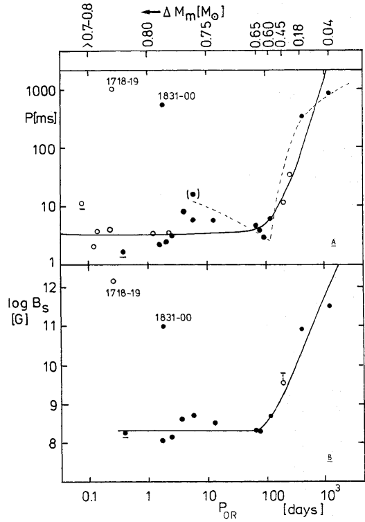
Figure 6.35: The top and the middle panels correspond to spin period, magnetic field vs. orbital period for binary pulsars with circular orbits and low-mass companions. The bottom panel depicts rate of mass transfer vs. the orbital period in low-mass X-ray binaries. $\mbox{$\dot{M}$}_{\rm GR}$ and $\mbox{$\dot{M}$}_{\rm nuc}$ correspond to mass transfers driven by gravitational radiation and by the nuclear evolution of the companion to the neutron star.

In the course of our investigations in this chapter we have seen that there is a positive correlation between the rate of accretion with that of the final field strength, namely, the higher the rate of accretion the higher is the final field. There has already been a mention of such a correlation in connection with the Z and Atoll sources [Hasinger & van der Klis (1989]. It was suggested that the difference between these two classes of sources in regard to their fluctuation spectra is not only due to a difference in the accretion rate but also due to a difference in the magnetic field. And there has been indication from the study of the radiation spectra of these sources that the accretion rate and the magnetic field strength are positively correlated. Recently, ?) on the basis of LMXB spectra and ?) on the basis of the properties of the kilohertz QPOs have indicated the existence of such a correlation. Consider figure [6.35] - the top and the middle panels are taken from ?) and the bottom panel is made using the data from ?). The middle panel shows the variation of the magnetic field with the orbital period for some of the low mass binary pulsars whereas the bottom panel shows the rate of mass accretion with the orbital period in low-mass X-ray binary systems. For longer periods the surface field increases with period. In the bottom panel the rate of accretion shows a similar increase with the orbital period. Therefore we see that for longer orbital periods higher rates of accretion and higher values of surface field are positively correlated. This is another observational indication that for higher rates of accretion the magnetic field strengths tend to be higher.

6.6 conclusions

In this chapter, we have looked at one of the model of magnetic field evolution assuming an initial crustal field configuration to check the consistency with the overall scenario of field evolution for isolated as well as binary pulsars. We find that the model can explain almost all the features that have been observed to date. And our conclusions can be summarized as follows :

• for this model to be consistent with the statistical analyses performed on the isolated pulsars at the most a maximum value of 0.05 for the impurity strength can be allowed;

• HMXBs produce high-field long period pulsars provided the duration of the wind accretion phase is short or the initial current distribution is located at higher densities;

• Relatively low-field ($B\sim 10^{10}$ Gauss) objects near death-line (low-luminosity pulsars) are also predicted from HMXBs;

• LMXBs will produce both high-field long period pulsars as well as low-field short period pulsars inclusive of millisecond pulsars in the later variety; and

• a positive correlation between the rate of accretion and the final field strength is indicated that is supported by observational evidence.

Chapter 7 spin-down induced flux expulsion and its consequences

7.1 introduction

Almost all models of field evolution depend on the mechanism of ohmic decay of the underlying current loops for a permanent decrease in the field strength. It has been mentioned earlier (chapters [3] and [5]) that such ohmic dissipation is possible only if the current loops are situated in the crust where the electrical conductivity is finite. Any flux that may reside in the superconducting core of the star would remain unchanged forever unless this flux is brought out to the crust.

Models that assume an initial core-field configuration, therefore, require a phase of flux expulsion from the core. This expelled flux then undergoes ohmic dissipation in the crust decreasing the surface field strength. One such model uses the spin-evolution to achieve this - that of the ‘spin-down induced flux expulsion’ [Srinivasan (1989, Srinivasan et al. (1990]. The core of the neutron star is believed to contain two superfluids - the neutral neutron superfluid and the charged proton superconductor. Whereas the rotation of the star is supported by creation of vortices in the neutron superfluid, the magnetic flux is sustained by Abrikosov fluxoids in the proton superconductor [Bhattacharya & Srinivasan (1995]. Spinning down of the star requires a decrease in the number of vortices in the superfluid core. Therefore as a result of spin-down the vortices move out towards the core-crust boundary of the star. An inter-pinning between the vortices and the magnetic fluxoids make the fluxoids move outwards too, reducing their number in the core. A decrease in the number of fluxoids in the core reduces the field strength there. The nature of such flux expulsion as a result of spin-evolution has been investigated in detail for both isolated pulsars (undergoing pure dipole spin-down) and for the neutron stars that are members of binaries (undergoing major spin-down in the ‘propeller phase’) [Ding, Cheng, & Chau (1993, Jahan Miri & Bhattacharya (1994, Jahan Miri (1996].

In this chapter we look at the ohmic decay of such expelled field in the crust of an isolated as well as that of an accreting neutron star. Some of the earlier investigations in this direction assumed an uniform ohmic decay time-scale in the crust irrespective of the accretion rate [Jahan Miri & Bhattacharya (1994, Jahan Miri (1996]. The only detailed work in this context has been by ?) where they incorporated the crustal micro-physics into their calculation for the evolution of the expelled field. However this work did not include the material movement that takes place in the crust as a result of accretion. In the present work we incorporate the material movement too and look at the evolution of an expelled field in the crust of an accreting neutron star using the methodology developed in chapter [5].

In the previous chapter we have discussed the overall scenario for the evolution of the neutron star magnetic field - encompassing both isolated neutron stars and those that are members of binary systems. In this chapter we investigate the consequences of the model of ‘spin-down induced flux expulsion’ in the above mentioned systems. We try to judge whether this model, too, is consistent with the overall field scenario and under what conditions. In section [7.2] we shall discuss the results of our computations and conclude in section [7.3].

7.2 results and discussions

Using the methodology developed in chapter [5] we solve the equation [5.16] for an initial flux just expelled at the core-crust boundary due to spin-down. Such an expelled flux is deposited at the bottom of the crust and we start our calculation with such a field configuration. Figure [7.1] shows the distribution of the $g$-function and figure [7.2] the toroidal currents, $J_{\phi}$, assumed at the starting point of our evolution.

Figure 7.1: The initial radial dependence of the $g$-profile, corresponding to an expelled flux, centred at $x=0.925$, with a width $\delta x$ = 0.006; where $x$ is the fractional radius $r/R$.

Figure 7.2: The initial radial dependence of the $\phi$-component of the corresponding current configuration.

7.2.1 ohmic decay in isolated pulsars

The cause of flux expulsion is the spinning down of the pulsar. Therefore, for isolated pulsars too, experiencing a pure dipole slow-down, there would be some flux expulsion. The extent of such flux expulsion has been worked out by ?) and it has been shown there that the flux expulsion is most effective for pulsars with large values of magnetic field strength. Before discussing the field evolution in neutron stars in binary systems, we first look at the ohmic decay of such an expelled field in isolated pulsars. We consider the isolated neutron star to undergo standard cooling, in order to find the maximum extent of field reduction in this case. But by the time significant flux-expulsion is achieved, the crustal temperature goes down to very low values for an isolated neutron star. In such a situation the conductivity would be mainly determined by the scattering of the conduction electrons by the impurities. To see the effect of that we have considered here several values of impurity strength $Q$ (see section [2.4] for details).

Figure 7.3: Pure ohmic diffusion of the $g$-profile plotted in figure [7.1] for $\tau\sim 10^{9}$ yrs, with $Q$ = 0.1, in a neutron star with standard cooling. The curves are shown for intermediate times with no discernible change in the value at the surface ($x$ = 1).

Figure 7.4: Same as figure [7.3] with $Q$ = 0.2. The profiles show an initial increase and a substantial decrease in the surface value over a time-scale of $10^{9}$ years.

Figure 7.5: The evolution of the surface magnetic field due to pure diffusion of an expelled flux corresponding to the evolution of the $g$-profile plotted in the previous figures. The dotted and the solid curves correspond to $Q$ = 0.0, 0.1, 0.2, 0.3 and 0.4 respectively.

In figures [7.3] and [7.4] we have plotted the time evolution of the $g$-profile for two values of the impurity strength. In figure [7.5] the corresponding evolution of the surface fields for five values of the impurity strength are plotted. It is seen very clearly that the surface field actually increases when the expelled flux diffuses outwards before finally decaying down to smaller values. It is to be noted that even for a very large value of the impurity strength ($Q$ = 0.4) the surface field shows significant decay only over a time-scale of $\sim 10^{9}$ years. The active lifetime of an isolated radio pulsar is $\raisebox{-1.29167pt}{\mbox{$\stackrel{{\scriptstyle<}}{{{}_{\sim}}}\,$}}10^{8}$ years. Therefore, an isolated radio pulsar would experience little field decay over its active lifetime, consistent with the indications from statistical analyses. So we conclude that with an expelled flux there is provision for large values of $Q$ to exist in the crust of the neutron star. In fact, we shall see later that in this model large $Q$ is a necessary requirement for millisecond pulsar generation.

7.2.2 field evolution with accretion

Figure 7.6: Evolution of the surface magnetic field for an expelled flux. The curves 1 to 5 correspond to $\mbox{$\dot{M}$}=10^{-13},10^{-12},10^{-11},10^{-10},10^{-9}$ M_⊙ yr^-1. All curves correspond to $Q$ = 0.0.

Figure 7.7: Evolution of the surface magnetic field for an expelled flux. The different curves from top to bottom correspond to $Q$ = 0, 0.1, 0.2, 0.3 and 0.4 respectively. All curves correspond to $\mbox{$\dot{M}$}=10^{-10}$ M_⊙ yr^-1.

Before looking into the nature of field evolution in various binary systems, we first investigate the evolution of the surface field under accretion, assuming the $g$-profile plotted in figure [7.1] as the initial condition. In figure [7.6] we plot the evolution of the surface field for different values of the accretion rate and in figure [7.7] we plot the evolution for different values of the impurity strength. We find that the field strengths go down by about only one and a half order of magnitude even for a fairly large value of the impurity strength. Therefore, even higher values of impurity strength will be required for a larger reduction in the field strength. We shall see later that for certain cases the required impurity strength is much larger than that considered by us here (we have considered a maximum $Q$ value of 0.4) to achieve millisecond pulsar field values. The characteristic features of field evolution are then as follows.

1. An initial rapid decay (neglecting the early increase) is followed by a slow down and an eventual freezing.

2. The onset of ‘freezing’ is faster with higher rates of accretion, i.e., at higher values of crustal temperature.

3. Lower final ‘frozen’ fields are achieved for lower rates of accretion.

4. To achieve a significant reduction in the field strength, very large values of the impurity strength are required.

It is clear from these features that the general nature of field evolution in the case of an expelled flux is qualitatively similar to that in the case of an initial crustal flux. This indicates that the behaviour of the field evolution in different kinds of binaries will again be similar to what we have found in the case of an initial crustal flux, discussed in chapter [6].

7.2.3 field evolution in binaries

In section [6.3] we have outlined the three phase of binary evolution, namely - the isolated, the wind and the Roche-contact phase. In the wind phase there are two distinct possibilities of interaction between the neutron star and its main sequence companion. If the system is in the ‘propeller phase’ then there is no mass accretion. But the importance of this phase is that the star rapidly slows down to very long periods and as a result a significant flux-expulsion is achieved. From the point of view of flux expulsion, therefore, we assume the flux to be completely contained within the superconducting core (neglecting the small flux-expulsion caused by the dipole spin-down in the isolated phase) prior to this phase. Therefore, the ohmic decay of this flux will take place only after this phase is over - that is in the phase of wind-accretion and most-importantly in the phase of Roche-contact. It has already been noted that, in case of low mass X-ray binaries, it is not very clear as to how long the phase of wind-accretion lasts or whether such a phase is at all realized after the ‘propeller phase’ is over. Therefore, in our calculations we have considered cases with and without a phase of wind accretion, as before.

7.2.3.1 high mass binaries

Figure 7.8: Evolution of the surface magnetic field in high mass X-ray binaries for four values of wind accretion rate. The curves 1 to 5 correspond to $\mbox{$\dot{M}$}=10^{-14},10^{-13},10^{-12},10^{-11},10^{-10}$ M_⊙ yr^-1. Though here curves 1 and 2 are indistinguishable. All curves correspond to $Q$ = 0.0.

Figure 7.9: Same as figure [7.8] with $Q$ = 0.04.

Figure 7.10: Same as figure [7.8] with the Roche-contact phase expanded. The solid and the dotted curves correspond to curves 1 and 2 in figure [7.8].

Figures [7.8] and [7.9] show the evolution of the surface field in high mass X-ray binaries for different values of the impurity strength in the crust. The parameters for the high mass X-ray binary evolution are as before. The surface field shows a clear initial increase followed by a sharp decay. The decay in the Roche-contact phase is very small and is almost invisible in the above-mentioned plots. In figure [7.10] we have expanded the Roche-phase corresponding to the figure [7.8] to highlight this phase. For the impurity strengths considered by us, the field decreases by about an order of magnitude.

7.2.3.2 low mass binaries

Figure 7.11: Evolution of the surface magnetic field in low mass X-ray binaries for two values of the wind accretion rate. The curves 1 to 5 correspond to $Q$ = 0.0, 0.01, 0.02, 0.03 and 0.04 respectively. All curves correspond to a wind accretion rate of $\mbox{$\dot{M}$}=10^{-16}$ M_⊙ yr^-1.

Figure 7.12: Same as figure [7.11] with a wind accretion rate of $\mbox{$\dot{M}$}=10^{-14}$ M_⊙ yr^-1.

Figure 7.13: Same as figure [7.11] with the Roche-contact phase expanded. The solid and the dotted curves correspond to accretion rates of $\mbox{$\dot{M}$}=10^{-10},10^{-9}$ M_⊙ yr^-1in the Roche contact phase.

Figure 7.14: Same as figure [7.12] with the Roche-contact phase expanded.The solid and the dotted curves correspond to accretion rates of $\mbox{$\dot{M}$}=10^{-10},10^{-9}$ M_⊙ yr^-1in the Roche contact phase.

Figure 7.15: Evolution of the surface magnetic field in low mass X-ray binaries without a phase of wind accretion. The set of curves (a) and (b) correspond to accretion rates of $\mbox{$\dot{M}$}=10^{-9},10^{-10}$ M_⊙ yr^-1in the Roche contact phase. Individual curves in each set correspond to $Q$ = 0.0, 0.1, 0.2, 0.3 and 0.4 respectively, the upper curves being for the lower values of $Q$.

Figures [7.11] and [7.12] show the evolution of the surface field in the low mass X-ray binaries; for different values of the impurity concentration in the crust. The two figures correspond to two different values of accretion rate in the wind phase. It should be noted that this difference in the wind accretion rate does not manifest itself in either the nature of the field evolution or the final field strengths. However, a difference in the accretion rate in the Roche-contact phase shows up very clearly in figures [7.13] and [7.14] where the Roche-contact phases, corresponding to the figures [7.11] and [7.12], have been expanded. Comparing the different curves (for different values of the impurity parameter) we see that a large value of impurity strength gives rise to a rapid decay and therefore a low value of the final surface field.

In figure [7.15] we have plotted the evolution of the surface field assuming the wind accretion phase to be absent. Once again we find that for higher rates of accretion higher final field values are obtained. It should be noted here that the final field values obtained now are only about an order and a half of magnitude lower than the original surface field strengths. Even though the impurity strengths assumed now are much higher than those assumed when we investigated the field evolution in low mass X-ray binaries with a phase of wind-accretion. In absence of a prior phase of wind accretion the flux does not have enough time to diffuse out to low density regions when the Roche-contact is established. Therefore here the role of accretion, in the Roche-contact phase, is mainly to push the currents in rather than to enhance ohmic decay rate. Evidently, much larger impurity strength is required to be assumed in order that the final field values could be reduced by three to four orders of magnitude. Unfortunately, due to numerical instabilities it becomes very difficult to explore situations with even higher values of $Q$. But the above-mentioned figure clearly establishes a trend as to how the final field values behave with $Q$ and it is evident that we need $Q$ values much larger than those considered here to get down to millisecond pulsar field strengths.

The most important point to note here is the fact that again, similar to an initial crustal field configuration, the amount of field decay is much larger than that achieved in the case of high mass X-ray binaries. Although, in low mass X-ray binaries with higher values of impurity strength the surface field does go down by three to four orders of magnitude from its original value, the final field strength could remain fairly large if the impurity strength is small. But if the wind-accretion phase is absent in these systems then to achieve large amount of reduction in the field strengths much larger value of the impurity strength will be required. Therefore, the ‘spin-down induced flux expulsion model’ will be consistent with the overall scenario of field evolution and in particular millisecond pulsars can be produced in low mass X-ray binaries provided the impurity strength in the crust of the neutron stars is assumed to be extremely large.

7.3 conclusions

In this chapter we have investigated the consequences of ‘spin-down induced flux expulsion’. So far, the general nature of field evolution seem to fit the overall scenario. The nature of field evolution is quite similar to that in case of a purely crustal model of field evolution though the details differ. Most significantly, this model has the requirement of large values of the impurity strength $Q$ in direct contrast to the crustal model. To summarize then :

• The field in isolated neutron stars do not undergo any significant decay, over the active lifetime of the pulsar, conforming with the statistical analyses.

• The field values in the high mass X-ray binaries can reaming fairly large for a moderate range of impurity strength.

• A reduction of three to four orders of magnitude in the field strength can be achieved in the low mass X-ray binaries provided the impurity strength is as large as 0.5.

• If the wind accretion phase is absent then to achieve millisecond pulsar field values, impurity strength in excess of unity is required.

Chapter 8 conclusions

In this final chapter we shall summarize the main conclusions of our investigations. For our work we have drawn upon many results which are not entirely free of uncertainties. We shall also mention here such uncertainties that are likely to affect our results. And lastly we shall indicate the future directions of work in this context.

1. Generic Features of Field Evolution in the Crust – In this thesis we have mainly investigated two models of field evolution that of an initial crustal current supporting the field and the model of spin-down induced flux expulsion. The qualitative features of field evolution are same for both the models. We have also looked at the effect of diamagnetic screening in an accreting neutron star. The nature of this screening is such that an assumption regarding a particular model of field configuration is unnecessary and the results of this investigation are model-independent. Therefore, we have the following general conclusions regarding the nature of field evolution in the crust.

   • Pure Ohmic Decay in Isolated Neutron Stars :

     1. A slow cooling of the star gives rise to a fast decay and consequent low final field. The opposite happens in case of an accelerated cooling.

     2. An initial crustal current distribution concentrated at lower densities again gives rise to faster decay and low final surface field. Whereas if the current is located at higher densities the decay is slow resulting in a higher final surface field.

     3. A large value of impurity strength implies a rapid decay and low final field. If the crust behaves more like a pure crystal the decay slows down considerably.

   • Accretion-Induced Field Decay in Accreting Neutron Stars :

     1. In an accreting neutron star the field undergoes an initial rapid decay, followed by slow down and an eventual freezing.

     2. A positive correlation between the rate of accretion and the final field strength is observed, giving rise to higher final saturation field strengths for higher rates of accretion.

     3. An expected screening of the surface field by the diamagnetic accreting material is rendered ineffective by the interchange instabilities in the liquid surface layers of the star.

2. Nature of Field and Spin Evolution in Real Systems – In the next phase of our investigation we have applied the models of field evolution to real systems - isolated neutron stars as well as to those in binaries. The paradigm of field evolution that have emerged out of various observations, statistical analyses and theoretical expectations have been summarized in the following flow-diagram. The arrows indicate the expected evolutionary link between X-ray binaries and binary radio pulsars. The following table summarizes the results of our investigations.

   

   Evolution of a Purely Crustal Field
   Our Results
   system	final field and period	comment
   isolated	high field, long period	no significant field decay
   radio pulsars		in $10^{9}$  years
   HMXB	high field, long period	high-mass binary pulsars
   		and solitary counterparts
   	low field, long period	not active as pulsars
   LMXB	high field, long period	high field low-mass binary pulsars
   		and solitary counterparts
   	low field, short period	low field low-mass binary pulsars
   		and solitary counterparts,
   		millisecond pulsars

   It is evident that the results obtained from the field evolution models agree well with the observational paradigm. The nature of field evolution is similar for the model of spin-down induced flux expulsion. Though there is one major difference. To produce millisecond pulsars in LMXBs in spin-down induced flux expulsion model very large values of impurities are required. This makes the surface field go down to very low values in $10^{9}$ years in isolated pulsars in contrast to a purely crustal model.

3. Ranges of Physical Parameters – In the following table we summarize the constraints on various physical parameters in the field evolution models placed by the requirement to match observed properties in a variety of systems. The parameters discussed here are - the density at which the initial crustal current distribution is located ($\rho_{0}$), the impurity strength in the crust ($Q$), the duration of wind-accretion phase in different binary systems and the rate of accretion in the Roche-contact phase for LMXBs.

   Constraints on Physical Parameters
   parameter	model	system	requirement	parameter range
   $\rho_{0}$	crustal	hmxb	high field	high $\rho_{0}$
   $Q$	crustal	isolated	no field decay	$Q\raisebox{-1.29167pt}{\mbox{$\stackrel{{\scriptstyle<}}{{{}_{\sim}}}\,$}}0.01$ for
   		radio pulsar	over active	standard cooling,
   			pulsar life-time	$Q\raisebox{-1.29167pt}{\mbox{$\stackrel{{\scriptstyle<}}{{{}_{\sim}}}\,$}}0.05$ for
   				accelerated cooling
   	core	LMXB	millisecond pulsar	$Q\raisebox{-1.29167pt}{\mbox{$\stackrel{{\scriptstyle>}}{{{}_{\sim}}}\,$}}0.05$ with
   			generation	wind accretion,
   				$Q>>1$ without
   				wind accretion
   duration of	crustal	HMXB	high field	short
   wind accretion
   $\dot{M}$ in	crustal	LMXB	high field	Eddington rate
   Roche-phase

4. Uncertainties – The results and conclusions stated above suffer from a number of uncertainties regarding the micro-physics of the neutron star, as listed below.

   • Thermal Behaviour -

     1. Isolated Phase - The present date can be made to fit scenarios with both a slow or an accelerated cooling. Hence it is not clear which is the correct cooling behaviour of an isolated neutron star.

     2. Accreting Phase - the crustal temperature corresponding to a given rate of accretion has not been determined with any certainty. Also, the existing results are limited in their scope and there is no agreement between various authors.

     3. Post-Accretion Phase - No calculation exists for the thermal behaviour of this phase at all.

   • Transport Properties - There are several factors, the effects of which have not been incorporated yet, namely those of

     1. the change in the chemical composition due to a) accretion and b) spin-down; and

     2. the dislocations, defects etc. of the crustal lattice.

   • Equation of State - Apart from the uncertainties already existent for a cold equation of state, the change in the chemical composition due to accretion introduces change in the equation of state and hence in a) the structure of the star and its b) transport properties.

   • All of our investigation has been based on an assumption of a pure dipolar model for the magnetic field. The validity of these results requires to be checked by including higher order multi-poles for the field.

5. Future Directions – One of the most important questions in the context of the evolution of magnetic fields in neutron stars is regarding the models of field generation (and therefore of the internal field configuration). There is no consensus as to which one is actually realized. Our calculations clearly point out that the models have very different requirements for the impurity strength in the crust. Possible ways of resolving this dilemma then could be the following.

   • Theoretical - A better many-body calculations may determine the state of matter in the crust accurately in regard to its impurity content.

   • Observational Prediction - An old solitary radio pulsar will have a very low field if the impurity content of the crust is very large. The detection of such a pulsar accreting matter from the interstellar matter will therefore immediately indicate the impurity content of the crust. The results of our investigation clearly indicate that the both the models place very stringent limits on the impurity strength and the limits from the different models are quite incompatible. Therefore such an observation will immediately determine the viability of one model or the other - predictably providing an answer to this question.

Bibliography

- Ainsworth, Wambach, & Pines (1989 Ainsworth T. L., Wambach J., Pines D., 1989, Phys. Lett. B, 222, 173
- Alpar (1991 Alpar M. A., 1991, in NATO ASIC Proc. 344: Neutron Stars, p. 49
- Alpar et al. (1982 Alpar M. A., Cheng A. F., Ruderman M. A., Shaham J., 1982, Nat, 300, 728
- Ashcroft & Mermin (1979 Ashcroft N. W., Mermin N. D., 1979, Solid State Physics. Thomson Learning, London
- Baade & Zwicky (1934 Baade W., Zwicky F., 1934, Proceedings of the National Academy of Science, 20, 254
- Backer et al. (1982 Backer D. C., Kulkarni S. R., Heiles C., Davis M. M., Goss W. M., 1982, Nat, 300, 615
- Baiko & Yakovlev (1995 Baiko D. A., Yakovlev D. G., 1995, Astronomy Letters, 21, 702
- Bailes (1996 Bailes M., 1996, in ASP Conf. Ser. 105: IAU Colloq. 160: Pulsars: Problems and Progress, p. 3
- Baym, Bethe, & Pethick (1971 Baym G., Bethe H. A., Pethick C. J., 1971, Nucl. Phys. A, 175, 225
- Baym et al. (1969 Baym G., Pethick C., Pines D., Ruderman M., 1969, Nat, 224, 872
- Baym, Pethick, & Sutherland (1971 Baym G., Pethick C., Sutherland P., 1971, ApJ, 170, 299
- Baym, Pethick, & Pines (1969 Baym G., Pethick C. J., Pines D., 1969, Nat, 224, 673
- Bhattacharya (1995a Bhattacharya D., 1995a, in Alpar M. A., Kiziloglu U., van Paradijs J., ed, The Lives of the Neutron Stars. Kluwer Academic Publishers, Dordrecht, p. 153
- Bhattacharya (1995b Bhattacharya D., 1995b, JA&A, 16, 217
- Bhattacharya (1996a Bhattacharya D., 1996a, in IAU Symp. 165: Compact Stars in Binaries, p. 243
- Bhattacharya (1996b Bhattacharya D., 1996b, in Astronomical Society of the Pacific Conference Series, Vol. 105, Johnston S., Walker M. A., Bailes M., ed, IAU Colloq. 160: Pulsars: Problems and Progress. ASP, San Francisco, p. 547
- Bhattacharya (1996c Bhattacharya D., 1996c, in Astronomical Society of the Pacific Conference Series, Vol. 105, Johnston S., Walker M. A., Bailes M., ed, IAU Colloq. 160: Pulsars: Problems and Progress, p. 547
- Bhattacharya & Datta (1996 Bhattacharya D., Datta B., 1996, MNRAS, 282, 1059
- Bhattacharya & Srinivasan (1986 Bhattacharya D., Srinivasan G., 1986, Curr. Sc., 55, 327
- Bhattacharya & Srinivasan (1991 Bhattacharya D., Srinivasan G., 1991, JA&A, 12, 17
- Bhattacharya & Srinivasan (1995 Bhattacharya D., Srinivasan G., 1995, in Lewin W. H. G., van Paradijs J., van den Heuvel E. P. J., ed, X-ray binaries, p. 495 - 522. Cambridge University Press, p. 495
- Bhattacharya & van den Heuvel (1991 Bhattacharya D., van den Heuvel E. P. J., 1991, Phys. Rep., 203, 1
- Bhattacharya et al. (1992 Bhattacharya D., Wijers R. A. M. J., Hartman J. W., Verbunt F., 1992, A&A, 254, 198
- Bildsten & Cutler (1995 Bildsten L., Cutler C., 1995, ApJ, 449, 800
- Bisnovatyi-Kogan & Komberg (1974 Bisnovatyi-Kogan G. S., Komberg B. V., 1974, Soviet Astronomy, 18, 217
- Blandford, Applegate, & Hernquist (1983 Blandford R. D., Applegate J. H., Hernquist L., 1983, MNRAS, 204, 1025
- Blandford, Decampli, & Kiönigl (1979 Blandford R. D., Decampli W. M., Kiönigl A., 1979, BAAS, 11, 703
- Callanan et al. (1989 Callanan P. J., Charles P. A., Hassal B. J. M., Machin G., Mason K. O., Naylor T., Smale A. P., van Paradijs J., 1989, MNRAS, 238, 25P
- Camilo et al. (1996 Camilo F., Nice D. J., Shrauner J. A., Taylor J. H., 1996, ApJ, 469, 819
- Chabrier, Potekhin, & Yakovlev (1997 Chabrier G., Potekhin A. Y., Yakovlev D. G., 1997, ApJ, 477, L99
- Chandrasekhar (1931 Chandrasekhar S., 1931, Phil. Mag., 11, 592
- Chen & Ruderman (1993 Chen K., Ruderman M., 1993, ApJ, 402, 264
- Cheng & Dai (1997 Cheng K. S., Dai Z. G., 1997, ApJ, 476, L39
- Cordes & Chernoff (1997 Cordes J. M., Chernoff D. F., 1997, ApJ, 482, 971
- Cordes et al. (1990 Cordes J. M., Wolszczan A., Dewey R. J., Blaskiewicz M., Stinebring D. R., 1990, ApJ, 349, 245
- Datta, Thampan, & Bhattacharya (1995 Datta B., Thampan A. V., Bhattacharya D., 1995, JA&A, 16, 375
- Ding, Cheng, & Chau (1993 Ding K. Y., Cheng K. S., Chau H. F., 1993, ApJ, 408, 167
- Feynman, Metropolis, & Teller (1949 Feynman R. P., Metropolis N., Teller E., 1949, Phys. Rev., 75, 1561
- Friedman & Pandharipande (1981 Friedman B., Pandharipande V. R., 1981, Nucl. Phys. A, 361, 502
- Fruchter, Stinebring, & Taylor (1988 Fruchter A. S., Stinebring D. R., Taylor J. H., 1988, Nat, 333, 237
- Fujimoto et al. (1984 Fujimoto M. Y., Hanawa T., Iben I., Richardson M. B., 1984, ApJ, 278, 813
- Geppert & Urpin (1994 Geppert U., Urpin V., 1994, MNRAS, 271, 490
- Geppert, Urpin, & Konenkov (1996 Geppert U., Urpin V., Konenkov D., 1996, A&A, 307, 807
- Geppert & Wiebicke (1991 Geppert U., Wiebicke H. J., 1991, A&AS, 87, 217
- Geppert & Wiebicke (1995 Geppert U., Wiebicke H. J., 1995, A&A, 300, 429
- Ginzburg (1964 Ginzburg V. L., 1964, Soviet Physics Doklady, 9, 329
- Ginzburg & Kirzhnits (1964 Ginzburg V. L., Kirzhnits D. A., 1964, Zh. Eksp. Teor. Fiz., 47, 2006
- Gold (1968 Gold T., 1968, Nat, 218, 731
- Gold (1969 Gold T., 1969, Nat, 221, 25
- Gudmundsson, Pethick, & Epstein (1982 Gudmundsson E. H., Pethick C. J., Epstein R. I., 1982, ApJ, 259, L19
- Gudmundsson, Pethick, & Epstein (1983 Gudmundsson E. H., Pethick C. J., Epstein R. I., 1983, ApJ, 272, 286
- Gunn & Ostriker (1969 Gunn J. E., Ostriker J. P., 1969, Nat, 221, 454
- Gunn & Ostriker (1970 Gunn J. E., Ostriker J. P., 1970, ApJ, 160, 979
- Haensel, Zdunik, & Dobaczewski (1989 Haensel P., Zdunik J. L., Dobaczewski J., 1989, A&A, 222, 353
- Hameury et al. (1983 Hameury J. M., Bonazzola S., Heyvaerts J., Lasota J. P., 1983, A&A, 128, 369
- Hanawa (1992 Hanawa T., 1992, in Structure and Evolution of Neutron Stars, p. 221
- Hansen & Phinney (1997 Hansen B. M. S., Phinney E. S., 1997, MNRAS, 291, 569
- Hartman et al. (1997 Hartman J. W., Bhattacharya D., Wijers R., Verbunt F., 1997, A&A, 322, 477
- Hasinger & van der Klis (1989 Hasinger G., van der Klis M., 1989, A&A, 225, 79
- Hewish et al. (1968 Hewish A., Bell S. J., Pilkington J. D., Scott P. F., Collins R. A., 1968, Nat, 217, 709
- Hulse & Taylor (1975 Hulse R. A., Taylor J. H., 1975, ApJ, 195, L51
- Itoh (1994 Itoh N., 1994, in IAU Colloq. 147: The Equation of State in Astrophysics, p. 394
- Itoh, Hayashi, & Kohyama (1993 Itoh N., Hayashi H., Kohyama Y., 1993, ApJ, 418, 405
- Itoh et al. (1984 Itoh N., Kohyama Y., Matsumoto N., Seki M., 1984, ApJ, 285, 758
- Iwamoto et al. (1995 Iwamoto N., Qin L., Fukugita M., Tsuruta S., 1995, Phys. Rev. D, 51, 348
- Jackson (1975 Jackson J. D., 1975, Classical Electrodynamics. John Wiley & Sons Incorporated
- Jahan Miri (1996 Jahan Miri M., 1996, MNRAS, 283, 1214
- Jahan Miri & Bhattacharya (1994 Jahan Miri M., Bhattacharya D., 1994, MNRAS, 269, 455
- King et al. (1995 King A. R., Frank J., Kolb U., Ritter H., 1995, ApJ, 444, L37
- Konar & Bhattacharya (1997 Konar S., Bhattacharya D., 1997, MNRAS, 284, 311
- Konar, Bhattacharya, & Urpin (1995 Konar S., Bhattacharya D., Urpin V., 1995, JA&A, 16, 249
- Kulkarni (1986 Kulkarni S. R., 1986, ApJ, 306, L85
- Kulkarni, Djorgovski, & Klemola (1991 Kulkarni S. R., Djorgovski S., Klemola A. R., 1991, ApJ, 367, 221
- Kulkarni & Narayan (1988 Kulkarni S. R., Narayan R., 1988, ApJ, 335, 755
- Lattimer (1992 Lattimer J. M., 1992, in Pines D., Tamagaki R., Tsuruta S., ed, Structure and Evolution of Neutron Stars. Addison Wesley, p. 50
- Lattimer et al. (1991 Lattimer J. M., Prakash M., Pethick C. J., Haensel P., 1991, Phys. Rev. Lett., 66, 2701
- Lorenz, Ravenhall, & Pethick (1993 Lorenz C. P., Ravenhall D. G., Pethick C. J., 1993, Phys. Rev. Lett., 70, 379
- Lorimer (1994 Lorimer D., 1994, Ph.D. thesis, The University of Manchester
- Lorimer (1995 Lorimer D. R., 1995, MNRAS, 274, 300
- Lyne, Anderson, & Salter (1982 Lyne A. G., Anderson B., Salter M. J., 1982, MNRAS, 201, 503
- Manchester & Taylor (1977 Manchester R. N., Taylor J. H., 1977, Pulsars. W. H. Freeman and Company, San Fransisco
- Miralda-Escude, Paczynski, & Haensel (1990 Miralda-Escude J., Paczynski B., Haensel P., 1990, ApJ, 362, 572
- Negele & Vautherin (1973 Negele J. W., Vautherin D., 1973, Nucl. Phys. A, 207, 298
- Nicastro & Johnston (1995 Nicastro L., Johnston S., 1995, MNRAS, 273, 122
- Nice & Taylor (1995 Nice D. J., Taylor J. H., 1995, ApJ, 441, 429
- Oppenheimer & Volkoff (1939 Oppenheimer J. R., Volkoff G. M., 1939, Phys. Rev., 55, 374
- Ostriker & Gunn (1969 Ostriker J. P., Gunn J. E., 1969, ApJ, 157, 1395
- Pacini (1967 Pacini F., 1967, Nat, 216, 567
- Pacini (1968 Pacini F., 1968, Nat, 219, 145
- Page (1998 Page D., 1998, in Shibazaki N., ed, Neutron Stars and Pulsars: Thirty Years after the Discovery. Universal Academy Press, Tokyo, p. 183
- Pandharipande, Pines, & Smith (1976 Pandharipande V. R., Pines D., Smith R. A., 1976, ApJ, 208, 550
- Pavlov et al. (1996 Pavlov G. G., Zavlin V. E., Truemper J., Neuhaeuser R., 1996, ApJ, 472, L33
- Pethick (1992 Pethick C. J., 1992, Rev. Mod. Phys., 64, 1133
- Pethick & Ravenhall (1992 Pethick C. J., Ravenhall D. G., 1992, Royal Society of London Philosophical Transactions Series A, 341, 17
- Pethick & Thorsson (1994 Pethick C. J., Thorsson V., 1994, Phys. Rev. Lett., 72, 1964
- Pines (1991 Pines D., 1991, in Ventura J., Pines D., ed, NATO ASIC Proc. 344: Neutron Stars. Kluwer Academic Publishers, Dordrecht, p. 57
- Pines & Alpar (1992 Pines D., Alpar M. A., 1992, in Pines D., Tamagaki R., Tsuruta S., ed, Structure and Evolution of Neutron Stars. Addison Wesley, p. 7
- Potekhin, Chabrier, & Yakovlev (1997 Potekhin A. Y., Chabrier G., Yakovlev D. G., 1997, A&A, 323, 415
- Prakash (1994 Prakash M., 1994, Phys. Rep., 242, 297
- Prakash et al. (1992 Prakash M., Prakash M., Lattimer J. M., Pethick C. J., 1992, ApJ, 390, L77
- Press et al. (1988 Press W. H., Flannery B. P., Teukolsky S. A., Vetterling W. T., 1988, Numerical Recipes. Cambridge University Press
- Press et al. (1992 Press W. H., Teukolsky S. A., Vetterling W. T., Flannery B. P., 1992, Numerical recipes in FORTRAN. The art of scientific computing
- Psaltis & Lamb (1998 Psaltis D., Lamb F. K., 1998, in Shibazaki N., ed, Neutron Stars and Pulsars: Thirty Years after the Discovery, p. 179
- Radhakrishnan & Srinivasan (1982 Radhakrishnan V., Srinivasan G., 1982, Curr. Sc., 51, 1096
- Ramachandran & Bhattacharya (1997 Ramachandran R., Bhattacharya D., 1997, MNRAS, 288, 565
- Romani (1990 Romani R. W., 1990, Nat, 347, 741
- Romani (1995 Romani R. W., 1995, in van Riper K., Epstein R., Ho C., ed, Isolated Pulsars. Cambridge University Press, p. 75
- Ruderman (1991a Ruderman M., 1991a, ApJ, 366, 261
- Ruderman (1991b Ruderman M., 1991b, ApJ, 382, 587
- Ruderman (1995 Ruderman M., 1995, JA&A, 16, 207
- Ruderman et al. (1989 Ruderman M., Shaham J., Tavani M., Eichler D., 1989, ApJ, 343, 292
- Ruderman & Sutherland (1973 Ruderman M. A., Sutherland P. G., 1973, Nat, 246, 93
- Ruderman (1991c Ruderman R., 1991c, ApJ, 382, 576
- Sang & Chanmugam (1987 Sang Y., Chanmugam G., 1987, ApJ, 323, L61
- Savonije (1978 Savonije G. J., 1978, A&A, 62, 317
- Schaab et al. (1997 Schaab C., Voskresensky D., Sedrakian A. D., Weber F., Weigel M. K., 1997, A&A, 321, 591
- Shapiro & Teukolsky (1983 Shapiro S. L., Teukolsky S. A., 1983, Black Holes, White Dwarfs and Neutron Stars. John Wiley & Sons, New York
- Shibanov & Yakovlev (1996 Shibanov Y. A., Yakovlev D. G., 1996, A&A, 309, 171
- Shibazaki et al. (1989 Shibazaki N., Murakami T., Shaham J., Nomoto K., 1989, Nat, 342, 656
- Slattery, Doolen, & Dewitt (1982 Slattery W. L., Doolen G. D., Dewitt H. E., 1982, Phys. Rev. A, 26, 2255
- Spruit (1983 Spruit H. C., 1983, in Stenflo J. O., ed, Solar and Stellar Magnetic Fields : Origins and Coronal Effects, IAU Symposium No. 102. D. Reidel Publishing Company
- Srinivasan (1989 Srinivasan G., 1989, A&AR, 1, 209
- Srinivasan (1995 Srinivasan G., 1995, in Benz A. O., Courvoisier T. J.-L., ed, Saas-Fee Advanced Course 25: Stellar Remnants. Springer, Berlin, p. 97
- Srinivasan et al. (1990 Srinivasan G., Bhattacharya D., Muslimov A. G., Tsygan A. J., 1990, Curr. Sc., 59, 31
- Srinivasan & van den Heuvel (1982 Srinivasan G., van den Heuvel E. P. J., 1982, A&A, 108, 143
- Taam & van de Heuvel (1986 Taam R. E., van de Heuvel E. P. J., 1986, ApJ, 305, 235
- Tatsumi & Muto (1992 Tatsumi T., Muto T., 1992, in Pines D., Tamagaki R., Tsuruta S., ed, Structure and Evolution of Neutron Stars. Addison Wesley, p. 178
- Truemper et al. (1978 Truemper J., Pietsch W., Reppin C., Voges W., Staubert R., Kendziorra E., 1978, ApJ, 219, L105
- Urpin & Geppert (1995 Urpin V., Geppert U., 1995, MNRAS, 275, 1117
- Urpin & Geppert (1996 Urpin V., Geppert U., 1996, MNRAS, 278, 471
- Urpin, Levshakov, & Iakovlev (1986 Urpin V. A., Levshakov S. A., Iakovlev D. G., 1986, MNRAS, 219, 703
- Urpin & Muslimov (1992a Urpin V. A., Muslimov A. G., 1992a, MNRAS, 256, 261
- Urpin & Muslimov (1992b Urpin V. A., Muslimov A. G., 1992b, Soviet Astronomy, 36, 530
- van den Heuvel, van Paradijs, & Taam (1986 van den Heuvel E. P., van Paradijs J. A., Taam R. E., 1986, Nat, 322, 153
- van den Heuvel (1995 van den Heuvel E. P. J., 1995, JA&A, 16, 255
- van den Heuvel & Bitzaraki (1995 van den Heuvel E. P. J., Bitzaraki O., 1995, A&A, 297, L41
- van Riper (1991a van Riper K. A., 1991a, ApJS, 75, 449
- van Riper (1991b van Riper K. A., 1991b, ApJ, 372, 251
- Verbunt (1990 Verbunt F., 1990, in Kundt W., ed, NATO ASIC Proc. 306: Neutron Stars and Their Birth Events, p. 179
- Verbunt & van den Heuvel (1995 Verbunt F., van den Heuvel E. P. J., 1995, in Lewin W. H. G., van Paradijs J., van den Heuvel E. P. J., ed, X-Ray Binaries. Cambridge University Press, p. 457
- Verbunt, Wijers, & Burm (1990 Verbunt F., Wijers R. A. M. J., Burm H. M. G., 1990, A&A, 234, 195
- Wakatsuki et al. (1992 Wakatsuki S., Hikita A., Sato N., Itoh N., 1992, ApJ, 392, 628
- Wendell, van Horn, & Sargent (1987 Wendell C. E., van Horn H. M., Sargent D., 1987, ApJ, 313, 284
- White & Zhang (1997 White N. E., Zhang W., 1997, ApJ, 490, L87
- Wiebicke & Geppert (1991 Wiebicke H. J., Geppert U., 1991, A&A, 245, 331
- Wiebicke & Geppert (1992 Wiebicke H. J., Geppert U., 1992, A&A, 262, 125
- Wiebicke & Geppert (1995 Wiebicke H. J., Geppert U., 1995, A&A, 294, 303
- Wiebicke & Geppert (1996 Wiebicke H. J., Geppert U., 1996, A&A, 309, 203
- Wijers (1997 Wijers R. A. M. J., 1997, MNRAS, 287, 607
- Wiringa, Fiks, & Fabrocini (1988 Wiringa R. B., Fiks V., Fabrocini A., 1988, Phys. Rev. C, 38, 1010
- Wolszczan (1994 Wolszczan A., 1994, Science, 264, 538
- Woltjer (1964 Woltjer L., 1964, ApJ, 140, 1309
- Woosley & Wallace (1982 Woosley S. E., Wallace R. K., 1982, ApJ, 258, 716
- Yakovlev & Urpin (1980 Yakovlev D. G., Urpin V. A., 1980, Soviet Astronomy, 24, 303
- Zdunik et al. (1992 Zdunik J. L., Haensel P., Paczynski B., Miralda-Escude J., 1992, ApJ, 384, 129
- Zhang (1998 Zhang C. M., 1998, A&A, 330, 195
- Zhang, Wu, & Yang (1994 Zhang C.-M., Wu X.-J., Yang G.-C., 1994, A&A, 283, 889