Multi-terminal Thermoelectric Transport in a Magnetic Field:
Bounds on Onsager Coefficients and Efficiency

Abstract

Thermoelectric transport involving an arbitrary number of terminals is discussed in the presence of a magnetic field breaking time-reversal symmetry within the linear response regime using the Landauer-Büttiker formalism. We derive a universal bound on the Onsager coefficients that depends only on the number of terminals. This bound implies bounds on the efficiency and on efficiency at maximum power for heat engines and refrigerators. For isothermal engines pumping particles and for absorption refrigerators these bounds become independent even of the number of terminals. On a technical level, these results follow from an original algebraic analysis of the asymmetry index of doubly substochastic matrices and their Schur complements.

1 Introduction

Thermoelectric devices use a coupling between heat and particle currents driven by local gradients in temperature and chemical potential to generate electrical power or for cooling [1, 2, 3, 4]. Since they work without any moving parts, such machines have a lot of advantages compared to their cyclic counterparts, which rely on the periodic compression and expansion of a certain working fluid [5]. However, so far their notoriously modest efficiency prevents a wide-ranging applicability. Although it has been shown that proper energy filtering leads to highly efficient thermoelectric heat engines [6], which, in principle, may even reach Carnot efficiency [7, 8], so far no competitive devices coming even close to this limit are available. Consequently, the challenge of finding better thermoelectric materials has attracted a great amount of scientific interest during the last decades.

Recently, Benenti et aldiscovered a new option to enhance the performance of thermoelectric engines [9]. Their rather general analysis within the phenomenological framework of linear irreversible thermodynamics reveals that a magnetic field, which breaks time reversal symmetry, could enhance thermoelectric efficiency significantly. In principle, it even seems to be possible to get completely reversible transport, i.e., devices that work at Carnot efficiency while delivering finite power output. This spectacular observation prompts the question, whether this option can be realized in specific microscopic models.

An elementary and well established framework for the description of thermoelectric transport on a microscopic level is provided by the scattering approach originally pioneered by Landauer [10]. The basic idea behind this method is to connect two electronic reservoirs (terminals) of different temperature and chemical potential via perfect, infinitely long leads to a central scattering region. By assuming non interacting electrons, which are transferred coherently between the terminals, it is possible to express the linear transport coefficients in terms of the scattering matrix that describes the motion of a single electron of energy $E$ through the central region. Thus, the macroscopic transport process can be traced back to the microscopic dynamics of the electrons. This formalism can easily be extended to an arbitrary number of terminals [11, 12].

Within a purely coherent two-terminal set-up, current conservation requires a symmetric scattering matrix and hence a symmetric matrix of kinetic coefficients, even in the presence of a magnetic field [13]. Therefore, without inelastic scattering events the broken time reversal symmetry is not visible on the macroscopic scale. An elegant way to simulate inelastic scattering within an inherently conservative system goes back to Büttiker [14]. He proposed to attach additional, so-called probe terminals to the scattering region, whose temperature and chemical potential are adjusted in such a way that they do not exchange any net quantities with the remaining terminals but only induce phase-breaking.

The arguably most simple case is to include only one probe terminal, which leads to a three-terminal model. Saito et al[15] pointed out that such a minimal set-up is sufficient to obtain a non-symmetric matrix of kinetic coefficients. However, we have shown in a preceding work on the three-terminal system [16] that current conservation puts a much stronger bound on the Onsager coefficients than the bare second law. It turned out that this new bound constrains the maximum efficiency of the model as a thermoelectric heat engine to be significantly smaller than the Carnot value as soon as the Onsager matrix becomes non-symmetric. Moreover, Balachandran et al[17] demonstrated by extensive numerical efforts that our bound is tight.

The strong bounds on Onsager coefficients and efficiency obtained within the three-terminal set-up raise the question whether they persist if more terminals are included. This problem will be addressed in this paper. We will derive a universal bound on kinetic coefficients that depends only on the number of terminals and gets weaker as this number increases. Only in the limit of infinitely many terminals, this bound approaches the well-known one following from the positivity of entropy production. By specializing these results to thermoelectric transport between two real terminals with the other $n-2$ acting as probe terminals, we obtain bounds on the efficiency and the efficiency at maximum power for different variants of thermoelectric devices like heat engines and cooling devices.

Our results follow from analyzing the matrix of kinetic coefficients in the $n$-terminal set-up and its subsequent specializations to two real and $n-2$ probe terminals. On a technical level, we introduce an asymmetry index for a positive semi-definite matrix and compute it for the class of matrices characteristic for the scattering approach. These calculations involve a fair amount of original matrix algebra for doubly substochastic matrices and their Schur complements, which we develop in an extended and self-contained mathematical appendix.

The main part of the paper is organized as follows. In section 2, we introduce the multi-terminal model and recall the expressions for its kinetic coefficients. In section 3, we derive the new bounds on these coefficients. In section 4, we show how these bounds imply bounds on the efficiency and the efficiency at maximum power for heat engines, for refrigerators, for iso-thermal engines and for absorption refrigerators. In contrast to the former two classes, the latter two involve only one type of affinities, namely chemical potential or temperature differences, respectively, which implies even stronger bounds. We conclude in section 5.

2 The Multi-terminal Model

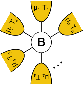
Figure 1: Sketch of the multi-terminal model for thermoelectric transport

We consider the set-up schematically shown in figure 1. A central scattering region equipped with a constant magnetic field $\mathbf{B}$ is connected to $n$ independent electronic reservoirs (terminals) of respective temperature $T_{1},\dots,T_{n}$ and chemical potential $\mu_{1},\dots\mu_{n}$. We assume non interacting electrons, which are transferred coherently between the terminals without any inelastic scattering. In order to describe the resulting transport process within the framework of linear irreversible thermodynamics, we fix the reference temperature $T\equiv T_{1}$ and chemical potential $\mu\equiv\mu_{1}$, and define the affinities

$$\mathcal{F}^{\rho}_{\alpha}\equiv\frac{\mu_{\alpha}-\mu}{T}\equiv\frac{\Delta\mu_{\alpha}}{T}\qquad{{\rm and}}\qquad\mathcal{F}^{q}_{\alpha}\equiv\frac{T_{\alpha}-T}{T^{2}}\equiv\frac{\Delta T_{\alpha}}{T^{2}}$$ (1)

$$\left(\alpha=2,\dots n\right).$$

By $J^{\rho}_{\alpha}$ and $J^{q}_{\alpha}$ we denote the charge and the heat current flowing out of the reservoir $\alpha$, respectively. Within the linear response regime, which is valid as long as the temperature and chemical potential differences $\Delta T_{\alpha}$ and $\Delta\mu_{\alpha}$ are small compared to the respective reference values, the currents and affinities are connected via the phenomenological equations [18]

$$\mathbf{J}=\mathbb{L}(\mathbf{B})\boldsymbol{\mathcal{F}}.$$ (2)

Here, we introduced the current vector

$$\mathbf{J}\equiv\left(\!\begin{array}[]{c}\mathbf{J}_{2}\\ \vdots\\ \mathbf{J}_{n}\end{array}\!\right)\qquad{{\rm and}}\;{{\rm the}}\;{{\rm affinity}}\;{{\rm vector}}\qquad\boldsymbol{\mathcal{F}}=\left(\!\begin{array}[]{c}\boldsymbol{\mathcal{F}}_{2}\\ \vdots\\ \boldsymbol{\mathcal{F}}_{n}\end{array}\!\right)$$ (3)

with the respective subunits

$$\mathbf{J}_{\alpha}\equiv\left(\!\begin{array}[]{c}J^{\rho}_{\alpha}\\ J^{q}_{\alpha}\end{array}\!\right)\qquad{{\rm and}}\quad\boldsymbol{\mathcal{F}}_{\alpha}\equiv\left(\!\begin{array}[]{c}\mathcal{F}_{\alpha}^{\rho}\\ \mathcal{F}_{\alpha}^{q}\end{array}\!\right).$$ (4)

Analogously, we divide the matrix of kinetic coefficients

$$\mathbb{L}(\mathbf{B})\equiv\left(\!\begin{array}[]{ccc}\mathbb{L}_{22}(\mathbf{B})&\cdots&\mathbb{L}_{2n}(\mathbf{B})\\ \vdots&\ddots&\vdots\\ \mathbb{L}_{n2}(\mathbf{B})&\cdots&\mathbb{L}_{nn}(\mathbf{B})\end{array}\!\right)\in\mathbb{R}^{2(n-1)\times 2(n-1)}$$ (5)

into the $2\times 2$ blocks $\mathbb{L}_{\alpha\beta}\in\mathbb{R}^{2\times 2}$ ($\alpha,\beta=2,\dots,n$), which can be calculated explicitly. By making use of the multi-terminal Landauer formula [11, 12], we get the expression

$$\mathbb{L}_{\alpha\beta}(\mathbf{B})=\frac{Te^{2}}{h}\int_{-\infty}^{\infty}dE\;F(E)\left(\!\begin{array}[]{cc}1&\frac{E-\mu}{e}\\ \frac{E-\mu}{e}&\left(\frac{E-\mu}{e}\right)^{2}\end{array}\!\right)\left(\delta_{\alpha\beta}-T_{\alpha\beta}(E,\mathbf{B})\right),$$ (6)

where $h$ denotes Planck’s constant, $e$ the electronic unit charge,

$$F(E)\equiv\left[4k_{B}T\cosh^{2}\left(\frac{E-\mu}{2k_{B}T}\right)\right]^{-1}$$ (7)

the negative derivative of the Fermi function and $k_{B}$ Boltzmann’s constant.

The expression (6) shows that the transport properties of the model are completely determined by the transition probabilities $T_{\alpha\beta}(E,\mathbf{B})$, which obey two important relations. First, current conservation requires the sum rule

$$\sum_{\alpha=1}^{n}T_{\alpha\beta}(E,\mathbf{B})=\sum_{\beta=1}^{n}T_{\alpha\beta}(E,\mathbf{B})=1,$$ (8)

i.e., the transition matrix

$$\mathbb{T}(E,\mathbf{B})\equiv\left(\!\begin{array}[]{ccc}T_{11}(E,\mathbf{B})&\cdots&T_{1n}(E,\mathbf{B})\\ \vdots&\ddots&\vdots\\ T_{n1}(E,\mathbf{B})&\cdots&T_{nn}(E,\mathbf{B})\end{array}\!\right)\in\mathbb{R}^{n\times n}$$ (9)

is doubly stochastic for any $E\in\mathbb{R}$ and $\mathbf{B}\in\mathbb{R}^{3}$. Second, due to time reversal symmetry, the $T_{\alpha\beta}(E,\mathbf{B})$ have to posses the symmetry

$$T_{\alpha\beta}(E,\mathbf{B})=T_{\beta\alpha}(E,-\mathbf{B}).$$ (10)

Notably, for a fixed magnetic field $\mathbf{B}$, the transition matrix $\mathbb{T}(E,\mathbf{B})$ does not necessarily have to be symmetric. This observation will be crucial for the subsequent considerations.

For later purpose, we note that, by combining (5) and (6), $\mathbb{L}(\mathbf{B})$ can be expressed as an integral over tensor products given by

$$\mathbb{L}(\mathbf{B})=\frac{Te^{2}}{h}\int_{-\infty}^{\infty}dE\;F(E)\left(\mathbbm{1}-\bar{\mathbb{T}}(E,\mathbf{B})\right)\otimes\left(\!\begin{array}[]{cc}1&\frac{E-\mu}{e}\\ \frac{E-\mu}{e}&\left(\frac{E-\mu}{e}\right)^{2}\end{array}\!\right).$$ (11)

Here, $\mathbbm{1}$ denotes the identity matrix and $\bar{\mathbb{T}}(E,\mathbf{B})$ arises from $\mathbb{T}(E,\mathbf{B})$ by deleting the first row and column. Consequently, the matrix $\bar{\mathbb{T}}(E,\mathbf{B})$ must be doubly substochastic, which means that all entries of $\bar{\mathbb{T}}(E,\mathbf{B})$ are non-negative and any row and column sums up to a value not greater than $1$.

3 Bounds on the Kinetic Coefficients

3.1 Phenomenological Constraints

The phenomenological framework of linear irreversible thermodynamics provides two fundamental constraints on the matrix of kinetic coefficients $\mathbb{L}(\mathbf{B})$. First, since the entropy production accompanying the transport process descibed by (2) reads [18]

$$\dot{S}=\boldsymbol{\mathcal{F}}^{t}\mathbf{J}=\boldsymbol{\mathcal{F}}^{t}\mathbb{L}(\mathbf{B})\boldsymbol{\mathcal{F}},$$ (12)

the second law requires $\mathbb{L}(\mathbf{B})$ to be positive semi-definite. Second, Onsager’s reciprocal relations impose the symmetry

$$\mathbb{L}^{t}(\mathbf{B})=\mathbb{L}(-\mathbf{B}).$$ (13)

Apart from these constraints, no further general relations restricting the elements of $\mathbb{L}(\mathbf{B})$ at fixed magnetic field $\mathbf{B}$ are known. We will now demonstrate that such a lack of constraints leads to profound consequences for the thermodynamical properties of this model. To this end, we split the current vector $\mathbf{J}$ into an irreversible and a reversible part given by

$$\mathbf{J}^{{{\rm irr}}}\equiv\frac{\mathbb{L}(\mathbf{B})+\mathbb{L}^{t}(\mathbf{B})}{2}\boldsymbol{\mathcal{F}}\qquad{{\rm and}}\qquad\mathbf{J}^{{{\rm rev}}}\equiv\frac{\mathbb{L}(\mathbf{B})-\mathbb{L}^{t}(\mathbf{B})}{2}\boldsymbol{\mathcal{F}}$$ (14)

respectively. The reversible part vanishes for $\mathbf{B}=\boldsymbol{0}$ by virtue of the reciprocal relations (13). However, in situations with $\mathbf{B}\neq\boldsymbol{0}$ it can become arbitrarily large without contributing to the entropy production (12). In principle, it would be even possible to have $\dot{S}=0$ and $\mathbf{J}^{{{\rm rev}}}\neq\boldsymbol{0}$ simultaneously, i.e., completely reversible transport, suggesting inter alia the opportunity for a thermoelectric heat engine operating at Carnot efficiency with finite power output [9]. This observation raises the question, whether there might be stronger relations between the kinetic coefficients going beyond the well known reciprocal relations (13). In the next section, starting from the microscopic representation (6), we derive bounds on the kinetic coefficients, which prevent this option of Carnot efficiency with finite power.

3.2 Bounds following from Current Conservation

These bounds can be derived by first quantifying the asymmetry of the Onsager matrix $\mathbb{L}(\mathbf{B})$. For an arbitrary positive semi-definite matrix $\mathbb{A}\in\mathbb{R}^{m\times m}$ we define an asymmetry index by

$$\mathcal{S}(\mathbb{A})\equiv\min\left\{\left.s\in\mathbb{R}\right|\forall\mathbf{z}\in\mathbb{C}^{m}\;\;\;\mathbf{z}^{\dagger}\left(s\left(\mathbb{A}+\mathbb{A}^{t}\right)+i\left(\mathbb{A}-\mathbb{A}^{t}\right)\right)\mathbf{z}\geq 0\right\}.$$ (15)

Some of the basic properties of this asymmetry index are outlined in A. We note that a quite similar quantity was introduced by Crouzeix and Gutan [19] in another context.

We will now proceed in two steps. First, we show that the asymmetry index of the matrix of kinetic coefficients $\mathbb{L}(\mathbf{B})$ and all its principal submatrices is bounded from above for any finite number of terminals $n$. Second, we will derive therefrom a set of new bounds on the elements of $\mathbb{L}(\mathbf{B})$, which go beyond the second law. We note that from now on we notationally suppress the dependence of any quantity on the magnetic field in order to keep the notation slim.

For the first step, we define the quadratic form

$$Q(\mathbf{z},s)\equiv\mathbf{z}^{\dagger}\left(s\left(\mathbb{L}_{A}+\mathbb{L}^{t}_{A}\right)+i\left(\mathbb{L}_{A}-\mathbb{L}^{t}_{A}\right)\right)\mathbf{z}$$ (16)

for any $\mathbf{z}\in\mathbb{C}^{2m}$ and any $s\in\mathbb{R}$. Here, $A\subset\left\{2,\dots,n\right\}$ denotes a set of $m\leq n-1$ integers. The matrix $\mathbb{L}_{A}$ arises from $\mathbb{L}$ by taking all blocks $\mathbb{L}_{\alpha\beta}$ with column and row index in $A$, i.e., $\mathbb{L}_{A}$ is a principal submatrix of $\mathbb{L}$, which preserves the $2\times 2$ block structure shown in (5). Comparing (16) with the definition (15) reveals that the minimum $s$ for which $Q(\mathbf{z},s)$ is positive semi-definite equals the asymmetry index of $\mathbb{L}_{A}$. Next, by recalling (11) we rewrite the matrix $\mathbb{L}_{A}$ in the rather compact form

$$\mathbb{L}_{A}=\frac{Te^{2}}{h}\int_{-\infty}^{\infty}dE\;F(E)\left(\mathbbm{1}-\bar{\mathbb{T}}_{A}(E)\right)\otimes\left(\!\begin{array}[]{cc}1&\frac{E-\mu}{e}\\ \frac{E-\mu}{e}&\left(\frac{E-\mu}{e}\right)^{2}\end{array}\!\right),$$ (17)

where $\bar{\mathbb{T}}_{A}(E)\in\mathbb{R}^{m\times m}$ is obtained from $\bar{\mathbb{T}}(E)$ by taking the rows and columns indexed by the set $A$. Decomposing the vector $\mathbf{z}$ as

$$\mathbf{z}\equiv\mathbf{z}_{1}\otimes\left(\!\begin{array}[]{c}1\\ 0\end{array}\!\right)+\mathbf{z}_{2}\otimes\left(\!\begin{array}[]{c}0\\ 1\end{array}\!\right)\qquad{{\rm with}}\qquad\mathbf{z}_{1},\mathbf{z}_{2}\in\mathbb{C}^{m}$$ (18)

and inserting (17) and (18) into (16) yields

$$Q(\mathbf{z},s)=\frac{Te^{2}}{h}\int_{-\infty}^{\infty}dE\;F(E)\mathbf{y}^{\dagger}(E)\mathbb{K}(E,s)\mathbf{y}(E).$$ (19)

Here we introduced the vector

$$\mathbf{y}(E)\equiv\mathbf{z}_{1}+\frac{E-\mu}{e}\mathbf{z}_{2}$$ (20)

and the Hermitian matrix

$$\mathbb{K}_{A}(E,s)\equiv s\left(2\cdot\mathbbm{1}-\bar{\mathbb{T}}_{A}(E)-\bar{\mathbb{T}}^{t}_{A}(E)\right)-i\left(\bar{\mathbb{T}}_{A}(E)-\bar{\mathbb{T}}^{t}_{A}(E)\right)\in\mathbb{C}^{m\times m},$$

which is positive semi-definite for any

$$s\geq\mathcal{S}\left(\mathbbm{1}-\bar{\mathbb{T}}_{A}(E)\right).$$ (22)

However, since $\bar{\mathbb{T}}(E)$ is doubly stochastic for any $E$, the matrix $\bar{\mathbb{T}}_{A}(E)$ must have the same property and it follows from Corollary 2 proven in B

$$\mathcal{S}\left(\mathbbm{1}-\bar{\mathbb{T}}_{A}(E)\right)\leq\cot\left(\frac{\pi}{m+1}\right).$$ (23)

Hence, independently of $E$, $\mathbb{K}_{A}(E,s)$ is positive semi-definite for any

$$s\geq\cot\left(\frac{\pi}{m+1}\right).$$ (24)

Finally, we can infer from (19) that $Q(\mathbf{z},s)$ is positive semi-definite for any $s$, which obeys (24). Consequently, with (16), we have the desired bound on the asymmetry index of $\mathbb{L}_{A}$ as

$$\mathcal{S}\left(\mathbb{L}_{A}\right)\leq\cot\left(\frac{\pi}{m+1}\right).$$ (25)

This bound, which ultimately follows from current conservation, constitutes our first main result.

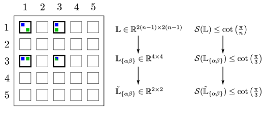
Figure 2: Schematic illustration of the reduction from $\mathbb{L}$ to $\tilde{\mathbb{L}}_{\alpha\beta}$. The big square represents $\mathbb{L}$ for the case $n=6$, the smaller ones correspond to the $2\times 2$ blocks introduced in (5). By taking the bold framed squares, the $4\times 4$ matrix $\mathbb{L}_{\{\alpha\beta\}}$ is obtained for the case $\alpha=1$ and $\beta=3$. The filled squares represent the elements of the $2\times 2$ matrix $\tilde{\mathbb{L}}_{\{\alpha\beta\}}$ introduced in (28) for $(i,j)=(1,1)$ (blue) and $(i,j)=(2,1)$ (green).

We will now demonstrate that (25) puts indeed strong bounds on the kinetic coefficients. To this end, we extract a $2\times 2$ principal submatrix from $\mathbb{L}$ by a two-step procedure, which is schematically summarized in figure 2. In the first step, we consider the $4\times 4$ principal submatrix of $\mathbb{L}$ given by

$${\mathbb{L}}_{\{\alpha,\beta\}}\equiv\left(\!\begin{array}[]{cc}\mathbb{L}_{\alpha\alpha}&\mathbb{L}_{\alpha\beta}\\ \mathbb{L}_{\beta\alpha}&\mathbb{L}_{\beta\beta}\end{array}\!\right),$$ (26)

which arises from $\mathbb{L}$ by taking only the blocks with row and column index equal to $\alpha$ or $\beta$. From (25) we immediately get with $m=2$

$$\mathcal{S}\left(\mathbb{L}_{\{\alpha,\beta\}}\right)\leq\cot\left(\frac{\pi}{3}\right)=\frac{1}{\sqrt{3}}.$$ (27)

Next, from (26), we take a $2\times 2$ principal submatrix

$$\tilde{\mathbb{L}}_{\{\alpha,\beta\}}\equiv\left(\!\begin{array}[]{cc}\left(\mathbb{L}_{\alpha\alpha}\right)_{ii}&\left(\mathbb{L}_{\alpha\beta}\right)_{ij}\\ \left(\mathbb{L}_{\beta\alpha}\right)_{ji}&\left(\mathbb{L}_{\beta\beta}\right)_{jj}\end{array}\!\right)\equiv\left(\!\begin{array}[]{cc}L_{11}&L_{12}\\ L_{21}&L_{22}\end{array}\!\right),$$ (28)

where $\left(\mathbb{L}_{\alpha\beta}\right)_{ij}$ with $i,j=1,2$ denotes the $(i,j)$-entry of the block matrix $\mathbb{L}_{\alpha\beta}$. By virtue of Proposition 3 proven in B, the inequality (27) implies

$$\mathcal{S}\left(\tilde{\mathbb{L}}_{\{\alpha,\beta\}}\right)\leq\frac{1}{\sqrt{3}},$$ (29)

which is equivalent to requiring the Hermitian matrix

$$\tilde{\mathbb{K}}_{\{\alpha,\beta\}}\equiv\frac{1}{\sqrt{3}}\left(\tilde{\mathbb{L}}_{\{\alpha,\beta\}}+\tilde{\mathbb{L}}_{\{\alpha,\beta\}}^{t}\right)+i\left(\tilde{\mathbb{L}}_{\{\alpha,\beta\}}-\tilde{\mathbb{L}}_{\{\alpha,\beta\}}^{t}\right)=\left(\begin{array}[]{cc}K_{11}&K_{12}\\ K_{12}^{\ast}&K_{22}\end{array}\right)$$ (30)

to be positive semi-definite. Since the diagonal entries of $\tilde{\mathbb{K}}_{\{\alpha,\beta\}}$ are obviously non-negative, this condition reduces to ${{\rm Det}}\tilde{\mathbb{K}}_{\{\alpha,\beta\}}=K_{11}K_{22}-\left|K_{12}\right|^{2}\geq 0.$ Finally, expressing the $K_{ij}$ again in terms of the $L_{ij}$ yields the new constraint

$$4L_{11}L_{22}-(L_{12}+L_{21})^{2}\geq 3\left(L_{12}-L_{21}\right)^{2}.$$ (31)

This bound that holds for the elements of any $2\times 2$ principal submatrix of the full matrix of kinetic coefficients $\mathbb{L}$, irrespective of the number $n$ of terminals is our second main result. Compared to relation (31), the second law only requires $\tilde{\mathbb{L}}_{\{\alpha,\beta\}}$ to be positive semi-definite, which is equivalent to $L_{11},\;L_{22}\geq 0$ and the weaker constraint

$$4L_{11}L_{22}-\left(L_{12}+L_{21}\right)^{2}\geq 0.$$ (32)

Note that the reciprocal relations (13) do not lead to any further relations between the kinetic coefficients contained in $\tilde{\mathbb{L}}_{\{\alpha,\beta\}}$ for a fixed magnetic field $\mathbf{B}$.

At this point, we emphasize that the procedure shown here for $2\times 2$ principal submatrices of $\mathbb{L}$ could be easily extended to larger principal submatrices. The result would be a whole hierachy of constraints involving more and more kinetic coefficients. However, (31) is the strongest bound following from (25), which can expressed in terms of only four of these coefficients.

4 Bounds on Efficiencies

In this section, we explore the consequences of the bound (25) on the performance of various thermoelectric devices.

4.1 Heat engine

A thermoelectric heat engine uses heat from a hot reservoir as input and generates power output by driving a particle current against an external field or a gradient of chemical potential [5]. Such an engine can be realized within the multi-terminal model by considering the terminals $3,\dots,n$ as pure probe terminals, which mimic inelastic scattering events while not contributing to the actual transport process. This constraint reads

$$\left(\!\begin{array}[]{c}0\\ \vdots\\ 0\end{array}\!\right)=\left(\!\begin{array}[]{c}\mathbf{J}_{3}\\ \vdots\\ \mathbf{J}_{n}\end{array}\!\right)=\left(\!\begin{array}[]{ccc}\mathbb{L}_{32}&\cdots&\mathbb{L}_{3n}\\ \vdots&\ddots&\vdots\\ \mathbb{L}_{n2}&\cdots&\mathbb{L}_{nn}\end{array}\!\right)\left(\!\begin{array}[]{c}\boldsymbol{\mathcal{F}}_{2}\\ \vdots\\ \boldsymbol{\mathcal{F}}_{n}\end{array}\!\right).$$ (33)

By assuming the matrix

$$\mathbb{L}_{\{3,\dots,n\}}\equiv\left(\!\begin{array}[]{ccc}\mathbb{L}_{33}&\cdots&\mathbb{L}_{3n}\\ \vdots&\ddots&\vdots\\ \mathbb{L}_{n3}&\cdots&\mathbb{L}_{nn}\end{array}\!\right)$$ (34)

to be invertible, we can solve the self-consistency relations (33) for $\boldsymbol{\mathcal{F}}_{3},\dots,\boldsymbol{\mathcal{F}}_{n}$ obtaining

$$\left(\!\begin{array}[]{c}\boldsymbol{\mathcal{F}}_{3}\\ \vdots\\ \boldsymbol{\mathcal{F}}_{n}\end{array}\!\right)=-\left(\mathbb{L}_{\{3,\dots,n\}}\right)^{-1}\left(\!\begin{array}[]{c}\mathbb{L}_{32}\\ \vdots\\ \mathbb{L}_{n3}\end{array}\!\right)\boldsymbol{\mathcal{F}}_{2}.$$ (35)

After inserting this solution into (2) and identifying the heat current $J_{q}\equiv J_{2}^{q}$ leaving the hot reservoir and the particle current $J_{\rho}\equiv J_{2}^{\rho}$, we end up with the reduced system

$$\left(\!\begin{array}[]{c}J_{\rho}\\ J_{q}\end{array}\!\right)=\mathbb{L}^{{{\rm HE}}}\left(\!\begin{array}[]{c}\mathcal{F}_{\rho}\\ \mathcal{F}_{q}\end{array}\!\right),$$ (36)

of phenomenological equations. Here, the effective matrix of kinetic coefficients is given by

$$\mathbb{L}^{{{\rm HE}}}\equiv\mathbb{L}_{22}-\left(\mathbb{L}_{23},\cdots,\mathbb{L}_{2n}\right)\left(\mathbb{L}_{\{3,\dots,n\}}\right)^{-1}\left(\!\begin{array}[]{c}\mathbb{L}_{32}\\ \vdots\\ \mathbb{L}_{n3}\end{array}\!\right)\equiv\left(\!\begin{array}[]{cc}L_{\rho\rho}&L_{\rho q}\\ L_{q\rho}&L_{qq}\end{array}\!\right)$$ (37)

and the affinities $\mathcal{F}_{\rho}\equiv\mathcal{F}_{2}^{\rho}=\Delta\mu_{2}/T<0$ and $\mathcal{F}_{q}\equiv\mathcal{F}_{2}^{q}=\Delta T_{2}/T^{2}>0$ have to be chosen such that $J_{\rho},J_{q}\geq 0$ for the model to work as a proper heat engine.

$\mathbb{L}^{{{\rm HE}}}$ is not a principal submatrix of the full Onsager matrix $\mathbb{L}$ and therefore the bound (25) does not apply directly. However, $\mathbb{L}^{{{\rm HE}}}$ can be written as the Schur complement $\mathbb{L}/\mathbb{L}_{\{3,\dots,n\}}$ (see C for the definition), the asymmetry index of which is dominated by the asymmetry index of $\mathbb{L}$ as proven in Proposition 4 of C. Consequently, we have

$$\mathcal{S}\left(\mathbb{L}^{{{\rm HE}}}\right)=\mathcal{S}\left(\mathbb{L}/\mathbb{L}_{\{3,\dots,n\}}\right)\leq\mathcal{S}\left(\mathbb{L}\right)\leq\cot\left(\frac{\pi}{n}\right).$$ (38)

or, equivalently,

$$4L_{\rho\rho}L_{qq}-\left(L_{\rho q}+L_{q\rho}\right)^{2}\geq\tan^{2}\left(\frac{\pi}{n}\right)\left(L_{\rho q}-L_{q\rho}\right)^{2}.$$ (39)

This constraint shows that whenever $L_{\rho q}\neq L_{q\rho}$, the entropy production (12) must be strictly larger than zero, thus ruling out the option of dissipationless transport generated solely by reversible currents for any model with a finite number $n$ of terminals. For any $n>3$ this constraint is weaker than (31). The reason is that the Onsager coefficients in (39) are not elements of the full matrix (5) but rather involve the inversion of $\mathbb{L}_{\{3,\dots,n\}}$ defined in (34). Still, this constraint is stronger than the bare second law, which requires only

$$4L_{\rho\rho}L_{qq}-\left(L_{\rho q}+L_{q\rho}\right)^{2}\geq 0,$$ (40)

irrespective of whether or not $\mathbb{L}^{{{\rm HE}}}$ is symmetric.

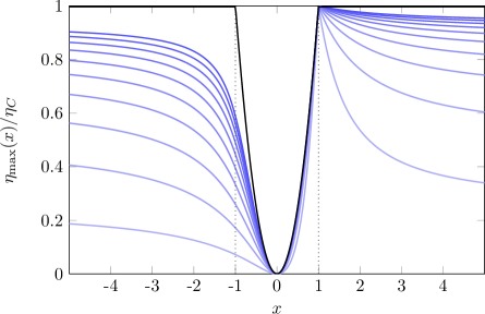
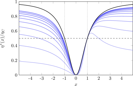
Figure 3: Bounds on the efficiency of the multi-terminal model as a thermoelectric heat engine as functions of the asymmetry parameter $x$ and in units of $\eta_{C}$. The upper panel shows $\eta_{{{\rm max}}}(x)$ (see (46)), the lower one $\eta^{\ast}(x)$ (see (49)). In both panels, the blue lines, from bottom to top, belong to models with $n=3,\dots,12$ terminals and the solid, black line corresponds to the bound following from the bare second law as obtained by Benenti et al[9]. The dashed line in the lower panel marks the Curzon-Ahlborn limit $\eta_{CA}=\eta_{C}/2$.

The constraint (39) implies a constraint on the efficiency $\eta$ of such a particle-exchange heat engine [5], which is defined as

$$\eta\equiv-\frac{\Delta\mu_{2}J_{\rho}}{J_{q}}\leq\eta_{C}.$$ (41)

Like for any heat engine, this efficiency is subject to the Carnot-bound $\eta_{C}\equiv 1-T/T_{2}$, which, in the linear response regime, is given by $\eta_{C}\approx\Delta T_{2}/T=T\mathcal{F}_{q}$. Following Benenti et al[9], we now introduce the dimensionless parameters

$$y\equiv\frac{L_{\rho q}L_{q\rho}}{L_{\rho\rho}L_{qq}-L_{\rho q}L_{q\rho}}\qquad{{{\rm and}}}\qquad x\equiv\frac{L_{\rho q}}{L_{q\rho}},$$ (42)

which allow us to write the maximum efficiency of the engine $\eta_{{{\rm max}}}$ (under the condition $J_{q}>0$) in the instructive form [9]

$$\eta_{{{\rm max}}}(x,y)=\eta_{C}x\frac{\sqrt{y+1}-1}{\sqrt{y+1}+1}.$$ (43)

Restating the new bound (39) in terms of $x$ and $y$ yields

$$\begin{array}[]{lll}h_{n}(x)\leq y\leq 0&\quad{{\rm if}}&x<0,\\ 0\leq y\leq h_{n}(x)&\quad{{\rm if}}&x>0\end{array}$$ (44)

with

$$h_{n}(x)\equiv\frac{4x}{(x-1)^{2}}\cos^{2}\left(\frac{\pi}{n}\right).$$ (45)

Consequently, maximizing (43) with respect to $y$ yields the optimal $y^{\ast}(x)=h_{n}(x)$ and the maximum efficiency

$$\eta_{{{\rm max}}}(x)\equiv\eta_{{{\rm max}}}(x,y^{\ast}(x))=\eta_{C}x\frac{\sqrt{4x\cos^{2}(\pi/n)+(x-1)^{2}}-|x-1|}{\sqrt{4x\cos^{2}(\pi/n)+(x-1)^{2}}+|x-1|}.$$ (46)

This bound is plotted in figure 3 as a function of $x$ for an increasing number $n$ of terminals. For $n=3$, we recover the result obtained in our preceding work on the three terminal model [16]. In the limit $n\rightarrow\infty$, $\eta_{{{\rm max}}}(x)$ converges to the bound derived by Benenti et al[9] within a general analysis relying only on the second law. However, for any finite $n$, $\eta_{{{\rm max}}}(x)$ is constrained to be strictly smaller than $\eta_{C}$, as soon as $x$ deviates from $1$. Thus, from the perspective of maximum efficiency, breaking the time reversal symmetry is not beneficial.

As a second important benchmark for the performance of a heat engine, we consider its efficiency at maximum power $\eta^{\ast}$ [20, 21, 22] obtained by maximizing the power output

$$P_{{{\rm out}}}\equiv-\Delta\mu_{2}J_{\rho}=-T\mathcal{F}_{\rho}\left(L_{\rho\rho}\mathcal{F}_{\rho}+L_{\rho q}\mathcal{F}_{q}\right)$$ (47)

with respect to $\mathcal{F}_{\rho}$ for fixed $\mathcal{F}_{q}$. In terms of the dimensionless parameters (42), it reads [9]

$$\eta^{\ast}(x,y)=\eta_{C}\frac{xy}{4+2y}$$ (48)

and attains its maximum

$$\eta^{\ast}(x)\equiv\eta^{\ast}(x,y^{\ast}(x))=\eta_{C}\frac{x^{2}\cos^{2}(\pi/n)}{(x-1)^{2}+2x\cos^{2}(\pi/n)}$$ (49)

at $y^{\ast}(x)=h_{n}(x)$. In the lower panel of figure 3, $\eta^{\ast}(x)$ is plotted as a function of the asymmetry parameter $x$. For $x=1$, this bound acquires the Curzon-Ahlborn value $\eta_{CA}\equiv\eta_{C}/2$. For $x\neq 1$, however it can become significantly higher even for a small number $n$ of terminals. Specifically, we observe that $\eta^{\ast}(x)$ exceeds $\eta_{CA}$ for any $n\geq 3$ in a certain range of $x$ values. For $n\geq 4$, this range includes all $x>1$. Furthermore, $\eta^{\ast}(x)$ attains its global maximum

$$\hat{\eta}^{\ast\ast}\equiv\frac{\eta_{C}}{1+\sin^{2}\left(\frac{\pi}{n}\right)}$$ (50)

at the finite value $x=1/\sin^{2}\left(\frac{\pi}{n}\right)$. Remarkably, both $\eta_{{{\rm max}}}(x)$ and $\eta^{\ast}(x)$ approach the same asymptotic value $\eta^{\infty}\equiv\eta_{C}\cos^{2}\left(\frac{\pi}{n}\right)$ for $x\rightarrow\pm\infty$.

4.2 Refrigerator

In the preceding section, we discussed the performance of the multi-terminal model if it is operated as a heat engine. Quite naturally, we can change the mode of operation of this engine such that it functions as a refrigerator. The resulting device consumes electrical power from which it generates a heat current from the cold to the hot reservoir. Thus, compared to the heat engine, input and output are interchanged and the affinities $\mathcal{F}_{\rho}<0$ and $\mathcal{F}_{q}>0$ have to be chosen such that both currents $J_{\rho}$ and $J_{q}$ are negative.

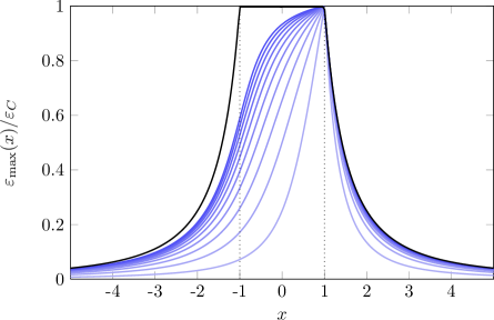
Figure 4: Maximum coefficient of performance $\varepsilon_{{{\rm max}}}(x)$ (see (53)) of a thermoelectric refrigerator as a function of the asymmetry parameter $x$. The blue lines from bottom to top represent models with $n=3,\dots,12$ terminals. The black curve shows the bound required by the bare second law, which is asymptotically reached in the limit $n\rightarrow\infty$.

Analogously to the case of the heat engine, we will now show that the bound (39) on the kinetic coefficients constrains the performance of the thermoelectric refrigerator described above. To this end, we will use the coefficient of performance [18]

$$\varepsilon\equiv-\frac{J_{q}}{\Delta\mu_{2}J_{\rho}}.$$ (51)

as a benchmark parameter. Its upper bound following from the second law is given by $\varepsilon_{C}\equiv T/\Delta T_{2}=1/(T\mathcal{F}_{q})$, which is the efficiency of the ideal refrigerator. In this sense, $\varepsilon_{C}$ is the analogue to the Carnot efficiency.

Taking the maximum of $\varepsilon$ over $\mathcal{F}_{\rho}$ (under the condition $J_{\rho}<0$) while keeping $\mathcal{F}_{q}$ fixed, yields the maximum coefficient of performance [9]

$$\varepsilon_{{{\rm max}}}(x,y)=\frac{\varepsilon_{C}}{x}\frac{\sqrt{y+1}-1}{\sqrt{y+1}+1}.$$ (52)

Here, we used again the dimensionless parameters defined in (42). Since $y$ is subject to the constraint (44), $\varepsilon_{{{\rm max}}}(x,y)$ attains its maximum

$$\varepsilon_{{{\rm max}}}(x)\equiv\varepsilon_{{{\rm max}}}(x,y^{\ast}(x))=\frac{\varepsilon_{C}}{x}\frac{\sqrt{4x\cos^{2}(\pi/n)+(x-1)^{2}}-|x-1|}{\sqrt{4x\cos^{2}(\pi/n)+(x-1)^{2}}+|x-1|}$$ (53)

with respect to $y$ at $y^{\ast}(x)=h_{n}(x)$, where $h_{n}(x)$ was introduced in (45). Figure 4 shows $\eta_{{{\rm max}}}(x)$ for models with an increasing number of probe terminals $n$. For any finite $n$, $\varepsilon_{C}$ can only be reached for the symmetric value $x=1$. The black line follows solely from the second law (40) and would in principle allow to reach $\varepsilon_{C}$ with finite current for $x$ between $-1$ and $1$. However, like for the heat engine, our analysis reveals that such a high performance refrigerator would need to be equipped with an infinite number of terminals.

4.3 Isothermal Engine

By an isothermal, thermoelectric engine, we understand in this context a device in which one particle current driven by a (negative) gradient in chemical potential drives another one uphill a chemical potential gradient at constant temperature $T$. In order to implement such a machine within the multi-terminal framework, we put $\mathcal{F}_{2}^{q}=\cdots=\mathcal{F}_{n}^{q}=0$. The remaining affinities $\mathcal{F}_{2}^{\rho},\dots,\mathcal{F}_{n}^{\rho}$ are connected to the particle currents via a reduced set of phenomenological equations given by

$$\left(\!\begin{array}[]{c}J^{\rho}_{2}\\ \vdots\\ J^{\rho}_{n}\end{array}\!\right)=\left(\!\begin{array}[]{ccc}(\mathbb{L}_{22})_{11}&\cdots&(\mathbb{L}_{2n})_{11}\\ \vdots&\ddots&\vdots\\ (\mathbb{L}_{n2})_{11}&\cdots&(\mathbb{L}_{nn})_{11}\end{array}\!\right)\left(\!\begin{array}[]{c}\mathcal{F}^{\rho}_{2}\\ \vdots\\ \mathcal{F}^{\rho}_{n}\end{array}\!\right),$$ (54)

where $(\mathbb{L}_{\alpha\beta})_{11}$ denotes the (11)-entry of the block matrix $\mathbb{L}_{\alpha\beta}$ defined in (6). We note that the heat currents $J^{q}_{2},\dots,J^{q}_{n}$ do not necessarily have to vanish. However, since they do not contribute to the entropy production (12), they are irrelevant in the present analysis. Similar to the treatment of the heat engine, we put $J^{\rho}_{4}=\cdots=J^{\rho}_{n}=0$, thus considering the terminals $4,\dots,n$ as pure probe terminals simulating inelastic scattering events. Consequently, (54) can be reduced further to the generic form

$$\left(\!\begin{array}[]{c}J_{2}^{\rho}\\ J_{3}^{\rho}\end{array}\!\right)=\mathbb{L}^{{{\rm IE}}}\left(\!\begin{array}[]{c}\mathcal{F}_{2}^{\rho}\\ \mathcal{F}_{3}^{\rho}\end{array}\!\right).$$ (55)

Here, we have introduced the matrix

$$\mathbb{L}^{{{\rm IE}}} \equiv\left.\left(\!\begin{array}[]{ccc}(\mathbb{L}_{22})_{11}&\cdots&(\mathbb{L}_{2n})_{11}\\ \vdots&\ddots&\vdots\\ (\mathbb{L}_{n2})_{11}&\cdots&(\mathbb{L}_{nn})_{11}\end{array}\!\right)\right/\left(\!\begin{array}[]{ccc}(\mathbb{L}_{44})_{11}&\cdots&(\mathbb{L}_{4n})_{11}\\ \vdots&\ddots&\vdots\\ (\mathbb{L}_{n4})_{11}&\cdots&(\mathbb{L}_{nn})_{11}\end{array}\!\right)$$ (62)

$$\equiv\left(\!\begin{array}[]{cc}L_{22}&L_{23}\\ L_{32}&L_{33}\end{array}\!\right)$$ (65)

again using the Schur complement defined in C. The affinities $\mathcal{F}^{\rho}_{2},\mathcal{F}^{\rho}_{3}>0$ have to be chosen such that $J^{\rho}_{2}$ is negative and $J^{\rho}_{3}$ is positive to ensure that the device pumps particles into the reservoir $2$ against the gradient in chemical potential $\Delta\mu_{2}$.

We will now derive a bound on the elements of $\mathbb{L}^{{{\rm IE}}}$. By employing expression (11), we can write

$$\left(\!\begin{array}[]{ccc}(\mathbb{L}_{22})_{11}&\cdots&(\mathbb{L}_{2n})_{11}\\ \vdots&\ddots&\vdots\\ (\mathbb{L}_{n2})_{11}&\cdots&(\mathbb{L}_{nn})_{11}\end{array}\!\right) =\frac{Te^{2}}{h}\int_{-\infty}^{\infty}dE\;F(E)\left(\mathbbm{1}-\bar{\mathbb{T}}(E)\right)$$ (69)

$$\equiv\mathcal{N}\left(\mathbbm{1}-\langle\bar{\mathbb{T}}\rangle\right)$$ (70)

with

$$\mathcal{N}\equiv\frac{Te^{2}}{h}\int_{-\infty}^{\infty}dE\;F(E)=\frac{Te^{2}}{h}$$ (71)

and

$$\langle\bar{\mathbb{T}}\rangle\equiv\int_{-\infty}^{\infty}dE\;F(E)\bar{\mathbb{T}}(E).$$ (72)

Since $\bar{\mathbb{T}}(E)$ is doubly substochastic for any $E$, the matrix $\langle\bar{\mathbb{T}}\rangle$ is also doubly substochastic. Therefore, by applying Corollary 3 of C, we find

$$\mathcal{S}\left(\mathbb{L}^{{{\rm IE}}}\right)=\mathcal{S}\left(\frac{\mathbb{L}^{{{\rm IE}}}}{\mathcal{N}}\right) =\mathcal{S}\left(\left.\left(\mathbbm{1}-\langle\bar{\mathbb{T}}\rangle\right)\right/\left(\mathbbm{1}-\langle\bar{\mathbb{T}}\rangle\right)_{\{3,\dots,n-1\}}\right)$$ (73)

$$\leq\cot\left(\frac{\pi}{3}\right)=\frac{1}{\sqrt{3}},$$

where $\left(\mathbbm{1}-\langle\bar{\mathbb{T}}\rangle\right)_{\{3,\dots,n-1\}}$ denotes the principal submatrix of $\mathbbm{1}-\langle\bar{\mathbb{T}}\rangle$ consisting of all but the first two rows and columns. Expressing (73) in terms of the elements of $\mathbb{L}^{{{\rm IE}}}$ gives the bound

$$4L_{22}L_{33}-\left(L_{23}+L_{32}\right)^{2}\leq 3\left(L_{23}-L_{32}\right)^{2}.$$ (74)

We emphasize that, in contrast to the bound (39) we derived for the heat engine, the bound (74) is independent of the number of probe terminals involved in the device.

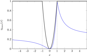
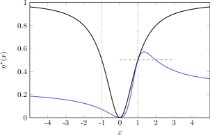
Figure 5: Bounds on benchmark parameters for the performance of the isothermal, thermoelectric engine as functions of the asymmetry parameter $x$. The right panel shows the maximum efficiency $\eta_{{{\rm max}}}(x)$ (see (84)), the left one efficiency at maximum power $\eta^{\ast}(x)$ (see (85)). The black lines follow from the bare second law, the blue lines from the stronger constraint (74). Both, $\eta_{{{\rm max}}}(x)$ and $\eta^{\ast}(x)$ asymptotically reach the value $1/4$. The dashed line in the right plot marks the value $1/2$ of $\eta^{\ast}(x)$ at the symmetric value $x=1$.

In the next step we explore the implications of (74) for the performance of the isothermal engine. To this end, we identify the output power of the device as

$$P_{{{\rm out}}}\equiv-\Delta\mu_{2}J^{\rho}_{2}=-T\mathcal{F}^{\rho}_{2}J^{\rho}_{2}$$ (75)

and correspondingly the input power as

$$P_{{{\rm in}}}\equiv\Delta\mu_{3}J^{\rho}_{3}=T\mathcal{F}^{\rho}_{3}J^{\rho}_{3}.$$ (76)

Consequently, the efficiency of the isothermal engine reads

$$\eta=\frac{P_{{{\rm out}}}}{P_{{{\rm in}}}}=-\frac{\mathcal{F}^{\rho}_{2}J^{\rho}_{2}}{\mathcal{F}^{\rho}_{3}J^{\rho}_{3}}.$$ (77)

We note that, in the situation considered here, the entropy production (12) reduces to

$$\dot{S}=\mathcal{F}^{\rho}_{2}J^{\rho}_{2}+\mathcal{F}^{\rho}_{3}J^{\rho}_{3}$$ (78)

and thus the second law $\dot{S}\geq 0$ requires $\eta\leq 1$ for isothermal engines [22].

Optimizing $\eta$ and $P_{{{\rm out}}}$ (under the condition $J_{3}^{\rho}>0$) with respect to $\mathcal{F}_{2}^{\rho}$ while keeping $\mathcal{F}_{3}^{\rho}$ fixed yields the maximum efficiency

$$\eta_{{{\rm max}}}(x,y)=x\frac{\sqrt{y+1}-1}{\sqrt{y+1}+1}$$ (79)

and the efficiency at maximum power

$$\eta^{\ast}(x,y)=\frac{xy}{4+2y},$$ (80)

where we have introduced the dimensionless parameters

$$y\equiv\frac{L_{23}L_{32}}{L_{22}L_{33}-L_{23}L_{32}}\qquad{{\rm and}}\qquad x\equiv\frac{L_{23}}{L_{32}}$$ (81)

analogous to (42). Using these definitions, the bound (74) translates to

$$\begin{array}[]{lll}h(x)\leq y\leq 0&{{\rm if}}&x<0,\\ 0\leq y\leq h(x)&{{\rm if}}&x>0\end{array}$$ (82)

with

$$h(x)=\frac{x}{(x-1)^{2}}$$ (83)

and $\eta_{{{\rm max}}}(x,y)$ as well as $\eta^{\ast}(x,y)$ attain their respective maxima with respect to $y$ at $y^{\ast}=h(x)$. The resulting bounds

$$\eta_{{{\rm max}}}(x)\equiv\eta_{{{\rm max}}}(x,y^{\ast}(x))=x\frac{\sqrt{x^{2}-x+1}-|x-1|}{\sqrt{x^{2}-x+1}+|x-1|}$$ (84)

and

$$\eta^{\ast}(x)\equiv\eta^{\ast}(x,y^{\ast}(x))=\frac{x^{2}}{4x^{2}-6x+4}$$ (85)

are plotted in figure (5). We observe that the $\eta_{{{\rm max}}}(x)$ reaches $1$ only for $x=1$ and decreases rapidly as the asymmetry parameter $x$ deviates from $1$, while $\eta^{\ast}(x)$ exceeds the Curzon-Ahlborn value $1/2$ for $x$ between $1$ and $2$ with a global maximum $\eta^{\ast\ast}=4/7$ at $x=4/3$. In contrast to the non-isothermal engines analyzed in the preceding sections, all these bounds do not depend on the number of probe terminals.

4.4 Absorption Refrigerator

By an absorption refrigerator, one commonly understands a device that generates a heat current cooling a hot reservoir, while itself being supplied by a heat source [23, 24]. The multi-terminal model allows to implement such a device by following a very similar strategy like the one used for the isothermal engine, i.e., we put $\mathcal{F}_{2}^{\rho}=\dots=\mathcal{F}_{n}^{\rho}=0$ and end up with the reduced system of phenomenological equations

$$\left(\!\begin{array}[]{c}J_{2}^{q}\\ \vdots\\ J_{n}^{q}\end{array}\!\right)=\left(\!\begin{array}[]{ccc}(\mathbb{L}_{22})_{22}&\cdots&(\mathbb{L}_{2n})_{22}\\ \vdots&\ddots&\vdots\\ (\mathbb{L}_{2n})_{22}&\cdots&(\mathbb{L}_{nn})_{22}\end{array}\!\right)\left(\!\begin{array}[]{c}\mathcal{F}_{2}^{q}\\ \vdots\\ \mathcal{F}_{n}^{q}\end{array}\!\right)$$ (86)

connecting the heat currents with the temperature gradients. Assuming the terminals $4,\dots,n$ to be pure probe terminals then leads to

$$\left(\!\begin{array}[]{c}J_{2}^{q}\\ J_{3}^{q}\end{array}\!\right)=\mathbb{L}^{{{\rm AR}}}\left(\!\begin{array}[]{c}\mathcal{F}^{q}_{2}\\ \mathcal{F}_{3}^{q}\end{array}\!\right),$$ (87)

where $\mathcal{F}_{2}^{q}<0$, $\mathcal{F}_{3}^{q}>0$ have to be adjusted such that $J^{2}_{q}>0$ and $J^{3}_{q}>0$. The matrix $\mathbb{L}^{\rm AR}$ is given by

$$\mathbb{L}^{{{\rm AR}}} =\left.\left(\!\begin{array}[]{ccc}(\mathbb{L}_{22})_{22}&\cdots&(\mathbb{L}_{2n})_{22}\\ \vdots&\ddots&\vdots\\ (\mathbb{L}_{2n})_{22}&\cdots&(\mathbb{L}_{nn})_{22}\end{array}\!\right)\right/\left(\!\begin{array}[]{ccc}(\mathbb{L}_{44})_{22}&\cdots&(\mathbb{L}_{4n})_{22}\\ \vdots&\ddots&\vdots\\ (\mathbb{L}_{4n})_{22}&\cdots&(\mathbb{L}_{nn})_{22}\end{array}\!\right)$$ (94)

$$\equiv\left(\!\begin{array}[]{cc}L_{22}^{\prime}&L_{23}^{\prime}\\ L_{32}^{\prime}&L_{33}^{\prime}\end{array}\!\right)$$ (97)

and by following the reasoning of the last section, we can derive the bound

$$4L_{22}^{\prime}L_{33}^{\prime}-\left(L_{23}^{\prime}+L_{32}^{\prime}\right)^{2}\leq 3\left(L_{23}^{\prime}-L_{32}^{\prime}\right)^{2}.$$ (98)

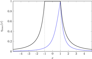
Figure 6: Maximum efficiency $\eta_{{{\rm max}}}(x)$ (see (100)) of the thermoelectric absorption refrigerator as a function of $x$. The blue line follows by virtue of the constraint (98), the black line by invoking only the second law.

The efficiency of the absorption refrigerator can be consistently defined as

$$\eta\equiv-\frac{\Delta T_{2}J_{2}^{q}}{\Delta T_{3}J^{q}_{3}}=-\frac{\mathcal{F}^{q}_{2}J^{q}_{2}}{\mathcal{F}^{q}_{3}J^{q}_{3}}\leq 1.$$ (99)

Just like for the isothermal engine, after maximizing this efficiency over $\mathcal{F}_{2}^{q}$ (under the condition $J_{2}^{q}>0$), we can derive an upper bound

$$\eta_{{{\rm max}}}(x)\equiv\frac{1}{x}\frac{\sqrt{x^{2}-x+1}-|x-1|}{\sqrt{x^{2}-x+1}+|x-1|}$$ (100)

from (98). Again, this bound is independent of the number of probe terminals. Figure 6 shows it as a function of the asymmetry parameter $x\equiv L_{23}^{\prime}/L_{32}^{\prime}$.

For completeness, we emphasize that the efficiency (99) used here differs from the coefficient of performance

$$\varepsilon\equiv\frac{J^{q}_{2}}{J^{q}_{3}}=\frac{L^{\prime}_{22}\mathcal{F}^{q}_{2}+L^{\prime}_{23}\mathcal{F}_{3}^{q}}{L^{\prime}_{32}\mathcal{F}^{q}_{2}+L^{\prime}_{33}\mathcal{F}^{q}_{3}}$$ (101)

used as a benchmark parameter in [23] and [24]. Since $\varepsilon$ is unbounded in the linear response regime, maximization with respect to $\mathcal{F}^{q}_{2}$ or $\mathcal{F}^{q}_{3}$ would be meaningless.

5 Conclusion and Outlook

We have studied the influence of broken time reversal symmetry on thermoelectric transport within the quite general framework of an $n$-terminal model. Our analytical calculations prove that the asymmetry index of any principal submatrix of the full Onsager matrix defined in (5) is bounded according to (25). This somewhat abstract bound can be translated into the set (31) of new constraints on the kinetic coefficients. Any of these constraints is obviously stronger than the bare second law and can not be deduced from Onsagers time reversal argument. Furthermore, we note that it is straight forward to repeat the procedure carried out in section 3.2 for larger principal submatrices, thus obtaining relations analogous to (31), which involve successively higher order products of kinetic coefficients. Investigating this hierarchy of constraints will be left to future work.

After the general analysis of the transport processes in the full multi-terminal set-up, we investigated the consequences of our new bounds on the performance of the model if operated as a thermoelectric heat engine. We found that both the maximum efficiency as well as the efficiency at maximum power are subject to bounds, which strongly depend on the number $n$ of terminals. In the minimal case $n=3$, we recover the strong bounds already discussed in [16]. Although our new bounds become successively weaker as $n$ is increased, they prove that reversible transport is impossible in any situation with a finite number of terminals. Only in the limit $n\rightarrow\infty$ we are back at the situation discussed by Benenti et al[9], in which the second law effectively is the only constraint. We recall that for $n=3$ our bounds can indeed be saturated as Balachandran et al[17] have shown within a specific model. Whether or not it is possible to saturate the bounds for higher $n$ remains open at this stage and constitutes an important question for future investigations.

Like in the case of the heat engine, the bound on the maximum coefficient of performance we derived for the thermoelectric refrigerator becomes weaker as $n$ increases. Interestingly, the situation is quite different for the isothermal engine and the absorption refrigerator considered in the sections 4.3 and 4.4. The bounds on the respective benchmark parameters equal those of the three-terminal case irrespective of the actual number of terminals involved. If one assumed that any kind of inelastic scattering could be simulated by a sufficiently large number of probe terminals, one had to conclude that the results shown in figures 5 and 6 were a universal bound on the efficiency of any such device. At least, the results of sections 4.3 and 4.4 suggest a fundamental difference between transport processes under broken time-reversal symmetry that are driven by only one type of affinities, i.e., either chemical potential differences or temperature differences, and those, which are induced by both types of thermodynamic forces.

We emphasize that technically all our results ultimately rely on the sum rules (8) for the elements of the transmission matrix. These constraints reflect the fundamental law of current conservation, which should be seen as the basic physical principle behind our bounds. Therefore the validity of these bounds is not limited to the quantum realm. It rather extends to any model, quantum or classical, for which the kinetic coefficients can be expressed in the generic form (6). Some specific examples for quantum mechanical models which fulfil this requirement are discussed in [17] and [25]. A classical model belonging to this class was recently introduced by Horvat et al[26].

In summary, we have achieved a fairly complete picture of thermoelectric transport under broken time reversal symmetry in systems with non-interacting particles for which the Onsager coefficients can be expressed in the Landauer-Büttiker form (6). However, fully interacting systems, which require to go beyond the single particle picture, are not covered by our analysis yet. Exploring these systems remains one of the major challenges for future research.

Appendix A Quantifying the asymmetry of positive semi-definite matrices

We first recall the definition (15)

$$\mathcal{S}(\mathbb{A})\equiv\min\left\{\left.s\in\mathbb{R}\right|\forall\mathbf{z}\in\mathbb{C}^{m}\;\;\;\mathbf{z}^{\dagger}\left(s\left(\mathbb{A}+\mathbb{A}^{t}\right)+i\left(\mathbb{A}-\mathbb{A}^{t}\right)\right)\mathbf{z}\geq 0.\right\},$$ (102)

of the asymmetry index of an arbitrary positive semi-definite matrix $\mathbb{A}\in\mathbb{R}^{m\times m}$. Below, we list some of the basic properties of this quantity, which can be inferred directly from its definition.

Proposition 1 (Basic properties of the asymmetry index).

For any positive semi-definite $\mathbb{A}\in\mathbb{R}^{m\times m}$ and $\lambda>0$, we have

$$\mathcal{S}\left(\mathbb{A}\right)=\mathcal{S}\left(\lambda\mathbb{A}\right)=\mathcal{S}(\mathbb{A}^{t})$$ (103)

and

$$\mathcal{S}\left(\mathbb{A}\right)\geq 0$$ (104)

with equality if and only if $\mathbb{A}$ is symmetric. If $\mathbb{A}$ is invertible, it holds additionally

$$\mathcal{S}\left(\mathbb{A}\right)=\mathcal{S}(\mathbb{A}^{-1}).$$ (105)

Furthermore, we can easily prove the following two propositions, which are crucial for the derivation of our main results.

Proposition 2 (Convexity of the asymmetry index).

Let $\mathbb{A},\mathbb{B}\in\mathbb{R}^{m\times m}$ be positive semi-definite, then

$$\mathcal{S}\left(\mathbb{A}+\mathbb{B}\right)\leq\max\left\{\mathcal{S}\left(\mathbb{A}\right),\mathcal{S}\left(\mathbb{B}\right)\right\}.$$ (106)

Proof.

By definition 102 the matrices

$$\mathbb{J}(s)\equiv s(\mathbb{A}+\mathbb{A}^{t})+i(\mathbb{A}-\mathbb{A}^{t})\quad{{\rm and}}\quad\mathbb{K}(s)\equiv s(\mathbb{B}+\mathbb{B}^{t})+i(\mathbb{B}-\mathbb{B}^{t})$$ (107)

with $s\equiv\max\left\{\mathcal{S}\left(\mathbb{A}\right),\mathcal{S}\left(\mathbb{B}\right)\right\}$ both are positive semi-definite. It follows that

$$\mathbb{J}(s)+\mathbb{K}(s)=s\left(\mathbb{A}+\mathbb{B}\right)+s\left(\mathbb{A}+\mathbb{B}\right)^{t}+i\left(\mathbb{A}+\mathbb{B}\right)-i\left(\mathbb{A}+\mathbb{B}\right)^{t}$$ (108)

is also positive semi-definite and hence $\mathcal{S}\left(\mathbb{A}+\mathbb{B}\right)\leq s$. ∎

Proposition 3 (Dominance of principal submatrices).

Let $\mathbb{A}\in\mathbb{R}^{m\times m}$ be positive semi-definite and $\bar{\mathbb{A}}\in\mathbb{R}^{p\times p}$ $(p<m)$ a principal submatrix of $\mathbb{A}$, then

$$\mathcal{S}(\bar{\mathbb{A}})\leq\mathcal{S}\left(\mathbb{A}\right).$$ (109)

Proof.

By definition 102

$$\mathbb{K}(s)\equiv\mathcal{S}\left(\mathbb{A}\right)(\mathbb{A}+\mathbb{A}^{t})+i(\mathbb{A}-\mathbb{A}^{t})$$ (110)

is positive semi-definite. Consequently the matrix

$$\bar{\mathbb{K}}(s)\equiv\mathcal{S}(\mathbb{A})(\bar{\mathbb{A}}+\bar{\mathbb{A}}^{t})+i(\bar{\mathbb{A}}-\bar{\mathbb{A}}^{t}),$$ (111)

which constitutes a principal submatrix of $\mathbb{K}$, is also positive semi-definite and therefore $\mathcal{S}(\bar{\mathbb{A}})\leq\mathcal{S}\left(\mathbb{A}\right)$. ∎

Appendix B Bound on the asymmetry index for special classes of matrices

Theorem 1.

Let $\mathbb{P}\in\left\{0,1\right\}^{m\times m}$ be a permutation matrix and $\mathbbm{1}$ the identity matrix, then the matrix $\mathbbm{1}-\mathbb{P}$ is positive semi-definite on $\mathbb{R}^{m}$ and its asymmetry index fulfils

$$\mathcal{S}\left(\mathbbm{1}-\mathbb{P}\right)\leq\cot\left(\frac{\pi}{m}\right).$$ (112)

Proof.

We first show that $\mathbbm{1}-\mathbb{P}$ is positive semi-definite. To this end, we note that the matrix elements of $\mathbb{P}$ are given by $\left(\mathbb{P}\right)_{ij}=\delta_{i\pi(j)}$, where $\pi\in S_{m}$ is the unique permutation associated with $\mathbb{P}$ and $S_{m}$ the symmetric group on the set $\left\{1,\dots,m\right\}$. Now, with $\mathbf{x}\equiv\left(x_{1},\dots,x_{m}\right)^{t}\in\mathbb{R}^{m}$ we have

$$\mathbf{x}^{t}\left(\mathbbm{1}-\mathbb{P}\right)\mathbf{x} =\sum_{i,j=1}^{m}\left(\delta_{ij}-\delta_{i\pi(j)}\right)x_{i}x_{j}=\sum_{i,j=1}^{m}\frac{\delta_{i\pi(j)}}{2}\left(x_{i}^{2}+x_{j}^{2}-2x_{i}x_{j}\right)$$ (113)

$$=\sum_{i,j=1}^{m}\frac{\delta_{i\pi(j)}}{2}\left(x_{i}-x_{j}\right)^{2}\geq 0.$$ (114)

We now turn to the second part of Theorem 1. For any $\mathbf{z}\equiv(z_{1},\dots,z_{m})\in\mathbb{C}^{m}$ and $s\geq 0$, we define the quadratic form

$$Q(\mathbf{z},s) \equiv\mathbf{z}^{\dagger}\left(s\left(\mathbbm{1}-\mathbb{P}\right)+s\left(\mathbbm{1}-\mathbb{P}\right)^{t}+i\left(\mathbbm{1}-\mathbb{P}\right)-i\left(\mathbbm{1}-\mathbb{P}\right)^{t}\right)\mathbf{z}$$ (115)

$$=\mathbf{z}^{\dagger}\left(2s\cdot\mathbbm{1}-(s+i)\mathbb{P}-(s-i)\mathbb{P}^{t}\right)\mathbf{z}.$$ (116)

By definition 102 the minimum $s$, for which $Q(\mathbf{z},s)$ is positive semi-definite, equals the asymmetry index of $\mathbbm{1}-\mathbb{P}$. This observation enables us to derive an upper bound for $\mathcal{S}\left(\mathbbm{1}-\mathbb{P}\right)$. To this end, we make use of the cycle decomposition

$$\pi=\left(i_{1},\pi(i_{1}),\dots,\pi^{n_{1}-1}(i_{1})\right)\dots\left(i_{k},\pi(i_{k}),\dots,\pi^{n_{k}-1}(i_{k})\right)$$ (117)

of $\pi$, where $i_{1},\dots,i_{k}\in\left\{1,\dots,m\right\}$, $\pi^{l}(i)$ is defined recursively by

$$\pi^{l}(i)\equiv\pi\left(\pi^{l-1}(i)\right)\qquad{{\rm and}}\qquad\pi^{0}(i)=i,$$ (118)

$k$ denotes the number of independent cycles of and $n_{r}$ the length the $r^{{{\rm th}}}$ cycle. By virtue of this decomposition, (115) can be rewritten as

$$Q(\mathbf{z},s) =\sum_{i,j=1}^{m}\left(2s\delta_{ij}-(s+i)\delta_{i\pi(j)}-(s-i)\delta_{\pi(i)j}\right)z_{i}^{\ast}z_{j}$$ (119)

$$=\sum_{i=1}^{m}2sz_{i}^{\ast}z_{i}-(s+i)z_{\pi(i)}^{\ast}z_{i}-(s-i)z_{i}^{\ast}z_{\pi(i)}$$

$$=\sum_{r=1}^{k}\sum_{l_{r}=0}^{n_{r}-1}2sz^{\ast}[\pi^{l_{r}}(i_{r})]z[\pi^{l_{r}}(i_{r})]$$

$$\hskip 113.81102pt-(s+i)z^{\ast}[\pi^{l_{r}+1}(i_{r})]z[\pi^{l_{r}}(i_{r})]$$

$$\hskip 113.81102pt-(s-i)z^{\ast}[\pi^{l_{r}}(i_{r})]z[\pi^{l_{r}+1}(i_{r})],$$ (121)

where, for convenience, we introduced the notation $z[x]\equiv z_{x}$. Next, we define the vectors $\tilde{\mathbf{z}}_{r}\in\mathbb{C}^{n_{r}}$ with elements $\left(\tilde{\mathbf{z}}_{r}\right)_{j}\equiv z\left[\pi^{j-1}(i_{r})\right]$ and the Hermitian matrices $\mathbb{H}_{n_{r}}(s)\in\mathbb{C}^{n_{r}\times n_{r}}$ with matrix elements

$$\left(\mathbb{H}_{n_{r}}(s)\right)_{ij}\equiv 2s\delta_{ij}-(s+i)\delta_{ij+1}-(s-i)\delta_{i+1j},$$ (122)

where periodic boundary conditions $n_{r}+1=1$ for the indices $i,j=1,\dots,n_{r}$ are understood. These definitions allow us to cast (121) in the rather compact form

$$Q(\mathbf{z},s)=\sum_{r=1}^{k}\tilde{\mathbf{z}}_{r}^{\dagger}\mathbb{H}_{n_{r}}(s)\tilde{\mathbf{z}}_{r}.$$ (123)

Obviously, any value of $s$ for which all the $\mathbb{H}_{n_{r}}(s)$ are positive semi-definite serves as a lower bound for $\mathcal{S}\left(\mathbbm{1}-\mathbb{P}\right)$. Moreover, we can calculate the eigenvalues of $\mathbb{H}_{n_{r}}(s)$ explicitly. Inserting the Ansatz $\mathbf{v}\equiv(v_{1},\dots,v_{n_{r}})^{t}\in\mathbb{C}^{n_{r}}$ into the eigenvalue equation

$$\mathbb{H}_{n_{r}}(s)\mathbf{v}=\lambda\mathbf{v}\qquad(\lambda\in\mathbb{R})$$ (124)

yields

$$\lambda v_{j}=2sv_{j}-(s+i)v_{j-1}-(s-i)v_{j+1},$$ (125)

where again periodic boundary conditions $v_{n_{r}+1}=v_{1}$ are understood. This recurrence equation can be solved by standard techniques. We put $v_{j}\equiv\exp\left(2\pi i\kappa j/n_{r}\right)$ with $(\kappa=1,\dots,n_{r})$ and obtain the eigenvalues

$$\lambda_{\kappa}=2\left(s-s\cos\left(\frac{2\pi\kappa}{n_{r}}\right)-\sin\left(\frac{2\pi\kappa}{n_{r}}\right)\right).$$ (126)

For any fixed $s\geq 0$, the function

$$f(x,s)\equiv s-s\cos x-\sin x$$ (127)

is non-negative for $x\in[x^{\ast},2\pi]$ and strictly negative for $x\in(0,x^{\ast})$ with

$$x^{\ast}\equiv\arccos\left(\frac{s^{2}-1}{s^{2}+1}\right).$$ (128)

Therefore, all the eigenvalues $\lambda_{\kappa}$ of $\mathbb{H}_{n_{r}}(s)$ are non-negative, if and only if

$$\frac{2\pi}{n_{r}}\geq\arccos\left(\frac{s^{2}-1}{s^{2}+1}\right).$$ (129)

Solving (129) for $s$ gives the equivalent condition

$$s\geq\cot\left(\frac{\pi}{n_{r}}\right).$$ (130)

Since $n_{r}\leq m$ and therefore $2\pi/n_{r}\geq 2\pi/m$, we can conclude that any of the $\mathbb{H}_{n_{r}}(s)$ is positive semi-definite for any

$$s\geq\cot\left(\frac{\pi}{m}\right),$$ (131)

thus establishing the desired result (112).
∎

Corollary 1.

Let $\mathbb{T}\in\mathbb{R}^{m\times m}$ be doubly stochastic, then the matrix $\mathbbm{1}-\mathbb{T}$ is positive semi-definite and its asymmetry index fulfils

$$\mathcal{S}\left(\mathbbm{1}-\mathbb{T}\right)\leq\cot\left(\frac{\pi}{m}\right).$$ (132)

Proof.

The Birkhoff-theorem (see p. 549 in [27]) states that for any doubly stochastic matrix $\mathbb{T}\in\mathbb{R}^{m\times m}$ there is a finite number of permutation matrices $\mathbb{P}_{1},\dots\mathbb{P}_{N}\in\{0,1\}^{m\times m}$ and positive scalars $\lambda_{1},\dots,\lambda_{N}\in\mathbb{R}$ such that

$$\sum_{k=1}^{N}\lambda_{k}=1\qquad{{\rm and}}\qquad\sum_{k=1}^{N}\lambda_{k}\mathbb{P}_{k}=\mathbb{T}.$$ (133)

Hence, we have

$$\mathbbm{1}-\mathbb{T}=\sum_{k=1}^{N}\lambda_{k}\left(\mathbbm{1}-\mathbb{P}_{k}\right)$$ (134)

and consequently $\mathbbm{1}-\mathbb{T}$ must be positive semi-definite by virtue of Theorem 1. Furthermore, using Proposition 2 and again Theorem 1 gives the bound (132). ∎

Theorem 2.

Let $\bar{\mathbb{P}}\in\left\{0,1\right\}^{m\times m}$ be a partial permutation matrix, i.e., any row and column of $\bar{\mathbb{P}}$ contains at most one non-zero entry and all of these non-zero entries are $1$. Then, the matrix $\mathbbm{1}-\bar{\mathbb{P}}$ is positive semi-definite and its asymmetry index fulfils

$$\mathcal{S}\left(\mathbbm{1}-\bar{\mathbb{P}}\right)\leq\cot\left(\frac{\pi}{m+1}\right).$$ (135)

Proof.

Let $q$ be the number of non-vanishing entries of $\bar{\mathbb{P}}$. If $q=0$, $\bar{\mathbb{P}}$ equals the zero matrix and there is nothing to prove. If $q=m$, $\bar{\mathbb{P}}$ itself must be a permutation matrix and Lemma 1 provides that $\mathbbm{1}-\bar{\mathbb{P}}$ is positive semi-definite as well as the bound

$$\mathcal{S}\left(\mathbbm{1}-\bar{\mathbb{P}}\right)\leq\cot\left(\frac{\pi}{m}\right),$$ (136)

which is even stronger than (135). If $0<q<m$, there are two index sets $A\subset\{1,\dots,m\}$ and $B\subset\{1,\dots,m\}$ of equal cardinality $m-q$, such that the rows of $\bar{\mathbb{P}}$ indexed by $A$ and the columns of $\bar{\mathbb{P}}$ indexed by $B$ contain only zero entries. Clearly, in this case, $\bar{\mathbb{P}}$ is not a permutation matrix. Nevertheless, we can define a bijective map

$$\bar{\pi}:\{1,\dots,m\}\setminus B\rightarrow\{1,\dots,m\}\setminus A$$ (137)

in such a way that $\bar{\mathbb{P}}$ can be regarded as a representation of $\bar{\pi}$ . To this end, we denote by $\{\mathbf{e}_{1},\dots,\mathbf{e}_{m}\}$ the canonical basis of $\mathbb{R}^{m}$ and define $\bar{\pi}:\;i\mapsto\bar{\pi}(i)$ such that

$$\bar{\mathbb{P}}\mathbf{e}_{i}\equiv\mathbf{e}_{\bar{\pi}(i)}.$$ (138)

This definition naturally leads to the cycle decomposition

$$\bar{\pi}= \left(i_{1},\bar{\pi}(i_{1}),\dots,\bar{\pi}^{n_{1}-1}(i_{1})\right)\cdots\left(i_{k},\bar{\pi}(i_{k}),\dots,\bar{\pi}^{n_{k}-1}(i_{k})\right)$$ (139)

$$\left[j_{1},\bar{\pi}(j_{1}),\dots,\bar{\pi}^{\bar{n}_{1}-1}(j_{1})\right]\cdots\left[j_{\bar{k}},\bar{\pi}(j_{\bar{k}}),\dots,\bar{\pi}^{\bar{n}_{\bar{k}}-1}(j_{\bar{k}})\right].$$

Here, we introduced two types of cycles. The ones in round brackets, which we will term complete, are just ordinary permutation cycles, which close by virtue of the condition $\bar{\pi}^{n_{r}}(i_{r})=i_{r}$ and therefore must be contained completely in the set

$$I\equiv\left(\{1,\dots,m\}\setminus B\right)\cap\left(\{1,\dots,m\}\setminus A\right)=\{1,\dots,m\}\setminus\left(A\cup B\right).$$ (140)

The cycles in rectangular brackets, which will be termed incomplete, do not close, but begin with a certain $j_{\bar{r}}$ taken from the set

$$D\equiv\left(\{1,\dots,m\}\setminus B\right)\setminus\left(\{1,\dots,m\}\setminus A\right)=A\setminus B$$ (141)

and terminate after $\bar{n}_{\bar{r}}-1$ iterations with $\bar{\pi}^{\bar{n}_{\bar{r}}-1}(j_{\bar{r}})$, which is contained in

$$R\equiv\left(\{1,\dots,m\}\setminus A\right)\setminus\left(\{1,\dots,m\}\setminus B\right)=B\setminus A.$$ (142)

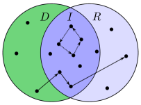
Figure 7: Schematic illustration of the cycle decomposition (139). The green circle represents the set $\{1,\dots,m\}\setminus B$, the blue one the set $\{1,\dots,m\}\setminus A$. The black dots symbolize the elements of the respective sets and the arrows show the action of the map $\bar{\pi}$. While the dashed arrows form a complete cycle, the solid ones combine to an incomplete cycle.

Figure (7) shows a schematic visualization of the two different types of cycles. We note that, since the map $\bar{\pi}$, is bijective the cycle decomposition 139 is unique up to the choice of the $i_{r}$ and any element of

$$J\equiv\left(\{1,\dots,m\}\setminus B\right)\cup\left(\{1,\dots,m\}\setminus A\right)=\{1,\dots,m\}\setminus\left(A\cap B\right)$$ (143)

shows up exactly once.

For the next step, we introduce the vectors

$$\mathbf{a}\equiv\sum_{i\in A}\mathbf{e}_{i}\qquad{{\rm and}}\qquad\mathbf{b}\equiv\sum_{i\in B}\mathbf{e}_{i},$$ (144)

as well as the bordered matrix

$$\mathbb{B}\equiv\left(\!\begin{array}[]{cc}\bar{\mathbb{P}}&\mathbf{a}\\ \mathbf{b}^{t}&1-m+q\end{array}\!\right).$$ (145)

Obviously, all rows and columns of $\mathbb{B}$ sum up to $1$ and all off-diagonal entries are non-negative. Hence, with $B_{ij}\equiv\left(\mathbb{B}\right)_{ij}$, we have for any $\mathbf{x}\in\mathbb{R}^{m}$

$$\mathbf{x}^{t}\left(\mathbbm{1}-\mathbb{B}\right)\mathbf{x} =\sum_{i,j=1}^{m}\left(\delta_{ij}-B_{ij}\right)x_{i}x_{j}=\sum_{i,j=1}^{m}\frac{B_{ij}}{2}\left(x_{i}^{2}+x_{j}^{2}-2x_{i}x_{j}\right)$$ (146)

$$=\sum_{i,j=1,\;i\neq j}^{m}\frac{B_{ij}}{2}\left(x_{i}-x_{j}\right)^{2}\geq 0,$$

i.e., the matrix $\mathbbm{1}-\mathbb{B}$ is positive semi-definite. Since $\mathbbm{1}-\bar{\mathbb{P}}$ is a principal submatrix of $\mathbbm{1}-\mathbb{B}$, (146) implies in particular that $\mathbbm{1}-\bar{\mathbb{P}}$ is positive semi-definite, thus establishing the first part of Lemma 2.

We will now prove the bound (135) on the asymmetry index of $\mathbbm{1}-\bar{\mathbb{P}}$. To this end, for any $\mathbf{z}\in\mathbb{C}^{m+1}$ we associate the matrix $\mathbb{B}$ with the quadratic form

$$\bar{Q}(\mathbf{z},s) \equiv\mathbf{z}^{\dagger}\left(s(\mathbbm{1}-\mathbb{B})+s(\mathbbm{1}-\mathbb{B})^{t}+i(\mathbbm{1}-\mathbb{B})-i(\mathbbm{1}-\mathbb{B})^{t}\right)\mathbf{z}$$ (147)

$$=\mathbf{z}^{\dagger}\left(2s\cdot\mathbbm{1}-(s+i)\mathbb{B}-(s-i)\mathbb{B}^{t}\right)\mathbf{z}.$$ (148)

and notice that the minimum $s$ for which $\bar{Q}(\mathbf{z},s)$ is positive semi-definite equals the asymmetry index of $\mathbbm{1}-\mathbb{B}$. Furthermore, since $\mathbbm{1}-\bar{\mathbb{P}}$ is a principal submatrix of $\mathbbm{1}-\mathbb{B}$, Proposition 3 implies that this particular value of $s$ is also an upper bound on the asymmetry index of $\mathbbm{1}-\bar{\mathbb{P}}$. Now, by inserting the decomposition

$$\mathbf{z}\equiv\sum_{i=1}^{m+1}z_{i}\mathbf{e}_{i}$$ (149)

into (148) while keeping in mind the definition (138), we obtain

$$\bar{Q}(\mathbf{z},s) =2s\sum_{i=1}^{m}z_{i}^{\ast}z_{i}+2s(m-q)z^{\ast}_{m+1}z_{m+1}$$ (150)

$$\quad-(s+i)\left(\sum_{i\in\{1,\dots,m\}\setminus B}z^{\ast}_{\bar{\pi}(i)}z_{i}+\sum_{i\in A}z_{i}^{\ast}z_{m+1}+\sum_{i\in B}z_{m+1}^{\ast}z_{i}\right)$$

$$\quad-(s-i)\left(\sum_{i\in\{1,\dots,m\}\setminus B}z^{\ast}_{i}z_{\bar{\pi}(i)}+\sum_{i\in A}z_{m+1}^{\ast}z_{i}+\sum_{i\in B}z_{i}^{\ast}z_{m+1}\right).$$

By realizing

$$A=D\cup\left(A\cap B\right),\quad B=R\cup\left(A\cap B\right),\quad\{1,\dots,m\}=J\cup\left(A\cap B\right)$$ (151)

and making use of the cycle decomposition (139), we can rewrite (150) as

$$\bar{Q}(\mathbf{z},s)=2s\sum_{r=1}^{k}\sum_{l_{r}=0}^{n_{r}-1}z^{\ast}[\bar{\pi}^{l_{r}}(i_{r})]z[\bar{\pi}^{l_{r}}(i_{r})]+2s\sum_{{\bar{r}}=1}^{\bar{k}}\sum_{l_{\bar{r}}=0}^{n_{\bar{r}}-1}z^{\ast}[\bar{\pi}^{l_{\bar{r}}}(j_{\bar{r}})]z[\bar{\pi}^{l_{\bar{r}}}(j_{\bar{r}})]$$

$$+2s\sum_{i\in A\cap B}z_{i}^{\ast}z_{i}+2s(m-q)z^{\ast}_{m+1}z_{m+1}$$

$$-(s+i)\left(\sum_{r=1}^{k}\sum_{l_{r}=0}^{n_{r}-1}z^{\ast}[\bar{\pi}^{l_{r}+1}(i_{r})]z[\bar{\pi}^{l_{r}}(i_{r})]+\sum_{\bar{r}=1}^{\bar{k}}\sum_{l_{\bar{r}}=0}^{n_{\bar{r}}-2}z^{\ast}[\bar{\pi}^{l_{\bar{r}}+1}(j_{\bar{r}})]z[\bar{\pi}^{l_{\bar{r}}}(j_{\bar{r}})]\right.$$

$$\left.\hskip 85.35826pt+\sum_{i\in D}z_{i}^{\ast}z_{m+1}+\sum_{i\in R}z^{\ast}_{m+1}z_{i}+\sum_{i\in A\cap B}\left(z_{i}^{\ast}z_{m+1}+z_{m+1}^{\ast}z_{i}\right)\right)$$

$$-(s-i)\left(\sum_{r=1}^{k}\sum_{l_{r}=0}^{n_{r}-1}z^{\ast}[\bar{\pi}^{l_{r}}(i_{r})]z[\bar{\pi}^{l_{r}+1}(i_{r})]+\sum_{\bar{r}=1}^{\bar{k}}\sum_{l_{\bar{r}}=0}^{n_{\bar{r}}-2}z^{\ast}[\bar{\pi}^{l_{\bar{r}}}(j_{\bar{r}})]z[\bar{\pi}^{l_{\bar{r}}+1}(j_{\bar{r}})]\right.$$

$$\left.\hskip 85.35826pt+\sum_{i\in D}z_{m+1}^{\ast}z_{i}+\sum_{i\in R}z^{\ast}_{i}z_{m+1}+\sum_{i\in A\cap B}\left(z_{m+1}^{\ast}z_{i}+z_{i}^{\ast}z_{m+1}\right)\right),$$

(152)

thus explicitly separating contributions from complete and incomplete cycles. Finally, since we have

$$\sum_{i\in D}z_{i}^{\ast}z_{m+1}=\sum_{\bar{r}=1}^{\bar{k}}z^{\ast}[j_{\bar{r}}]z_{m+1},\quad \sum_{i\in R}z_{m+1}^{\ast}z_{i}=\sum_{\bar{r}=1}^{\bar{k}}z^{\ast}_{m+1}z[\bar{\pi}^{n_{\bar{r}}-1}(j_{\bar{r}})],$$ (153)

$$\sum_{i\in D}z_{m+1}^{\ast}z_{i}=\sum_{\bar{r}=1}^{\bar{k}}z^{\ast}_{m+1}z[j_{\bar{r}}],\quad \sum_{i\in R}z_{i}^{\ast}z_{m+1}=\sum_{\bar{r}=1}^{\bar{k}}z^{\ast}[\bar{\pi}^{n_{\bar{r}}-1}_{\bar{r}}(j_{\bar{r}})]z_{m+1},$$ (154)

by employing the definitions

$$\tilde{\mathbf{z}}_{r} \equiv\left(z[i_{r}],z[\bar{\pi}(i_{r})],\dots,z[\bar{\pi}^{n_{r}-1}(i_{r})]\right)^{t}\in\mathbb{C}^{n_{r}\times n_{r}}\qquad{{\rm and}}\qquad$$ (155)

$$\tilde{\bar{\mathbf{z}}}_{\bar{r}} \equiv\left(z[j_{\bar{r}}],z[\bar{\pi}(j_{\bar{r}})],\dots,z[\bar{\pi}^{n_{\bar{r}}-1}(j_{\bar{r}})],z_{m+1}\right)^{t}\in\mathbb{C}^{(n_{\bar{r}}+1)\times(n_{\bar{r}}+1)},$$ (156)

(152) can be written as

$$\bar{Q}(\mathbf{z},s) =\sum_{r=1}^{k}\tilde{\mathbf{z}}_{r}^{\dagger}\mathbb{H}_{n_{r}}(s)\tilde{\mathbf{z}}_{r}+\sum_{\bar{r}=1}^{\bar{k}}\tilde{\bar{\mathbf{z}}}_{\bar{r}}^{\dagger}\mathbb{H}_{n_{\bar{r}}+1}(s)\tilde{\bar{\mathbf{z}}}_{\bar{r}}+2s\sum_{i\in A\cap B}\left|z_{i}-z_{m+1}\right|^{2},$$ (157)

where the matrices $\mathbb{H}_{n}(s)$ are defined in (122). Since we have already shown for the proof of Lemma 1 that $\mathbb{H}_{n}(s)$ is positive semi-definite for any $s\geq\cot\left(\pi/n\right)$, we immediately infer from (157) that $\bar{Q}(\mathbf{z},s)$ is positive semi-definite for any

$$s\geq\cot\left(\frac{\pi}{{{\rm max}}\{n_{r},n_{\bar{r}}+1\}}\right).$$ (158)

Since $\max\{n_{r},n_{\bar{r}}+1\}\leq m+1$, we finally end up with

$$\mathcal{S}\left(\mathbbm{1}-\bar{\mathbb{P}}\right)\leq\mathcal{S}\left(\mathbbm{1}-\mathbb{B}\right)\leq\cot\left(\frac{\pi}{m+1}\right).$$ (159)

∎

Corollary 2.

Let $\bar{\mathbb{T}}\in\mathbb{R}^{m\times m}$ be doubly substochastic, then the matrix $\mathbbm{1}-\bar{\mathbb{T}}$ is positive semi-definite and its asymmetry index fulfils

$$\mathcal{S}\left(\mathbbm{1}-\bar{\mathbb{T}}\right)\leq\cot\left(\frac{\pi}{m+1}\right).$$ (160)

Proof.

It can be shown that any doubly substochastic matrix is the convex combination of a finite number of partial permutation matrices $\bar{\mathbb{P}}_{k}$ (see p. 165 in [28]), i.e., we have

$$\bar{\mathbb{T}}=\sum_{k=1}^{N}\lambda_{k}\bar{\mathbb{P}}_{k}$$ (161)

with

$$\lambda_{k}>0\qquad{{\rm and}}\qquad\sum_{k=1}^{N}\lambda_{k}=1.$$ (162)

Consequently, it follows

$$\mathbbm{1}-\bar{\mathbb{T}}=\sum_{k=1}^{N}\lambda_{k}\left(\mathbbm{1}-\bar{\mathbb{P}}\right).$$ (163)

Using the same argument with Lemma 2 instead of Lemma 1 in the proof of Corollary 1 completes the proof of Corollary 2 . ∎

Appendix C Bound on the asymmetry index of the Schur complements

For $\mathbb{A}\in\mathbb{C}^{m\times m}$ partitioned as

$$\mathbb{A}\equiv\left(\!\begin{array}[]{cc}\mathbb{A}_{11}&\mathbb{A}_{12}\\ \mathbb{A}_{21}&\mathbb{A}_{22}\end{array}\!\right)$$ (164)

with non-singular $\mathbb{A}_{22}\in\mathbb{R}^{p\times p}$, the Schur complement of $\mathbb{A}_{22}$ in $\mathbb{A}$ is defined by (see p. 18 in [29])

$$\mathbb{A}/\mathbb{A}_{22}=\mathbb{A}_{11}-\mathbb{A}_{12}\mathbb{A}_{22}^{-1}\mathbb{A}_{21}.$$ (165)

Regarding the asymmetry index, we have the following proposition.

Proposition 4 (Dominance of the Schur complement).

Let $\mathbb{A}\in\mathbb{R}^{m\times m}$ be a positive semi-definite matrix partitioned as in (164), where $\mathbb{A}_{22}\in\mathbb{R}^{p\times p}$ is non-singular, then the matrix $\mathbb{A}/\mathbb{A}_{22}$ is positive semi-definite and its asymmetry index fulfils

$$\mathcal{S}\left(\mathbb{A}/\mathbb{A}_{22}\right)\leq\mathcal{S}\left(\mathbb{A}\right).$$ (166)

Proof.

By assumption and by definition 102, we have for any $\mathbf{z}\in\mathbb{C}^{m}$

$$\mathbf{z}^{\dagger}\mathbb{A}\mathbf{z}\geq 0\qquad{{\rm and}}\qquad\mathbf{z}^{\dagger}\left(\mathcal{S}\left(\mathbb{A}\right)(\mathbb{A}+\mathbb{A}^{t})+i(\mathbb{A}-\mathbb{A}^{t})\right)\mathbf{z}\geq 0.$$ (167)

Putting

$$\mathbf{z}\equiv\left(\!\begin{array}[]{c}\mathbf{z}_{p}\\ -\mathbb{A}_{22}^{-1}\mathbb{A}_{21}\mathbf{z}_{p}\end{array}\!\right)\qquad{{\rm with}}\qquad\mathbf{z}_{p}\in\mathbb{C}^{p}$$ (168)

yields

$$\mathbf{z}_{p}^{\dagger}\left(\mathbb{A}/\mathbb{A}_{22}\right)\mathbf{z}_{p}\geq 0$$ (169)

and

$$\mathbf{z}_{p}^{\dagger}\left(\mathcal{S}\left(\mathbb{A}\right)(\mathbb{A}/\mathbb{A}_{22}+(\mathbb{A}/\mathbb{A}_{22})^{t})+i(\mathbb{A}/\mathbb{A}_{22}-(\mathbb{A}/\mathbb{A}_{22})^{t})\right)\mathbf{z}_{p}\geq 0.$$ (170)

∎

For the special class of matrices considered in Corollary 2, the assertion of Proposition 4 can be even strengthened. Before being able to state this stronger result, we need to prove the following Lemma.

Lemma 1.

Let $\bar{\mathbb{T}}\in\mathbb{R}^{m\times m}$ be a doubly substochastic matrix and $\mathbb{S}\equiv\mathbbm{1}-\bar{\mathbb{T}}$ be partitioned as

$$\mathbb{S}\equiv\left(\!\begin{array}[]{cc}\mathbb{S}_{11}&\mathbb{S}_{12}\\ \mathbb{S}_{21}&\mathbb{S}_{22}\end{array}\!\right),$$ (171)

where $\mathbb{S}_{22}\in\mathbb{R}^{p\times p}$ is non-singular, then there is a doubly substochastic matrix $\bar{\mathbb{T}}_{m-p}\in\mathbb{R}^{(m-p)\times(m-p)}$, such that

$$\mathbb{S}/\mathbb{S}_{22}=\mathbbm{1}-\bar{\mathbb{T}}_{m-p}.$$ (172)

Proof.

We start with the case $p=1$. Let $\bar{T}_{ij}$ be the matrix elements of $\bar{\mathbb{T}}$, then the matrix elements of $\mathbb{S}/\mathbb{S}_{22}$ are given by

$$\left(\mathbb{S}/\mathbb{S}_{22}\right)_{kl}\equiv\delta_{kl}-\bar{T}_{kl}-\frac{\bar{T}_{km}\bar{T}_{ml}}{1-\bar{T}_{mm}}$$ (173)

with $k,l=1,\dots,m-1$. Obviously, we have

$$\sum_{k=1}^{m-1}\left(\mathbb{S}/\mathbb{S}_{22}\right)_{kl}=1-\sum_{k=1}^{m-1}\bar{T}_{kl}-\frac{\bar{T}_{ml}}{1-\bar{T}_{mm}}\sum_{k=1}^{m-1}\bar{T}_{km}\leq 1.$$ (174)

Furthermore, since by assumption

$$\sum_{i=1}^{m}\bar{T}_{ij}\leq 1$$ (175)

it follows

$$\sum_{k=1}^{m-1}\left(\mathbb{S}/\mathbb{S}_{22}\right)_{kl}\geq 1-(1-\bar{T}_{ml})-\frac{\bar{T}_{ml}(1-\bar{T}_{mm})}{1-\bar{T}_{mm}}=0.$$ (176)

Analogously, we find

$$0\leq\sum_{l=1}^{m-1}\left(\mathbb{S}/\mathbb{S}_{22}\right)_{kl}\leq 1.$$ (177)

Next, we investigate the sign pattern of the $\left(\mathbb{S}/\mathbb{S}_{22}\right)_{kl}$. First, for $k\neq l$, we have

$$\left(\mathbb{S}/\mathbb{S}_{22}\right)_{kl}=-\bar{T}_{kl}-\frac{\bar{T}_{km}\bar{T}_{ml}}{1-\bar{T}_{mm}}\leq 0.$$ (178)

Second, we rewrite the $\left(\mathbb{S}/\mathbb{S}_{22}\right)_{kk}$ as

$$\left(\mathbb{S}/\mathbb{S}_{22}\right)_{kk}=1-\bar{T}_{kk}-\frac{\bar{T}_{km}\bar{T}_{mk}}{1-\bar{T}_{mm}}=\frac{(1-\bar{T}_{kk})(1-\bar{T}_{mm})-\bar{T}_{km}\bar{T}_{mk}}{1-\bar{T}_{mm}}$$ (179)

The numerator appearing on the right hand side can be written as

$$(1-\bar{T}_{kk})(1-\bar{T}_{mm})-\bar{T}_{km}\bar{T}_{mk}={{\rm Det}}\left(\!\begin{array}[]{cc}1-\bar{T}_{kk}&-\bar{T}_{km}\\ -\bar{T}_{mk}&1-\bar{T}_{mm}\end{array}\!\right),$$ (180)

which is a principal minor of $\mathbbm{1}-\bar{\mathbb{T}}$. Since, by Corollary 2 is positive semi-definite, we end up with

$$0\leq\left(\mathbb{S}/\mathbb{S}_{22}\right)_{kk}\leq 1.$$ (181)

From the sum rules (174), (176) and (177) and the constraints (178) and (181), we deduce that $\mathbbm{1}-\mathbb{S}/\mathbb{S}_{22}$ is doubly substochastic and thus we have proven Lemma 1 for $p=1$. We now continue by induction. To this end, we assume that Lemma 1 is true for $p=q$. For $p=q+1$ the matrix $\mathbb{S}_{22}\in\mathbb{R}^{(q+1)\times(q+1)}$ can be partitioned as

$$\mathbb{S}_{22}\equiv\left(\!\begin{array}[]{cc}W_{11}&\mathbf{W}_{12}^{t}\\ \mathbf{W}_{21}&\mathbb{W}_{22}\end{array}\!\right)$$ (182)

with $\mathbb{W}_{22}\in\mathbb{R}^{q\times q}$, $W_{11}\in\mathbb{R}$ and accordingly $\mathbf{W}_{12},\mathbf{W}_{21}\in\mathbb{R}^{q}$. The Crabtree-Haynsworth quotient formula (see p. 25 in [29]), allows us to rewrite $\mathbb{S}/\mathbb{S}_{22}$ as

$$\mathbb{S}/\mathbb{S}_{22}=\left(\mathbb{S}/\mathbb{W}_{22}\right)/\left(\mathbb{S}_{22}/\mathbb{W}_{22}\right).$$ (183)

A direct calculation shows that $\mathbb{S}_{22}/\mathbb{W}_{22}\in\mathbb{R}$ is the lower right diagonal entry of $\mathbb{S}/\mathbb{W}_{22}$ (see p. 25 in [29] for details). Furthermore, by the induction hypothesis, there is a doubly substochastic matrix $\bar{\mathbb{T}}_{m-q}\in\mathbb{R}^{(m-q)\times(m-q)}$, such that

$$\mathbb{S}/\mathbb{W}_{22}=\mathbbm{1}-\bar{\mathbb{T}}_{m-q}.$$ (184)

Thus, (183) reduces to the case $p=1$, for which we have already proven Lemma 1. ∎

From Lemma 1 and Corollary 2, we immediately deduce

Corollary 3.

Let $\bar{\mathbb{T}}$, $\mathbb{S}$ and $\mathbb{S}_{22}$ be as in Lemma 1, then

$$\mathcal{S}\left(\mathbb{S}/\mathbb{S}_{22}\right)\leq\cot\left(\frac{\pi}{m-p+1}\right).$$ (185)

References

References

- [1] M. S. Dresselhaus, G. Chen, M. Y. Tang, R. Yang, H. Lee, D. Wang, Z. Ren, J.-P. Fleurial, and P. Gogna. New Directions for Low-Dimensional Thermoelectric Materials. Adv. Mat., 19:1043–1053, 2007.
- [2] G. J. Snyder and S. Toberer. Complex thermoelectric materials. Nature Mater., 7:105–114, 2008.
- [3] L. E. Bell. Cooling, heating, generating power, and recovering waste heat with thermoelectric systems. Science, 321:1457–61, 2008.
- [4] C. J. Vineis, A. Shakouri, A. Majumdar, and M. G. Kanatzidis. Nanostructured thermoelectrics: big efficiency gains from small features. Adv. Mat., 22:3970–80, 2010.
- [5] T. E. Humphrey and H. Linke. Quantum, cyclic, and particle-exchange heat engines. Physica E: Low-dimensional Systems and Nanostructures, 29:390–398, 2005.
- [6] G. D. Mahan, and J. O. Sofo. The best thermoelectric. Proc. Natl. Acad. Sci., 93:7436-7439, 1996.
- [7] T. E. Humphrey, R. Newbury, R. P. Taylor, and H. Linke. Reversible Quantum Brownian Heat Engines for Electrons. Phys. Rev. Lett., 89:116801, 2002.
- [8] T. E. Humphrey and H. Linke. Reversible Thermoelectric Nanomaterials. Phys. Rev. Lett., 94:096601, 2005.
- [9] G. Benenti, K. Saito, and G. Casati. Thermodynamic Bounds on Efficiency for Systems with Broken Time-Reversal Symmetry. Phys. Rev. Lett., 106:230602, 2011.
- [10] R. Landauer. Spatial Variation of Currents and Fields Due to Localized Scatterers in Metallic Conduction. IBM J. Res. Develop., 1:223, 1957.
- [11] U. Sivan and Y. Imry. Multichannel Landauer formula for thermoelectric transport with application to thermopower near the mobility edge. Phys. Rev. B, 33:551–558, 1986.
- [12] P. N. Butcher. Thermal and electrical transport formalism for electronic microstructures with many terminals. J. Phys. Condens. Matter, 2:4869–4878, 1990.
- [13] M. Büttiker. Symmetry of electrical conduction. IBM J. Res. Develop., 32:317–334, 1988.
- [14] M. Büttiker. Coherent and sequential tunneling in series barriers. IBM J. Res. Develop., 32:63–75, 1988.
- [15] K. Saito, G. Benenti, G. Casati, and T. Prosen. Thermopower with broken time-reversal symmetry. Phys. Rev. B, 84:201306(R), 2011.
- [16] K. Brandner, K. Saito, and U. Seifert. Strong Bounds on Onsager Coefficients and Efficiency for Three-Terminal Thermoelectric Transport in a Magnetic Field. Phys. Rev. Lett., 110:070603, 2013.
- [17] V. Balachandran, G. Benenti, and G. Casati. Efficiency of three-terminal thermoelectric transport under broken time-reversal symmetry. Phys. Rev. B, 87:165419, 2013.
- [18] H. B. Callen. Thermodynamics and an Introduction to Thermostatics. John Wiley & Sons, New York, 2nd edition, 1985.
- [19] J.-P. Crouzeix and C. Gutan. A Measure Of Asymmetry For Positive Semidefinite Matrices. Optimization, 52:251–262, 2003.
- [20] F. L. Curzon and B. Ahlborn. Efficiency of a Carnot engine at maximum power output. Am. J. Phys., 43:22, 1975.
- [21] M. Esposito, K. Lindenberg, and C. Van den Broeck. Universality of Efficiency at Maximum Power. Phys. Rev. Lett., 102:130602, 2009.
- [22] U. Seifert. Stochastic thermodynamics, fluctuation theorems and molecular machines. Rep. Prog. Phys., 75:126001, 2012.
- [23] J. Palao, R. Kosloff, and J. Gordon. Quantum thermodynamic cooling cycle. Phys. Rev. E, 64:056130, 2001.
- [24] P. Skrzypczyk, N. Brunner, N. Linden, and S. Popescu. The smallest refrigerators can reach maximal efficiency. J. Phys. A: Math. Theor., 44:492002, 2011.
- [25] D. Sánchez and L. Serra. Thermoelectric transport of mesoscopic conductors coupled to voltage and thermal probes. Phys. Rev. B, 84:201307(R), 2011.
- [26] M. Horvat, T. Prosen, G. Benenti, and G. Casati. Railway switch transport model. Phys. Rev. E, 86:052102, 2012.
- [27] R. A. Horn and C. R. Johnson. Matrix Analysis. Cambridge University Press, second edition, 2013.
- [28] R. A. Horn and C. R. Johnson. Topics in Matrix Analysis. Cambridge University Press, first edition, 1991.
- [29] F. Zhang. The Schur Complement and its Applications. Springer, first edition, 2005.