Pair tunneling of two atoms out of a trap

Abstract

A simple theory for the tunneling of two cold atoms out of a trap in the presence of an attractive contact force is developed. Two competing decay channels, respectively for single-atom and bound-pair tunneling, contribute independently to the decay law of the mean atom number in the trap. The single-atom tunneling rate is obtained through the quasiparticle wave function formalism. For pair tunneling an effective equation for the center-of-mass motion is derived, so the calculation of the corresponding tunneling rate is again reduced to a simpler one-body problem. The predicted dependence of tunneling rates on the interaction strength qualitatively agrees with a recent measurement of the two-atom decay time [G. Zürn, A. N. Wenz, S. Murmann, T. Lompe, and S. Jochim, arXiv:1307.5153].

I Introduction

Pairing between two-species fermions leads to fascinating superfluid properties of quantum systems as diverse as electrons in metals deGennes1999 , protons and neutrons in nuclei Migdal1960 ; Bohr2008 and neutron stars Ginzburg1964 ; Pines1969 , ³He atoms Legget2006 , electrons and holes in semiconductors Rontani2013 . In the celebrated case of the superconductivity of metals, tunneling spectroscopies played a major role in the confirmation of the theory by Bardeen, Cooper, and Schrieffer (BCS) BCS1957 . Hallmark phenomena of superconductivity such as the Josephson effect Barone1982 and the Andreev reflection Andreev1964 were explained in terms of correlated tunneling of two bound electrons of opposite spin (a Cooper pair). Recently, it became possible to confine in an optical trap a few cold ⁶Li atoms behaving as fermions of spin one-half with unprecedented degree of control Serwane2011 . By properly shaping the confinement potential in time, one may prepare exactly $N$ atoms in their ground state, let them tunnel out of the trap, and measure the decay time Serwane2011 ; Zuern2012 ; Zuern2013 . Contrary to the case of the loosely bound Cooper pairs, whose binding energy is fixed by the Debye frequency of the metal, the attractive two-body interaction between the ⁶Li atoms may be tuned through a Feshbach resonance Chin2010 . This allows in principle to observe the decay due to pair tunneling in the whole regime of interaction, from BCS-like weakly-bound pairs to strongly bound ⁶Li molecules undergoing Bose-Einstein condensation Legget2006 ; Regal2003 ; Bartenstein2004 ; Zwierlein2005 ; Giorgini2008 .

Here we focus on the basic case of two atoms in a trap—the building block of many-body states—and develop a simple theory of the decay time in the presence of an attractive contact interaction. Within a rate-equation approach, both single-atom and pair tunneling independently contribute to the decay of the average number of atoms in the trap. We compute the single-atom tunneling rate considering the interaction of the tunneling quasiparticle with the atom left in the trap Rontani2012 . To obtain the pair tunneling rate, we derive an effective one-body Schrödinger equation for the center-of-mass motion and apply the semiclassical Wentzel-Kramers-Brillouin (WKB) formula [cf. Eq. (21)].

We consider the recent measurement of the decay time reported by the Heidelberg group in Ref. Zuern2013, , ignoring complications of the actual experiment that might be important for a quantitative comparison with the theory. These include the effect of the trap anharmonicity on the two-body wave function as well as the slight difference between the magnetic moments of the two atomic species. Nevertheless, the dependence of the decay time on the interaction strength that we predict qualitatively compares with the measured trend, as shown in Fig. 6. The Heidelberg experiment could not single out unambiguously the contribution of pair tunneling to the decay time, due to the large uncertainty in detecting survivor atoms in the trap for increasing attractive interactions. Our theory highlights that the signatures of pair tunneling are within reach of future experiments at moderate regimes of interaction.

Stimulated by experimental advances Dudarev2007 ; Cheinet2008 ; Serwane2011 ; Zuern2012 , a fast-growing theoretical literature has been focusing on different aspects of tunneling in few-atom traps. One theme regards multiparticle noninteracting states and the so called Fermi-Bose duality delCampo2006 ; delCampo2011 ; Calderon2011 ; Rontani2012 ; Sokolovski2012 ; Longhi2012 ; Pons2012 ; Georgiou2012 . The latter refers to the feature of one-dimensional systems that noninteracting fermions own the same observable properties as interacting bosons when their inter-particle contact forces acquire infinite strength Girardeau1960 ; Cheon1999 . A second theme is the tunneling dynamics in double or multiple wells in the presence of a repulsive interaction, which drives the competition between Josephson-like oscillations and two-particle correlated tunneling Zollner2008 ; Streltsov2011 ; Chatterjee2012 ; Hunn2013 ; Bugnion2013 . A few works have addressed the full quantum mechanical time evolution of two interacting atoms, tunneling out of a trap into free space, limitedly to repulsive interactions and idealized geometries Lode2009 ; Kim2011b ; Lode2012 ; Hunn2013 . Within time-dependent perturbation theory Bardeen1961 , Ref. Rontani2012, has computed the quasiparticle decay time of two ⁶Li atoms, either in their ground state with strong repulsive interactions or in the ‘super-Tonks-Girardeau’ excited state Girardeau2010 ; Girardeau2010b , as measured in Ref. Zuern2012, . In the experiment the two energy branches were accessed by scanning the Feshbach resonance through the Fermi-Bose duality point. The influence of ferromagnetic spin correlations on tunneling has been investigated in Ref. Bugnion2013b, using Fermi golden rule. We are aware of only one theoretical study of two particles attracting each other that tunnel out of a trap Taniguchi2011 , although limited to long-range Coulomb interactions.

Our approach based on rate equations is in principle subject to two types of limitations: (i) It gives an approximate treatment of tunneling at the single-particle level, providing an exponential decay law. The latter deviates from the exact behavior (see e.g. Razavy2003 ) both at short (Zeno effect) Wilkinson1997 and long times Rothe2006 . (ii) It neglects higher-order correlations between single-atom and pair tunneling channels. Such correlations may be taken into account when considering the full time evolution of the interacting wave function Lode2009 ; Kim2011b ; Lode2012 . There is presently no indication that issues (i) and (ii) are relevant for the class of experiments we analyze here Zuern2012 ; Rontani2012 ; Zuern2013 .

The structure of this Article is the following: The model Hamiltonian is presented in Sec. II, the decay law is derived in sec. III, the tunneling rates are obtained in Secs. IV and V, the numerical results are discussed and compared with the Heidelberg experiment in Sec. VI.

II Two fermions in a trap

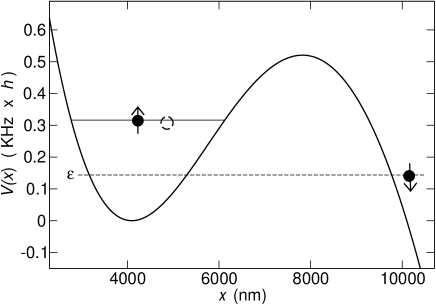
Figure 1: Confinement potential $V(x)$ vs $x$ as in Ref. Zuern2013, with $p=0.6338$ and $c_{B\left|\text{state}\right>}=1$. The frequency $\omega_{\text{WKB}}$ of the single bound state (solid thin line) computed through the WKB approximation is $\omega_{\text{WKB}}=$ 316.3 Hz $\times$ $2\pi$ (the trap bottom is the frequency zero). The tunneling energy for single-atom escape is $\varepsilon$. Note that for attractive interactions ($g<0$) one has $\varepsilon<\hbar\omega_{\text{WKB}}$ hence single-atom resonant tunneling is suppressed when $\varepsilon<0$. The circles with arrows schematize the atoms in the $\left|\uparrow\downarrow\right>$ final configuration.

In the combined optical and magnetic potential illustrated in Fig. 1, which is quasi one-dimensional due to the strong transverse confinement, two ⁶Li atoms behave as fermions of spin one-half and interact through an attractive tunable contact potential, $g\,\delta(x_{1}-x_{2})$, with $g<0$ (for the regime of strong repulsion see Ref. Wang2012b, ). A finite and smooth tunnel barrier allows atoms to escape from the trap into the unbound region at large positive values of $x$. The Hamiltonian is

$$H=-\frac{\hbar^{2}}{2m}\sum_{i=1}^{2}\left[\frac{d^{2}}{dx_{i}^{2}}+V(x_{i})\right]+g\delta(x_{1}-x_{2}),$$ (1)

with $m$ being the mass and $V(x)$ an effective potential. The exact functional form of $V(x)$ reproduces the setup of Ref. Zuern2013, (cf. Supplemental Material) with the optical trap depth parameter $p=0.6338$ and $c_{B\left|\text{state}\right>}=1$. The latter condition is equivalent to neglect the weak dependence of the atom magnetic moment (and hence the potential profile) on the atom spin.

The trap is approximately parabolic at low energy, the trap bottom being the energy zero. The bound trap eigenstates $\phi_{n}(x)$ are therefore eigenstates of the one-dimensional harmonic oscillator (HO), with energy $\varepsilon_{n}=\hbar\omega_{0}(n+1/2)$ and $n=0,1,2,\ldots$ The characteristic HO length is $\ell_{\text{HO}}=(\hbar/m\omega_{0})^{1/2}$. According to a WKB calculation, $V(x)$ supports a single bound state (cf. the solid thin line in Fig. 1), with $\omega_{\text{WKB}}=$ 316.3 Hz $\times$ $2\pi$.

Here only the $\left|\uparrow\downarrow\right>$ configuration of distinguishable fermions is considered, with the two atoms of opposite spin being paired in their ground state. Therefore, the orbital part of the $\left|\uparrow\downarrow\right>$ wave function is bosoniclike, $\psi_{\uparrow\downarrow}(x_{1},x_{2})=\psi_{\uparrow\downarrow}(x_{2},x_{1})$. The notation used throughout this Article is consistent with that of Ref. Rontani2012, .

III Decay law

In the experiment of Ref. Zuern2013, two  atoms are initially prepared in the ground state of the optical trap where the coupling constant $g$ is set by a Feshbach resonance tuning the magnetic offset field to a fixed value. A magnetic field gradient is then applied along $x$ for a given hold time $t$, whose effect is to add a linear term to the confinement potential. The net result, shown in Fig. 1, is to lower the potential barrier allowing for atoms to tunnel out of the trap. The measurement cycle ends by ramping the potential barrier back up and then counting the $N(t)$ survivor atoms left in the trap. Averaging over many measurement cycles provides the probabilities $P_{2}(t)$, $P_{1}(t)$, and $P_{0}(t)$ of finding respectively two, one, and zero atoms in the trap after the hold time $t$. From the conservation of probability one has $P_{2}(t)+P_{1}(t)+P_{0}(t)=1$ at all times, therefore only two quantities are independent, say $P_{2}(t)$ and $P_{1}(t)$. The measured mean atom number in the trap is $\left<N(t)\right>=2P_{2}(t)+P_{1}(t)$.

In this section we derive the decay law of $\left<N(t)\right>$ on the basis of simple rate equations, recalling the treatment of Ref. Zuern2013, for the sake of clarity. The decay is due to the combined effect of two qualitatively different tunneling processes, either the tunneling of a single atom or the correlated escape of two bound atoms at once. Both mechanisms may eventually empty the trap. We assume that the two tunneling rates, respectively $\gamma_{s}$ and $\gamma_{p}$ for single-atom and pair tunneling, may be computed independently.

At time $t$, $P_{2}(t)$ may decrease due to both single-atom or pair tunneling, so one has

$$\frac{dP_{2}(t)}{dt}=-\left(\gamma_{s}+\gamma_{p}\right)P_{2}(t).$$ (2)

Here the small probability that two consecutive single-atom tunneling events occur in the infinitesimal time interval $dt$ is neglected. Moreover, it is assumed that $\gamma_{s}$ and $\gamma_{p}$ are constant in time and add independently, as well as that the decay process is irreversible. The decay law is then simply

$$P_{2}(t)=e^{-\left(\gamma_{s}+\gamma_{p}\right)t}.$$ (3)

If $g=0$, there is no pair tunneling ($\gamma_{p}=0$) and $\gamma_{s}$ is twice the rate $\gamma_{s0}$ for the decay of a single atom in the trap, $\gamma_{s}=2\gamma_{s0}$ Kim2011b ; Rontani2012 ; Zuern2013 .

The variation in time of $P_{1}(t)$ is more complex,

$$\frac{dP_{1}(t)}{dt}=F_{\text{in}}(t)+F_{\text{out}}(t),$$ (4)

as $P_{1}(t)$ may either increase due to the one-atom decay of the state with two atoms, $F_{\text{in}}(t)=\gamma_{s}P_{2}(t)$, or decrease due to the decay of the one-atom state, $F_{\text{out}}(t)=-\gamma_{s0}P_{1}(t)$, so

$$\frac{dP_{1}(t)}{dt}=\gamma_{s}e^{-\left(\gamma_{s}+\gamma_{p}\right)t}-\gamma_{s0}P_{1}(t).$$ (5)

Solving Eq. (5) with the initial condition that there are two atoms in the trap [$P_{2}(0)=1$, $P_{1}(0)=P_{0}(0)=0$], the decay law is

$$P_{1}(t)=\frac{\gamma_{s}}{\gamma_{s}+\gamma_{p}-\gamma_{s0}}\left[e^{-\gamma_{s0}t}-e^{-\left(\gamma_{s}+\gamma_{p}\right)t}\right].$$ (6)

Therefore, the decay law for the mean particle number in the trap is:

$$\left<N(t)\right> = \left[2-\frac{\gamma_{s}}{\gamma_{s}+\gamma_{p}-\gamma_{s0}}\right]e^{-\left(\gamma_{s}+\gamma_{p}\right)t}$$ (7)

$$+ \frac{\gamma_{s}}{\gamma_{s}+\gamma_{p}-\gamma_{s0}}e^{-\gamma_{s0}t}.$$

In the noninteracting case one has

$$P_{2}(t)=e^{-2\gamma_{s0}t},$$ (8)

$$P_{1}(t)=2e^{-\gamma_{s0}t}\left[1-e^{-\gamma_{s0}t}\right],$$ (9)

$$P_{0}(t)=\left[1-e^{-\gamma_{s0}t}\right]^{2},$$ (10)

and it is easy to show that

$$P_{1}=\left<N\right>-\frac{1}{2}\left<N\right>^{2}$$ (11)

at all times $t$, which is the black dashed parabola of Fig. 3 in Zuern2013 . At finite $g$ it is not possible to work out a relation similar to (11) in closed form.

The next two sections explain the calculation of the tunneling rates $\gamma_{s}$, $\gamma_{s0}$, and $\gamma_{p}$ that enter the expressions (3) and (6) for $P_{2}(t)$ and $P_{1}(t)$, respectively.

IV Single-atom tunneling

This section focuses on the elementary tunneling event of a single atom transferred out of the trap. In the case there are initially two atoms in the trap, i.e., the tunneling transition is $N=2\rightarrow N=1$, the tunneling rate $\gamma_{s}$ is computed by means of the quasiparticle wave function theory developed in Ref. Rontani2012, . Such approach fully takes into account the interaction between the escaping atom and the companion left in the trap. The single-atom tunneling rate $\gamma_{s}$ is $1/\tau$ in the notation of Rontani2012 .

For attractive interactions, the relevant tunneling transition is the one between the initial trap ground state $\Psi_{0}(x_{1},x_{2})$ and the final noninteracting configuration $\Psi_{0,\varepsilon}(x_{1},x_{2})$, with one atom left in the lowest HO orbital $\phi_{0}(x)$ and the other one in the continuum state $\chi_{\varepsilon}(x)$ outside the trap (Fig. 1). If the total energy of the interacting state with two atoms in the trap is $W_{0}(g)$, from energy conservation it follows that the tunneling energy is $\varepsilon=W_{0}(g)-\varepsilon_{0}$. Here the two-atom energies and wave functions are computed in the harmonic approximation following the exact solution of Ref. Busch1998, .

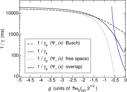
Figure 2: (color online). Inverse tunneling rates $1/\gamma$ vs coupling constant $g$ for $\omega_{0}=2\omega_{\text{WKB}}=632.6$ Hz $\times$ $2\pi$. $g$ is in units of $\hbar\omega_{0}2^{1/2}\ell_{\text{HO}}$.

When the tunneling energy is lower than the trap bottom, i.e., $\varepsilon<0$, the resonant tunneling process is forbidden. This is illustrated in Fig. 2, where $1/\gamma_{s}$ is plotted vs $g$ (blue [gray] line) for a trap with HO frequency $\omega_{0}=2\omega_{\text{WKB}}=632.6$ Hz $\times$ $2\pi$. The tunneling energy $\varepsilon$ and $\gamma_{s}$ decrease with increasing values of $\left|g\right|$, as the potential barrier faced by the escaping atom becomes higher and thicker. At $g\approx-0.65$ the energy $\varepsilon$ reaches the bottom of the trap where the channel of single-atom resonant tunneling closes.

In general, there may be final states other than $\Psi_{0,\varepsilon}$ allowed by energy conservation, like the $(n=1)(\varepsilon=W_{0}-\varepsilon_{1})$ configuration. However, the corresponding matrix elements may be neglected since wave function tails drop exponentially with energy in the barrier.

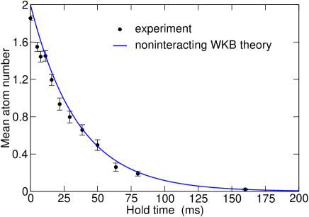
Figure 3: (color online). Mean atom number $\left<N(t)\right>$ vs hold time $t$. The points with their error bars are the measured values taken from Fig. 1 of Ref. Zuern2013, for $g=-0.01$ $\hbar\omega_{0}\ell_{\text{HO}}2^{1/2}$, with $\omega_{0}=$ 632.6 Hz $\times$ $2\pi$. The theoretical curve (continuous line) is a decaying exponential with time constant $1/\gamma_{s0}=35.24$ ms, as obtained from Eq. (12) with $\varepsilon_{0}=\hbar\omega_{\text{WKB}}=316.3$ Hz $\times$ $h$, with $\hbar\omega_{\text{WKB}}$ being the WKB energy of the bound state shown in Fig. 1.

In the case there is initially only one atom in the trap, the tunneling rate $\gamma_{s0}$ of the transition $N=1\rightarrow N=0$ is given by the WKB formula Zuern2012

$$\gamma_{s0}=\frac{\varepsilon_{0}}{2\pi}\exp{\left(-2\!\!\int_{x_{a}}^{x_{b}}\!\!\!k(x)dx\right)},$$ (12)

with $x_{a}<x_{b}$ being the classical turning points and $k(x)=[(2m/\hbar^{2})\left|\varepsilon_{0}-V(x)\right|]^{1/2}$. Here it is assumed that the atom in the trap occupies the lowest HO orbital $\phi_{0}(x)$.

In the case there are two noninteracting atoms one has $\gamma_{s}=2\gamma_{s0}$ and all decay laws assume a simple form, as shown in Sec. III. In particular, the mean atom number $\left<N(t)\right>$ is given by

$$\left<N(t)\right>=2e^{-\gamma_{s0}t},$$

as obtained from Eq. (7) with $\gamma_{p}=0$. Figure 3 compares such theoretical curve (continuous line), computed for $\varepsilon_{0}=\hbar\omega_{\text{WKB}}=316.3$ Hz $\times$ $h$, with the experimental data Zuern2013 (points) obtained for an almost negligible value of the coupling constant, $g=-0.01$ $\hbar\omega_{0}(2\hbar/m\omega_{0})^{1/2}$ ($\omega_{0}=2\omega_{\text{WKB}}=632.6$ Hz $\times$ $2\pi$), nicely showing the exponential decay whose time constant is given by the WKB prediction.

V Pair tunneling

In order to derive the pair tunneling rate $\gamma_{p}$, we rewrite the full Hamiltonian (1) in center-of-mass and relative-motion coordinates,

$$H=-\frac{\hbar^{2}}{m}\frac{d^{2}}{dx^{2}}+g\delta(x)-\frac{\hbar^{2}}{4m}\frac{d^{2}}{dX^{2}}+V(X+\frac{x}{2})+V(X-\frac{x}{2}),$$ (13)

with $X=(x_{1}+x_{2})/2$ and $x=x_{1}-x_{2}$. The time-independent Schrödinger equation reads

$$H\Psi(X,x)=W\Psi(X,x),$$ (14)

with $\Psi(X,x)$ being the two-atom ground state over the whole space (not to be confused with Bardeen’s solution $\Psi_{0}(x_{1},x_{2})$ of section IV, which is the ground state in the trap region and vanishes outside the potential barrier Rontani2012 ). In the following we are concerned with solutions of the eigenvalue problem (14) such that the two atoms form a bound state—a pair—both inside and outside the trap.

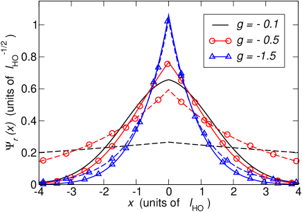
Figure 4: (color online). Relative-motion wave function $\Psi_{r}(x)$ vs $x$ for different values of $g$. The solid curves represent the ground states in a harmonic trap Busch1998 , whereas the dashed lines show the corresponding bound states in free space. The length unit is $\ell_{\text{HO}}=(\hbar/m\omega_{0})^{1/2}$ and $g$ is expressed in units of $\hbar\omega_{0}\ell_{\text{HO}}2^{1/2}$.

Close to the bottom of the trap the anharmonic terms of the potential are negligible, hence $V(X+x/2)+V(X-x/2)\approx m\omega_{0}^{2}X^{2}+m\omega_{0}^{2}x^{2}/4$ and the Hamiltonian (13) becomes separable with respect to coordinates $x$ and $X$, the wave function being $\Psi(X,x)=\Psi_{\text{CM}}(X)\Psi_{r}(x)$. In this region one may use the exact solution for $\Psi_{r}(x)$ Rontani2012 ; Busch1998 whereas $\Psi_{\text{CM}}(X)$ is just a Gaussian. We write the total energy as $W_{0}=E_{\text{trap}}+\varepsilon_{0}$, with only the relative-motion energy $E_{\text{trap}}$ depending on $g$. Figure 4 shows $\Psi_{r}(x)$ for different values of $g$ (solid lines). Here the energy unit is $\hbar\omega_{0}$, the length unit is $\ell_{\text{HO}}$, and $g$ is expressed in units of $\hbar\omega_{0}\ell_{\text{HO}}2^{1/2}$.

Even well outside the trap the wave function is decoupled, $\Psi(X,x)=\Psi_{\text{CM}}(X)\Psi_{r}(x)$. In this case $\Psi_{\text{CM}}(X)$ is a continuum state whereas $\Psi_{r}(x)$ is finite and normalizable, with wave function

$$\Psi_{r}(x)=\frac{\sqrt{-g}}{2^{1/4}}\exp{(g\left|x\right|/\sqrt{2})}$$ (15)

and energy $E_{\text{free}}=-g^{2}/2$ (here $\ell_{\text{HO}}=\hbar\omega_{0}=1$). The pair wave function $\Psi_{r}(x)$ is compared inside (solid lines) and outside (dashed lines) the trap in Fig. 4. For weak attraction ($g=-0.1$ and -0.5) the size of the pair outside the trap is much larger than inside the trap, the trap confinement potential squeezing $\Psi_{r}(x)$ and forcing it to have Gaussian tails. However, for stronger attraction ($g=-1.5$), the two wave functions overlap almost completely.

V.1 Effective Schrödinger equation from ansatz wave function

In the case the two atoms tunnel as a pair, a reasonable assumption is that the atoms form a bound state over the whole space. A possible ansatz wave function is then

$$\Psi(X,x)\approx\Psi_{\text{CM}}(X)\Psi_{r}(x)\quad\forall\,\,X,$$ (16)

with $\Psi_{r}(x)$ being the bound state wave function in the relative-motion frame obtained from Busch’s theory Busch1998 .

By multiplying both sides of Eq. (14) for $\Psi^{*}_{r}(x)$, using Eqs. (13), (16), and integrating over $x$, one obtains an effective Schrödinger equation for the center-of-mass motion:

$$-\frac{\hbar^{2}}{4m}\frac{d^{2}\Psi_{\text{CM}}(X)}{dX^{2}}+V_{\text{CM}}(X)\Psi_{\text{CM}}(X)=\varepsilon_{\text{CM}}\Psi_{\text{CM}}(X).$$ (17)

Here the effective potential $V_{\text{CM}}(X)$ is defined as

$$V_{\text{CM}}(X) = \int^{\infty}_{-\infty}\!\!\!dx\left|\Psi_{r}(x)\right|^{2}$$ (18)

$$\times \left[V(X+\frac{x}{2})+V(X-\frac{x}{2})-\frac{m}{4}\omega_{0}^{2}x^{2}\right],$$

and the center-of-mass energy $\varepsilon_{\text{CM}}$ is the total energy $W$ minus the relative-motion energy $E_{\text{trap}}$, $\varepsilon_{\text{CM}}=W-E_{\text{trap}}$. The energy $E_{\text{trap}}$ is the eigenvalue of the equation

$$\left[-\frac{\hbar^{2}}{m}\frac{d^{2}}{dx^{2}}+\frac{m}{4}\omega_{0}^{2}x^{2}+g\delta(x)\right]\Psi_{r}(x)=E_{\text{trap}}\Psi_{r}(x).$$ (19)

Equation (17) takes into account the internal degree of freedom of the two-atom bound state through the potential $V_{\text{CM}}(X)$, which is the original potential $V$ smeared by the relative-motion probability density $\left|\Psi_{r}(x)\right|^{2}$ appearing in (18).

To shed light on the structure of $V_{\text{CM}}(X)$, it is useful to consider two limiting cases. In case the potential profile is purely parabolic, $V(x)=m\omega_{0}^{2}x^{2}/2$, Eq. (18) simply reduces to $V_{\text{CM}}(X)=m\omega_{0}^{2}X^{2}$ and the ansatz wave function (16) is the exact result. The other exact limit is the case $g\rightarrow-\infty$. Then the pair binding energy goes to $-\infty$ and the spatial extension of $\Psi_{r}(x)$ becomes negligible, hence $\left|\Psi_{r}(x)\right|^{2}\approx\delta(x)$ and Eq. (18) becomes $V_{\text{CM}}(X)=2V(X)$. Equation (17) then takes the form

$$-\frac{\hbar^{2}}{4m}\frac{d^{2}\Psi_{\text{CM}}(X)}{dX^{2}}+2V(X)\Psi_{\text{CM}}(X)=\varepsilon_{\text{CM}}\Psi_{\text{CM}}(X),$$ (20)

which is the single-particle Schrödinger equation for a particle of coordinate $X$ and mass $2m$ seeing the potential 2$V(X)$.

In order to compute the pair tunneling rate $\gamma_{p}$, it suffices to note that the tunneling problem is reduced through (17) to that of a single particle of mass $2m$ escaping through the effective potential barrier defined by $V_{\text{CM}}(X)$. Then $\gamma_{p}$ may be computed trough the WKB formula

$$\gamma_{p}=\frac{\varepsilon_{\text{CM}}}{2\pi\hbar}\exp{\left(-2\!\!\int_{X_{a}}^{X_{b}}\!\!\!K(X)dX\right)}.$$ (21)

Here $X_{a}<X_{b}$ are the classical turning points for the effective potential $V_{\text{CM}}(X)$, $K(X)=[(4m/\hbar^{2})\left|\varepsilon_{\text{CM}}-V_{\text{CM}}(X)\right|]^{1/2}$, and the center-of-mass energy $\varepsilon_{\text{CM}}$ is the WKB bound level in the trap defined by $V_{\text{CM}}(X)$.

The dashed line in Fig. 2 shows $1/\gamma_{p}$ obtained for $\omega_{0}=2\omega_{\text{WKB}}=632.6$ Hz $\times$ $2\pi$. The inverse decay rate $1/\gamma_{p}$ increases with $\left|g\right|$, the smaller the pair size the lower the tunneling rate. For strong attraction $1/\gamma_{p}$ tends to the asymptotic exact limit of a point-like particle of mass $2m$. However, for $g\rightarrow 0$ the decay time $1/\gamma_{p}$ disturbingly tends to a finite value, whereas one would expect it to be suppressed as the atoms become unbound. Such difficulty is due to the approximate form (16) for $\Psi(X,x)$.

Alternatively, one may replace in the ansatz (16) the trap pair wave function with the bound state in free space [Eq. (15)]. The corresponding values obtained for $1/\gamma_{p}$ are shown by the dotted curve in Fig. 2. Reassuringly, for strong attraction the dotted and dashed curves overlap, as the pair wave functions tend to coincide. However, as $g\rightarrow 0$ the value of $1/\gamma_{p}$ becomes unphysically low, since the ansatz wave function now overestimates the pair size.

The missing piece of information in the ansatz (16) is the link between the pair wave function inside and outside the trap. Indeed, one expects $1/\gamma_{p}$ to interpolate between the upper and lower bounds represented respectively by the dashed and dotted curves in Fig. 2. An additional physical requirement is that $1/\gamma_{p}\rightarrow\infty$ as $g\rightarrow 0$. In the next subsection we propose a refined effective potential for the center-of-mass motion which complies with the required physical features.

V.2 Effective center-of-mass potential from time-dependent perturbation theory

As a preliminary step, we recall the result of time-dependent first-order perturbation theory Rontani2012 ; Bardeen1961 for the noninteracting single-atom tunneling rate $\gamma_{s0}$. Such rate is given by Fermi’s golden rule,

$$\gamma_{s0} = \frac{2\pi}{\hbar}\sum_{\varepsilon}\left|M_{0\varepsilon}\right|^{2}\delta(\varepsilon_{0}-\varepsilon)$$ (22)

$$= \frac{2\pi}{\hbar}\left|M_{0\varepsilon_{0}}\right|^{2}\varrho(\varepsilon_{0}),$$

with $\varrho(\varepsilon_{0})$ being the density of continuum states at energy $\varepsilon_{0}$ and

$$M_{0\varepsilon}=\int_{-\infty}^{\infty}\!\!\!dx\;\phi_{0}^{*}(x)\left[-\frac{\hbar^{2}}{2m}\frac{d^{2}}{dx^{2}}+V(x)-\varepsilon\right]\chi_{\varepsilon}(x).$$ (23)

For the following development, we remark that the practical evaluation of $\gamma_{s0}$ relies on the WKB formula (12). Therefore, we associate the matrix element (23) with the expression (12) for the decay of a particle of energy $\varepsilon$ and mass $m$ through the potential barrier $V(x)$.

Considering now the interacting case, the pair-tunneling matrix element ${\cal M}_{0f}$ between the initial state $\Psi_{0}(X,x)$ with two atoms in the trap and the final state $\Psi_{f}(X,x)$ with the pair outside the trap is a straightforward extension of (23):

$${\cal M}_{0f}=\int_{-\infty}^{\infty}\!\!\!dX\int_{-\infty}^{\infty}\!\!\!dx\;\Psi_{0}^{*}(X,x)\left[H-W_{f}\right]\Psi_{f}(X,x).$$ (24)

Both initial and final states are written as $\Psi(X,x)=\Psi_{\text{CM}}(X)\Psi_{r}(x)$, the relative and center-of-mass motions being decoupled. For the initial state, $\Psi_{0}(X,x)=\Psi^{0}_{\text{CM}}(X)\Psi^{0}_{r}(x)$, the relative-motion wave function $\Psi^{0}_{r}(x)$ is Busch’s solution with energy $E_{\text{trap}}(g)$ Busch1998 and $\Psi^{0}_{\text{CM}}(X)$ is the lowest HO state in the center-of-mass frame with energy $\varepsilon_{0}$, the total energy being $W_{0}=E_{\text{trap}}(g)+\varepsilon_{0}$. For the final state, $\Psi_{f}(X,x)=\Psi^{f}_{\text{CM}}(X)\Psi^{f}_{r}(x)$, the relative-motion wave function $\Psi^{f}_{r}(x)$ is the free-space wave function (15) with energy $E_{\text{free}}=-g^{2}/2$ and $\Psi_{\text{CM}}(X)$ is the continuum state with energy $\varepsilon_{\text{CM}}$, the total energy being $W_{f}=-g^{2}/2+\varepsilon_{\text{CM}}$.

The next step is to trace out the relative-motion degree of freedom in (24) by integrating over $x$. One obtains

$${\cal M}_{0f} = \int_{-\infty}^{\infty}\!\!\!dX\;\Psi^{0*}_{\text{CM}}(X)\bigg{[}-\frac{S\hbar^{2}}{4m}\frac{d^{2}}{dX^{2}}$$ (25)

$$+\;V_{\text{CM}}(X)-S\varepsilon_{\text{CM}}\bigg{]}\Psi^{f}_{\text{CM}}(X),$$

with $S$ being the overlap integral between relative-motion wave functions,

$$S=\int_{-\infty}^{\infty}\!\!\!dx\;\Psi^{0*}_{r}(x)\,\Psi^{f}_{r}(x),$$ (26)

and $V_{\text{CM}}(X)$ being the effective potential for center-of-mass motion,

$$V_{\text{CM}}(X) = \int_{-\infty}^{\infty}\!\!\!dx\;\Psi^{0*}_{r}(x)\,\Psi^{f}_{r}(x)$$ (27)

$$\times \left[V(X+x/2)+V(X-x/2)\right].$$

By inspection we see that the formula (25) is the matrix element for the decay of a particle of mass $2m/S$ and energy $S\varepsilon_{\text{CM}}$ through the potential barrier $V_{\text{CM}}(X)$. The latter effective potential is smeared by the overlap density $\Psi^{0*}_{r}(x)\,\Psi^{f}_{r}(x)$ instead of the probability density $\left|\Psi_{r}(x)\right|^{2}$ that appears in (18).

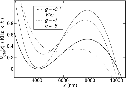
Figure 5: Effective confinement potential for the center-of-mass motion $V_{\text{CM}}(x)$ vs $x$, as defined in Eq. (27), for a few values of the coupling constant $g$. Here the HO frequency is $\omega_{0}=$ 250 Hz $\times$ $2\pi$ (the trap bottom is the frequency zero). The coupling constant $g$ is expressed in units of $\hbar\omega_{0}\ell_{\text{HO}}2^{1/2}$, with $\ell_{\text{HO}}=(\hbar/m\omega_{0})^{1/2}$. The thick solid line is the original single-particle bare potential $V(x)$.

The potential barrier induced by $V_{\text{CM}}(X)$ depends on the coupling constant $g$, as shown in Fig. 5. For strong attraction, $g\rightarrow-\infty$, the overlap density $\Psi^{0*}_{r}(x)\,\Psi^{f}_{r}(x)$ tends to the probability density $\left|\Psi_{r}(x)\right|^{2}$ and $S\rightarrow 1$, hence one recovers the results of subsection V.1. In fact, the effective particle of mass $2m/S\rightarrow 2m$ and energy $S\varepsilon_{\text{CM}}\rightarrow\varepsilon_{\text{CM}}$ sees a potential barrier $V_{\text{CM}}(x)\rightarrow 2V(x)$ (compare thin and thick solid lines in Fig. 5). However, for $g\rightarrow 0$ the effective one-particle problem strongly deviates from that of subsection V.1, as now the particle acquires infinite mass since $S\rightarrow 0$.

The above discussion shows that $\gamma_{p}$ may be evaluated by means of the WKB formula (21) using the expression (27) for $V_{\text{CM}}(X)$ and replacing $2m$ with $2m/S$ as well as $\varepsilon_{\text{CM}}$ with $S\varepsilon_{\text{CM}}$. The result for $\omega_{0}=2\omega_{\text{WKB}}=632.6$ Hz $\times$ $2\pi$ is shown in Fig. 2 (black solid line). One recovers the previous results of subsection V.1 for $g\rightarrow-\infty$, as all black curves tend to the same line asymptotically.

The small discrepancy between solid and dashed / dotted lines for large values of $\left|g\right|$ is due to the different method to determine $\varepsilon_{\text{CM}}$. In fact, for the black solid curve $\varepsilon_{\text{CM}}$ is fixed by energy conservation, $\varepsilon_{\text{CM}}=\varepsilon_{0}+E_{\text{trap}}(g)+g^{2}/2$, whereas for the dashed and dotted curves $\varepsilon_{\text{CM}}$ is the WKB energy of the bound state in the effective potential. Nevertheless, in the limit $g\rightarrow-\infty$ one has $\varepsilon_{\text{CM}}\rightarrow\varepsilon_{0}$ and the curves are expected to merge.

For moderate attraction the behavior of the black solid curve in Fig. 2 strongly departs from those of the dashed and dotted curves. In fact, $1/\gamma_{p}$ interpolates between dashed and dotted curves, first showing a minimum as $\left|g\right|$ is decreased and then going to $+\infty$ as $g\rightarrow 0$. Such trend complies with the physical expectation that correlated tunneling is forbidden in the absence of interaction and that it is favored by the extension of the pair, the larger the pair size the fatter the wave function tail in the barrier.

V.3 Discussion

In principle pair tunneling may be investigated numerically simulating the full quantum mechanical time evolution of two atoms that are allowed to escape from the trap, as it was done for repulsive interactions in Refs. Lode2009, ; Kim2011b, ; Lode2012, ; Hunn2013, . However, the present case of attractive interactions raises a computational issue on the accuracy of the interacting wave function. In fact, the two-body wave function in the relative frame collapses in space with increasing attraction Busch1998 . Hence, a larger basis set is neeeded in typical variational methods Rontani2006 ; Lode2009 ; Kim2011b ; Lode2012 ; Hunn2013 to provide a certain numerical accuracy, which implies either a higher-energy cutoff or a higher resolution in real space, as we discuss at length elsewhere DAmico2013 .

Besides, it is difficult to treat numerically realistic tunnel barriers that are typically shallow, as the one shown in Fig. 1. As a matter of fact, previous numerical approaches for repulsive interactions Lode2009 ; Kim2011b ; Lode2012 ; Hunn2013 considered only idealized functional forms of potential profiles. The approximate theory presented in this work is fit to any potential profile and interaction strength.

VI Comparison with the Heidelberg experiment

Since the tunneling rates in the experiment Zuern2013 are the outcome of a complex fitting procedure involving different measurements, for the sake of clarity we consider a single observable, that is the decay time of $P_{2}(t)$. Such quantity is easily obtained in both theory and experiment. In the former it is simply $1/(\gamma_{s}+\gamma_{p})$ according to Eq. (3), whereas in the latter it is a straightforward exponential fitting to measured data, as shown in Fig. 3 for the noninteracting case.

Figure 6 compares the measured and predicted values of $1/(\gamma_{s}+\gamma_{p})$ as a function of the coupling constant $g$. We remark that in our theory the fitting parameter is the HO frequency $\omega_{0}$. This fixes the interaction energy for a certain value of $g$ Busch1998 , whereas in Ref. Zuern2013, the interaction energy is the output of the fitting procedure, the fitting parameters being the tunneling rates. Besides, the determination of $\omega_{0}$ is a non-trivial experimental task, being specific to the type of spectroscopy Zuern2013 ; Wenz2013 .

The natural choice for the free parameter $\omega_{0}$ would be $\omega_{0}=2\omega_{\text{WKB}}$, as one may regards $\hbar\omega_{\text{WKB}}$ as the zero-point energy of the HO. This was also the value chosen to compute the tunneling rates in the interacting case shown in Fig. 2. However, the predicted values of the tunneling rates turn out to be systematically small with respect to the measured values Zuern2013 .

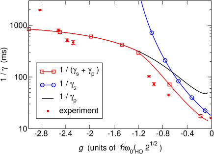
Figure 6: (color online). Inverse tunneling rates $1/\gamma$ vs coupling constant $g$ for $\omega_{0}=250$ Hz $\times$ $2\pi$. $g$ is in units of $\hbar\omega_{0}(2\hbar/m\omega_{0})^{1/2}$. The points with their error bars are the measured values of $1/(\gamma_{s}+\gamma_{p})$, extracted from Table III of Ref. Zuern2013, (column $\gamma_{2,\text{fit}}$) except for the rightmost point that is taken from our Fig. 3. The red [light gray] curve is the theoretical estimate, as explained in the main text.

The chosen value of $\omega_{0}$ in Fig. 6 is $\omega_{0}=$ 250 Hz $\times$ $2\pi$, with $\varepsilon_{0}=\hbar\omega_{\text{WKB}}$ and $E_{\text{trap}}(g)=\hbar\omega_{0}\left[\tilde{E}_{\text{trap}}(g)-1/2\right]+\hbar\omega_{\text{WKB}}$, $\tilde{E}_{\text{trap}}(g)$ being the relative-motion energy in units of $\hbar\omega_{0}$ according to Ref. Busch1998, . The blue [gray] curve is the quasiparticle prediction for $1/\gamma_{s}$, which deviates only slightly (within 10%) from the noninteracting WKB value $1/(2\gamma_{s0})$. The black curve is $1/\gamma_{p}$ calculated following the method outlined in subsection V.2. The points are the measured values of $1/(\gamma_{s}+\gamma_{p})$ with their error bars, taken from Table III of Ref. Zuern2013, (column $\gamma_{2,\text{fit}}$) except for the rightmost point that is taken from our Fig. 3. Note that the values of $g$ were rescaled due to the different HO reference frequency.

The theoretical value of $1/(\gamma_{s}+\gamma_{p})$ (solid red [light gray] curve) fairly compares with the measured points, exhibiting the same qualitative trend. We note that at small values of $\left|g\right|$ the measured values of $1/(\gamma_{s}+\gamma_{p})$ are smaller than the theoretical ones, whereas at large $\left|g\right|$ the opposite holds. This suggests that the effective frequency $\omega_{0}$ increases with $\left|g\right|$, since the smaller $\omega_{0}$ the smaller $1/(\gamma_{s}+\gamma_{p})$. Such behavior appears reasonable as the HO frequency obtained by expanding $V(x)$ around the trap bottom is larger than $2\omega_{\text{WKB}}$. Therefore, one expects larger anharmonic effects at higher energies, i.e., at smaller values of $\left|g\right|$. This confirms a posteriori that neglecting the effects of the anharmonic terms of the potential on the two-body wave function is a reasonable approximation.

All data measured in Ref. Zuern2013, were explained assuming no pair tunneling, $\gamma_{p}=0$. However, the error of the measurements performed in the regime of strong attraction was too large to exclude unambiguously the occurrence of pair tunneling. Figure 6 shows that the channel associated to usual single-atom tunneling (blue [gray] solid line) closes already at moderate values of $g\sim 1$. This prediction paves the way to future experiments in the regime of moderate attraction, where only pair tunneling is expected to survive.

VII Conclusions

In this Article we have developed a theory of the pair tunneling of two fermions out of a trap that is based on simple and physically transparent formulae. We predict that the observation of pair tunneling is within reach of present experiments with ⁶Li atoms. Intriguingly, it was recently showed Rontani2009c ; Zuern2013 that pairing emerges already with very few atoms in tight low-dimensional traps. Therefore, pair tunneling may provide an important spectroscopic tool to address pairing in many-body states.

- (1) P. G. de Gennes, Superconductivity of metals and alloys (Westview Press, Boulder (Colorado), 1999)
- (2) A. B. Migdal, Zh. Eksp. i Teor. Fiz. Pisma 37, 249 (1959), [Sov. Phys.–JETP 10, 176 (1960)]
- (3) A. Bohr and B. R. Mottelson, Nuclear structure — Vol. I and II (World Scientific, Singapore, 1998)
- (4) V. L. Ginzburg and D. A. Kirzhnits, Zh. Eksp. i Teor. Fiz. Pisma 47, 2006 (1965), [Sov. Phys.–JETP 20, 1346 (1965)]
- (5) D. Pines, G. Baym, and C. Pethick, Nature 224, 673 (1969)
- (6) A. J. Leggett, Quantum liquids, 1st ed. (Oxford University Press, Oxford, 2006)
- (7) M. Rontani and L. J. Sham, “Novel superfluids volume 2,” (Oxford University Press, Oxford, UK, 2013) preprint at arXiv:1301.1726
- (8) J. Bardeen, L. N. Cooper, and J. R. Schrieffer, Phys. Rev. 108, 1175 (1957)
- (9) A. Barone and G. Paterno, Physics and applications of the Josephson effect (Wiley, New York, 1982)
- (10) A. F. Andreev, Zh. Eksp. i Teor. Fiz. 46, 1823 (1964), [Sov. Phys.–JETP 19, 1228 (1964)]
- (11) F. Serwane, G. Zürn, T. Lompe, T. B. Ottenstein, A. N. Wenz, and S. Jochim, Science 332, 336 (2011)
- (12) G. Zürn, F. Serwane, T. Lompe, A. N. Wenz, M. G. Ries, J. E. Bohn, and S. Jochim, Phys. Rev. Lett. 108, 075303 (2012)
- (13) G. Zürn, A. N. Wenz, S. Murmann, T. Lompe, and S. Jochim(2013), arXiv:1307.5153v1
- (14) C. Chin, R. Grimm, P. Julienne, and E. Tiesinga, Rev. Mod. Phys. 82, 1225 (2010)
- (15) C. A. Regal, C. Ticknor, J. L. Bohn, and D. S. Jin, Nature (London) 424, 47 (2003)
- (16) M. Bartenstein, A. Altmeyer, S. Riedl, S. Jochim, C. Chin, J. H. Denschlag, and R. Grimm, Phys. Rev. Lett. 92, 120401 (2004)
- (17) M. W. Zwierlein, J. R. Abo-Shaeer, A. Schirotzek, C. H. Schunck, and W. Ketterle, Nature (London) 435, 1047 (2005)
- (18) S. Giorgini, L. P. Pitaevskii, and S. Stringari, Rev. Mod. Phys. 80, 1215 (2008)
- (19) M. Rontani, Phys. Rev. Lett. 108, 115302 (2012)
- (20) A. M. Dudarev, M. G. Raizen, and Q. Niu, Phys. Rev. Lett. 98, 063001 (2007)
- (21) P. Cheinet, S. Trotzky, M. Feld, U. Schnorrberger, M. Moreno-Cardoner, S. Fölling, and I. Bloch, Phys. Rev. Lett. 101, 090404 (2008)
- (22) A. del Campo, F. Delgado, G. García-Calderón, J. G. Muga, and M. G. Raizen, Phys. Rev. A 74, 013605 (2006)
- (23) A. del Campo, Phys. Rev. A 84, 012113 (2011)
- (24) G. García-Calderón and L. G. Mendoza-Luna, Phys. Rev. A 84, 032106 (2011)
- (25) D. Sokolovski, M. Pons, and T. Kamalov, Phys. Rev. A 86, 022110 (2012)
- (26) S. Longhi and G. D. Valle, Phys. Rev. A 86, 012112 (2012)
- (27) M. Pons, D. Sokolovski, and A. del Campo, Phys. Rev. A 85, 022107 (2012)
- (28) O. Georgiou, G. Glicorić, A. Lazarides, D. F. M. Oliveira, J. D. Bodyfelt, and A. Goussev, Europhys. Lett. 100, 20005 (2012)
- (29) M. Girardeau, J. Math. Phys. (N.Y.) 1, 516 (1960)
- (30) T. Cheon and T. Shigehara, Phys. Rev. Lett. 82, 2536 (1999)
- (31) S. Zöllner, H.-D. Meyer, and P. Schmelcher, Phys. Rev. Lett. 100, 040401 (2008)
- (32) A. I. Streltsov, K. Sakmann, O. E. Alon, and L. S. Cederbaum, Phys. Rev. A 83, 043604 (2011)
- (33) B. Chatterjee, I. Brouzos, L. Cao, and P. Schmelcher, Phys. Rev. A 85, 013611 (2012)
- (34) S. Hunn, K. Zimmermann, M. Hiller, and A. Buchleitner, Phys. Rev. A 87, 043626 (2013)
- (35) P. O. Bugnion and G. J. Conduit, Phys. Rev. A 88, 013601 (2013)
- (36) A. U. J. Lode, A. I. Streltsov, O. E. Alon, H.-D. Meyer, and L. S. Cederbaum, J. Phys. B 42, 044018 (2009)
- (37) S. Kim and J. Brand, J. Phys. B: At. Mol. Opt. Phys. 44, 195301 (2011)
- (38) A. U. J. Lode, A. I. Streltsov, K. Sakmann, O. E. Alon, and L. S. Cederbaum, Proc. Natl. Acad. Sci. USA 109, 13521 (2012)
- (39) J. Bardeen, Phys. Rev. Lett. 6, 57 (1961)
- (40) M. D. Girardeau and G. E. Astrakharchik, Phys. Rev. A 81, 061601(R) (2010)
- (41) M. D. Girardeau, Phys. Rev. A 82, 011607(R) (2010)
- (42) P. O. Bugnion and G. J. Conduit, Phys. Rev. A 87, 060502(R) (2013)
- (43) T. Taniguchi and S. I. Sawada, Phys. Rev. E 83, 026208 (2011)
- (44) M. Razavy, Quantum theory of tunneling (World Scientific, Singapore, 2003)
- (45) S. R. Wilkinson, C. F. Bharucha, M. C. Fisher, K. W. Madison, P. R. Morrow, Q. Niu, B. Sundaram, and M. G. Raizen, Nature (London) 387, 575 (1997)
- (46) C. Rothe, S. I. Hintschich, and A. P. Monkman, Phys. Rev. Lett. 96, 163601 (2006)
- (47) J.-J. Wang, W. Li, S. Chen, G. Xianlong, M. Rontani, and M. Polini, Phys. Rev. B 86, 075110 (2012)
- (48) T. Busch, B. Englert, K. Rza̧żewski, and M. Wilkens, Found. Phys. 28, 549 (1998)
- (49) M. Rontani, C. Cavazzoni, D. Bellucci, and G. Goldoni, J. Chem. Phys. 124, 124102 (2006)
- (50) P. D’Amico and M. Rontani(2013), arXiv:1310.3829
- (51) A. N. Wenz, G. Zürn, S. Murmann, I. Brouzos, T. Lompe, and S. Jochim(2013), arXiv:1307.3443v1
- (52) M. Rontani, J. R. Armstrong, Y. Yu, S. Åberg, and S. M. Reimann, Phys. Rev. Lett. 102, 060401 (2009)