Approximate Cone Factorizations
and Lifts of Polytopes

Abstract.

In this paper we show how to construct inner and outer convex approximations of a polytope from an approximate cone factorization of its slack matrix. This provides a robust generalization of the famous result of Yannakakis that polyhedral lifts of a polytope are controlled by (exact) nonnegative factorizations of its slack matrix. Our approximations behave well under polarity and have efficient representations using second order cones. We establish a direct relationship between the quality of the factorization and the quality of the approximations, and our results extend to generalized slack matrices that arise from a polytope contained in a polyhedron.

1. Introduction

A well-known idea in optimization to represent a complicated convex set $C\subset\mathbb{R}^{n}$ is to describe it as the linear image of a simpler convex set in a higher dimensional space, called a lift or extended formulation of $C$ . The standard way to express such a lift is as an affine slice of some closed convex cone $K$, called a $K$-lift of $C$, and the usual examples of $K$ are nonnegative orthants $\mathbb{R}^{m}_{+}$ and the cones of real symmetric positive semidefinite matrices $\mathcal{S}_{+}^{m}$. More precisely, $C$ has a $K$-lift, where $K\subset\mathbb{R}^{m}$, if there exists an affine subspace $L\subset\mathbb{R}^{m}$ and a linear map $\pi\,:\,\mathbb{R}^{m}\rightarrow\mathbb{R}^{n}$ such that $C=\pi(K\cap L)$.

Given a nonnegative matrix $M\in\mathbb{R}^{p\times q}_{+}$ and a closed convex cone $K\subset\mathbb{R}^{m}$ with dual cone $K^{\ast}\subset(\mathbb{R}^{m})^{\ast}$, a $K$-factorization of $M$ is a collection of elements $a_{1},\ldots,a_{p}\in K^{\ast}$ and $b_{1},\ldots,b_{q}\in K$ such that $M_{ij}=\langle a_{i},b_{j}\rangle$ for all $i,j$. In particular, a $\mathbb{R}^{m}_{+}$-factorization of $M$, also called a nonnegative factorization of $M$ of size $m$, is typically expressed as $M=A^{T}B$ where $A$ has columns $a_{1},\ldots,a_{p}\in(\mathbb{R}^{m})^{\ast}_{+}$ and $B$ has columns $b_{1},\ldots,b_{q}\in\mathbb{R}^{m}_{+}$. In [20], Yannakakis laid the foundations of polyhedral lifts of polytopes by showing the following.

Theorem 1.1.

[20] A polytope $P\subset\mathbb{R}^{n}$ has a $\mathbb{R}^{m}_{+}$-lift if and only if the slack matrix of $P$ has a $\mathbb{R}^{m}_{+}$-factorization.

This theorem was extended in [8] from $\mathbb{R}^{m}_{+}$-lifts of polytopes to $K$-lifts of convex sets $C\subset\mathbb{R}^{n}$, where $K$ is any closed convex cone, via $K$-factorizations of the slack operator of $C$.

The above results rely on exact cone factorizations of the slack matrix or operator of the given convex set, and do not offer any suggestions for constructing lifts of the set in the absence of exact factorizations. In many cases, one only has access to approximate factorizations of the slack matrix, typically via numerical algorithms. In this paper we show how to take an approximate $K$-factorization of the slack matrix of a polytope and construct from it an inner and outer convex approximation of the polytope. Our approximations behave well under polarity and admit efficient representations via second order cones. Further, we show that the quality of our approximations can be bounded by the error in the corresponding approximate factorization of the slack matrix.

Let $P:=\{x\in\mathbb{R}^{n}\,:\,H^{T}x\leq{\mathbbm{1}}\}$ be a full-dimensional polytope in $\mathbb{R}^{n}$ with the origin in its interior, and vertices $p_{1},\ldots,p_{v}$. We may assume without loss of generality that each inequality $\langle h_{i},x\rangle\leq 1$ in $H^{T}x\leq{\mathbbm{1}}$ defines a facet of $P$. If $H$ has size $n\times f$, then the slack matrix of $P$ is the $f\times v$ nonnegative matrix $S$ whose $(i,j)$-entry is $S_{ij}=1-\langle h_{i},p_{j}\rangle$, the slack of the $j$th vertex in the $i$th inequality of $P$. Given an $\mathbb{R}^{m}_{+}$-factorization of $S$, i.e., two nonnegative matrices $A$ and $B$ such that $S=A^{T}B$, an $\mathbb{R}^{m}_{+}$-lift of $P$ is obtained as

$$P=\left\{x\in\mathbb{R}^{n}\,:\,\exists y\in\mathbb{R}^{m}_{+}\textup{ s.t. }H^{T}x+A^{T}y={\mathbbm{1}}\right\}.$$

Notice that this lift is highly non-robust, and small perturbations of $A$ make the right hand side empty, since the linear system $H^{T}x+A^{T}y={\mathbbm{1}}$ is in general highly overdetermined. The same sensitivity holds for all $K$-factorizations and lifts. Hence, it becomes important to have a more robust, yet still efficient, way of expressing $P$ (at least approximately) from approximate $K$-factorizations of $S$. Also, the quality of the approximations of $P$ and their lifts must reflect the quality of the factorization, and specialize to the Yannakakis setting when the factorization is exact. The results in this paper carry out this program and contain several examples, special cases, and connections to the recent literature.

1.1. Organization of the paper

In Section 2 we establish how an approximate $K$-factorization of the slack matrix of a polytope $P\subset\mathbb{R}^{n}$ yields a pair of inner and outer convex approximations of $P$ which we denote as $\textup{Inn}_{P}(A)$ and $\textup{Out}_{P}(B)$ where $A$ and $B$ are the two “factors” in the approximate $K$-factorization. These convex sets arise naturally from two simple inner and outer second order cone approximations of the nonnegative orthant. While the outer approximation is always closed, the inner approximation maybe open if $K$ is an arbitrary cone. However, we show that if the polar of $K$ is “nice” [13], then the inner approximation will be closed. All cones of interest to us in this paper such as nonnegative orthants, positive semidefinite cones, and second order cones are nice. Therefore, we will assume that our approximations are closed after a discussion of their closedness.

We prove that our approximations behave well under polarity, in the sense that

$$\textup{Out}_{P^{\circ}}(A)=(\textup{Inn}_{P}(A))^{\circ}\quad\textup{ and }\quad\textup{Inn}_{P^{\circ}}(B)=(\textup{Out}_{P}(B))^{\circ}$$

where $P^{\circ}$ is the polar polytope of $P$. Given $P\subset\mathbb{R}^{n}$ and $K\subset\mathbb{R}^{m}$, our approximations admit efficient representations via slices and projections of $K\times\textup{SOC}_{n+m+2}$ where $\textup{SOC}_{k}$ is a second order cone of dimension $k$. We show that an $\varepsilon$-error in the $K$-factorization makes $\frac{1}{1+\varepsilon}P\subseteq\textup{Inn}_{P}(A)$ and $\textup{Out}_{P}(B)\subseteq(1+\varepsilon)P$, thus establishing a simple link between the error in the factorization and the gap between $P$ and its approximations. In the presence of an exact $K$-factorization of the slack matrix, our results specialize to the Yannakakis setting.

In Section 3 we discuss two connections between our approximations and well-known constructions in the literature. In the first part we show that our inner approximation, $\textup{Inn}_{P}(A)$, always contains the Dikin ellipsoid used in interior point methods. Next we examine the closest rank one approximation of the slack matrix obtained via a singular value decomposition and the approximations of the polytope produced by it.

In Section 4 we extend our results to the case of generalized slack matrices that arise from a polytope contained in a polyhedron. We also show how an approximation of $P$ with a $K$-lift produces an approximate $K$-factorization of the slack matrix of $P$. It was shown in [5] that the max clique problem does not admit polyhedral approximations with small polyhedral lifts. We show that this negative result continues to hold even for the larger class of convex approximations considered in this paper.

2. From approximate factorizations to approximate lifts

In this section we show how to construct inner and outer approximations of a polytope $P$ from approximate $K$-factorizations of the slack matrix of $P$, and establish the basic properties of these approximations.

2.1. $K$-factorizations and linear maps

Let $P=\{x\in\mathbb{R}^{n}\,:\,H^{T}x\leq{\mathbbm{1}}\}$ be a full-dimensional polytope with the origin in its interior. The vertices of the polytope are $p_{1},\ldots,p_{v}$, and each inequality $\langle h_{i},x\rangle\leq 1$ for $i=1,\ldots,f$ in $H^{T}x\leq{\mathbbm{1}}$ defines a facet of $P$. The slack matrix $S$ of $P$ is the $f\times v$ matrix with entries $S_{ij}=1-\langle h_{i},p_{j}\rangle$. In matrix form, letting $H=[h_{1}\ldots h_{f}]$ and $V=[p_{1}\ldots p_{v}]$, we have the expression $S={\mathbbm{1}}_{f\times v}-H^{T}V$. We assume $K\subset\mathbb{R}^{m}$ is a closed convex cone, with dual cone $K^{\ast}=\{y\in(\mathbb{R}^{m})^{\ast}\,:\,\langle y,x\rangle\geq 0\quad\forall x\in K\}$.

Definition 2.1.

([8]) A $K$-factorization of the slack matrix $S$ of the polytope $P$ is given by $a_{1},\ldots,a_{f}\in K^{\ast}$, $b_{1},\ldots,b_{v}\in K$ such that $1-\langle h_{i},p_{j}\rangle=\langle a_{i},b_{j}\rangle$ for $i=1,\ldots,f$ and $j=1,\ldots,v$. In matrix form, this is the factorization

$$S={\mathbbm{1}}_{f\times v}-H^{T}V=A^{T}B$$

where $A=[a_{1}\ldots a_{f}]$ and $B=[b_{1}\ldots b_{v}]$.

It is convenient to interpret a $K$-factorization as a composition of linear maps as follows. Consider $B$ as a linear map from $\mathbb{R}^{v}\rightarrow\mathbb{R}^{m}$, verifying $B(\mathbb{R}^{v}_{+})\subseteq K$. Similarly, think of $A$ as a linear map from $(\mathbb{R}^{f})^{\ast}\rightarrow(\mathbb{R}^{m})^{\ast}$ verifying $A((\mathbb{R}^{f})^{\ast}_{+})\subseteq K^{\ast}$. Then, for the adjoint operators, $B^{\ast}(K^{\ast})\subseteq(\mathbb{R}^{v})^{\ast}_{+}$ and $A^{\ast}(K)\subseteq\mathbb{R}^{f}_{+}$. Furthermore, we can think of the slack matrix $S$ as an affine map from $\mathbb{R}^{v}$ to $\mathbb{R}^{f}$, and the matrix factorization in Definition 2.1 suggests to define the slack operator, $S:\mathbb{R}^{v}\rightarrow\mathbb{R}^{f}$, as $S(x)=({\mathbbm{1}}_{f\times v}-H^{\ast}\circ V)(x)$, where $V:\mathbb{R}^{v}\rightarrow\mathbb{R}^{n}$ and $H:(\mathbb{R}^{f})^{\ast}\rightarrow(\mathbb{R}^{n})^{\ast}$.

We define a nonnegative $K$-map from $\mathbb{R}^{v}\rightarrow\mathbb{R}^{m}$ (where $K\subseteq\mathbb{R}^{m}$) to be any linear map $F$ such that $F(\mathbb{R}_{+}^{v})\subseteq K$. In other words, a nonnegative $K$-map from $\mathbb{R}^{v}\rightarrow\mathbb{R}^{m}$ is the linear map induced by an assignment of an element $b_{i}\in K$ to each unit vector $e_{i}\in\mathbb{R}^{v}_{+}$. In this language, a $K$-factorization of $S$ corresponds to a nonnegative $K^{\ast}$-map $A\,:\,(\mathbb{R}^{f})^{\ast}\rightarrow(\mathbb{R}^{m})^{\ast}$ and a nonnegative $K$-map $B\,:\,\mathbb{R}^{v}\rightarrow\mathbb{R}^{m}$ such that $S(x)=(A^{\ast}\circ B)(x)$ for all $x\in\mathbb{R}^{v}$. As a consequence, we have the correspondence $a_{i}:=A(e_{i}^{*})$ for $i=1,\ldots,f$ and $b_{j}:=B(e_{j})$ for $j=1,\ldots,v$.

2.2. Approximations of the nonnegative orthant

In this section we introduce two canonical second order cone approximations to the nonnegative orthant, which will play a crucial role in our developments. In what follows, $\|\cdot\|$ will always denote the standard Euclidean norm in $\mathbb{R}^{n}$, i.e., $\|x\|=(\sum_{i=1}^{n}x_{i}^{2})^{\frac{1}{2}}$.

Definition 2.2.

Let $\mathcal{O}_{in}^{n}$, $\mathcal{O}_{out}^{n}$ be the cones

$$\mathcal{O}_{in}^{n} :=\{x\in\mathbb{R}^{n}\,:\,\sqrt{n-1}\cdot\|x\|\leq\mathbbm{1}^{T}x\}$$

$$\mathcal{O}_{out}^{n} :=\{x\in\mathbb{R}^{n}\,:\,\|x\|\leq\mathbbm{1}^{T}x\}.$$

If the dimension $n$ is unimportant or obvious from the context, we may drop the superscript and just refer to them as $\mathcal{O}_{in}$ and $\mathcal{O}_{out}$.

As the following lemma shows, the cones $\mathcal{O}_{in}$ and $\mathcal{O}_{out}$ provide inner and outer approximations of the nonnegative orthant, which are dual to each other and can be described using second-order cone programming ([1, 10]).

Lemma 2.3.

The cones $\mathcal{O}_{in}$ and $\mathcal{O}_{out}$ are proper cones (i.e., convex, closed, pointed and solid) in $\mathbb{R}^{n}$ that satisfy

$$\mathcal{O}_{in}\subseteq\mathbb{R}^{n}_{+}\subseteq\mathcal{O}_{out},$$

and furthermore, $\mathcal{O}_{in}^{*}=\mathcal{O}_{out}$, and $\mathcal{O}_{out}^{*}=\mathcal{O}_{in}$.

The cones $\mathcal{O}_{in}$ and $\mathcal{O}_{out}$ are in fact the “best” second-order cone approximations of the nonnegative orthant, in the sense that they are the largest/smallest permutation-invariant cones with these containment properties; see also Remark 2.5. Lemma 2.3 is a direct consequence of the following more general result about (scaled) second-order cones:

Lemma 2.4.

Given $\omega\in\mathbb{R}^{n}$ with $\|\omega\|=1$ and $0<a<1$, consider the set

$$K_{a}:=\{x\in\mathbb{R}^{n}\,:\,a\|x\|\leq\omega^{T}x\}.$$

Then, $K_{a}$ is a proper cone, and $K_{a}^{*}=K_{b}$, where $b$ satisfies $a^{2}+b^{2}=1$, $b>0$.

Proof:   The set $K_{a}$ is clearly invariant under nonnegative scalings, so it is a cone. Closedness and convexity of $K_{a}$ follow directly from the fact that (for $a\geq 0$) the function $x\mapsto a\|x\|-\omega^{T}x$ is convex. The vector $\omega$ is an interior point (since $a\|\omega\|-\omega^{T}\omega=a-1<0$), and thus $K_{a}$ is solid. For pointedness, notice that if both $x$ and $-x$ are in $K_{a}$, then adding the corresponding inequalities we obtain $2a\|x\|\leq 0$, and thus (since $a>0$) it follows that $x=0$.

The duality statement $K_{a}^{*}=K_{b}$ is perhaps geometrically obvious, since $K_{a}$ and $K_{b}$ are spherical cones with “center” $\omega$ and half-angles $\theta_{a}$ and $\theta_{b}$, respectively, with $\cos\theta_{a}=a$, $\cos\theta_{b}=b$, and $\theta_{a}+\theta_{b}=\pi/2$. For completeness, however, a proof follows. We first prove that $K_{b}\subseteq K_{a}^{*}$. Consider $x\in K_{a}$ and $y\in K_{b}$, which we take to have unit norm without loss of generality. Let $\alpha,\beta,\gamma$ be the angles between $(x,\omega)$, $(y,\omega)$ and $(x,y)$, respectively. The triangle inequality in spherical geometry gives $\gamma\leq\alpha+\beta$. Then,

$$\cos\gamma\geq\cos(\alpha+\beta)=\cos\alpha\cos\beta-\sin\alpha\sin\beta$$

or equivalently

$$x^{T}y \geq(\omega^{T}x)(\omega^{T}y)-\sqrt{1-(\omega^{T}x)^{2}}\sqrt{1-(\omega^{T}y)^{2}}\geq ab-\sqrt{1-a^{2}}\sqrt{1-b^{2}}=0.$$

To prove the other direction ($K_{a}^{*}\subseteq K_{b}$) we use its contrapositive, and show that if $y\not\in K_{b}$, then $y\not\in K_{a}^{*}$. Concretely, given a $y$ (of unit norm) such that $b\|y\|>\omega^{T}y$, we will construct an $x\in K_{a}$ such that $y^{T}x<0$ (and thus, $y\not\in K_{a}^{*}$). For this, define $x:=a\omega-b\hat{\omega}$, where $\hat{\omega}:=(y-(\omega^{T}y)\omega)/\sqrt{1-(\omega^{T}y)^{2}}$ (notice that $\|\hat{\omega}\|=1$ and $\omega^{T}\hat{\omega}=0$). It can be easily verified that $\omega^{T}x=a$ and $\|x\|^{2}=a^{2}+b^{2}=1$, and thus $x\in K_{a}$. However, we have

$$y^{T}x=a(\omega^{T}y)-b\sqrt{1-(\omega^{T}y)^{2}}<ab-b\sqrt{1-b^{2}}=0,$$

which proves that $y\not\in K_{a}^{*}$. $\square$

Proof:  [of Lemma 2.3] Choosing $\omega=\mathbbm{1}/\sqrt{n}$, $a=\sqrt{(n-1)/n}$ and $b=\sqrt{1/n}$ in Lemma 2.4, we have $\mathcal{O}_{in}=K_{a}$ and $\mathcal{O}_{out}=K_{b}$, so the duality statement follows. Since $x=\sum_{i}x_{i}e_{i}$, with $x_{i}\geq 0$, we have

$$\|x\|\leq\sum_{i}x_{i}\|e_{i}\|=\sum_{i}x_{i}=\mathbbm{1}^{T}x,$$

and thus $\mathbb{R}_{+}^{n}\subseteq\mathcal{O}_{out}$. Dualizing this expression, and using self-duality of the nonnegative orthant, we obtain the remaining containment $\mathcal{O}_{in}=\mathcal{O}_{out}^{*}\subseteq(\mathbb{R}^{n}_{+})^{*}=\mathbb{R}^{n}_{+}$. $\square$

Remark 2.5.

Notice that $(\mathbbm{1}^{T}x)^{2}-\|x\|^{2}=2\sigma_{2}(x)$, where $\sigma_{2}(x)$ is the second elementary symmetric function in the variables $x_{1},\ldots,x_{n}$. Thus, the containment relations in Lemma 2.3 also follow directly from the fact that the cone $\mathcal{O}_{out}$ is the $(n-2)$ derivative cone (or Renegar derivative) of the nonnegative orthant; see e.g. [15] for background and definitions and [17] for their semidefinite representability.

Remark 2.6.

The following alternative description of $\mathcal{O}_{in}$ is often convenient:

(1) $$\mathcal{O}_{in}=\{x\in\mathbb{R}^{n}\,:\,\exists t\in\mathbb{R}\quad\mbox{ s.t. }\|t{\mathbbm{1}}-x\|\leq t\}.$$

The equivalence is easy to see, since the condition above requires the existence of $t\geq 0$ such that $t^{2}(n-1)-2t{\mathbbm{1}}^{T}x+\|x\|^{2}\leq 0$. Eliminating the variable $t$ immediately yields $\sqrt{n-1}\cdot\|x\|\leq{\mathbbm{1}}^{T}x$. The containment $\mathcal{O}_{in}\subseteq\mathbb{R}^{n}_{+}$ is now obvious from this representation, since $t-x_{i}\leq\|t{\mathbbm{1}}-x\|\leq t$, and thus $x_{i}\geq 0$.

2.3. From orthants to polytopes

The cones $\mathcal{O}_{in}$ and $\mathcal{O}_{out}$ provide “simple” approximations to the nonnegative orthant. As we will see next, we can leverage these to produce inner/outer approximations of a polytope from any approximate factorizations of its slack matrix. The constructions below will use arbitrary nonnegative $K^{\ast}$ and $K$-maps $A$ and $B$ (of suitable dimensions) to produce approximations of the polytope $P$ (though of course, for these approximations to be useful, further conditions will be required).

Definition 2.7.

Given a polytope $P$ as before, a nonnegative $K^{\ast}$-map $A:(\mathbb{R}^{f})^{\ast}\rightarrow(\mathbb{R}^{m})^{\ast}$ and a nonnegative $K$-map $B:\mathbb{R}^{v}\rightarrow\mathbb{R}^{m}$ , we define the following two sets:

$$\textup{Inn}_{P}(A) :=\left\{x\in\mathbb{R}^{n}\,:\,\exists y\in K,\,\textup{ s.t. }{\mathbbm{1}}-H^{\ast}(x)-A^{\ast}(y)\in\mathcal{O}_{in}^{f}\right\},$$

$$\textup{Out}_{P}(B) :=\left\{V(z)\,:\,z\in\mathcal{O}_{out}^{v},\quad{\mathbbm{1}}^{T}z\leq 1,\quad B(z)\in K\right\}.$$

By construction, these sets are convex, and the first observation is that the notation makes sense as the sets indeed define an inner and an outer approximation of $P$.

Proposition 2.8.

Let $P$ be a polytope as before and $A$ and $B$ be nonnegative $K^{\ast}$ and $K$-maps respectively. Then $\textup{Inn}_{P}(A)\subseteq P\subseteq\textup{Out}_{P}(B)$.

Proof:   If $x\in\textup{Inn}_{P}(A)$, there exists $y\in K$ such that ${\mathbbm{1}}-H^{\ast}(x)-A^{\ast}(y)\in\mathcal{O}_{in}^{f}\subseteq\mathbb{R}^{f}_{+}$, which implies $H^{\ast}(x)+A^{\ast}(y)\leq{\mathbbm{1}}$. Since $A^{\ast}(y)\geq 0$ for $y\in K$, we have $H^{\ast}(x)\leq{\mathbbm{1}}$ and thus $x\in P$.

For the second inclusion, by the convexity of $\textup{Out}_{P}(B)$ it is enough to show that the vertices of $P$ belong to this set. Any vertex $p$ of $P$ can be written as $p=V(e_{i})$ for some canonical basis vector $e_{i}$. Furthermore, $B(e_{i})\in K$ since $B$ is a nonnegative $K$-map, $e_{i}\in\mathbb{R}^{v}_{+}\subseteq\mathcal{O}_{out}^{v}$, ${\mathbbm{1}}^{T}e_{i}\leq 1$, and so $p\in\textup{Out}_{P}(B)$ as intended. $\square$

If $A$ and $B$ came from a true $K$-factorization of $S$, then $P$ has a $K$-lift and $S=A^{\ast}\circ B$. Then, the subset of $\textup{Inn}_{P}(A)$ given by $\left\{x\in\mathbb{R}^{n}\,:\,\exists y\in K\textup{ s.t. }H^{\ast}(x)+A^{\ast}(y)={\mathbbm{1}}\right\}$ contains $P$, since it contains every vertex $p_{i}=V(e_{i})$ of $P$. This can be seen by taking $y=B(e_{i})\in K$ and checking that ${\mathbbm{1}}-H^{\ast}(p_{i})=({\mathbbm{1}}_{f\times v}-H^{\ast}\circ V)(e_{i})=(A^{\ast}\circ B)(e_{i})=A^{\ast}(y)$. From Proposition 2.8 it then follows that $\textup{Inn}_{P}(A)=P$. The definition of $\textup{Out}_{P}(B)$ can be similarly motivated. An alternative derivation is through polarity, as we will see in Theorem 2.17.

Remark 2.9.

Since the origin is in $P$, the set $\textup{Out}_{P}(B)$ can also be defined with the inequality ${\mathbbm{1}}^{T}z\leq 1$ replaced by the corresponding equation:

$$\textup{Out}_{P}(B)=\left\{V(z)\,:\,z\in\mathcal{O}_{out}^{v},\quad{\mathbbm{1}}^{T}z=1,\quad B(z)\in K\right\}.$$

To see this, suppose $q:=V(z)$ such that $z\in\mathcal{O}_{out}^{v}$, ${\mathbbm{1}}^{T}z\leq 1$ and $B(z)\in K$. Then there exists $s\geq 0$ such that ${\mathbbm{1}}^{T}z+s=1$. Since $0\in P$, there exists $0\leq\lambda_{i}$ with $\sum\lambda_{i}=1$ such that $0=\sum\lambda_{i}p_{i}$ where $p_{i}$ are the vertices of $P$. Let $\tilde{z}:=s\lambda+z\in\mathbb{R}^{v}$ where $\lambda=(\lambda_{i})$. Then $\tilde{z}\in\mathcal{O}_{out}^{v}$ since $s\geq 0$, $\lambda\in\mathbb{R}^{v}_{+}\subseteq\mathcal{O}_{out}^{v}$ and $z\in\mathcal{O}_{out}^{v}$. Further, ${\mathbbm{1}}^{T}\tilde{z}=s{\mathbbm{1}}^{T}\lambda+{\mathbbm{1}}^{T}z=1$. We also have that $B(\tilde{z})=B(s\lambda+z)=sB(\lambda)+B(z)\in K$ since each component is in $K$ (note that $B(\lambda)\in K$ since $\lambda\in\mathbb{R}^{v}_{+}$). Therefore, we can write $q=V(\tilde{z})$ with $\tilde{z}\in\mathcal{O}_{out}^{v}$, ${\mathbbm{1}}^{T}\tilde{z}=1$ and $B(\tilde{z})\in K$ which proves our claim. This alternate formulation of $\textup{Out}_{P}(B)$ will be useful in Section 4. However, Definition 2.7 is more natural for the polarity results in Section 2.5.

Example 2.10.

Let $P$ be the $n$-dimensional simplex given by the inequalities:

$$P=\left\{x\in\mathbb{R}^{n}\,:\ 1+x_{1}\geq 0,\;\ldots,\;1+x_{n}\geq 0,\;1-\textstyle{\sum}_{i}x_{i}\geq 0\right\}$$

with vertices $(n,-1,\cdots,-1),(-1,n,-1,\ldots,-1),\ldots,(-1,\ldots,-1,n),(-1,\ldots,-1)$. The slack matrix of this polytope is the $(n+1)\times(n+1)$ diagonal matrix with all diagonal entries equal to $n+1$. Choosing $A$ to be the zero map, for any cone $K$ we have

$$\textup{Inn}_{P}(0) =\left\{x\in\mathbb{R}^{n}\,:\,n\left(\sum_{i}(1+x_{i})^{2}+(1-\sum_{i}x_{i})^{2}\right)\leq(n+1)^{2}\right\}$$

$$=\left\{x\in\mathbb{R}^{n}\,:\,\sum_{i}x_{i}^{2}+\left(\sum_{i}x_{i}\right)^{2}\leq\frac{(n+1)}{n}\right\}.$$

For the case of $n=2$ we have:

$$\textup{Inn}_{P}(0)=\left\{(x_{1},x_{2})\,:\,x_{1}^{2}+x_{2}^{2}+(x_{1}+x_{2})^{2}\leq\frac{3}{2}\right\}=\left\{(x_{1},x_{2})\,:\,3(x_{1}+x_{2})^{2}+(x_{1}-x_{2})^{2}\leq 3\right\}.$$

For the outer approximation, if we choose $B=0$ then we obtain the body

$$\textup{Out}_{P}(0)=\left\{\left(-\sum_{i=1}^{n+1}z_{i}+(n+1)z_{j},\,\,\,j=1,\ldots,n\right),\,\,\,\|z\|\leq\sum_{i=1}^{n+1}z_{i}\leq 1\right\}.$$

For $n=2$, $\textup{Out}_{P}(0)=\{(2z_{1}-z_{2}-z_{3},-z_{1}+2z_{2}-z_{3})\,:\,\|z\|\leq z_{1}+z_{2}+z_{3}\leq 1\},$ and eliminating variables we get

$$\textup{Out}_{P}(0)=\left\{(x_{1},x_{2})\,:\,3(x_{1}+x_{2})^{2}+(x_{1}-x_{2})^{2}\leq 12\right\}.$$

The simplex and its approximations can be seen in Figure 1.

Note that the bodies $\textup{Inn}_{P}(0)$ and $\textup{Out}_{P}(0)$ do not depend on the choice of a cone $K$ and are hence canonical convex sets associated to the given representation of the polytope $P$. However, while $\textup{Out}_{P}(0)$ is invariant under translations of $P$ (provided the origin remains in the interior), $\textup{Inn}_{P}(0)$ is sensitive to translation, i.e., to the position of the origin in the polytope $P$. To illustrate this, we translate the simplex in the above example by adding $(\frac{1}{2},\frac{1}{2},\ldots,\frac{1}{2})$ to it and denote the resulting simplex by $Q$. Then

$$Q=\left\{x\in\mathbb{R}^{n}\,:\,1+2x_{1}\geq 0,\ldots,1+2x_{n}\geq 0,\,\,1-\sum\frac{2}{n+2}x_{i}\geq 0\right\}$$

and its vertices are $(n+\frac{1}{2},-\frac{1}{2},-\frac{1}{2},\ldots,-\frac{1}{2}),\ldots,(-\frac{1}{2},-\frac{1}{2},\ldots,-\frac{1}{2},n+\frac{1}{2}),(-\frac{1}{2},-\frac{1}{2},\ldots,-\frac{1}{2})$.

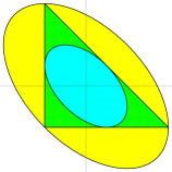
Figure 1. $\textup{Inn}_{P}(0)$ and $\textup{Out}_{P}(0)$ for a triangle centered at the origin.

For $n=2$, plugging into the formula for the inner approximation we get

$$\textup{Inn}_{Q}(0)=\{(x,y):(3(x+y)-2)^{2}+16(x-y)^{2}\leq 16\},$$

while doing it for the outer approximation yields

$$\textup{Out}_{Q}(0)=\{(x,y):3(x+y-1)^{2}+(x-y)^{2}\leq 12\}.$$

So we can see that while $\textup{Out}_{Q}(0)$ is simply a translation of the previous one, $\textup{Inn}_{Q}(0)$ has changed considerably as can be seen in Figure 2.

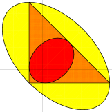
Figure 2. $\textup{Inn}_{Q}(0)$ and $\textup{Out}_{Q}(0)$ for a triangle not centered at the origin.

2.4. Closedness of $\textup{Inn}_{P}(A)$

It is easy to see that $\textup{Out}_{P}(B)$ is closed and bounded. Indeed, since ${\mathbbm{1}}$ lies in the interior of $\mathcal{O}_{in}^{v}$ which is the polar of $\mathcal{O}_{out}^{v}$, for every $z\in\mathcal{O}_{out}^{v}$, ${\mathbbm{1}}^{T}z>0$. Therefore, there is no $z\in\mathcal{O}_{out}^{v}$ such that ${\mathbbm{1}}^{T}(\lambda z)=\lambda({\mathbbm{1}}^{T}z)\leq 1$ for all $\lambda>0$ and so, $\{z\in\mathcal{O}_{out}^{v}\,:\,{\mathbbm{1}}^{T}z\leq 1\}$ is bounded. It is closed since $\mathcal{O}_{out}^{v}$ is closed. Further, $\{z\in\mathcal{O}_{out}^{v}\,:\,{\mathbbm{1}}^{T}z\leq 1,\,B(z)\in K\}$ is also compact since $B^{-1}(K)\subset\mathbb{R}^{v}$ is closed as $B$ is a linear map and $K$ is closed. Therefore, $\textup{Out}_{P}(B)$ is compact since it is the linear image of a compact set. The set $\textup{Inn}_{P}(A)$ is bounded since it is contained in the polytope $P$. We will also see in Proposition 2.20 that it has an interior. However, $\textup{Inn}_{P}(A)$ may not be closed.

Example 2.11.

Consider the three dimensional cone

$$K=\left\{(a,b,t)\in\mathbb{R}^{3}\ :\ \begin{pmatrix}a+b&0&2(a-b)\\ 0&t&2(a+b)-t\\ 2(a-b)&2(a+b)-t&t\end{pmatrix}\succeq 0\right\},$$

and take $A^{*}$ to be the map sending $(a,b,t)$ to $(a,b,0)$. Then,

$$A^{*}(K)=\{(x,y,0)\ :x>0,y>0\}\cup\{(0,0,0)\}.$$

For any triangle $P\subset\mathbb{R}^{2}$ given by ${1}-H^{*}(x)\geq 0$ we then have that

$$\textup{Inn}_{P}(A)=\left\{x\in\mathbb{R}^{2}\,:\,{1}-H^{*}(x)\in\mathcal{O}_{in}^{3}+A^{*}(K)\right\}.$$

Since $\mathcal{O}_{in}^{3}$ is a second order cone that is strictly contained in $\mathbb{R}^{3}_{+}$ and $A^{*}(K)$ has the description given above, the cone $\mathcal{O}_{in}^{3}+A^{*}(K)$ is not closed. The set $\textup{Inn}_{P}(A)$ is an affine slice of this non-closed cone and therefore, may not be closed. Taking, for example, the triangle

$$P=\left\{(x,y)\in\mathbb{R}^{2}\,:\,\begin{pmatrix}1-x\\ 1-y\\ 1+x+y\end{pmatrix}\geq 0\right\},$$

$$\textup{Inn}_{P}(A)=\left\{(x,y)\in\mathbb{R}^{2}\,:\,(1-x,1-y,1+x+y)\in\mathcal{O}_{in}^{3}+A^{*}(K)\right\},$$

which is not closed, as can be seen in Figure 3.

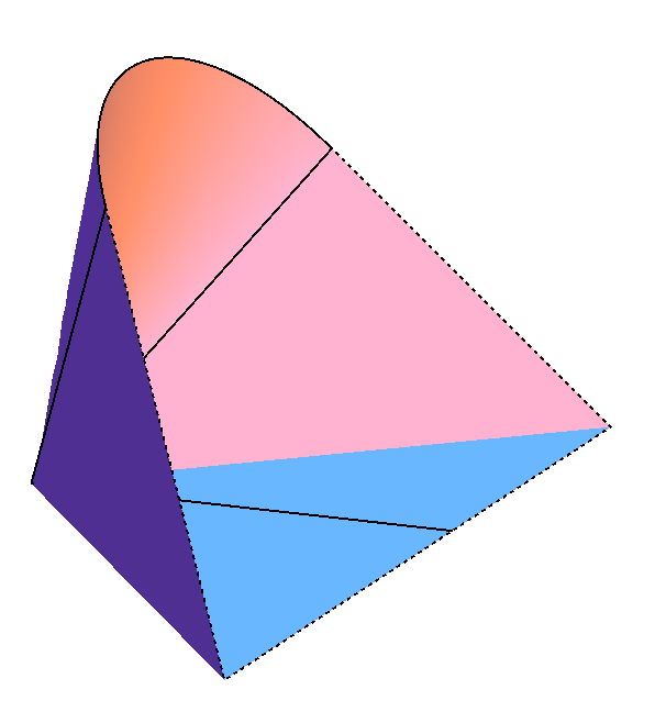
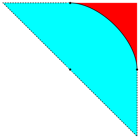
Figure 3. Affine slice of $\mathcal{O}_{in}^{3}+A^{*}(K)$, and the corresponding projection $\textup{Inn}_{P}(A)$.

Notice that in this example, $A$ is a nonnegative $K^{\ast}$-map, but $A^{\ast}(K)$ is not closed.

Remark 2.12.

If $A^{\ast}(K)$ is closed, then $\mathcal{O}_{in}^{f}+A^{\ast}(K)$ will be closed by [16, Corollary 9.12] since both cones are closed, and contained in $\mathbb{R}^{f}_{+}$, which means that there is no direction of recession of one cone whose opposite is a direction of recession of the other cone. If $\mathcal{O}_{in}^{f}+A^{\ast}(K)$ is closed then $\textup{Inn}_{P}(A)$ will be closed since it is an affine slice of $\mathcal{O}_{in}^{f}+A^{\ast}(K)$.

We now discuss results from [13] and [14] that give conditions under which $A^{\ast}(K)$ is closed.

Definition 2.13.

[13, Definition 1.1], [3] A closed convex cone $C$ is nice if $C^{\ast}+F^{\perp}$ is closed for all faces $F$ of $C$.

Nonnegative orthants, positive semidefinite cones, and second order cones are all nice. Given a convex set $C$, let $\textup{ri }C$ denote the relative interior of $C$. For $x\in C$, define

$$\textup{dir}(x,C)=\{y\,:\,x+\varepsilon y\in C\textup{ for some }\varepsilon>0\}$$

and $\textup{cl}(\textup{dir}(x,C))$ denote the closure of $\textup{dir}(x,C)$. For example, if $C\subset\mathbb{R}^{m}$ is a full-dimensional closed convex cone and $x$ is in the interior of $C$, then $\textup{dir}(x,C)=\mathbb{R}^{m}$. If $x\in\textup{ri }F$ for a face $F$ of $C$, then $\textup{dir}(x,C)$ contains the linear span of $F$ and hence, $\textup{cl}(\textup{dir}(x,C))\backslash\textup{dir}(x,C)$ does not contain the linear span of $F$.

Theorem 2.14.

[14, Theorem 1] Let $M$ be a linear map, $C$ a nice cone and $x\in\textup{ri }(C\cap\textup{range}(M))$. Then $M^{\ast}C^{\ast}$ is closed if and only if $\textup{range}(M)\cap(\textup{cl}(\textup{dir}(x,C))\backslash\textup{dir}(x,C))=\emptyset$.

Corollary 2.15.

If $K^{\ast}$ is a nice cone and $A$ is a nonnegative $K^{\ast}$-map, then both $A^{\ast}(K)$ and $\textup{Inn}_{P}(A)$ are closed.

Proof:   Since $A$ is a nonnegative $K^{\ast}$-map, $A$ sends $e_{i}^{\ast}\in(\mathbb{R}^{f})^{\ast}$ to $a_{i}\in K^{\ast}$. Therefore, $\textup{range}(A)$ is contained in the linear span of a face of $K^{\ast}$. Let $F$ be a minimal such face. If $x\in\textup{ri }(K^{\ast}\cap\textup{range}(A))$, then $x$ lies in $\textup{ri }F$ which means that $\textup{cl}(\textup{dir}(x,K^{\ast}))\backslash\textup{dir}(x,K^{\ast})$ does not contain the linear span of $F$ and hence does not contain $\textup{range}(A)$. This implies that $\textup{range}(A)\cap(\textup{cl}(\textup{dir}(x,K^{\ast}))\backslash\textup{dir}(x,K^{\ast}))=\emptyset$ and $A^{\ast}(K)$ is closed by Theorem 2.14. By Remark 2.12, it follows that $\textup{Inn}_{P}(A)$ is closed. $\square$

Remark 2.16.

By Corollary 2.15, $\textup{Inn}_{P}(A)$ is closed when $K$ is a nonnegative orthant, psd cone or a second order cone. Since these are precisely the cones that are of interest to us in this paper, we will assume that $\textup{Inn}_{P}(A)$ is closed in the rest of this paper. While this assumption will be convenient in the proofs of several forthcoming results, we note that the results would still be true if we were to replace $\textup{Inn}_{P}(A)$ by its closure everywhere.

2.5. Polarity

We now show that our approximations behave nicely under polarity. Recall that the polar of the polytope $P\subset\mathbb{R}^{n}$ is the polytope $P^{\circ}=\{y\in(\mathbb{R}^{n})^{\ast}\,:\,\langle y,x\rangle\leq 1,\,\,\forall\,\,x\in P\}$. The face lattices of $P$ and $P^{\circ}$ are anti-isomorphic. In particular, if $P=\{x\in\mathbb{R}^{n}\,:\,H^{T}x\leq{\mathbbm{1}}\}$ with vertices $p_{1},\ldots,p_{v}$ as before, then the facet inequalities of $P^{\circ}$ are $\langle y,p_{i}\rangle\leq 1$ for all $i=1,\ldots,v$ and the vertices are $h_{1},\ldots,h_{f}$. Therefore, given a nonnegative $K^{\ast}$-map $A:(\mathbb{R}^{f})^{\ast}\rightarrow(\mathbb{R}^{m})^{\ast}$ and a nonnegative $K$-map $B:\mathbb{R}^{v}\rightarrow\mathbb{R}^{m}$ we can use them, as above, to define approximations for $P^{\circ}$, $\textup{Inn}_{P^{\circ}}(B)$ and $\textup{Out}_{P^{\circ}}(A)$, since facets and vertices of $P$ and $P^{\circ}$ exchange roles. By applying polarity again, we potentially get new (different) outer and inner approximations of $P$ via Proposition 2.8. We now prove that in fact, we recover the same approximations, and so in a sense, the approximations are dual to each other.

As noted in Remark 2.16, we are assuming that $\textup{Inn}_{P}(A)$ is closed.

Theorem 2.17.

Let $P$ be a polytope, $A$ a nonnegative $K^{\ast}$-map and $B$ a nonnegative $K$-map as before. Then,

$$\textup{Out}_{P^{\circ}}(A)=(\textup{Inn}_{P}(A))^{\circ},$$

and equivalently,

$$\textup{Inn}_{P^{\circ}}(B)=(\textup{Out}_{P}(B))^{\circ}.$$

Proof:   Note that the two equalities are equivalent as one can be obtained from the other by polarity. Therefore, we will just prove the first statement. For notational convenience, we identify $\mathbb{R}^{n}$ and its dual. By definition,

$$(\textup{Inn}_{P}(A))^{\circ}=\{z\in\mathbb{R}^{n}\,:\,z^{T}x\leq 1\;\,\forall\,x\in\textup{Inn}_{P}(A)\}.$$

Consider then the problem

$$\textup{max }\{z^{T}x\,:\,x\in\textup{Inn}_{P}(A)\}=\textup{max }\{z^{T}x\,:\,{\mathbbm{1}}-H^{\ast}(x)-A^{\ast}(y)\in\mathcal{O}_{in}^{f},\,\,y\in K\}.$$

This equals the problem

$$\textup{max}_{x,y\in K}\,\textup{min}_{p\in(\mathcal{O}_{in}^{f})^{*}}\{z^{T}x+p^{T}({\mathbbm{1}}-H^{\ast}(x)-A^{\ast}(y))\}.$$

Strong duality [4] holds since the original problem $\textup{max }\{z^{T}x\,:\,x\in\textup{Inn}_{P}(A)\}$ is a convex optimization problem and $\textup{Inn}_{P}(A)$ has an interior as we will see in Proposition 2.20. This allows us to switch the order of min and max, to obtain

$$\textup{min}_{p\in(\mathcal{O}_{in}^{f})^{*}}\,\textup{max}_{x,y\in K}\{{\mathbbm{1}}^{T}p+x^{T}(z-H(p))-A(p)^{T}y\}.$$

For this max to be bounded above, we need $z=H(p)$ since $x$ is unrestricted, and $A(p)\in K^{\ast}$ since $y\in K$. Therefore, using $(\mathcal{O}_{in}^{f})^{*}=\mathcal{O}_{out}^{f}$, we are left with

$$\textup{min}_{p}\{{\mathbbm{1}}^{T}p\,:\,p\in\mathcal{O}_{out}^{f},\,\,z=H(p),\,\,A(p)\in K^{\ast}\}.$$

Looking back at the definition of $(\textup{Inn}_{P}(A))^{\circ}$, we get

$$(\textup{Inn}_{P}(A))^{\circ}=\{H(p)\,:\,p\in\mathcal{O}_{out}^{f},\,\,{\mathbbm{1}}^{T}p\leq 1,\,\,A(p)\in K^{\ast}\}$$

which is precisely $\textup{Out}_{P^{\circ}}(A)$. $\square$

2.6. Efficient representation

There would be no point in defining approximations of $P$ if they could not be described in a computationally efficient manner. Remarkably, the orthogonal invariance of the $2$-norm constraints in the definition of $\textup{Inn}_{P}(\cdot)$ and $\textup{Out}_{P}(\cdot)$ will allow us to compactly represent the approximations via second order cones (SOC), with a problem size that depends only on the conic rank $m$ (the affine dimension of $K$), and not on the number of vertices/facets of $P$. This feature is specific to our approximation and is of key importance, since the dimensions of the codomain of $A^{\ast}$ and the domain of $B$ can be exponentially large.

We refer to any set defined by a $k\times k$ positive semidefinite matrix $Q\succeq 0$ and a vector $a\in\mathbb{R}^{k}$ of the form

$$\{z\in\mathbb{R}^{k}\,:\,\|Q^{\frac{1}{2}}z\|\leq a^{T}z\}$$

as a $k$-second order cone or $\textup{SOC}_{k}$. Here $Q^{\frac{1}{2}}$ refers to a $k\times k$ matrix that is a square root of $Q\succeq 0$, i.e., $Q=(Q^{\frac{1}{2}})^{T}Q^{\frac{1}{2}}$. Suppose $M\in\mathbb{R}^{p\times k}$ is a matrix with $p\gg k$. Then $\|Mx\|^{2}=x^{T}M^{T}Mx=x^{T}Qx=\|Q^{\frac{1}{2}}x\|^{2}$ where $Q=M^{T}M$. Therefore, the expression $\|Mx\|$ (which corresponds to a 2-norm condition on $\mathbb{R}^{p}$) is equivalent to a 2-norm condition on $\mathbb{R}^{k}$ (and $k\ll p$). Notice that such a property is not true, for instance, for any $\ell_{q}$ norm for $q\not=2$.

We use this key orthogonal invariance property of $2$-norms to represent our approximations efficiently via second-order cones. Recall from the introduction that a convex set $C\subset\mathbb{R}^{n}$ has a $K$-lift, where $K\subset\mathbb{R}^{m}$ is a closed convex cone, if there is some affine subspace $L\subset\mathbb{R}^{m}$ and a linear map $\pi\,:\,\mathbb{R}^{m}\rightarrow\mathbb{R}^{n}$ such that $C=\pi(K\cap L)$. A set of the form $K^{\prime}=\{z\in\mathbb{R}^{k}\,:\,\|Q^{\frac{1}{2}}z\|_{2}\leq a_{0}+a^{T}z\}$ where the right-hand side is affine can be gotten by slicing its homogenized second order cone

$$\left\{(z_{0},z)\in\mathbb{R}^{k+1}\,:\,\left\|\left(\begin{array}[]{cc}0&0\\ 0&Q^{\frac{1}{2}}\end{array}\right)\left(\begin{array}[]{c}z_{0}\\ z\end{array}\right)\right\|\leq a_{0}z_{0}+a^{T}z\right\}$$

with the affine hyperplane $\{(z_{0},z)\in\mathbb{R}^{1+k}\,:\,z_{0}=1\}$ and projecting onto the $z$ variables. In other words, $K^{\prime}$ has a $\textup{SOC}_{k+1}$-lift.

Theorem 2.18.

Let $P\subseteq\mathbb{R}^{n}$ be a polytope, $K\subseteq\mathbb{R}^{m}$ a closed convex cone and $A$ and $B$ nonnegative $K^{\ast}$ and $K$-maps respectively. Then the convex sets $\textup{Inn}_{P}(A)$ and $\textup{Out}_{P}(B)$ have $K\times\textup{SOC}_{(n+m+2)}$-lifts.

Proof:   Set $M$ to be the $f\times(n+m+1)$ concatenated matrix $\left[H^{\ast}\,\,A^{\ast}\,\,\mathbbm{-1}\right]$. Then, using Definition 2.7, the characterization in Remark 2.6 and $Q:=M^{T}M$, we have

$$\begin{array}[]{lcl}\textup{Inn}_{P}(A)&=&\left\{x\in\mathbb{R}^{n}\,:\,\exists y\in K,\xi\in\mathbb{R}\textup{ s.t. }\left\|M\left(x^{T}\,\,y^{T}\,\,\xi\right)^{T}\right\|\leq 1-\xi\right\}\\ &=&\left\{x\in\mathbb{R}^{n}\,:\,\exists y\in K,\xi\in\mathbb{R}\textup{ s.t. }\|Q^{\frac{1}{2}}\left(x^{T}\,\,y^{T}\,\,\xi\right)^{T}\|\leq 1-\xi\right\}.\end{array}$$

From the discussion above, it follows that $\textup{Inn}_{P}(A)$ is the projection onto the $x$ variables of points $(z;x_{0},x,y,\xi)\in K\times\textup{SOC}_{n+m+2}$ such that $z=y$ and $x_{0}=1$ and so $\textup{Inn}_{P}(A)$ has a $K\times\textup{SOC}_{n+m+2}$-lift.

The statement for $\textup{Out}_{P}(B)$ follows from Theorem 2.17 and the fact that if a convex set $C\subset\mathbb{R}^{n}$ with the origin in its interior has a $K$-lift, then its polar has a $K^{\ast}$-lift [8]. We also use the fact that the dual of a $\textup{SOC}_{k}$ is another $\textup{SOC}_{k}$ cone. $\square$

Note that the lifting dimension is independent of $f$, the number of facets of $P$, which could be very large compared to $n$. A slightly modified argument can be used to improve this result by 1, and show that a $K\times\textup{SOC}_{(n+m+1)}$-lift always exists.

2.7. Approximation quality

The final question we will address in this section is how good an approximation $\textup{Inn}_{P}(A)$ and $\textup{Out}_{P}(B)$ are of the polytope $P$. We assume that $A^{\ast}(K)$ is closed which implies (by Remark 2.12) that both $\mathcal{O}_{in}^{f}+A^{\ast}(K)$ and $\textup{Inn}_{P}(A)$ are closed.

One would like to prove that if we start with a good approximate $K$-factorization of the slack matrix $S$ of $P$, we would get good approximate lifts of $P$ from our definitions. This is indeed the case as we will show. Recall that our approximations $\textup{Inn}_{P}(A)$ and $\textup{Out}_{P}(B)$ each depend on only one of the factors $A$ or $B$. For this reason, ideally, the goodness of these approximations should be quantified using only the relevant factor. Our next result presents a bound in this spirit.

Definition 2.19.

For $x\in\mathbb{R}^{f}$, let $\mu(x):=\textup{min}\{t\geq 0\,:\,x+t{\mathbbm{1}}\in\mathcal{O}_{in}^{f}+A^{\ast}(K)\}$.

Note that $\mu(x)$ is well defined since $\mathcal{O}_{in}^{f}+A^{\ast}(K)$ is closed and ${\mathbbm{1}}$ lies in the interior of $\mathcal{O}_{in}^{f}+A^{\ast}(K)$. Also, $\mu(x)=0$ for all $x\in\mathcal{O}_{in}^{f}+A^{\ast}(K)$.

Proposition 2.20.

For $\varepsilon=\textup{max}_{i}(\mu(S(e_{i}))$, $\frac{P}{1+\varepsilon}\subseteq\textup{Inn}_{P}(A)$.

Proof:   It suffices to show that $\frac{p}{1+\varepsilon}\in\textup{Inn}_{P}(A)$ where $p=V(e_{i})$ is a vertex of $P$. By the definition of $\varepsilon$, we have that $\varepsilon{\mathbbm{1}}+S(e_{i})\in\mathcal{O}_{in}^{f}+A^{\ast}(K)$ and hence, $\varepsilon{\mathbbm{1}}+{\mathbbm{1}}-H^{\ast}V(e_{i})\in\mathcal{O}_{in}^{f}+A^{\ast}(K)$. Therefore, ${\mathbbm{1}}-H^{\ast}(\frac{p}{1+\varepsilon})\in\mathcal{O}_{in}^{f}+A^{\ast}(K)$ and hence, $\frac{p}{1+\varepsilon}\in\textup{Inn}_{P}(A)$. $\square$

From this proposition one sees that the approximation factor improves as $A^{\ast}(K)$ gets bigger. While geometrically appealing, this bound is not very convenient from a computational viewpoint. Therefore, we now write down a simple, but potentially weaker, result based on an alternative error measure $\xi(\cdot)$ defined as follows.

Definition 2.21.

For $x\in\mathbb{R}^{f}$, define $\xi(x):=\textup{min}\,\{t\geq 0\,:\,x+t{\mathbbm{1}}\in\mathcal{O}_{in}^{f}\}$.

Again, $\xi(\cdot)$ is well-defined since $\mathcal{O}_{in}^{f}$ is closed and ${\mathbbm{1}}$ is in its interior. Also, $\mu(x)\leq\xi(x)$ for all $x\in\mathbb{R}^{f}$. Setting $t=\|x\|$ in Remark 2.6, we see that for any $x\in\mathbb{R}^{f}$, $x+\|x\|\cdot{\mathbbm{1}}\in\mathcal{O}_{in}^{f}$ which implies that $\xi(x)\leq\|x\|$. We also remark that $\xi(x)$ can be computed easily as follows.

Remark 2.22.

For $0\neq x\in\mathbb{R}^{f}$, $f\geq 2$,

$$\xi(x)=\textup{max}\left\{0,\,\,\|x\|\cdot\alpha\left(\frac{{\mathbbm{1}}^{T}x}{\sqrt{f}\|x\|}\right)\right\},$$

where $\alpha(s):=(\sqrt{(f-1)(1-s^{2})}-s)/\sqrt{f}$, and $\xi(0)=0$.

Using $\xi(\cdot)$ we will now provide a more convenient version of Proposition 2.20 based only on the factorization error.

Lemma 2.23.

Let $A:(\mathbb{R}^{f})^{\ast}\rightarrow(\mathbb{R}^{m})^{\ast}$ be a nonnegative $K^{\ast}$-map and $B:\mathbb{R}^{v}\rightarrow\mathbb{R}^{m}$ be a nonnegative $K$-map. Let $\Delta=S-A^{\ast}\circ B$. Then, $\frac{1}{1+\varepsilon}P\subseteq\textup{Inn}_{P}(A)$, for $\varepsilon=\textup{max}_{i}\,\xi(\Delta(e_{i}))$.

Proof:   Note that $\mu(S(e_{i}))=\textup{min}\{t\geq 0\,:\,\exists\,\,u\in A^{\ast}(K)\textup{ s.t. }S(e_{i})-u+t{\mathbbm{1}}\in\mathcal{O}_{in}^{f}\}$. Since $B(e_{i})\in K$, we have that $A^{\ast}(B(e_{i}))\in A^{\ast}(K)$. Therefore,

$$\mu(S(e_{i}))\leq\textup{min}\{t\geq 0\,:\,\underbrace{S(e_{i})-A^{\ast}(B(e_{i}))}_{\Delta(e_{i})}+t{\mathbbm{1}}\in\mathcal{O}_{in}\}=\xi(\Delta(e_{i})).$$

$\square$

We immediately get our main result establishing the connection between the quality of the factorization and the quality of the approximations. For simplicity, we state it using the simplified upper bound $\xi(x)\leq\|x\|$.

Proposition 2.24.

Let $A:(\mathbb{R}^{f})^{\ast}\rightarrow(\mathbb{R}^{m})^{\ast}$ be a nonnegative $K^{\ast}$-map and $B:\mathbb{R}^{v}\rightarrow\mathbb{R}^{m}$ be a nonnegative $K$-map. Let $\Delta:=S-A^{\ast}\circ B$ be the factorization error. Then,

1. $\frac{1}{1+\varepsilon}P\subseteq\textup{Inn}_{P}(A)$, for $\varepsilon=\|\Delta\|_{1,2}$;

2. $\textup{Out}_{P}(B)\subseteq(1+\varepsilon)P$, for $\varepsilon=\|\Delta\|_{2,\infty}$,

where $\|\Delta\|_{1,2}=\textup{max}_{i}\|\Delta(e_{i})\|$ is the induced $\ell_{1},\ell_{2}$ norm and $\|\Delta\|_{2,\infty}=\textup{max}_{i}\|\Delta^{\ast}(e_{i}^{\ast})\|$ is the induced $\ell_{2},\ell_{\infty}$ norm of the factorization error.

Proof:   By Theorem 2.17, the two statements are equivalent. The proof now follows from Lemma 2.23. $\square$

This means that if we start with $A$ and $B$ forming a $K$-factorization of a nonnegative $S^{\prime}$ which is close to the true slack matrix $S$, we get a $(1+\|S-S^{\prime}\|_{1,2})$-approximate inner approximation of $P$, as well as a $(1+\|S-S^{\prime}\|_{2,\infty})$-approximate outer approximation of $P$. Thus, good approximate factorizations of $S$ do indeed lead to good approximate lifts of $P$.

Example 2.25.

Consider the square given by the inequalities $1\pm x\geq 0$ and $1\pm y\geq 0$ with vertices $(\pm 1,\pm 1)$. By suitably ordering facets and vertices, this square has slack matrix

$$S=\left(\begin{array}[]{cccc}2&2&0&0\\ 0&2&2&0\\ 0&0&2&2\\ 2&0&0&2\end{array}\right).$$

Let $A:(\mathbb{R}^{4})^{\ast}\rightarrow(\mathbb{R}^{2})^{\ast}$ and $B\,:\,\mathbb{R}^{4}\rightarrow\mathbb{R}^{2}$ be the nonnegative maps given by the matrices

$$A=\left(\begin{array}[]{cccc}4/3&4/3&0&0\\ 0&0&4/3&4/3\end{array}\right)\,\,\textup{ and }\,\,B=\left(\begin{array}[]{cccc}1&1&1&0\\ 1&0&1&1\end{array}\right).$$

Then $A$ and $B$ are nonnegative $\mathbb{R}^{2}_{+}=(\mathbb{R}^{2}_{+})^{\ast}$ maps and

$$A^{T}B=\left(\begin{array}[]{cccc}4/3&4/3&4/3&0\\ 4/3&4/3&4/3&0\\ 4/3&0&4/3&4/3\\ 4/3&0&4/3&4/3\end{array}\right).$$

It is easy to check that $\|S-A^{T}B\|_{1,2}=\frac{2}{3}\sqrt{10}$ while $\|S-A^{T}B\|_{2,\infty}=2\sqrt{\frac{2}{3}}$. So by Proposition 2.24 this implies that

$$\frac{1}{1+\frac{2}{3}\sqrt{10}}P\subseteq\textup{Inn}_{P}(A)\subseteq P\subseteq\textup{Out}_{P}(B)\subseteq(1+2\sqrt{\textstyle\frac{2}{3}})P.$$

If we use instead Lemma 2.23, we can get the slightly better quality bounds

$$\frac{1}{\frac{4}{3}+\sqrt{3}}P\subseteq\textup{Inn}_{P}(A)\subseteq P\subseteq\textup{Out}_{P}(B)\subseteq(1+\sqrt{2})P.$$

Finally, if we use directly Proposition 2.20, it is possible in this case to compute explicitly the true bounds

$$\frac{1}{\sqrt{3}}P\subseteq\textup{Inn}_{P}(A)\subseteq P\subseteq\textup{Out}_{P}(B)\subseteq\sqrt{3}P.$$

In Figure 4 we can see the relative quality of all these bounds.

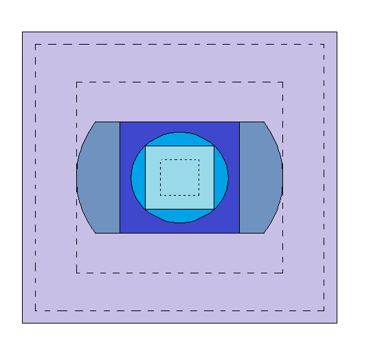
Figure 4. $\textup{Inn}_{P}(A)$, $P$ and $\textup{Out}_{P}(B)$, as well as all the guaranteed approximations.

3. Special Cases

In this section we relate our inner approximation to Dikin’s ellipsoid, a well known inner approximation to a polytope that arises in the context of interior point methods. We also compute $\textup{Inn}_{P}(A)$ and $\textup{Out}_{P}(B)$ from a nonnegative factorization of the closest rank one approximation of the slack matrix of $P$. As we will see, these are the two simplest possible approximations of a polytope, and correspond to specific choices for the factors $A$ and $B$.

3.1. Dikin’s ellipsoid

Recall that $\textup{Inn}_{P}(0)$ is an ellipsoidal inner approximation of $P$ that is intrinsic to $P$ and does not depend on any approximate factorization of the slack matrix of $P$ through any cone. A commonly used inner approximation of a polytope is Dikin’s ellipsoid defined as follows. Let $P=\{x\in\mathbb{R}^{n}\,:\,H^{T}x\leq{\mathbbm{1}}\}$ be a polytope as before and let $h_{1},\ldots,h_{f}$ be the columns of $H$. Define

$$\Gamma_{P}(x):=\sum_{i=1}^{f}\frac{h_{i}h_{i}^{T}}{(1-\langle h_{i},x\rangle)^{2}},$$

which is the Hessian of the standard logarithmic barrier function $\psi(x):=-\sum_{i=1}^{f}\log(1-\langle h_{i},x\rangle)$ associated to $P$. If $x_{0}$ is in the interior of $P$, then the Dikin ellipsoid centered at $x_{0}$ and of radius $r$, is the set

$$D_{x_{0}}^{r}:=\{x\in\mathbb{R}^{n}\,:\,(x-x_{0})^{T}\Gamma_{P}(x_{0})(x-x_{0})\leq r^{2}\}.$$

It can be checked that $D_{x_{0}}^{1}\subseteq P$ (see Theorem 2.1.1 in [11]). Further, since Dikin’s ellipsoid is invariant under translations, we may assume that $x_{0}=0$, and then

$$D_{0}^{1}=\left\{x\in\mathbb{R}^{n}\,:\,x^{T}\left(\sum_{i=1}^{f}{h_{i}h_{i}^{T}}\right)x\leq 1\right\}=\left\{x\in\mathbb{R}^{n}\,:\,\ \|H^{T}x\|\leq 1\right\}.$$

Recall that

$$\textup{Inn}_{P}(0) =\left\{x\in\mathbb{R}^{n}\,:\,{\mathbbm{1}}-H^{T}x\in\mathcal{O}_{in}^{f}\right\}=\left\{x\in\mathbb{R}^{n}\,:\,\exists t\in\mathbb{R}\mbox{ s.t. }\|(t-1){\mathbbm{1}}+H^{T}x\|\leq t\right\},$$

where we used the characterization of $\mathcal{O}_{in}^{f}$ given in Remark 2.6. Choosing $t=1$, we see that $D_{0}^{1}\subseteq\textup{Inn}_{P}(0)\subseteq P$. This inclusion is implicit in the work of Sturm and Zhang [19].

If the origin is also the analytic center of $P$ (i.e., the minimizer of $\psi(x)$), then we have that $P\subseteq\sqrt{f(f-1)}D_{0}^{1}$ where $f$ is the number of inequalities in the description of $P$; see [18] and [4, Section 8.5.3]. Also, in this situation, the first order optimality condition on $\psi(x)$ gives that $\sum_{i=1}^{f}h_{i}=0$, and as a consequence, $f=\sum_{i=1}^{f}(1-\langle h_{i},p\rangle)$ for all vertices $p$ of $P$. In other words, every column of the slack matrix sums to $f$. This implies an analogous (slightly stronger) containment result for $\textup{Inn}_{P}(0)$.

Corollary 3.1.

If the origin is the analytic center of the polytope $P$, then

$$\textup{Inn}_{P}(0)\subseteq P\subseteq(f-1)\,\textup{Inn}_{P}(0),$$

furthermore, if $P$ is centrally symmetric

$$\textup{Inn}_{P}(0)\subseteq P\subseteq\sqrt{f-1}\,\textup{Inn}_{P}(0).$$

Proof:   This follows from Lemma 2.23 and Remark 2.22, by using the fact that if $S$ is the slack matrix of $P$ then $\|S(e_{i})\|\leq{\mathbbm{1}}^{T}S(e_{i})=f$. In this case, for $w=S(e_{i})$, we have $\frac{\mathbbm{1}^{T}w}{\sqrt{f}\|w\|}\geq\frac{1}{\sqrt{f}}$ and thus, since $\alpha(s)$ is decreasing for $s\geq-\frac{1}{\sqrt{f}}$, we get $\xi(w)=\|w\|\alpha(\frac{\mathbbm{1}^{T}w}{\sqrt{f}\|w\|})\leq\|w\|\alpha(\frac{1}{\sqrt{f}})\leq f\cdot\frac{f-2}{f}=f-2$, from where the first result follows.

For the second result, note that if $P$ is centrally symmetric, for every facet inequality $1-\langle h_{j},x\rangle\geq 0$ we have also the facet inequality $1+\langle h_{j},x\rangle\geq 0$, which implies

$$\|S(e_{i})\|=\sqrt{\frac{1}{2}\sum_{j=1}^{f}\left[(1-\langle h_{j},p_{i}\rangle)^{2}+(1+\langle h_{j},p_{i}\rangle)^{2}\right]}=\sqrt{f+\|H^{T}p_{i}\|^{2}}.$$

Using this fact together with ${\mathbbm{1}}^{T}S(e_{i})=f$, we get that $\xi(S(e_{i}))=\sqrt{\frac{f-1}{f}}\|H^{T}p_{i}\|-1$. Since $\mathbbm{1}-H^{T}p_{i}$ and $\mathbbm{1}+H^{T}p_{i}$ are both nonnegative, all entries in $H^{T}p_{i}$ are smaller than one in absolute value. Hence, $\|H^{T}p_{i}\|\leq\sqrt{f}$, concluding the proof. $\square$

Remark 3.2.

It was shown by Sonnevend [18] that when $x_{0}$ is the analytic center of $P$, $\sqrt{{f}/(f-1)}D_{x_{0}}^{1}\subseteq P$. By affine invariance of the result, we may assume that $x_{0}=0$, and in combination with the previously mentioned result from [18], we get

$$\sqrt{{f}/(f-1)}D_{0}^{1}\subseteq P\subseteq\sqrt{f(f-1)}D_{0}^{1}.$$

This implies that the Sonnevend ellipsoid, $\sqrt{{f}/(f-1)}D_{0}^{1}$, a slightly dialated version of the Dikin ellipsoid $D_{0}^{1}$, is also contained in $P$. Since $D_{0}^{1}=\{x\in\mathbb{R}^{n}\,:\,\|H^{T}x\|\leq{\mathbbm{1}}\}$, we get that $\sqrt{{f}/(f-1)}D_{0}^{1}=\{x\in\mathbb{R}^{n}\,:\,\|H^{T}x\|\leq\sqrt{{f}/(f-1)}\}$. On the other hand,

$$\begin{array}[]{lcl}\textup{Inn}_{P}(0)&=&\{x\in\mathbb{R}^{n}\,:\,{\mathbbm{1}}-H^{T}x\in\mathcal{O}_{in}^{f}\}\\ &=&\{x\in\mathbb{R}^{n}\,:\,\sqrt{f-1}\|{\mathbbm{1}}-H^{T}x\|\leq{\mathbbm{1}}^{T}({\mathbbm{1}}-H^{T}x)\}\\ &=&\{x\in\mathbb{R}^{n}\,:\,(f-1)\|H^{T}x\|^{2}\leq f-2(\sum h_{i})^{T}x+((\sum h_{i})^{T}x)^{2}\}.\end{array}.$$

When the origin is the analytic center of $P$, $\sum h_{i}=0$, and $\textup{Inn}_{P}(0)=\sqrt{{f}/(f-1)}D_{0}^{1}$, which makes the containment $\sqrt{{f}/{f-1}}D_{0}^{1}\subseteq P$ at most as strong as $\textup{Inn}_{P}(0)\subseteq P$. The containment $\textup{Inn}_{P}(0)\subseteq P$ holds whenever the origin is in $P$ while the Sonnevend containments require the origin to be the analytic center of $P$.

3.2. Singular value decomposition

Let $P$ be a polytope as before and suppose $S=U\Sigma V^{T}$ is a singular value decomposition of the slack matrix $S$ of $P$ with $U$ and $V$ orthogonal matrices and $\Sigma$ a diagonal matrix with the singular values of $S$ on the diagonal. By the Perron-Frobenius theorem, the leading singular vectors of a nonnegative matrix can be chosen to be nonnegative. Therefore, if $\sigma$ is the largest singular value of $S$, and $u$ is the first column of $U$ and $v$ is the first column of $V$ then $A=\sqrt{\sigma}u^{T}$ and $B=\sqrt{\sigma}v^{T}$ are two nonnegative matrices. By the Eckart-Young theorem, the matrix $A^{T}B=\sigma uv^{T}$ is the closest rank one matrix (in Frobenius norm) to $S$. We can also view $A^{T}B$ as an approximate $\mathbb{R}_{+}$-factorization of $S$ and thus look at the approximations $\textup{Inn}_{P}(A)=:\textup{Inn}_{P}^{\textrm{sing}}$ and $\textup{Out}_{P}(B)=:\textup{Out}_{P}^{\textrm{sing}}$ and hope that in some cases they may offer good compact approximations to $P$. Naturally, these are not as practical as $\textup{Inn}_{P}(0)$ and $\textup{Out}_{P}(0)$ since to compute them we need to have access to a complete slack matrix of $P$ and its leading singular vectors. We illustrate these approximations on an example.

Example 3.3.

Consider the quadrilateral with vertices $(1,0),(0,2),(-1,0)$ and $(0,-1/2)$. This polygon has slack matrix

$$S=\left[\begin{array}[]{cccc}0&5&2&0\\ 0&0&2&5/4\\ 2&0&0&5/4\\ 2&5&0&0\end{array}\right],$$

and by computing a singular value decomposition and proceeding as outlined above, we obtain the $1\times 4$ matrices

$$A=[1.9130,0.1621,0.1621,1.9130]\textup{ and }B=[0.5630,2.5951,0.5630,0.0550],$$

verifying

$$S^{\prime}=A^{T}B=\left[\begin{array}[]{cccc}1.0770&4.9644&1.0770&0.1051\\ 0.0912&0.4206&0.0912&0.0089\\ 0.0912&0.4206&0.0912&0.0089\\ 1.0770&4.9644&1.0770&0.1051\end{array}\right].$$

Computing $\textup{Inn}_{P}^{\textrm{sing}}$ and $\textup{Out}_{P}^{\textrm{sing}}$ we get the inclusions illustrated in Figure 5. Notice how these rank one approximations from leading singular vectors use the extra information to improve on the trivial approximations $\textup{Inn}_{P}(0)$ and $\textup{Out}_{P}(0)$. Notice also that since

$$\textup{Out}_{P}^{\textrm{sing}}=\textup{Out}_{P}(B)=\{V(z)\,:\,z\in\mathbb{R}^{4},\,\|z\|\leq{\mathbbm{1}}^{T}z\leq 1,\,Bz\geq 0\},$$

and $Bz\geq 0$ is a single linear inequality, $\textup{Out}_{P}^{\textrm{sing}}$ is obtained from $\textup{Out}_{P}(0)$ by imposing a new linear inequality. By polarity, $\textup{Inn}_{P}^{\textrm{sing}}$ is the convex hull of $\textup{Inn}_{P}(0)$ with a new point.

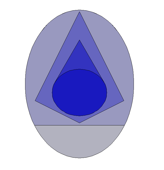
Figure 5. $\textup{Inn}_{P}(0)\subseteq\textup{Inn}_{P}^{\textrm{sing}}\subseteq P\subseteq\textup{Out}_{P}^{\textrm{sing}}\subseteq\textup{Out}_{P}(0)$.

4. Nested polyhedra and Generalized Slack Matrices

In this section, we consider approximate factorizations of generalized slack matrices and what they imply in terms of approximations to a pair of nested polyhedra. The results here can be seen as generalizations of results in Section 2.

Let $P\subset\mathbb{R}^{n}$ be a polytope with vertices $p_{1},\ldots,p_{v}$ and the origin in its interior, and $Q\subset\mathbb{R}^{n}$ be a polyhedron with facet inequalities $\langle h_{j},x\rangle\leq 1$, for $j=1,\ldots,f$, such that $P\subseteq Q$. The slack matrix of the pair $P,Q$ is the $f\times v$ matrix $S_{P,Q}$ whose $(i,j)$-entry is $1-\langle h_{i},p_{j}\rangle$. In the language of operators from Section 2, $S_{P,Q}$ can be thought of as an operator from $\mathbb{R}^{v}\rightarrow\mathbb{R}^{f}$ defined as $S_{P,Q}(x)=(\mathbbm{1}_{f\times v}-H_{Q}^{\ast}\circ V_{P})(x)$ where $V_{P}$ is the vertex operator of $P$ and $H_{Q}$ is the facet operator of $Q$. Every nonnegative matrix can be interpreted as such a generalized slack matrix after a suitable rescaling of its rows and columns, possibly with some extra rows and columns representing redundant points in $P$ and redundant inequalities for $Q$.

4.1. Generalized slack matrices and lifts

Yannakakis’ theorem about $\mathbb{R}^{m}_{+}$-lifts of polytopes can be extended to show that $S_{P,Q}$ has a $K$-factorization (where $K\subset\mathbb{R}^{m}$ is a closed convex cone), if and only if there exists a convex set $C$ with a $K$-lift such that $P\subseteq C\subseteq Q$. (For a proof in the case of $K=\mathbb{R}^{m}_{+}$, see [5, Theorem 1], and for $K=\mathcal{S}_{+}^{m}$ see [9]. Related formulations in the polyhedral situation also appear in [7, 12].) For an arbitrary cone $K$, there is a requirement that the $K$-lift of $C$ contains an interior point of $K$ [8, Theorem 1], but this is not needed for nonnegative orthants or psd cones, and we ignore this subtlety here.

Two natural convex sets with $K$-lifts that are nested between $P$ and $Q$ can be obtained as follows. For a nonnegative $K^{\ast}$-map $A\,:\,(\mathbb{R}^{f})^{\ast}\rightarrow(\mathbb{R}^{m})^{\ast}$ and a nonnegative $K$-map $B:\mathbb{R}^{v}\rightarrow\mathbb{R}^{m}$, define the sets:

$$C_{A} :=\left\{x\in\mathbb{R}^{n}\,:\,\exists\,y\in K\textup{ s.t. }{\mathbbm{1}}-H_{Q}^{\ast}(x)-A^{\ast}(y)=0\right\},$$

$$C_{B} :=\{V_{P}(z)\,:\,{\mathbbm{1}}^{T}z=1,\,\,B(z)\in K\}.$$

The sets $C_{A}$ and $C_{B}$ have $K$-lifts since they are obtained by imposing affine conditions on the cone $K$. From the definitions and Remark 2.9, it immediately follows that these containments hold:

$$P\subseteq\textup{Out}_{P}(B)\subseteq C_{B}\quad\textup{ and }\quad C_{A}\subseteq\textup{Inn}_{Q}(A)\subseteq Q.$$

As discussed in the introduction, the set $C_{A}$ could potentially be empty for an arbitrary choice of $A$. On the other hand, since $P\subseteq C_{B}$, $C_{B}$ is never empty. Thus in general, it is not true that $C_{B}$ is contained in $C_{A}$. However, in the presence of an exact factorization we get the following chain of containments.

Proposition 4.1.

When $S_{P,Q}=A^{\ast}\circ B$, we get $P\subseteq\textup{Out}_{P}(B)\subseteq C_{B}\subseteq C_{A}\subseteq\textup{Inn}_{Q}(A)\subseteq Q$.

Proof:   We only need to show that $C_{B}\subseteq C_{A}$. Let $V_{P}(z)\in C_{B}$, with ${\mathbbm{1}}_{v}^{T}z=1$ and $B(z)\in K$. Then choosing $y=B(z)$, we have that ${\mathbbm{1}}_{f}-H_{Q}^{\ast}(V_{P}(z))-A^{\ast}(B(z))={\mathbbm{1}}_{f}{\mathbbm{1}_{v}}^{T}z-H_{Q}^{\ast}(V_{P}(z))-A^{\ast}(B(z))=S_{P,Q}(z)-A^{\ast}(B(z))=0$ since $S_{P,Q}=A^{\ast}\circ B$. Therefore, $C_{B}\subseteq C_{A}$ proving the result. $\square$

Example 4.2.

To illustrate these inclusions, consider the quadrilateral $P$ with vertices $(1/2,0),(0,1),(-1/2,0),(0,-1)$, and the quadrilateral $Q$ defined by the inequalities $1-x\geq 0$, $1-x/2-y/2\geq 0$, $1+x\geq 0$ and $1+x/2+y/2\geq 0$. We have $P\subseteq Q$, and

$$S_{P,Q}=\frac{1}{4}\left(\begin{array}[]{cccc}2&4&6&4\\ 3&2&5&6\\ 6&4&2&4\\ 5&6&3&2\end{array}\right).$$

For $K=\mathbb{R}^{3}_{+}$ we can find an exact factorization for this matrix, such as the one given by

$$S_{P,Q}=A^{T}B=\left(\begin{array}[]{ccc}0&2&1\\ 0&1&\frac{3}{2}\\ 2&0&1\\ 2&1&\frac{1}{2}\end{array}\right)\left(\begin{array}[]{cccc}\frac{1}{2}&\frac{1}{2}&0&0\\ 0&\frac{1}{2}&\frac{1}{2}&0\\ \frac{1}{2}&0&\frac{1}{2}&1\end{array}\right).$$

In this example,

$$C_{A}=C_{B}=\left\{(x_{1},x_{2})\,:\,1-x_{2}\geq 0,1+2x_{1}+x_{2}\geq 0,1-2x_{1}+x_{2}\geq 0\right\}.$$

By computing $\textup{Inn}_{Q}(A)$ and $\textup{Out}_{P}(B)$ we can see as in Figure 6 that

$$P\subsetneq\textup{Out}_{P}(B)\subsetneq C_{B}=C_{A}\subsetneq\textup{Inn}_{Q}(A)\subsetneq Q.$$

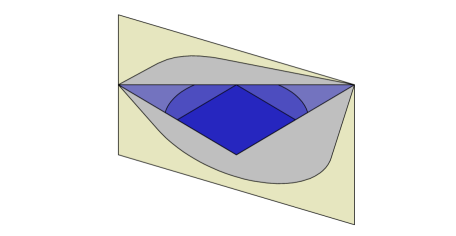
Figure 6. $P\subsetneq\textup{Out}_{P}(B)\subsetneq C_{B}=C_{A}\subsetneq\textup{Inn}_{Q}(A)\subsetneq Q$.

Note that if instead we pick the factorization

$$S_{P,Q}=A^{T}B=\left(\begin{array}[]{cccc}0&2&1&1\\ 0&1&\frac{3}{2}&0\\ 2&0&1&1\\ 2&1&\frac{1}{2}&2\end{array}\right)\left(\begin{array}[]{cccc}\frac{1}{2}&\frac{1}{2}&0&0\\ 0&\frac{1}{2}&\frac{1}{2}&0\\ \frac{1}{2}&0&\frac{1}{2}&1\\ 0&0&0&0\end{array}\right),$$

then $C_{A}\subsetneq C_{B}$ and we get the inclusions in Figure 7.

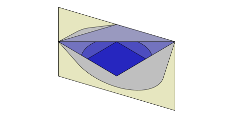
Figure 7. $P\subsetneq\textup{Out}_{P}(B)\subsetneq C_{B}\subsetneq C_{A}\subsetneq\textup{Inn}_{Q}(A)\subsetneq Q$.

4.2. Approximate Factorizations of $S_{P,Q}$

We now consider approximate factorizations of the generalized slack matrix $S_{P,Q}$ and provide three results about this situation. First, we generalize Proposition 2.24 to show that the quality of the approximations to $P$ and $Q$ is directly linked to the factorization error. Next we show how approximations to a pair of nested polytopes yield approximate $K$-factorizations of $S_{P,Q}$. We close with an observation on the recent inapproximability results in [5] in the context of this paper.

When we only have an approximate factorization of $S_{P,Q}$, we obtain a strict generalization of Proposition 2.24, via the same proof.

Proposition 4.3.

Let $A:(\mathbb{R}^{f})^{\ast}\rightarrow(\mathbb{R}^{m})^{\ast}$ a nonnegative $K^{\ast}$-map and $B:\mathbb{R}^{v}\rightarrow\mathbb{R}^{m}$ be a nonnegative $K$-map. Let $\Delta:=S_{P,Q}-A^{\ast}\circ B$ be the factorization error. Then,

1. $\frac{1}{1+\varepsilon}P\subseteq\textup{Inn}_{Q}(A)\subseteq Q$, for $\varepsilon=\|\Delta\|_{1,2}$.

2. $P\subseteq\textup{Out}_{P}(B)\subseteq(1+\varepsilon)Q$, for $\varepsilon=\|\Delta\|_{2,\infty}$.

So far we discussed how an approximate factorization of the slack matrix can be used to yield approximations of a polytope or a pair of nested polyhedra. It is also possible to go in the opposite direction in the sense that approximations to a pair of nested polyhedra $P\subseteq Q$ yield approximate factorizations of the slack matrix $S_{P,Q}$ as we now show.

Proposition 4.4.

Let $P\subseteq Q$ be a pair of polyhedra as before and $S_{P,Q}$ be its slack matrix. Suppose there exists a convex set $C$ with a $K$-lift such that $\alpha P\subseteq C\subseteq\beta Q$ for some $0<\alpha\leq 1$ and $\beta\geq 1$. Then there exists a $K$-factorizable nonnegative matrix $S^{\prime}$ such that $|(S^{\prime}-S_{P,Q})_{ij}|\leq\frac{\beta}{\alpha}-1$.

Proof:   Assume that the facet inequalities of $Q$ are of the form $\langle h_{j},x\rangle\leq 1$. Since $C$ has a $K$-lift, it follows from [8] that we can assign an element $b_{x}\in K$ to each point $x$ in $C$, and an element $a_{y}\in K^{\ast}$ to every valid inequality $y_{0}-\left<y,x\right>\geq 0$ for $C$, such that $\left<a_{y},b_{x}\right>=y_{0}-\left<y,x\right>$.

If $\alpha=\beta=1$, then $P\subseteq C\subseteq Q$, and since $C$ has a $K$-lift, $S_{P,Q}$ has a $K$-factorization and $S^{\prime}=S_{P,Q}$ gives the result. So we may assume that $\frac{\beta}{\alpha}>1$ and define $\eta>0$ such that $(1+\eta)\alpha=\beta$. If $1-\left<h,x\right>\geq 0$ defines a facet of $Q$, then $1+\eta-\frac{1}{\alpha}\left<h,x\right>\geq 0$ is a valid inequality for $(1+\eta)\alpha Q=\beta Q$, and is therefore a valid inequality for $C$. Hence, we can pick $a_{1},\ldots,a_{f}$ in $K^{*}$, one for each such inequality as mentioned above. Similarly, if $v$ is a vertex of $P$, then $\alpha v$ belongs to $C$ and we can pick $b_{1},\ldots,b_{v}$ in $K$, one for each $\alpha v$. Then,

$$\left<a_{i},b_{j}\right>=1+\eta-\frac{1}{\alpha}\left<h_{i},\alpha v_{j}\right>=\eta+(S_{P,Q})_{ij}.$$

The matrix $S^{\prime}$ defined by $S^{\prime}_{ij}:=\left<a_{i},b_{j}\right>$ yields the result. $\square$

Note that Proposition 4.4 is not a true converse of Proposition 4.3. Proposition 4.3 says that approximate $K$-factorizations of the slack matrix give approximate $K\times\textup{SOC}$-lifts of the polytope or pair of polytopes, while Proposition 4.4 says that an approximation of a polytope with a $K$-lift gives an approximate $K$-factorization of its slack matrix. We have not ruled out the existence of a polytope with no good $K$-liftable approximations but whose slack matrix has a good approximate $K$-factorization.

A recent result on the inapproximability of a polytope by polytopes with small lifts, come from the max clique problem, as seen in [5] (and strengthened in [6]). In [5], the authors prove that for $P(n)=\textup{COR}(n)=\textup{conv}\{bb^{T}\ |\ b\in\{0,1\}^{n}\}$ and

$$Q(n)=\{x\in\mathbb{R}^{n\times n}\ |\ \left<2\textup{diag}(a)-aa^{T},x\right>\leq 1,a\in\{0,1\}^{n}\},$$

and for any $\rho>1$, if $P(n)\subseteq C(n)\subseteq\rho Q(n)$ then any $\mathbb{R}^{m}_{+}$-lift of $C(n)$ has $m=2^{\Omega(n)}$. Therefore, one cannot approximate $P(n)$ within a factor of $\rho$ by any polytope with a small linear lift. This in turn says that the max clique problem on a graph with $n$ vertices cannot be approximated well by polytopes with small polyhedral lifts. In fact they also prove that even if $\rho=O(n^{\beta})$, for some $\beta\leq 1/2$, the size of $m$ grows exponentially.

The above result was proven in [5] by showing that the nonnegative rank of the slack matrix $S_{P(n),\rho Q(n)}$, denoted as $\textup{rank}_{+}(S_{P(n),\rho Q(n)})$, has order $2^{\Omega(n)}$. The matrix $S_{P(n),\rho Q(n)}$ is a very particular perturbation of $S_{P(n),Q(n)}$. It is not hard to see that the proof of Theorem 5 in [5] in fact shows that all nonnegative matrices in a small neighborhood of $S_{P(n),Q(n)}$ have high nonnegative rank.

Proposition 4.5.

Let $P(n)$ and $Q(n)$ be as above, and $0<\eta<1/2$. For any nonnegative matrix $S^{\prime}(n)$ such that $\|S_{P(n),Q(n)}-S^{\prime}(n)\|_{\infty}\leq\eta$, $\textup{rank}_{+}(S^{\prime}(n))=2^{\Omega(n)}$.

Since $\|S_{P(n),Q(n)}-S_{P(n),\rho Q(n)}\|_{\infty}=\rho-1$, Proposition 4.5 implies a version of the first part of the result in [5], i.e., that the nonnegative rank of $S_{P(n),\rho Q(n)}$ is exponential in $n$ (if only for $1<\rho<3/2$). Further, Proposition 4.5 also says that even if we allowed approximations of $P(n)$ in the sense of Proposition 4.3 (i,e., approximations with a $\mathbb{R}^{m}_{+}\times\textup{SOC}$-lift that do not truly nest between $P(n)$ and $Q(n)$), $m$ would not be small. Therefore, the result in [5] on the outer inapproximability of $P(n)$ by small polyhedra is robust in a very strong sense.

Acknowledgements: We thank Anirudha Majumdar for the reference to [19], and Cynthia Vinzant for helpful discussions about cone closures.

References

- [1] F. Alizadeh and D. Goldfarb. Second-order cone programming. Mathematical programming, 95(1):3–51, 2003.
- [2] G. Blekherman, P. A. Parrilo, and R. R. Thomas, editors. Semidefinite optimization and convex algebraic geometry, volume 13 of MOS-SIAM Series on Optimization. SIAM, 2012.
- [3] J. Borwein and H. Wolkowicz. Regularizing the abstract convex program. J. Math. Anal. Appl., 83(2):495–530, 1981.
- [4] S. Boyd and L. Vandenberghe. Convex Optimization. Cambridge University Press, 2004.
- [5] G. Braun, S. Fiorini, S. Pokutta, and D. Steurer. Approximation limits of linear programs (beyond hierarchies). In Foundations of Computer Science (FOCS), 2012 IEEE 53rd Annual Symposium on, pages 480–489. IEEE, 2012.
- [6] M. Braverman and A. Moitra. An information complexity approach to extended formulations. In Electronic Colloquium on Computational Complexity (ECCC), volume 19, 2012.
- [7] N. Gillis and F. Glineur. On the geometric interpretation of the nonnegative rank. Linear Algebra and its Applications, 437:2685–2712, 2012.
- [8] J. Gouveia, P. A. Parrilo, and R. R. Thomas. Lifts of convex sets and cone factorizations. Mathematics of Operations Research, 38(2):248–264, 2013.
- [9] J. Gouveia, R. Z. Robinson, and R. R. Thomas. Worst-case results for positive semidefinite rank. arXiv:1305.4600, 2013.
- [10] M. Lobo, L. Vandenberghe, S. Boyd, and H. Lebret. Applications of second-order cone programming. Linear Algebra and its Applications, 284:193–228, 1998.
- [11] Y. E. Nesterov and A. Nemirovski. Interior point polynomial methods in convex programming, volume 13 of Studies in Applied Mathematics. SIAM, Philadelphia, PA, 1994.
- [12] K. Pashkovich. Extended Formulations for Combinatorial Polytopes. PhD thesis, Magdeburg Universität, 2012.
- [13] G. Pataki. On the closedness of the linear image of a closed convex cone. Math. Oper. Res., 32(2):395–412, 2007.
- [14] G. Pataki. On the connection of facially exposed and nice cones. J. Math. Anal. Appl., 400(1):211–221, 2013.
- [15] J. Renegar. Hyperbolic programs, and their derivative relaxations. Found. Comput. Math., 6(1):59–79, 2006.
- [16] R. T. Rockafellar. Convex analysis. Princeton Mathematical Series, No. 28. Princeton University Press, Princeton, N.J., 1970.
- [17] J. Saunderson and P. A. Parrilo. Polynomial-sized semidefinite representations of derivative relaxations of spectrahedral cones. Mathematical Programming, Series A. to appear.
- [18] Gy. Sonnevend. An “analytical centre” for polyhedrons and new classes of global algorithms for linear (smooth, convex) programming. In System modelling and optimization, pages 866–875. Springer, 1986.
- [19] J. F. Sturm and S. Zhang. An iteration bound primal-dual cone affine scaling algorithm for linear programming. Mathematical Programming, 72(2):177–194, 1996.
- [20] M. Yannakakis. Expressing combinatorial optimization problems by linear programs. J. Comput. System Sci., 43(3):441–466, 1991.