Behavior of Gaussian curvature and mean curvature near non-degenerate singular points on wave fronts

Abstract.

We define cuspidal curvature $\kappa_{c}$ (resp. normalized cuspidal curvature $\mu_{c}$) along cuspidal edges (resp.  at a swallowtail singularity) in Riemannian $3$-manifolds, and show that it gives a coefficient of the divergent term of the mean curvature function. Moreover, we show that the product $\kappa_{\Pi}$ called the product curvature (resp. $\mu_{\Pi}$ called normalized product curvature) of $\kappa_{c}$ (resp. $\mu_{c}$) and the limiting normal curvature $\kappa_{\nu}$ is an intrinsic invariant of the surface, and is closely related to the boundedness of the Gaussian curvature. We also consider the limiting behavior of $\kappa_{\Pi}$ when cuspidal edges accumulate to other singularities. Moreover, several new geometric invariants of cuspidal edges and swallowtails are given.

Introduction

In [16], the behavior of the Gaussian curvature $K$ along cuspidal edge singularities in Riemannian $3$-manifolds $(M^{3},g)$ was discussed. However, the existence of ‘intrinsic’ invariants related to the boundedness of $K$ was not mentioned there. In this paper, we show that several given invariants of singularities of surfaces in $M^{3}$ are actually intrinsic, by

1. setting up a class of local coordinate systems determined by the induced metrics (i.e. the first fundamental forms),

2. and giving formulas for the invariants in terms of the coefficients of the first fundamental forms with respect to the above coordinate systems.

Recently, geometric invariants of cross cap singularities on surfaces are discussed by several geometers ([1, 2, 4, 5, 6, 8, 15, 22, 24]). Also, Nuño-Ballesteros and the first author [12] investigated geometric properties of rank one singularities other than cross caps. After that, in a joint work [13] of the first two authors, a normal form for cuspidal edges was given and geometric meanings of its coefficients were discussed as invariants of cuspidal edges. For example, the singular curvature $\kappa_{s}$ and the limiting normal curvature $\kappa_{\nu}$ for cuspidal edge singularities are defined in [16], each of which appears as one of these coefficients of the normal form (cf. [13]).

In this paper, we generalize the concept of limiting normal curvature $\kappa_{\nu}$ for an arbitrarily given rank one singular point on each wave front. (The definition of wave fronts (or fronts for short) is given in Section 1.) A non-degenerate singular point $p$ (cf. Definition 1.1) on a front is a rank one singular point such that the component of singular set containing $p$ consists of a regular curve in the source space, which is called the ‘singular curve’ (see Section 1). In the Euclidean 3-space $\boldsymbol{R}^{3}$, the Gauss maps of fronts are defined and smoothly extended across the singular curve. One of our main results is as follows:

Theorem A.

Let ${\mathcal{U}}$ be a domain in $\boldsymbol{R}^{2}$, and $f:{\mathcal{U}}\to(M^{3},g)$ a front which admits only non-degenerate singular points. Then the $2$-form $K\,d\hat{A}$ can be smoothly extended to ${\mathcal{U}}$, where $d\hat{A}={\operatorname{det}}{}_{g}(f_{u},f_{v},\nu)\,du\wedge dv$ is the signed area element (cf. Remark 1.2). Moreover, for each singular point $p$ on ${\mathcal{U}}$, the following two conditions are equivalent:

1. the limiting normal curvature $\kappa_{\nu}$ at $p$ is equal to zero,

2. the extension of the $2$-form $K\,d\hat{A}$ vanishes at $p$.

If $\kappa_{\nu}(p)\neq 0$, the Gaussian curvature $K$ is unbounded near $p$ and changes sign between two sides of the singular curve. Furthermore, if $(M^{3},g)$ is the Euclidean $3$-space, the above two conditions are equivalent to that the Gauss map $\nu:{\mathcal{U}}\to S^{2}$ of $f$ has a singularity at $p$.

In Section 2, we newly introduce the cuspidal curvature $\kappa_{c}$ along cuspidal edges. We show that $\kappa_{c}$ coincides with the cuspidal curvature of the cusp of the plane curve obtained as the section of the surface by the plane $P$, where $P$ is the plane orthogonal to the tangential direction at a given cuspidal edge (cf. Proposition 2.1). The cuspidal curvature $\kappa_{c}$ appears in the first coefficient of the divergent term of the mean curvature function (cf. (2.21)). Then, we consider the product

$$\kappa_{\Pi}:=\kappa_{\nu}\kappa_{c}$$

called product curvature along cuspidal edges, and show that it is an ‘intrinsic invariant’. Using $\kappa_{\Pi}$, we give a necessary and sufficient condition for the boundedness of the Gaussian curvature function around cuspidal edges (cf. Corollary 2.12 and Theorem 2.9). Similarly, in Section 3, we also define the normalized cuspidal curvature $\mu_{c}$ as the first coefficient of the divergent term of the mean curvature function at swallowtail singularities, and consider the product

$$\mu_{\Pi}:=\kappa_{\nu}\mu_{c}$$

called normalized product curvature, which is an ‘intrinsic invariant’ of swallowtail singularities and related to the boundedness of the Gaussian curvature function (cf. Proposition 3.3). We then discuss the limiting behavior of $\kappa_{c}$ and $\kappa_{\nu}$ when cuspidal edges accumulate to other singularities, in Section 3. As a consequence, we get the following property of the limiting normal curvature:

Theorem B.

Let $f:{\mathcal{U}}\to(M^{3},g)$ be a front, and $p\in{\mathcal{U}}$ a non-degenerate singular point, where ${\mathcal{U}}$ is a domain in $\boldsymbol{R}^{2}$ and $(M^{3},g)$ is a Riemannian $3$-manifold. Then the Gaussian curvature of $f$ is rationally bounded at $p$ if and only if the limiting normal curvature $\kappa_{\nu}(p)$ is equal to zero.

The definition of rational boundedness is given in Definition 2.4.

This assertion is a consequence of Corollary 2.12 and Theorem 3.4. In Theorem B, the assumption that $f$ is a front is crucial (see Example 2.18). The above two theorems yield the following assertion, which summarizes the geometric properties of the limiting normal curvature:

Corollary C.

Let $f:{\mathcal{U}}\to\boldsymbol{R}^{3}$ be a front, and $p\in{\mathcal{U}}$ a non-degenerate singular point, where ${\mathcal{U}}$ is a domain in $\boldsymbol{R}^{2}$. Then the following three properties are equivalent:

1. the Gaussian curvature of $f$ is rationally bounded at $p$,

2. the limiting normal curvature at $p$ is equal to zero,

3. a singular point $p$ of $f$ is also a singular point of the Gauss map of $f$.

In [19, Lemma 3.25], the second, third, forth authors showed that the singular set of the Gauss map coincides with the singular set of $f$ if $\log|K|$ is bounded. The equivalency of (1) and (3) is a refinement of it.

At the end of this paper, we introduce a new invariant of swallowtails called limiting singular curvature $\tau_{s}$, which is related to the cuspidal curvature of the orthogonal projection of the swallowtail singularities (cf. Corollary 3.10).

1. Limiting normal curvature

Let $\Sigma^{2}$ be an oriented $2$-manifold and $f:\Sigma^{2}\to(M^{3},g)$ a $C^{\infty}$-map into an oriented Riemannian $3$-manifold $(M^{3},g)$. A singular point of $f$ is a point at which $f$ is not an immersion. The map $f$ is called a frontal if for each $p\in\Sigma^{2}$, there exist a neighborhood ${\mathcal{U}}$ of $p$ and a unit vector field $\nu$ along $f$ defined on ${\mathcal{U}}$ such that $\nu$ is perpendicular to $df({\boldsymbol{a}})$ for all tangent vectors ${\boldsymbol{a}}\in T{\mathcal{U}}$. Moreover, if $\nu:{\mathcal{U}}\to TM^{3}$ gives an immersion, $f$ is called a (wave) front. We fix a frontal $f:\Sigma^{2}\to M^{3}$.

Definition 1.1.

A singular point $p\in\Sigma^{2}$ of a frontal $f$ is called non-degenerate if the exterior derivative of the function

$$\lambda:={\operatorname{det}}{}_{g}(f_{u},f_{v},\nu)\quad\bigl{(}f_{u}:=df(\partial_{u}),~{}f_{v}:=df(\partial_{v})\bigr{)}$$

does not vanish at $p$, where $(u,v)$ is a local coordinate system of $\Sigma^{2}$ at $p$, $\partial_{u}=\partial/\partial u$, $\partial_{v}=\partial/\partial v$, and ${\operatorname{det}}{}_{g}$ is the Riemannian volume form of $(M^{3},g)$. Here, the function $\lambda$ is called the signed area density function with respect to the local coordinate system $(u,v)$ of $\Sigma^{2}$. If the ambient space $(M^{3},g)$ is the Euclidean $3$-space $\boldsymbol{R}^{3}$, then ‘${\operatorname{det}}{}_{g}$’ can be identified with the usual determinant function ‘${\operatorname{det}}{}$’ for $3\times 3$-matrices.

Remark 1.2.

We set

(1.1) $$(d\hat{A}=)d\hat{A}_{f}:=\lambda\,du\wedge dv={\operatorname{det}}{}_{g}(f_{u},f_{v},\nu)\,du\wedge dv,$$

which is called the signed area element of $f$ defined in [16] and [19]. If the ambient space is the Euclidean $3$-space $\boldsymbol{R}^{3}$, the Gauss map $\nu$ takes values in the unit sphere $S^{2}$. By the Weingarten formula, we have

$$(\nu_{u},\nu_{v})=-(f_{u},f_{v})W,\qquad W:={\begin{pmatrix}g_{11}&g_{12}\\ g_{12}&g_{22}\end{pmatrix}}^{-1}{\begin{pmatrix}h_{11}&h_{12}\\ h_{12}&h_{22}\end{pmatrix}},$$

where

$$ds^{2}=g_{11}\,du^{2}+2g_{12}\,du\,dv+g_{22}\,dv^{2},\quad h=h_{11}\,du^{2}+2h_{12}\,du\,dv+h_{22}\,dv^{2}$$

are the first and the second fundamental forms of $f$. Since $\nu$ itself can be considered as the unit normal vector of the Gauss map $\nu$, we have

$$d\hat{A}_{\nu} ={\operatorname{det}}{}(\nu_{u},\nu_{v},\nu)={\operatorname{det}}{}(-a^{1}_{1}f_{u}-a^{2}_{1}f_{v},-a^{1}_{2}f_{u}-a^{2}_{2}f_{v},\nu)$$

$$={\operatorname{det}}{}(W){\operatorname{det}}{}(f_{u},f_{v},\nu)=K\,d\hat{A}_{f},$$

where $W=(a^{i}_{j})_{i,j=1,2}$ and $K$ is the Gaussian curvature of $f$. (We used the Gauss equation $K={\operatorname{det}}{}(W)$.) This fact implies that $K\,d\hat{A}_{f}$ coincides with the pull-back of the area element of $S^{2}$. In particular, $K\,d\hat{A}_{f}$ can be smoothly extended across the singular set.

A non-degenerate singular point $p$ of $f$ is a rank one singular point, i.e., the kernel of $df(p)$ is one dimensional. Since $\{\lambda=0\}$ is the singular set, by the implicit function theorem, we can take a regular curve $\gamma(t)$ ($|t|<\varepsilon$) on $\Sigma^{2}$ as a parametrization of the singular set such that $\gamma(0)=p$, where $\varepsilon>0$. (We call $\gamma$ the singular curve.) There exists a non-vanishing vector field $\eta(t)$ along $\gamma$ such that $df(\eta(t))$ vanishes identically. We call $\eta(t)$ a null vector field along $\gamma$.

A non-degenerate singular point $p$ is said to be of the first kind if $\eta(0)$ is not proportional to $\gamma^{\prime}(0):=d\gamma/dt|_{t=0}$. Otherwise, it is said to be of the second kind.

Definition 1.3.

A singular point $p\in\Sigma^{2}$ of a map $f:\Sigma^{2}\to M^{3}$ is a cuspidal edge if the map germ $f$ at $p$ is right-left equivalent to $(u,v)\mapsto(u,v^{2},v^{3})$ at the origin. A singular point $p$ of $f$ is a swallowtail (respectively, cuspidal cross cap) if $f$ at $p$ is right-left equivalent to $(u,v)\mapsto(u,4v^{3}+2uv,3v^{4}+uv^{2})$ (respectively, $(u,v)\mapsto(u,v^{2},uv^{3})$) at the origin. Here, $f$ is considered as a map germ $f\colon{}(\boldsymbol{R}^{2},0)\to(\boldsymbol{R}^{3},0)$ by taking local coordinate systems of $\Sigma^{2}$ and $M^{3}$ at $p$ and $f(p)$, respectively, and two map germs $f_{1}$ and $f_{2}$ are right-left equivalent if there exist diffeomorphism germs $\varphi:(\boldsymbol{R}^{2},0)\to(\boldsymbol{R}^{2},0)$ and $\Phi:(\boldsymbol{R}^{3},0)\to(\boldsymbol{R}^{3},0)$ such that $\Phi\circ f_{1}=f_{2}\circ\varphi$ holds.

Figures of these singularities are shown in Fig. 1. There are criteria for these singularities.

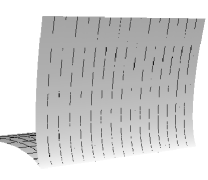
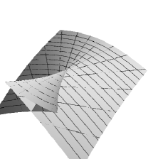
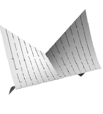
Figure 1. A cuspidal edge, a swallowtail and a cuspidal cross cap.

Fact 1.4 ([11, Proposition 1.3], [3, Corollary 1.5] see also [17, Corollary 2.5]).

Let $f\colon{}\Sigma^{2}\to(M^{3},g)$ be a frontal and $p$ a non-degenerate singular point. Take the singular curve $\gamma(t)$ such that $\gamma(0)=p$ and a null vector field $\eta(t)$ along $\gamma$. Then

1. $f$ at $p$ is a cuspidal edge if and only if $f$ is a front and $\{\gamma^{\prime},\eta\}$ is linearly independent at $p$, that is, $p$ is of the first kind,

2. $f$ at $p$ is a swallowtail if and only if $f$ is a front and $\{\gamma^{\prime},\eta\}$ is linearly dependent at $p$ (i.e., $p$ is of the second kind), but $(d/dt){\operatorname{det}}{}(\gamma^{\prime}(t),\eta(t))|_{t=0}\neq 0$ holds, where ${\operatorname{det}}{}$ denotes an area element of $\Sigma^{2}$, and

3. $f$ at $p$ is a cuspidal cross cap if and only if $\{\gamma^{\prime},\eta\}$ is linearly independent at $p$ (i.e., $p$ is of the first kind), $\psi_{{\operatorname{ccr}}}(0)=0$ and $\psi^{\prime}_{{\operatorname{ccr}}}(0)\neq 0$, where

   $$\psi_{{\operatorname{ccr}}}(t):={\operatorname{det}}{}_{g}\biggl{(}\hat{\gamma}^{\prime}(t),\ \nu\bigl{(}\gamma(t)\bigr{)},\ (\nabla_{\eta}\nu)\bigl{(}\gamma(t)\bigr{)}\biggr{)}\quad\biggl{(}\hat{\gamma}(t):=f\bigl{(}\gamma(t)\bigr{)}\biggr{)},$$

   $\nu$ is the unit normal vector field, and $\nabla$ is the Levi-Civita connection of $(M^{3},g)$.

Regarding $\psi_{{\operatorname{ccr}}}$, the following lemma holds.

Lemma 1.5 ([3, Corollary 1.7]).

Let $f:\Sigma^{2}\to(M^{3},g)$ be a frontal and $p$ a singular point of the first kind. Then $f$ is a front at $p$ if and only if $\psi_{{\operatorname{ccr}}}\neq 0$ at $p$.

Proof.

Since $\eta$ is a null vector and $p$ is a singular point of rank one of $f$, $f$ is a front at $p$ if and only if $\nabla_{\eta}\nu(p)\neq 0$. Thus the necessity is obvious. Let us assume that $\psi_{{\operatorname{ccr}}}=0$ at $p$. Since $p$ is a singular point of the first kind, $\hat{\gamma}^{\prime}\neq 0$ holds at $p$. In particular, $\nabla_{\eta}\nu$ is a linear combination of $\hat{\gamma}^{\prime}$ and $\nu$ at $p$. We now take a local coordinate system $(u,v)$ centered at $p$, such that the $u$-axis is a singular curve, and $v$-directions are null directions along the $u$-axis. Noticing that $\nabla$ is the Levi-Civita connection, it holds that

$$\left\langle{\nabla_{\eta}\nu},{f(\gamma(t))^{\prime}}\right\rangle =\left\langle{\nabla_{\partial_{v}}\nu},{df(\partial_{u})}\right\rangle=(\left\langle{\nu},{f_{u}}\right\rangle)_{v}-\left\langle{\nu},{\nabla_{\partial_{v}}df(\partial_{u})}\right\rangle$$

$$=-\left\langle{\nu},{\nabla_{\partial_{u}}df(\partial_{v})}\right\rangle=-\left\langle{\nu},{df(\partial_{v})}\right\rangle_{u}+\left\langle{\nabla_{\partial_{u}}\nu},{df(\partial_{v})}\right\rangle=0,$$

where $\left\langle{~{}},{~{}}\right\rangle$ is the inner product corresponding to the Riemannian metric $g$, and we used the fact that $df(\partial_{v})=0$ since $\eta=\partial_{v}$ is the null direction. On the other hand, it holds that $\left\langle{\nabla_{\eta}\nu},{\nu}\right\rangle=0$ at $p$. Hence $\nabla_{\eta}\nu(p)=0$ holds. ∎

By Fact 1.4, if $f$ is a front, then a singular point of the first kind gives a cuspidal edge. When $f$ is a frontal but not a front, cuspidal cross caps are typical examples of non-degenerate singular points of the first kind. Swallowtails are singularities of the second kind. Moreover, if $f$ is a front, ‘non-degenerate peaks’ in the sense of [16, Definition 1.10] are also singular points of the second kind.

Example 1.6.

Let $f_{1}\colon{}\boldsymbol{R}^{2}\to\boldsymbol{R}^{3}$ be the map defined by

$$f_{1}(u,v):=(5u^{4}+2uv,v,4u^{5}+u^{2}v-v^{2}).$$

Then the singular set is $\{10u^{3}+v=0\}$, the null vector field is $\eta=\partial_{u}$ and $d\nu(\partial_{u})=(-1,0,0)$ holds at the origin, where $\nu$ is the unit normal vector field. Hence $f_{1}$ is a front and $(0,0)$ is a singular point of the second kind (namely, a non-degenerate peak in the sense of [16, Definition 1.10]) but not a swallowtail (see the left hand side of Fig. 2). On the other hand, let $f_{2}\colon{}\boldsymbol{R}^{2}\to\boldsymbol{R}^{3}$ be the map defined by

$$f_{2}(u,v):=(u^{2}+2v,u^{3}+3uv,u^{5}+5u^{3}v).$$

Then the singular set is $\{v=0\}$, the null vector field is $\eta=\partial_{u}-u\partial_{v}$, and $d\nu(0,0)=(0,0,0)$ holds. Hence $f_{2}$ is a frontal but not a front at the origin $(0,0)$. In fact, $(0,0)$ is a singular point of the second kind (see the right hand side of Fig. 2).

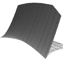
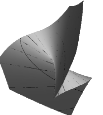
Figure 2. Singularities of the second kind.

Definition 1.7.

Let $p$ be a rank one singular point of a frontal $f\colon{}\Sigma^{2}\to M^{3}$. A local coordinate system $({\mathcal{U}};u,v)$ centered at $p$ is called admissible if $f_{v}(p)=0$ and it is compatible with respect to the orientation of $\Sigma^{2}$.

We denote by ‘$\left\langle{~{}},{~{}}\right\rangle$’ the inner product on $M^{3}$ induced by the metric $g$, and $|{\boldsymbol{a}}|:=\sqrt{\left\langle{{\boldsymbol{a}}},{{\boldsymbol{a}}}\right\rangle}$ (${\boldsymbol{a}}\in TM^{3}$). We fix a unit normal vector field $\nu$ of $f$. Take an admissible coordinate system at a rank one singular point $p$. Then we define

(1.2) $$\kappa_{\nu}(p):=\frac{\left\langle{f_{uu}(p)},{\nu(p)}\right\rangle}{|f_{u}(p)|^{2}},$$

which is called the limiting normal curvature. Here, we denote $f_{uu}:=\nabla_{\partial_{u}}f_{u}$. The definition of $\kappa_{\nu}(p)$ does not depend on the choice of the admissible coordinate system (see Proposition 1.9). Moreover, $\kappa_{\nu}(p)$ does not depend on the choice of the orientation of the source domain, but depends on the co-orientability (i.e., the $\pm$-ambiguity of $\nu$). This definition (1.2) of $\kappa_{\nu}$ is a generalization of the previously defined limiting normal curvature

(1.3) $$\kappa_{\nu}(\gamma(t)):=\frac{\left\langle{\hat{\gamma}^{\prime\prime}(t)},{\nu(\gamma(t))}\right\rangle}{|\hat{\gamma}^{\prime}(t)|^{2}}$$

given in [16], where $\gamma(t)$ is a singular curve parameterizing cuspidal edges and

(1.4) $$\hat{\gamma}:=f\circ\gamma,\qquad\hat{\gamma}^{\prime}:=\frac{d}{dt}\hat{\gamma},\qquad\hat{\gamma}^{\prime\prime}:=\nabla_{\hat{\gamma}^{\prime}}\hat{\gamma}^{\prime}.$$

In fact, the following assertion holds:

Proposition 1.8.

The new definition (1.2) of the limiting normal curvature at $p$ coincides with $\kappa_{\nu}$ given in (1.3) when $p=\gamma(0)$ is a non-degenerate singular point of the first kind.

Proof.

Since $\gamma(t)$ consists of non-degenerate singular points of the first kind for sufficiently small $t$, we can take an admissible coordinate system $(u,v)$ centered at $\gamma(0)$ so that the $u$-axis is a singular curve and $\partial_{v}$ is the null direction. Since $f(u,0)=\hat{\gamma}(u)$, (1.2) is exactly equal to (1.3) at $t=0$. ∎

Proposition 1.9 (The continuity of the limiting normal curvature).

Let $p$ be a rank one singular point of $f$. The definition of $\kappa_{\nu}$ does not depend on the choice of the admissible coordinate system. Moreover, if $p$ is non-degenerate and $\gamma(t)$ is a singular curve such that $\gamma(0)=p$, and if $\gamma(t)$ $(t\neq 0)$ consists of singular points of the first kind, then it holds that

(1.5) $$\kappa_{\nu}(p)\left(=\lim_{t\to 0}\kappa_{\nu}(\gamma(t))\right)=\lim_{t\to 0}\frac{\left\langle{\hat{\gamma}^{\prime\prime}(t)},{\nu(\gamma(t))}\right\rangle}{|\hat{\gamma}^{\prime}(t)|^{2}},$$

where $\hat{\gamma}(t):=f(\gamma(t))$ and $\hat{\gamma}^{\prime\prime}(t):=\nabla_{\hat{\gamma}^{\prime}(t)}\hat{\gamma}^{\prime}(t)$.

Proof.

Let $(U,V)$ be another admissible coordinate system. Then $U_{u}(p)\neq 0$ holds. Moreover,

$$\left\langle{f_{uu}},{\nu}\right\rangle =-\left\langle{f_{u}},{\nu_{u}}\right\rangle=-U_{u}\left\langle{f_{U}},{U_{u}\nu_{U}+V_{u}\nu_{V}}\right\rangle$$

$$=-U_{u}^{2}\left\langle{f_{U}},{\nu_{U}}\right\rangle-U_{u}V_{u}\left\langle{f_{U}},{\nu_{V}}\right\rangle$$

holds at $p$, where $\nu_{u}=\nabla_{\partial_{u}}\nu$, etc. Since

(1.6) $$\left\langle{f_{U}},{\nu_{V}}\right\rangle=-\left\langle{f_{UV}},{\nu}\right\rangle=-\left\langle{f_{VU}},{\nu}\right\rangle=\left\langle{f_{V}},{\nu_{U}}\right\rangle=0$$

at $p$, we have that

$$\frac{\left\langle{f_{uu}},{\nu}\right\rangle}{|f_{u}|^{2}}=-\frac{U_{u}^{2}\left\langle{f_{U}},{\nu_{U}}\right\rangle}{U_{u}^{2}|f_{U}|^{2}}=\frac{\left\langle{f_{UU}},{\nu}\right\rangle}{|f_{U}|^{2}}$$

at $p$, which proves the first assertion. The second assertion follows immediately from (1.3) and Proposition 1.8. ∎

Remark 1.10.

Recently, Nuño-Ballesteros and the first author [12] defined a notion of umbilic curvature $\kappa_{u}$ for rank one singular points in $\boldsymbol{R}^{3}$. We remark that the unsigned limiting normal curvature $\kappa_{n}:=|\kappa_{\nu}|$ coincides with $\kappa_{u}$ for cuspidal edges, see [13] for details.

Example 1.11.

Define a $C^{\infty}$-map $f\colon{}\boldsymbol{R}^{2}\to\boldsymbol{R}^{3}$ by

$$f(u,v)=\left(u^{4}-4u^{2}v,u^{3}-3uv,\frac{u^{2}}{2}-v\right)+(u^{2}-2v)^{2}(a,b,0)\quad(a,b\in\boldsymbol{R}).$$

Then the singular set of $f$ is $\{v=0\}$ and the origin is a swallowtail. The unit normal vector field of $f$ is given by

$$\nu(u,v):=\frac{\big{(}3,-8u,-4(3(-1+a)u^{2}-8bu^{3}-6av+16buv)\big{)}}{\sqrt{9+64u^{2}+16(3(-1+a)u^{2}-8bu^{3}-6av+16buv)^{2}}}.$$

Since $f_{u}(0,0)=0$ holds, by (1.2), the limiting normal curvature at $(0,0)$ is $8a$ (cf. (1.2)). On the other hand, the limiting normal curvature on $\hat{\gamma}(u)=f(u,0)$, $u\neq 0$ is

$$\frac{\left\langle{\hat{\gamma}^{\prime\prime}(u)},{\nu(u,0)}\right\rangle}{|\hat{\gamma}^{\prime}(u)|^{2}}=8a-\frac{64b}{3}u+O(u^{2}),$$

where $O(u^{\alpha})$ ($\alpha>0$) is a term such that $O(u^{\alpha})/|u|^{\alpha}$ is bounded near $u=0$.

Let $f:\Sigma^{2}\to(M^{3},g)$ be a frontal. Suppose that $p$ is of the first kind. Let $\kappa(t)=|\hat{\gamma}^{\prime\prime}(t)|$ be the curvature function of $\hat{\gamma}:=f\circ\gamma$ in $M^{3}$, where $t$ is the arclength parameter of $\hat{\gamma}$. Then $\kappa_{\nu}=\left\langle{\hat{\gamma}^{\prime\prime}(t)},{\nu}\right\rangle$ gives the normal part of $\hat{\gamma}^{\prime\prime}(t)$. On the other hand, we set

(1.7) $$\kappa_{s}(t):={\operatorname{sgn}}(d\lambda(\eta))\,{\operatorname{det}}{}_{g}\biggl{(}\hat{\gamma}^{\prime}(t),\hat{\gamma}^{\prime\prime}(t),\nu(\gamma(t))\biggr{)},$$

which is called the singular curvature, where $\eta(t)$ is a null vector field along $\gamma$ such that $\{\gamma^{\prime},\eta\}$ is compatible with the orientation of $\Sigma^{2}$, and ${\operatorname{sgn}}(d\lambda(\eta))$ is the sign of the function $d\lambda(\eta)$ at $\gamma(t)$. Since $\kappa_{s}$ can be considered as the tangential component of $\hat{\gamma}^{\prime\prime}(t)$, it holds that

(1.8) $$\kappa^{2}=(\kappa_{s})^{2}+(\kappa_{\nu})^{2}.$$

When $p$ is a cuspidal edge, the singular curvature is defined in [16]. In this case, it was shown in [16] that $\kappa_{s}$ depends only on the first fundamental form (namely, it is intrinsic) and we can prove the following assertion as an application of [16].

Fact 1.12.

Let $p$ be a non-degenerate singular point of the first kind of a frontal $f$. If the Gaussian curvature function $K$ is bounded near $p$, then the limiting normal curvature $\kappa_{\nu}$ vanishes at $p$.

Proof.

In the first paragraph of [16, Theorem 3.1], it was stated that the second fundamental form of a front $f$ vanishes at non-degenerate singular points if $K$ is bounded. In fact, the proof there needed only that $f$ is a frontal. By (1.2), $\kappa_{\nu}$ is a coefficient of the second fundamental form, and must vanish. ∎

Fact 1.12 suggests the existence of a new intrinsic invariant related to the behavior of $\kappa_{\nu}$ and the Gaussian curvature. This is our motivation for introducing the ‘product curvature’ in the following section. As a consequence of our following discussions, the converse assertion of Fact 1.12 is obtained in Theorem 2.9. For a non-degenerate singular point $p$ of the first kind, the derivatives of the limiting normal curvature and the singular curvature with respect to the arclength parameter $t$ of $\hat{\gamma}(t):=f\bigl{(}\gamma(t)\bigr{)}$

$$\kappa^{\prime}_{\nu}(p):=\left.\frac{d\kappa_{\nu}(t)}{dt}\right|_{t=0},\quad\kappa^{\prime}_{s}(p):=\left.\frac{d\kappa_{s}(t)}{dt}\right|_{t=0},$$

where $\gamma(t)$ is the singular curve such that $p=\gamma(0)$, are called the derivate limiting normal curvature and the derivate singular curvature, respectively, which will be useful in the following sections.

2. Cuspidal curvature

Let $\sigma(t)$ be a curve in the Euclidean plane $\boldsymbol{R}^{2}$ and suppose that $t=0$ is a $3/2$-cusp. Then the cuspidal curvature of the $3/2$-cusp is given by (cf. [18] and [21])

(2.1) $$\tau:=\frac{{\operatorname{det}}{}(\sigma^{\prime\prime}(0),\sigma^{\prime\prime\prime}(0))}{|\sigma^{\prime\prime}(0)|^{5/2}}.$$

In [21], the following formula was shown

(2.2) $$\tau=2\sqrt{2}\lim_{t\to 0}\sqrt{|s(t)|}\kappa(t),~{}\quad s(t):=\int_{0}^{t}|\sigma^{\prime}(w)|\,dw,$$

where $\kappa(t)$ is the curvature function of $\sigma(t)$.

Let $p$ be a singular point of the first kind of a frontal $f\colon{}\Sigma^{2}\to(M^{3},g)$, and $\gamma(t)$ a singular curve such that $\gamma(0)=p$. Let $\eta$ be a non-vanishing vector field defined on a neighborhood of $p$ such that $\eta$ points in the null direction along $\gamma$, which is called an extended null vector field. We set

$$f_{\eta}:=df(\eta),\quad f_{\eta\eta}:=\nabla_{\eta}f_{\eta},\quad f_{\eta\eta\eta}:=\nabla_{\eta}f_{\eta\eta}.$$

By definition, $f_{\eta}$ vanishes along $\gamma$. Let $(u,v)$ be an admissible coordinate system at $p$. Since $\partial_{u}$ and $\eta$ are linearly independent at $p$, we may consider $\lambda$ in Definition 1.1 as $\lambda={\operatorname{det}}{}_{g}(f_{u},f_{\eta},\nu)$. Since $\lambda=0$ along $\gamma$, the non-degeneracy of $p$ yields that

(2.3) $$0\neq\lambda_{\eta}={\operatorname{det}}{}_{g}{(f_{u},f_{\eta\eta},\nu)},$$

namely, $f_{u}$ and $f_{\eta\eta}$ are linearly independent at the non-degenerate singular point. Define the exterior product $\times_{g}$ so that

$$\left\langle{{\boldsymbol{a}}\times_{g}{\boldsymbol{b}}},{{\boldsymbol{c}}}\right\rangle={\operatorname{det}}{}_{g}({\boldsymbol{a}},{\boldsymbol{b}},{\boldsymbol{c}})$$

holds for each ${\boldsymbol{a}},{\boldsymbol{b}},{\boldsymbol{c}}\in T_{q}M^{3}$ ($q\in M^{3}$). Since the singular points are non-degenerate, the linear map $df:T_{\gamma(t)}\Sigma^{2}\to T_{\hat{\gamma}(t)}M^{3}$ is of rank $1$. Hence $\hat{\gamma}^{\prime}(t)$ is proportional to $f_{u}$, and then $\hat{\gamma}^{\prime}(t)\times_{g}f_{\eta\eta}\bigl{(}\gamma(t)\bigr{)}$ does not vanish, where $\hat{\gamma}(t):=f\circ\gamma(t)$. Then we define the cuspidal curvature for singular points of the first kind as

(2.4) $$\kappa_{c}(t):=\frac{\bigl{|}\hat{\gamma}^{\prime}(t)\bigr{|}^{3/2}\,\,{\operatorname{det}}{}_{g}\biggl{(}\hat{\gamma}^{\prime}(t),f_{\eta\eta}(\gamma(t)),f_{\eta\eta\eta}(\gamma(t))\biggr{)}}{\biggl{|}\hat{\gamma}^{\prime}(t)\times_{g}f_{\eta\eta}(\gamma(t))\biggr{|}^{5/2}},$$

where $\hat{\gamma}=f(\gamma(t))$ and $\eta$ is chosen so that $\{\gamma^{\prime},\eta\}$ consists of a positively oriented frame on $\Sigma^{2}$ along $\gamma$. If $t$ is the arclength parameter of $\hat{\gamma}$, then

$$\kappa^{\prime}_{c}(p):=\left.\frac{d\kappa_{c}(t)}{dt}\right|_{t=0}$$

is called the derivate cuspidal curvature. The two invariants $\kappa_{c},\kappa^{\prime}_{c}$ do not depend on the choice of the unit normal vector $\nu$.

The following assertion gives a geometric meaning of cuspidal curvature.

Proposition 2.1.

Let $f$ be a front in $\boldsymbol{R}^{3}$ and $p$ a cuspidal edge, and let $\gamma(t)$ be the singular curve such that $\gamma(0)=p$. Then the intersection of the image of $f$ and a plane $P$ passing through $f(p)$ perpendicular to $\hat{\gamma}^{\prime}(0)$ consists of a $3/2$-cusp $\sigma$ in $P$. Furthermore, $\kappa_{c}(0)$ coincides with the cuspidal curvature of the plane curve $\sigma$ (cf. (2.1)) at $p$.

Proof.

Without loss of generality, we may assume that $p=(0,0)$ and $f(p)$ is the origin in $\boldsymbol{R}^{3}$. We denote by $\Gamma$ the intersection of the image of $f$ and the plane $P$ as in the statement. Let $(u,v)$ be an admissible coordinate system. Then we have that

$$\Gamma=\biggl{\{}f(u,v)\,;\,\left\langle{f(u,v)},{f_{u}(0,0)}\right\rangle=0\biggr{\}}.$$

Since $f_{u}(0,0)\neq 0$, by applying the implicit function theorem for

$$\left\langle{f(u,v)},{f_{u}(0,0)}\right\rangle=0,$$

there exists a $C^{\infty}$-function $u=u(v)$ ($u(0)=0$) such that

(2.5) $$\left\langle{f\bigl{(}u(v),v\bigr{)}},{f_{u}(0,0)}\right\rangle=0,$$

and

(2.6) $$\sigma(t):=f(u(t),t)$$

gives a parametrization of the set $\Gamma$. Differentiating (2.5), we have that

(2.7) $$\left\langle{u^{\prime}(v)f_{u}(u(v),v)+f_{v}(u(v),v)},{f_{u}(0,0)}\right\rangle=0,$$

where $u^{\prime}:=du/dv$. Since $f_{v}(0,0)=0$, we have that

(2.8) $$u^{\prime}(0)=0.$$

Differentiating (2.7) again, one can get

(2.9) $$u^{\prime\prime}(0)=-\frac{\left\langle{f_{u}(0,0)},{f_{vv}(0,0)}\right\rangle}{\left\langle{f_{u}(0,0)},{f_{u}(0,0)}\right\rangle}.$$

On the other hand, differentiating (2.6), the equation (2.8) yields that

$$\sigma^{\prime}(0) =0,$$

(2.10) $$\sigma^{\prime\prime}(0) =f_{vv}(0,0)+f_{u}(0,0)u^{\prime\prime}(0),$$

$$\sigma^{\prime\prime\prime}(0) =f_{vvv}(0,0)+3f_{uv}(0,0)u^{\prime\prime}(0)+f_{u}(0,0)u^{\prime\prime\prime}(0),$$

which imply that

$${\operatorname{det}}{}\bigl{(}f_{u}(p),\sigma^{\prime\prime}(0),\sigma^{\prime\prime\prime}(0)\bigr{)}={\operatorname{det}}{}\bigl{(}f_{u}(p),f_{vv}(p),f_{vvv}(p)+3f_{uv}(p)u^{\prime\prime}(0)\bigr{)}\\ ={\operatorname{det}}{}(f_{u}(p),f_{vv}(p),f_{vvv}(p))+3u^{\prime\prime}(0){\operatorname{det}}{}(f_{u}(p),f_{vv}(p),f_{uv}(p)).$$

Since $p$ is not a cross cap, ${\operatorname{det}}{}(f_{u}(p),f_{vv}(p),f_{uv}(p))$ vanishes by the well-known Whitney’s criterion for cross caps [25, Page 161 (b)]. Thus, we get the identity

(2.11) $${\operatorname{det}}{}(f_{u}(p),\sigma^{\prime\prime}(0),\sigma^{\prime\prime\prime}(0))={\operatorname{det}}{}(f_{u}(p),f_{vv}(p),f_{vvv}(p)).$$

By (2.10) and (2.9), we have that

(2.12) $$|\sigma^{\prime\prime}(0)|^{2}=\left\langle{f_{vv}(p)},{f_{vv}(p)}\right\rangle-\frac{\left\langle{f_{vv}(p)},{f_{u}(p)}\right\rangle^{2}}{\left\langle{f_{u}(p)},{f_{u}(p)}\right\rangle}=\frac{|f_{u}(p)\times f_{vv}(p)|^{2}}{|f_{u}(p)|^{2}}.$$

By (2.1), (2.4), (2.11) and (2.12), we get the assertion. ∎

Remark 2.2.

In [13], a normal form of a cuspidal edge singular point in $\boldsymbol{R}^{3}$ was given, and its proof can be applied to a given singular point $p$ of the first kind without any modification. So there exist an isometry $T$ of $\boldsymbol{R}^{3}$ and a local coordinate system $(u,v)$ centered at $p$ such that

$$T\circ f(u,v)=\left(u,\frac{a(u)u^{2}+v^{2}}{2},\frac{b_{0}(u)u^{2}+b_{2}(u)uv^{2}}{2}+\frac{b_{3}(u,v)v^{3}}{6}\right),$$

where $a$, $b_{0}$, $b_{2}$ and $b_{3}$ are $C^{\infty}$-functions. It holds that

$$\kappa_{s}(p)=a(0),\quad\kappa_{\nu}(p)=b_{0}(0),\quad\kappa_{c}(p)=b_{3}(0,0).$$

Moreover, we have that

$$\kappa^{\prime}_{s}(p) =b_{0}(0)b_{2}(0)+3a^{\prime}(0),$$

$$\kappa^{\prime}_{\nu}(p) =-a(0)b_{2}(0)+3b^{\prime}_{0}(0),\quad\kappa^{\prime}_{c}(p)=(b_{3})_{u}(0,0).$$

In particular, since $\kappa_{s}$ is intrinsic, so is $\kappa^{\prime}_{s}$, which gives a geometric meaning for the coefficient $a^{\prime}(0)$. On the other hand,

$$k_{t}(p):=b_{2}(0),\qquad k_{i}(p):=3b^{\prime}_{0}(0),$$

are called the cusp-directional torsion and the edge inflectional curvature, which were investigated in [13].

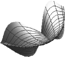
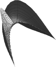
Figure 3. Cuspidal cross caps of $\kappa_{s}>0$ and of $\kappa_{s}<0$.

Example 2.3.

Let $\kappa_{\nu}$, $\kappa_{c}$ and $c$ ($>0$) be constants, and set

$$f(u,v):=\left(u,\frac{\kappa_{s}u^{2}}{2}+\frac{v^{2}}{2},\frac{cuv^{3}}{6}+\frac{\kappa_{\nu}u^{2}}{2}\right).$$

Then the $u$-axis is the singular curve, and $\partial/\partial v$ gives the null direction. A unit normal vector of $f$ is given by

$$\nu:=\frac{1}{\delta}\left(3c\kappa_{s}u^{2}v-cv^{3}-6\kappa_{\nu}u,-3cuv,6\right),$$

where

$$\delta:=\sqrt{9c^{2}u^{2}v^{2}+\left(cv\left(v^{2}-3\kappa_{s}u^{2}\right)+6\kappa_{\nu}u\right)^{2}+36}.$$

By (3) of Fact 1.4, $f(u,v)$ has a cuspidal cross cap singular point at $(0,0)$. The singular curvature and the limiting normal curvature of $f$ at $(0,0)$ are equal to $\kappa_{s}$ and $\kappa_{\nu}$, respectively. Fig. 3 left (resp. right) is the case with $c=6,\kappa_{\nu}=0$ and $\kappa_{s}=2$ (resp. $\kappa_{s}=-2$). The cuspidal curvature along the $u$-axis is

$$\kappa_{c}(u)=\frac{cu\bigl{(}1+\left((\kappa_{\nu})^{2}+(\kappa_{s})^{2}\bigr{)}u^{2}\right)^{3/4}}{(1+(\kappa_{\nu})^{2}u^{2})^{5/4}}.$$

Let $p$ be a point of $\Sigma^{2}$. One can define the ‘blow up’ of the manifold $\Sigma^{2}$ at $p$, that is, there exist a $C^{\infty}$-manifold $\hat{\Sigma}^{2}_{p}$ and consider the blowing up $\Phi:\hat{\Sigma}^{2}_{p}\to\Sigma^{2}$ as in the appendix.

Definition 2.4.

Let ${\mathcal{U}}\,(\subset\Sigma^{2})$ be a neighborhood of $p$, and ${\mathcal{O}}$ an open dense subset of ${\mathcal{U}}$. A real-valued $C^{\infty}$-function $\varphi$ defined on ${\mathcal{O}}$ is called rationally bounded at $p$ if there exists a real-valued $C^{\infty}$-function $\lambda$ defined on $\Phi^{-1}({\mathcal{U}})(\subset\hat{\Sigma}^{2}_{p})$ such that

1. $\Phi^{-1}({\mathcal{O}}\setminus\{p\})=\Phi^{-1}({\mathcal{U}}\setminus\{p\})\cap\lambda^{-1}(\boldsymbol{R}\setminus\{0\})$,

2. $\lambda^{-1}(\{0\})\cap\Phi^{-1}(\{p\})$ is a finite set, and

3. there exists a $C^{\infty}$-function $\psi:\Phi^{-1}({\mathcal{U}})\to\boldsymbol{R}$ such that $\psi(q)=\lambda(q)\,\varphi(\Phi(q))$ holds for $q\in\Phi^{-1}({\mathcal{O}})$.

Moreover, if there exists a constant $c$ such that

(2.13) $$\psi(q)=c\lambda(q)\qquad(q\in\Phi^{-1}(\{p\})),$$

then the function $\varphi$ is called rationally continuous at $p$.

By definition, the continuity implies the rational continuity, and the rational continuity implies the rational boundedness. If $\varphi$ is not continuous but rationally continuous or rationally bounded at $p$, then $p\not\in{\mathcal{O}}$. Let $({\mathcal{U}};u,v)$ be a local coordinate system centered at $p$. We set

$$u:=r\cos\theta,\quad v:=r\sin\theta\qquad(r\geq 0).$$

Suppose that a function $\varphi(u,v)$ is rationally bounded. By definition, there exists a real-valued $C^{\infty}$-function $\lambda$ satisfying (a), (b) and (c). We may consider $\lambda$ the function of two variables $r,\theta$. We denote by $\theta_{1},\dots,\theta_{n}\in[0,2\pi)$ the zeros of the function $\lambda(0,\theta)$. It can be easily checked that for each sufficiently small $\varepsilon>0$, there exist positive constants $\delta,C$ such that the inequality

$$|\varphi(r\cos\theta,r\sin\theta)|<C\qquad(0<r<\delta)$$

holds whenever $|e^{i\theta}-e^{i\theta_{j}}|>\varepsilon$ for each $j=1,\dots,n$, where $i=\sqrt{-1}$. This is a reason why we say that $\varphi$ is rationally bounded. Moreover, if the function $\varphi(u,v)$ is rationally continuous, one can easily check that

$$\lim_{\begin{subarray}{c}(u,v)\to(0,0)\\ (u,v)\in{\mathcal{O}}\end{subarray}}\varphi(u,v)=c$$

holds, where $c$ is the constant as in (2.13). So, we say that $\varphi$ is of rationally continuous.

Example 2.5.

The functions

$$\varphi_{1}(u,v):=1+\frac{uv}{u^{2}-v^{2}},\qquad\varphi_{2}(u,v):=1+\frac{u^{2}v}{u^{2}-v^{2}}$$

are rationally bounded at $(0,0)$ by setting $\lambda(r,\theta):=\cos^{2}\theta-\sin^{2}\theta$. In this case, $\lambda(0,\theta)=0$ if and only if $\theta=(2j+1)\pi/4$ ($j=0,1,2,3$). Moreover, the function $\varphi_{2}$ is rationally continuous at $(0,0)$ by setting $\psi:=\lambda+r\cos^{2}\theta\sin\theta$.

Example 2.6.

For $a\in\boldsymbol{R}\setminus\{0\}$ and $k\geq 2$, we set $f(u,v):=(u,v^{2},v^{3}+au^{k})$. Then its Gaussian curvature function is given by

$$K(u,v)=\frac{3ak(k-1)}{4v}\biggl{(}u^{k-2}+O(1)\biggr{)},$$

where $O(1)$ is a smooth function of $u$ and $v$. Hence $K$ is rationally bounded (resp. rationally continuous) at the origin (with $\lambda(r,\theta)=\sin\theta$) if $k\geq 3$ (resp. $k\geq 4$).

Definition 2.7.

An admissible coordinate system $(u,v)$ (cf. Definition 1.7) at a singular point $p$ of the first kind of a frontal $f$ is called adapted if it is compatible with respect to the orientation of $\Sigma^{2}$, and the following conditions hold along the $u$-axis

1. $|f_{u}|=1$,

2. $f_{v}=0$, in particular, the singular set coincides with the $u$-axis,

3. $\{f_{u},f_{vv},\nu\}$ is an orthonormal frame.

If $(U,V)$ is another adapted coordinate system at $p$, then it holds that

(2.14) $$V_{v}(p)=1.$$

The existence of an adapted coordinate system was shown in [16, Lemma 3.2]. (In fact, the proof of [16, Lemma 3.2] does not use the assumption that $f$ is a front.) Since $\left\langle{f_{vv}},{\nu}\right\rangle=-\left\langle{f_{v}},{\nu_{v}}\right\rangle=0$ along the $u$-axis, (c) is equivalent to the condition that $\left\langle{f_{u}},{f_{vv}}\right\rangle=\left\langle{f_{u}},{f_{v}}\right\rangle_{v}=0$ and $\left\langle{f_{vv}},{f_{vv}}\right\rangle=\frac{1}{2}\left\langle{f_{v}},{f_{v}}\right\rangle_{vv}=1$ along the $u$-axis. Thus, $(u,v)$ is adapted if and only if

(2.15) $$\left\langle{f_{u}},{f_{u}}\right\rangle=1,\qquad\left\langle{f_{v}},{f_{v}}\right\rangle=\left\langle{f_{u}},{f_{v}}\right\rangle_{v}=0,\qquad\left\langle{f_{v}},{f_{v}}\right\rangle_{vv}=2$$

hold along the $u$-axis. In particular, the adapted coordinate system can be characterized in terms of the first fundamental form.

We fix an adapted coordinate system $({\mathcal{U}};u,v)$ of a frontal $f\colon{}\Sigma^{2}\to M^{3}$ such that $\{f_{u},f_{vv},\nu\}$ is a frame compatible with respect to the orientation of $M^{3}$. Then $f_{1}:=f_{u}$ and $f_{2}:=f_{v}/v$ give smooth vector fields on ${\mathcal{U}}$. By definition, $f_{2}(u,0)=f_{vv}(u,0)$. We now set

(2.16) $$\hat{g}_{ij}:=\left\langle{f_{i}},{f_{j}}\right\rangle,\quad\hat{h}_{ij}:=-\left\langle{f_{i}},{\nu_{j}}\right\rangle\qquad(i,j=1,2),$$

where $\nu_{1}:=\nu_{u}$ and $\nu_{2}:=\nu_{v}$. By (a) in Definition 2.7, we have

(2.17) $$\hat{g}_{11}(u,0)=1.$$

On the other hand, we have

(2.18) $$\hat{g}_{12}(u,0)=\left\langle{f_{u}(u,0)},{f_{vv}(u,0)}\right\rangle=0$$

and

(2.19) $$\hat{g}_{22}(u,0)=\lim_{v\to 0}\left\langle{f_{v}(u,v)/v},{f_{v}(u,v)/v}\right\rangle=\left\langle{f_{vv}(u,0)},{f_{vv}(u,0)}\right\rangle=1.$$

Then the mean curvature function $H$ of $f$ is given by

$$H=\frac{\hat{g}_{11}\hat{h}_{22}-2v\hat{g}_{12}\hat{h}_{21}+v\hat{g}_{22}\hat{h}_{11}}{2v(\hat{g}_{11}\hat{g}_{22}-(\hat{g}_{12})^{2})},$$

namely $\hat{H}:=vH$ is a $C^{\infty}$-function of $u,v$ such that $\hat{H}=\frac{1}{2}\hat{h}_{22}+O(v)$, where $O(v)$ is a term such that $O(v)/v$ is bounded near $v=0$. Differentiating $f_{v}=vk$ ($k:=f_{2}$), we have that

$$f_{vv}=k+vk_{v},\quad f_{vvv}=2k_{v}+vk_{vv}.$$

By (c), $\nu=f_{u}\times_{g}f_{vv}$ holds at $(u,0)$. Then we have

(2.20) $$\kappa_{c}={\operatorname{det}}{}_{g}(f_{u},f_{vv},f_{vvv})=\left\langle{\nu},{f_{vvv}}\right\rangle=2\left\langle{\nu},{k_{v}}\right\rangle=-2\left\langle{\nu_{v}},{k}\right\rangle=2\hat{h}_{22}$$

along the $u$-axis. So it holds that

(2.21) $$4\hat{H}(u,0)=\kappa_{c}(u)=\kappa_{c}(p)+\kappa^{\prime}_{c}(p)u+O(u^{2}),$$

which yields the following assertion.

Proposition 2.8.

Let $p$ be a singular point of the first kind of a frontal $f$. Then the mean curvature function $H$ is bounded at $p$ if and only if $\kappa_{c}$ vanishes on a neighborhood of $p$ in the singular set (cf. [16, Corollary 3.5]). Moreover, $H$ is rationally bounded (resp. rationally continuous) at $p$ if and only if $\kappa_{c}(p)=0$ (resp. $\kappa_{c}(p)=\kappa^{\prime}_{c}(p)=0$).

We next discuss the Gaussian curvature $K$ of $f$. The Gaussian curvature $K$ is expressed as

(2.22) $$K=K_{{\operatorname{ext}}}+c_{g}(\nu^{\perp}),$$

where $K_{{\operatorname{ext}}}$ is the extrinsic Gaussian curvature (i.e. the determinant of the shape operator), and $c_{g}(\nu^{\perp})$ is the sectional curvature of the metric $g$ with respect to the $2$-subspace perpendicular to $\nu$ in $T_{f(p)}M^{3}$ (cf. [10, Proposition 4.5]). Since $c_{g}(\nu^{\perp})$ is bounded at $p$, we have that

(2.23) $$K=K_{{\operatorname{ext}}}+O(1)=\frac{\hat{h}_{11}\hat{h}_{22}-v\bigl{(}\hat{h}_{21})^{2}}{v(\hat{g}_{11}\hat{g}_{22}-(\hat{g}_{12})^{2}\bigr{)}}+O(1),$$

where $O(1)$ is a smooth function of $u$ and $v$.

In particular, $\hat{K}:=vK$ is a $C^{\infty}$-function of $u$, $v$. By (a) of Definition 2.7, $u$ is the arclength parameter of the image of the singular curve $\hat{\gamma}(u)=f(u,0)$. Then we have

(2.24) $$\kappa_{\nu}(u)=\left\langle{f_{uu}(u,0)},{\nu(u,0)}\right\rangle=-\left\langle{f_{u}(u,0)},{\nu_{u}(u,0)}\right\rangle=\hat{h}_{11}(u,0).$$

By (2.17), (2.18), (2.19), (2.20), (2.24) and (2.23), we have that

(2.25) $$2\hat{K}(u,0)=\kappa_{\Pi}(u)=\kappa_{\Pi}(p)+\kappa^{\prime}_{\Pi}(p)u+O(u^{2}),$$

where

(2.26) $$\kappa_{\Pi}(u):=\kappa_{\nu}(u)\kappa_{c}(u),\qquad\kappa^{\prime}_{\Pi}(p):=\kappa^{\prime}_{\nu}(p)\kappa_{c}(p)+\kappa_{\nu}(p)\kappa^{\prime}_{c}(p).$$

We call $\kappa_{\Pi}$ and $\kappa^{\prime}_{\Pi}$ the product curvature and the derivate product curvature, respectively. By (a) of Definition 2.7 and (2.14), $\displaystyle\lim_{v\to 0}vK(u,v)$ does not depend on the choice of adapted coordinate system. Since the adapted coordinate system can be characterized in terms of the first fundamental form, we get the following:

Theorem 2.9.

Let $f$ be a frontal and $p$ a singular point of the first kind. Then $\kappa_{\Pi}$ and $\kappa^{\prime}_{\Pi}$ are both intrinsic invariants. Moreover, the Gaussian curvature $K$ is rationally bounded (resp. rationally continuous) at $p$ if and only if $\kappa_{\Pi}=0$ (resp. $\kappa_{\Pi}=\kappa^{\prime}_{\Pi}=0$) holds at $p$. Furthermore, $K$ is bounded on a neighborhood ${\mathcal{U}}$ of $p$ if and only if $\kappa_{\Pi}=0$ along the singular curve in ${\mathcal{U}}$.

Proof.

The rational boundedness (resp. rational continuity) of $K$ can be proved by setting $\lambda=\sin\theta$, since $\hat{K}=vK$ and $v=r\sin\theta$. The last assertion (i.e. the boundedness of $K$ on ${\mathcal{U}}$) is proved as follows: If $K$ is bounded on a neighborhood ${\mathcal{U}}$ of $p$, then $\kappa_{\Pi}$ must vanish identically because of the identity $2\hat{K}(u,0)=\kappa_{\Pi}(u)$ (cf. (2.25)). On the other hand, we suppose $\kappa_{\Pi}(u)=0$ along the $u$-axis. Then by (2.25), $\hat{K}(u,0)=0$ and hence there exists a $C^{\infty}$-function $\varphi(u,v)$ defined on a neighborhood $p$ such that

$$(vK(u,v)=)\hat{K}(u,v)=v\varphi(u,v).$$

Thus the identity $K(u,v)=\varphi(u,v)$ holds whenever $v\neq 0$. This implies that the Gaussian curvature is bounded. ∎

Remark 2.10.

In [16], a necessary and sufficient condition of the boundedness of Gaussian curvature at non-degenerate front singularities is given. However, for singular points on a surface which is frontal but not front, the criterion in [16] does not work. In this sense, the last statement of Theorem 2.9 is a generalization of [16, Theorem 3.1].

By [16, Corollary 3.5], $\kappa_{c}(p)\neq 0$ holds if $p$ is a cuspidal edge. In fact, the following assertion holds.

Proposition 2.11.

Let $f$ be a frontal and $p$ a non-degenerate singular point of the first kind. Then $f$ is a front at $p$ if and only if $\kappa_{c}(p)\neq 0$.

Proof.

On an adapted coordinate system, $\kappa_{c}={\operatorname{det}}{}_{g}(f_{u},f_{vv},f_{vvv})$ holds at $(u,0)$. On the other hand, since $f_{v}(u,0)=0$ holds, $f_{uv}(u,0)=0$. By using the formula

$${\operatorname{det}}{}_{g}({\boldsymbol{x}},{\boldsymbol{a}}\times{\boldsymbol{x}},{\boldsymbol{b}}\times{\boldsymbol{x}})=|{\boldsymbol{x}}|^{2}{\operatorname{det}}{}_{g}({\boldsymbol{x}},{\boldsymbol{a}},{\boldsymbol{b}})\qquad({\boldsymbol{a}},{\boldsymbol{b}},{\boldsymbol{x}}\in T_{o}M^{3},\,\,o\in M^{3}),$$

it holds that

$$\psi_{{\operatorname{ccr}}}(u) ={\operatorname{det}}{}_{g}(f_{u},\nu,\nu_{v})=\left.{\operatorname{det}}{}_{g}(f_{u},f_{u}\times_{g}f_{vv},f_{u}\times_{g}f_{vvv})\right|_{(u,v)=(u,0)}$$

$$=\left.{\operatorname{det}}{}_{g}(f_{u},f_{vv},f_{vvv})\right|_{(u,v)=(u,0)}.$$

Hence the assertion follows from Lemma 1.5. ∎

Proposition 2.11 yields the following:

Corollary 2.12.

Let $p$ be a cuspidal edge. Then $K$ is rationally bounded (resp. rationally continuous) at $p$ if and only if $\kappa_{\nu}=0$ (resp. $\kappa_{\nu}=\kappa^{\prime}_{\nu}=0$) holds at $p$.

Corollary 2.13.

Let $p$ be a singular point of the first kind of a frontal. If the mean curvature $H$ is bounded (resp. rationally bounded, rationally continuous) at $p$, then the Gaussian curvature $K$ is bounded (resp. rationally bounded, rationally continuous) at $p$.

Proof.

The assertion follows from Proposition 2.8, the identity (2.26) and Theorem 2.9. ∎

A singular point $p\in\Sigma^{2}$ of a map $f:\Sigma^{2}\to M^{3}$ is a $5/2$-cuspidal edge if the map germ $f$ at $p$ is right-left equivalent to $(u,v)\mapsto(u,v^{2},v^{5})$ at the origin. The map $f$ is a frontal on a neighborhood of the $5/2$-cuspidal edge $p$, but not a front at $p$.

Corollary 2.14.

Let $p$ be a $5/2$-cuspidal edge. Then the mean curvature $H$ and the Gaussian curvature $K$ are both bounded near $p$.

Proof.

Since singular points on a neighborhood of $p$ consists of $5/2$-cuspidal edges, all singular points are not front singularities. Then the cuspidal curvature $\kappa_{c}$ vanishes identically on the singular set because of Lemma 1.5 and the proof of Proposition 2.11. Thus the boundedness of $H$ and $K$ follow from Proposition 2.8 and Corollary 2.13. ∎

Example 2.15.

A useful criterion for $5/2$-cuspidal edge singularities is given in [9]. Applying this, one can check that the map $f\colon{}\boldsymbol{R}^{2}\to\boldsymbol{R}^{3}$ defined by

$$f(u,v):=(u,au^{2}+v^{2},cu^{2}+bv^{5})$$

has $5/2$-cuspidal edge singularities along the $u$-axis. The unit normal vector field is given by

$$\nu:=\frac{1}{\sqrt{\left(4cu-10abuv^{3}\right)^{2}+25b^{2}v^{6}+4}}\left(10abuv^{3}-4cu,-5bv^{3},2\right).$$

The limiting normal curvature are given by

$$\kappa_{\nu}(u) =\frac{2c}{\sqrt{4c^{2}u^{2}+1}\left(4a^{2}u^{2}+4c^{2}u^{2}+1\right)}.$$

On the other hand, the Gaussian curvature is given by

$$K=-\frac{60bv\left(5abv^{3}-2c\right)}{\left(25b^{2}v^{6}\left(4a^{2}u^{2}+1\right)-80abcu^{2}v^{3}+16c^{2}u^{2}+4\right)^{2}}$$

which is bounded at the singular set as shown in Corollary 2.14. In the case of cuspidal edges, the Gaussian curvature $K$ is bounded if and only if $\kappa_{\nu}$ vanishes identically. However, for this $f$ with $c\neq 0$, $K$ is bounded even if $\kappa_{\nu}\neq 0$.

Remark 2.16.

In [16], it was pointed out that the Gaussian curvature of a front $f$ takes opposite signs on the left and right hand sides of the singular curve if $\kappa_{\nu}\neq 0$. This follows immediately from the formula

$$vK=\frac{1}{2}\kappa_{\Pi}+O(\sqrt{u^{2}+v^{2}}),$$

where $O(\sqrt{u^{2}+v^{2}})$ is the term such that $O(\sqrt{u^{2}+v^{2}})/\sqrt{u^{2}+v^{2}}$ is bounded near $(u,v)=(0,0)$.

By regarding that the tensor fields ${\operatorname{det}}{}_{g}$ and $\left\langle{~{}},{~{}}\right\rangle$ are parallel with respect to the Levi-Civita connection of $(M^{3},g)$, Proposition 2.11 and Fact 1.4 (3) yield that $\kappa_{c}(p)=0$ and $\kappa^{\prime}_{c}(p)\neq 0$ hold if $p$ is a cuspidal cross cap. Then by (2.25) and (2.26), we have

Corollary 2.17.

Let $p$ be a cuspidal cross cap. Then $K$ is rationally bounded at $p$. Moreover it is rationally continuous at $p$ if and only if $\kappa_{\nu}(p)=0$.

The Gaussian curvature of the following cuspidal cross cap is rationally bounded but $\kappa_{\nu}\neq 0$ holds.

Example 2.18.

Let us consider a map $f\colon{}\boldsymbol{R}^{2}\to\boldsymbol{R}^{3}$ defined by

$$f(u,v):=(u,v^{2},uv^{3}+u^{2}).$$

Then

$$\nu(u,v):=\frac{1}{\sqrt{4+4(2u+v^{3})^{2}+9u^{2}v^{2}}}\Big{(}-2(2u+v^{3}),-3uv,2\Big{)}$$

gives a unit normal vector field. By a direct calculation, one can see that $(0,0)$ is a cuspidal cross cap singularity with $\kappa_{\nu}(0,0)=2$, and the Gaussian curvature $K$ is

$$K(u,v)=\frac{12(2u-3v^{3})}{v\Big{(}4+16u^{2}+9u^{2}v^{2}+16uv^{3}+4v^{6}\Big{)}^{2}}.$$

This is rationally bounded at $(0,0)$.

Remark 2.19.

If the ambient space is $\boldsymbol{R}^{3}$, we can take the normal form at a cuspidal edge $p=(0,0)$ as in Remark 2.2. Then the $C^{\infty}$-function $\hat{K}:=vK(u,v)$ satisfies

$$2\hat{K}=\kappa_{\Pi}+\kappa^{\prime}_{\Pi}u-v\left(2(b_{2})^{2}+\frac{\kappa_{s}(\kappa_{c})^{2}}{2}-\frac{8(b_{3})_{v}\kappa_{\nu}}{3}\right)+O(u^{2}+v^{2}),$$

where $O(u^{2}+v^{2})$ is the term such that $O(u^{2}+v^{2})/(u^{2}+v^{2})$ is bounded near $p=(0,0)$. If $K\geq 0$ near $p$, then $\kappa_{\nu}=0$ and thus

$$0\leq 4K(0,0)=-4(b_{2})^{2}-\kappa_{s}(\kappa_{c})^{2}$$

holds. So we have $\kappa_{s}\leq 0$, which reproves the second assertion of [16, Theorem 3.1] in the special case that the ambient space is $\boldsymbol{R}^{3}$.

It is classically known that regular surfaces in $\boldsymbol{R}^{3}$ admit non-trivial isometric deformations, and it might be interesting to consider the existence of such deformations at cuspidal edge singularities: Let $\xi(s)$ ($|s|<1$) be a regular curve on the unit sphere $S^{2}(\subset\boldsymbol{R}^{3})$ and let $a(s)$ ($|s|<1$) be with the arclength parameter $s$, a positive valued function. Then

$$f_{a,\xi}(u,v):=v\xi(u)+\int_{0}^{u}a(s)\xi(s)\,ds$$

gives a developable surface with singularities on the $u$-axis. Moreover, (2.4) yields $\kappa_{c}=-2\mu_{g}/\sqrt{a}$, where $\mu_{g}$ is the geodesic curvature of the spherical curve $\xi$. As pointed out in [8], moving $\xi$ so that $\mu_{g}$ varies, we get an isometric deformation of $f_{a,\xi}$ so that $\kappa_{c}$ changes. Thus $\kappa_{c}$ is not an intrinsic invariant. It should be remarked that we cannot conclude that $\kappa_{\nu}$ is an extrinsic invariant since $f_{a,\xi}$ preserves the limiting normal curvature $\kappa_{\nu}$ to be identically zero. However, using the fact that the product curvature $\kappa_{\Pi}$ is intrinsic (cf. Theorem 2.9), the existence of isometric deformations of cuspidal edges in $\boldsymbol{R}^{3}$ which change $\kappa_{\nu}$ is shown in [14]. See also Teramoto [23] for other geometric properties of cuspidal edges and their parallel surfaces.

3. Singularities of the second kind.

We fix a frontal $f:\Sigma^{2}\to(M^{3},g)$ in an oriented Riemannian $3$-manifold. We consider singular points of the second kind of $f$. Typical such singular points are swallowtails. In this section, we newly define ‘normalized singular curvature’ $\mu_{c}$ and ‘normalized product curvature’ $\mu_{\Pi}$ at singular points of the second kind. Also, ‘limiting singular curvature’ $\tau_{s}$ and ‘limiting cuspidal curvature’ $\tau_{c}$ are defined for swallowtail singularities.

Definition 3.1.

Let $p\in\Sigma^{2}$ be a singular point of the second kind. A local coordinate system $({\mathcal{U}};u,v)$ at $p=(0,0)$ is called adapted at $p$ if it is compatible with respect to the orientation of $\Sigma^{2}$, and the following conditions hold:

1. $f_{u}(p)=0$,

2. the singular set of $f$ on ${\mathcal{U}}$ coincides with the $u$-axis,

3. $|f_{v}(p)|=1$.

The existence of adapted coordinate system can be proved easily. Let $(U,V)$ be another adapted coordinate system, then the condition $f_{u}(p)=0$ and (iii) yield that

(3.1) $$V_{v}(p)=1.$$

We fix an adapted coordinate system $(u,v)$ at $p=(0,0)$. Then one can take a null vector field along the $u$-axis in the form

(3.2) $$\eta=\partial_{u}+\varepsilon(u)\partial_{v}\qquad\bigl{(}\varepsilon(0)=0\bigr{)}$$

for a $C^{\infty}$-function $\varepsilon=\varepsilon(u)$. We can extend this $\eta$ as a vector field defined on a neighborhood of the origin. Since $f_{\eta}=f_{u}+\varepsilon(u)f_{v}$ vanishes on the $u$-axis, there exists a $C^{\infty}$-function $\psi$ such that

(3.3) $$f_{\eta}(u,v)=f_{u}(u,v)+\varepsilon(u)f_{v}(u,v)=v\psi(u,v).$$

Differentiating this by $v$, we have that $\psi(0,0)=f_{uv}(0,0)$. Since $\lambda(u,0)=0$, the non-degeneracy of $p$ yields that

$$0\neq\lambda_{v}={\operatorname{det}}{}_{g}(f_{uv},f_{v},\nu)={\operatorname{det}}{}_{g}(\psi,f_{v},\nu)$$

at $p$, which implies that $\psi(0,0)$ and $f_{v}(0,0)$ are linearly independent. We now set

$$g_{ij}:=\left\langle{f_{u_{i}}},{f_{u_{j}}}\right\rangle,\quad h_{ij}:=-\left\langle{f_{u_{i}}},{\nu_{u_{j}}}\right\rangle\qquad(i,j=1,2),$$

where $u_{1}=u$ and $u_{2}=v$. Since $f_{u}=v\psi-\varepsilon f_{v}$ as in (3.3), it holds that

(3.4) $$g_{11} =\left\langle{v\psi-\varepsilon f_{v}},{v\psi-\varepsilon f_{v}}\right\rangle=v^{2}|\psi|^{2}-2v\varepsilon\left\langle{\psi},{f_{v}}\right\rangle+\varepsilon^{2}|f_{v}|^{2},$$

$$g_{12} =\left\langle{v\psi-\varepsilon f_{v}},{f_{v}}\right\rangle=v\left\langle{\psi},{f_{v}}\right\rangle-\varepsilon|f_{v}|^{2},$$

$$g_{22} =|f_{v}|^{2},$$

which yields that

(3.5) $$g_{11}g_{22}-(g_{12})^{2}=v^{2}(|\psi|^{2}|f_{v}|^{2}-\left\langle{\psi},{f_{v}}\right\rangle^{2})=v^{2}|\psi\times_{g}f_{v}|^{2}.$$

On the other hand,

$$\left\langle{f_{u}+\varepsilon f_{v}},{\nu_{u_{i}}}\right\rangle=\left\langle{f_{\eta}},{\nu_{u_{i}}}\right\rangle=v\left\langle{\psi},{\nu_{u_{i}}}\right\rangle\quad(i=1,2)$$

holds, namely, we have

$$-h_{11}-\varepsilon h_{12}=v\left\langle{\psi},{\nu_{u}}\right\rangle,\quad-h_{12}-\varepsilon h_{22}=v\left\langle{\psi},{\nu_{v}}\right\rangle.$$

So we have that

$$h_{12}=-v\left\langle{\psi},{\nu_{v}}\right\rangle-\varepsilon h_{22},\qquad h_{11}=-v\left\langle{\psi},{\nu_{u}}\right\rangle+v\varepsilon\left\langle{\psi},{\nu_{v}}\right\rangle+\varepsilon^{2}h_{22},$$

and then

$$g_{11}h_{22}-2g_{12}h_{12} +g_{22}h_{11}$$

$$=-v|f_{v}|^{2}\left\langle{\psi},{\nu_{u}+\varepsilon\nu_{v}}\right\rangle+v^{2}\bigl{(}|\psi|^{2}h_{22}+2\left\langle{\psi},{f_{v}}\right\rangle\left\langle{\psi},{\nu_{v}}\right\rangle\bigr{)}$$

$$=-v|f_{v}|^{2}\left\langle{\psi},{\nu_{\eta}}\right\rangle+v^{2}\bigl{(}|\psi|^{2}h_{22}+2\left\langle{\psi},{f_{v}}\right\rangle\left\langle{\psi},{\nu_{v}}\right\rangle\bigr{)}.$$

So by (3.5), the mean curvature $H$ of $f$ is expressed as

$$2vH =v\left(\frac{g_{11}h_{22}-2g_{12}h_{12}+g_{22}h_{11}}{g_{11}g_{22}-(g_{12})^{2}}\right)$$

$$=\frac{-|f_{v}|^{2}\left\langle{\psi},{\nu_{\eta}}\right\rangle+v\bigl{(}|\psi|^{2}h_{22}+2\left\langle{\psi},{f_{v}}\right\rangle\left\langle{\psi},{\nu_{v}}\right\rangle\bigr{)}}{|\psi\times_{g}f_{v}|^{2}}.$$

Then $\hat{H}:=vH$ is a $C^{\infty}$-function of $u$, $v$. We define two constants $\mu_{c}(p)$ and $\mu^{\prime}_{c}(p)$ by the expansion

(3.6) $$2\hat{H}(u,0)=\frac{-|f_{v}(u,0)|^{2}\left\langle{\psi(u,0)},{\nu_{\eta}(u,0)}\right\rangle}{|\psi(u,0)\times_{g}f_{v}(u,0)|^{2}}=\mu_{c}(p)+\mu^{\prime}_{c}(p)u+O(u^{2}).$$

Thus, $H$ is rationally bounded (resp. rationally continuous) at $p$ if and only if $\mu_{c}(p)=0$ (resp. $\mu_{c}(p)=\mu^{\prime}_{c}(p)=0$). By (3.1) and the fact $\hat{H}=vH$, $\mu_{c}(p)$ is a geometric invariant called normalized cuspidal curvature. However, $\mu^{\prime}_{c}(p)$ does depend on the choice of the parameter $u$. Since $|f_{v}(0,0)|=1$, the following formula holds

(3.7) $$\mu_{c}(p)=\frac{-\left\langle{\psi(0,0)},{\nu_{u}(0,0)}\right\rangle}{|\psi(0,0)\times_{g}f_{v}(0,0)|^{2}}=\frac{-\left\langle{f_{uv}(0,0)},{\nu_{u}(0,0)}\right\rangle}{|f_{uv}(0,0)\times_{g}f_{v}(0,0)|^{2}}.$$

The right-hand side of (3.7) is independent of the choice of an adapted coordinate system. Moreover, if we take a positively oriented local coordinate system $(u,v)$ satisfying only (i) of Definition 3.1, then we can write

(3.8) $$\mu_{c}(p)=\frac{-|f_{v}(0,0)|^{3}\left\langle{f_{uv}(0,0)},{\nu_{u}(0,0)}\right\rangle}{|f_{uv}(0,0)\times_{g}f_{v}(0,0)|^{2}},$$

which might be useful rather than (3.7). The invariant $\mu_{c}$ plays a similar role as the cuspidal curvature for non-degenerate singular points of the first kind. For example, the following assertion holds (cf. Proposition 2.11).

Proposition 3.2.

Let $f$ be a frontal and $p$ a non-degenerate singular point of the second kind. Then the following three assertions are equivalent:

1. the mean curvature function is rationally bounded at $p$,

2. $f$ is not a front at $p$,

3. the normalized cuspidal curvature $\mu_{c}$ vanishes at $p$.

Proof.

The equivalency of (1) and (3) has already been mentioned. So it is sufficient to show the equivalency of (2) and (3). Let $(u,v)$ be an adapted coordinate system centered at $p$. Since $p$ is a non-degenerate singular point, the signed area density function (cf. Definition 1.1) satisfies $(\lambda_{u}(p),\lambda_{v}(p))\neq(0,0)$. Since $\lambda_{u}(p)=0$ and $f_{u}(p)=0$, we have

(3.9) $$0\neq\lambda_{v}(p)={\operatorname{det}}{}_{g}(f_{u},f_{v},\nu)_{v}(p)={\operatorname{det}}{}_{g}(f_{uv}(p),f_{v}(p),\nu(p)).$$

On the other hand, since $f_{u}(p)=0$, we have

$$\langle f_{v}(p),\nu_{u}(p)\rangle=-\langle f_{uv}(p),\nu(p)\rangle=\langle f_{u}(p),\nu_{v}(p)\rangle=0.$$

In particular, $f_{v}(p),\nu(p),\nu_{u}(p)$ are mutually orthogonal in $T_{p}M^{3}$. Thus, (3.9) implies that $\langle f_{uv}(p),\nu_{u}(p)\rangle\neq 0$ if and only if $f_{v}$ and $\nu_{u}$ are linearly independent (i.e. $f$ is a front at $p$), proving the assertion. ∎

We set

(3.10) $$\mu_{\Pi}:=\kappa_{\nu}\mu_{c}$$

and call it the normalized product curvature at $p$. We now investigate the relationship between $\mu_{\Pi}$ and the behavior of Gaussian curvature near the singular set. Since the Gaussian curvature $K$ of $f$ satisfies (cf. (2.22))

$$\hat{K}:=vK=v\frac{h_{11}h_{22}-(h_{12})^{2}}{g_{11}g_{22}-(g_{12})^{2}}+O(v),$$

we have the equality

(3.11) $$\hat{K}(u,0) =\left.\frac{-v^{2}\left\langle{\psi},{\nu_{u}}\right\rangle h_{22}-v^{2}\varepsilon\left\langle{\psi},{\nu_{v}}\right\rangle h_{22}-v^{3}\left\langle{\psi},{\nu_{v}}\right\rangle^{2}}{v^{2}|\psi\times_{g}f_{v}|^{2}}\right|_{v=0}$$

$$=\frac{-\left\langle{\psi},{\nu_{\eta}}\right\rangle h_{22}}{|\psi\times_{g}f_{v}|^{2}}=2\hat{H}(u,0)\frac{h_{22}(u,0)}{|f_{v}(u,0)|^{2}}=2\hat{H}(u,0)\kappa_{\nu}(u),$$

here we used the relation $\kappa_{\nu}=h_{22}/|f_{v}|^{2}|_{v=0}$ obtained by (1.5) in Proposition 1.9, where $\kappa_{\nu}(u)$ is the limiting normal curvature defined in Section 1. Then we have

(3.12) $$\hat{K}(u,0) =2\hat{H}(u,0)\biggl{(}\kappa_{\nu}(p)+\hat{\kappa}^{\prime}_{\nu}(p)u+O(u^{2})\biggr{)}$$

$$=\biggl{(}\mu_{c}(p)+\mu^{\prime}_{c}(p)u+O(u^{2})\biggr{)}\biggl{(}\kappa_{\nu}(p)+\hat{\kappa}^{\prime}_{\nu}(p)u+O(u^{2})\biggr{)}$$

$$=\mu_{\Pi}(p)+\biggl{(}\mu_{c}(p)\hat{\kappa}^{\prime}_{\nu}(p)+\mu^{\prime}_{c}(p)\kappa_{\nu}(p)\biggr{)}u+O(u^{2}).$$

We remark that $\hat{\kappa}^{\prime}_{\nu}(p)$ is the derivative of $\kappa_{\nu}(u)$ with respect to the non-arclength parameter $u$. (On the other hand, $\kappa^{\prime}_{\nu}(p)$ in (2.26) is the derivative with respect to the arclength parameter.) Since the notion of adapted coordinate system is described in terms of first fundamental forms, the relation (3.1) implies that $\hat{K}(0,0)$ is an intrinsic invariant. So we get the following

Proposition 3.3.

Let $f\colon{}\Sigma^{2}\to(M^{3},g)$ be a frontal and $p$ a non-degenerate singular point of the second kind. Then the normalized product curvature $\mu_{\Pi}$ (cf. (3.10)) is an intrinsic invariant. Moreover, the Gaussian curvature $K$ is rationally bounded at $p$ if and only if $\mu_{\Pi}(p)=0$.

Since $\hat{\kappa}^{\prime}_{\nu}(p)=d\kappa_{\nu}(u,0)/du|_{u=0}$ depends on the parameter $u$, we consider the co-vector

$$\omega_{\nu}(p):=\hat{\kappa}^{\prime}_{\nu}(p)\,du\in T_{p}^{*}\Sigma^{2}$$

instead, which does not depend on the choice of parameter of the singular curve $\gamma$. By (3.12), we also get the following:

Theorem 3.4.

Let $f\colon{}\Sigma^{2}\to(M^{3},g)$ be a front and $p$ a non-degenerate singular point of the second kind. Then the Gaussian curvature $K$ is rationally bounded (resp. rationally continuous) at $p$ if and only if $\kappa_{\nu}(p)=0$ (resp. $\kappa_{\nu}(p)=0$ and $\omega_{\nu}(p)=0$). Moreover, $K$ is bounded on a neighborhood ${\mathcal{U}}$ of $p$ if and only if $\kappa_{\nu}$ vanishes along the singular curve in ${\mathcal{U}}$.

Proof.

The last assertion (i.e., boundedness of $K$ on ${\mathcal{U}}$) follows from (3.11) by using the same argument of the the last assertion of Theorem 2.9. ∎

Remark 3.5.

Suppose that $p$ is a swallowtail singularity satisfying $\kappa_{\nu}(p)>0$. Let $(u,v)$ be an adapted coordinate system centered at $p$. Then the Gaussian curvature takes different signs on $\{v>0\}$ and $\{v<0\}$ near $p$. We take the unit normal vector field $\nu$ so that the signed area density function $\lambda$ satisfies $\lambda_{v}(p)>0$. A given swallowtail is called positive (resp. negative) if $\lambda_{\eta\eta}>0$ (resp. $\lambda_{\eta\eta}<0$) (cf. [20, Section 3]). Then the domain $\{v<0\}$ (resp. $\{v>0\}$) corresponds to the tail part of the swallowtail (that is, whose image has no self-intersections near $p$, see [16, p. 518]), and so the sign of $-\mu_{\Pi}$ (resp. $\mu_{\Pi}$) coincides with the sign of the Gaussian curvature of the tail part near $p$.

Definition 3.6.

An adapted coordinate system $(u,v)$ at $p$ is called strongly adapted if $f_{uv}$ is perpendicular to $f_{v}$ at $p$.

Lemma 3.7.

For each singular point $p$ of the second kind, there exists a strongly adapted coordinate system.

Proof.

For an adapted coordinate system $(u,v)$, the new coordinate system $(U,V)$ defined by $U:=u$ and $V:=v-\left\langle{f_{uv}(p)},{f_{v}(p)}\right\rangle uv$ gives a strongly adapted coordinate system. ∎

Let $(u,v)$ be a strongly adapted coordinate system at the singular point $p$ of the second kind and take $\psi$ as in (3.3). Since $\left\langle{\psi},{\nu}\right\rangle=\left\langle{f_{u}+\varepsilon f_{v}},{\nu}\right\rangle/v=0$ for $v\neq 0$, the continuity yields that $\psi$ is perpendicular to $\nu$ on the singular set. Moreover, since $\psi(0,0)=f_{uv}(0,0)$ is linearly independent to $f_{v}(0,0)$, $\{f_{v},\psi,\nu\}$ gives a frame field near $(0,0)$. Moreover, $f_{v}\times_{g}\psi$ is proportional to the unit normal vector $\nu$.

Theorem 3.8.

Let $f$ be a frontal and $p$ its singular point of the second kind, and let $\gamma(t)$ be the singular curve such that $\gamma(0)=p$. If $\gamma(t)$ $(t\neq 0)$ is a singular point of the first kind, then it holds that

$$|\mu_{c}(p)|=\lim_{t\to 0}\frac{|\kappa_{c}(\gamma(t))|}{2|\kappa_{s}(\gamma(t))|^{1/2}}.$$

In particular, the product curvature $\kappa_{\Pi}(\gamma(t))$ does not converge to the normalized product curvature $\mu_{\Pi}(p)=\kappa_{\nu}(p)\mu_{c}(p)$.

Proof.

Let $(u,v)$ be a strongly adapted coordinate system and take the null vector field as $\eta=\partial_{u}+\varepsilon(u)\partial_{v}$, where $\varepsilon(u)\neq 0$ for $u\neq 0$ and $\varepsilon(0)=0$. Since $\psi(p)=f_{uv}(p)$ is perpendicular to $f_{v}(p)$, (3.7) reduces to

(3.13) $$\mu_{c}(p)=-\frac{\left\langle{\psi},{\nu_{u}(p)}\right\rangle}{|\psi|^{2}},$$

and by a choice of $\nu$, it holds at $p$ that

(3.14) $$f_{v}\times_{g}\psi=|\psi|\nu.$$

By [16, Page 501], we have that

(3.15) $$\lim_{u\to 0}|\varepsilon(u)\kappa_{s}(u)|=|{\operatorname{det}}{}_{g}(f_{v}(p),f_{uv}(p),\nu)|\\ =|{\operatorname{det}}{}_{g}(f_{v}(p),\psi,\nu)|=|\psi|.$$

On the other hand, we have that

$$f_{\eta\eta}=\psi_{\eta}v+\psi v_{\eta},\quad f_{\eta\eta\eta}=\psi_{\eta\eta}v+2\psi_{\eta}v_{\eta}+\psi v_{\eta\eta}.$$

Since $v_{\eta}=v_{u}+\varepsilon v_{v}=\varepsilon$, we have that

$$f_{\eta\eta}(u,0)=\psi\varepsilon,\quad f_{\eta\eta\eta}(u,0)=2\psi_{\eta}\varepsilon+\psi v_{\eta\eta}.$$

Let $\gamma(u)=(u,0)$ be the singular curve and set

$$\hat{\eta}(u):={\operatorname{sgn}}(\varepsilon(u))\eta={\operatorname{sgn}}(\varepsilon(u))\bigl{(}\partial_{u}+\varepsilon(u)\partial_{v})$$

for $u\neq 0$. Then $\{\gamma^{\prime},\hat{\eta}\}$ is positively oriented for each $u\neq 0$, and so, the definition (2.4) of the cuspidal curvature $\kappa_{c}$ reduces to

$$\kappa_{c} ={\operatorname{sgn}}(\varepsilon)\frac{|f_{u}|^{3/2}{\operatorname{det}}{}_{g}(f_{u},f_{\eta\eta},f_{\eta\eta\eta})}{|f_{u}\times_{g}f_{\eta\eta}|^{5/2}}$$

$$={\operatorname{sgn}}(\varepsilon)\frac{|\varepsilon f_{v}|^{3/2}{\operatorname{det}}{}_{g}(-\varepsilon f_{v},\varepsilon\psi,2\varepsilon\psi_{\eta}+\psi v_{\eta\eta})}{|(\varepsilon f_{v})\times_{g}(\varepsilon\psi)|^{5/2}}$$

$$=\frac{-2|f_{v}|^{3/2}{\operatorname{det}}{}_{g}(f_{v},\psi,\psi_{\eta})}{\sqrt{|\varepsilon|}|f_{v}\times_{g}\psi|^{5/2}}=\frac{-2|f_{v}|^{3/2}\left\langle{f_{v}\times_{g}\psi},{\psi_{\eta}}\right\rangle}{\sqrt{|\varepsilon|}|f_{v}\times_{g}\psi|^{5/2}}.$$

Thus, by (3.15) and (3.14),

$$\lim_{u\to 0}\frac{|\kappa_{c}|}{2|\kappa_{s}|^{1/2}} =\lim_{u\to 0}\left|\frac{|f_{v}|^{3/2}\left\langle{f_{v}\times_{g}\psi},{\psi_{\eta}}\right\rangle}{\sqrt{|\varepsilon\kappa_{s}|}|f_{v}\times_{g}\psi|^{5/2}}\right|$$

$$=\frac{|\left\langle{\nu(p)},{\psi_{u}(p)}\right\rangle|}{|\psi(p)|^{2}}=\frac{|-\left\langle{\nu_{u}(p)},{\psi(p)}\right\rangle|}{|\psi(p)|^{2}}=|\mu_{c}(p)|$$

because $\eta=\partial_{u}$ at $p$, proving the assertion. ∎

We now assume that $p$ is a swallowtail singularity of $f$. We set (cf. (2.2))

$$\tau_{s}:=2\sqrt{2}\lim_{t\to 0}\sqrt{|t|}\,|\kappa_{s}(\gamma(t))|,$$

and call it the limiting singular curvature at $p$, where $t$ is the arclength parameter of $\hat{\gamma}(t)=f\bigl{(}\gamma(t)\bigr{)}$ for $t\neq 0$. By definition, $\tau_{s}$ is an intrinsic invariant. We remark that $\kappa_{s}$ diverges to $-\infty$ at a swallowtail ([16, Corollary 1.14]), and only the absolute value of $\kappa_{s}$ is meaningful. On the other hand, $\varepsilon^{\prime}(0)\neq 0$ by Fact 1.4 (2), where $\varepsilon(u)$ is the function as in (3.2), and ${}^{\prime}=d/du$. By $f_{uu}(p)=-\varepsilon^{\prime}(0)f_{v}(p)$, it holds that

(3.16) $$\hat{\gamma}^{\prime\prime}(0)\neq 0,$$

where $\hat{\gamma}=f\circ\gamma$.

Proposition 3.9.

Let $f:\Sigma^{2}\to(M^{3},g)$ be a front, and $p\in\Sigma^{2}$ a swallowtail singularity and $\gamma(u)$ the singular curve such that $\gamma(0)=p$. Then the following identity holds (cf. (3.16))

(3.17) $$\tau_{s}=\frac{|{\operatorname{det}}{}_{g}\bigl{(}\hat{\gamma}^{\prime\prime}(0),\hat{\gamma}^{\prime\prime\prime}(0),\nu(p)\bigr{)}|}{|\hat{\gamma}^{\prime\prime}(0)|^{5/2}},$$

where ${}^{\prime}=d/du$ and $\hat{\gamma}=f\circ\gamma$.

Proof.

Take a strongly adapted coordinate system $({\mathcal{U}};u,v)$ and let $t=t(u)$ be the arclength parameter of $\hat{\gamma}=f(u,0)$ for $u\neq 0$. Since the tensor fields ${\operatorname{det}}{}_{g}$ and $\left\langle{~{}},{~{}}\right\rangle$ are parallel with respect to the Levi-Civita connection of $(M^{3},g)$, we have

$$\lim_{u\to 0}\frac{{\operatorname{det}}{}_{g}\big{(}\hat{\gamma}^{\prime},\hat{\gamma}^{\prime\prime},\nu(\gamma)\big{)}}{u^{2}} =\lim_{u\to 0}\frac{{\operatorname{det}}{}_{g}\big{(}\hat{\gamma}^{\prime},\hat{\gamma}^{\prime\prime},\nu(\gamma)\big{)}^{\prime\prime}}{2}$$

$$=\lim_{u\to 0}\frac{{\operatorname{det}}{}_{g}\big{(}\hat{\gamma}^{\prime},\hat{\gamma}^{\prime\prime\prime},\nu(\gamma)\big{)}^{\prime}+{\operatorname{det}}{}_{g}\big{(}\hat{\gamma}^{\prime},\hat{\gamma}^{\prime\prime},\nu(\gamma)^{\prime}\big{)}^{\prime}}{2}$$

$$=\frac{{\operatorname{det}}{}_{g}\big{(}\hat{\gamma}^{\prime\prime},\hat{\gamma}^{\prime\prime\prime},\nu(\gamma)\big{)}}{2}\bigg{|}_{u=0},$$

and

(3.18) $$\lim_{u\to 0}\dfrac{\left\langle{\hat{\gamma}^{\prime}},{\hat{\gamma}^{\prime}}\right\rangle}{u^{2}}=\displaystyle\lim_{u\to 0}\dfrac{\left\langle{\hat{\gamma}^{\prime}},{\hat{\gamma}^{\prime}}\right\rangle^{\prime\prime}}{2}\\ =\displaystyle\left\langle{\hat{\gamma}^{\prime\prime}},{\hat{\gamma}^{\prime\prime}}\right\rangle\big{|}_{u=0}.$$

Since

$$|\kappa_{s}(u)|=\frac{|{\operatorname{det}}{}_{g}(\hat{\gamma}^{\prime}(u),\hat{\gamma}^{\prime\prime}(u),\nu(\gamma(u)))|}{|\hat{\gamma}^{\prime}(u)|^{3}},$$

we have

$$\lim_{u\to 0}|u||\kappa_{s}(u)|=\lim_{u\to 0}\dfrac{|{\operatorname{det}}{}_{g}(\hat{\gamma}^{\prime},\hat{\gamma}^{\prime\prime},\nu(\gamma))|}{|u|^{2}}\dfrac{|u|^{3}}{|\hat{\gamma}^{\prime}|^{3}}=\dfrac{|{\operatorname{det}}{}_{g}(\hat{\gamma}^{\prime\prime},\hat{\gamma}^{\prime\prime\prime},\nu(\gamma))|}{2|\hat{\gamma}^{\prime\prime}|^{3}}\bigg{|}_{u=0}.$$

On the other hand,

$$\lim_{u\to 0}\frac{|t(u)|}{u^{2}}=\lim_{u\to 0}\left|\frac{t(u)}{u^{2}}\right|=\lim_{u\to 0}\frac{|\hat{\gamma}^{\prime}(u)|}{2|u|}=\lim_{u\to 0}\frac{1}{2}\sqrt{\frac{\left\langle{\hat{\gamma}^{\prime}(u)},{\hat{\gamma}^{\prime}(u)}\right\rangle}{u^{2}}}=\frac{|\hat{\gamma}^{\prime\prime}(0)|}{2}$$

holds because of (3.18). Thus we have

(3.19) $$\lim_{u\to 0}\frac{\sqrt{|t(u)|}}{|u|}=\frac{\sqrt{|\hat{\gamma}^{\prime\prime}(0)|}}{\sqrt{2}}.$$

Hence

$$2 \sqrt{2}\lim_{t\to 0}\sqrt{|t|}|\kappa_{s}(t)|=2\sqrt{2}\lim_{u\to 0}\bigg{|}\frac{{\operatorname{det}}{}_{g}\bigl{(}\hat{\gamma}^{\prime},\hat{\gamma}^{\prime\prime},\nu(\gamma)\bigr{)}}{u^{2}}\,\frac{\sqrt{|t(u)|}}{u}\,\frac{u^{3}}{|\hat{\gamma}^{\prime}|^{3}}\bigg{|}$$

$$=2\sqrt{2}\frac{|{\operatorname{det}}{}_{g}(\hat{\gamma}^{\prime\prime},\hat{\gamma}^{\prime\prime\prime},\nu(\gamma))|}{2}\,\frac{\sqrt{|\hat{\gamma}^{\prime\prime}|}}{\sqrt{2}}\,\frac{1}{|\hat{\gamma}^{\prime\prime}|^{3}}\bigg{|}_{u=0}=\frac{|{\operatorname{det}}{}_{g}(\hat{\gamma}^{\prime\prime},\hat{\gamma}^{\prime\prime\prime},\nu(\gamma))|}{|\hat{\gamma}^{\prime\prime}|^{5/2}}\bigg{|}_{u=0}$$

proves the assertion. ∎

Corollary 3.10.

Let $f:\Sigma^{2}\to\boldsymbol{R}^{3}$ be a front, and $p\in\Sigma^{2}$ a swallowtail singularity. Let $P$ be the tangential plane of $f$ at $f(p)$ (that is, the plane passing through $f(p)$ which is orthogonal to $\nu(p)$), and $\sigma$ the orthogonal projection of $\hat{\gamma}:=f\circ\gamma$ to the plane $P$. Then $\tau_{s}$ coincides with the absolute value of the cuspidal curvature of the curve $\sigma$ in the plane $P$.

Proof.

By taking a strongly adapted coordinate system $({\mathcal{U}};u,v)$, it holds that $\sigma(u)=\hat{\gamma}(u)-\left\langle{\hat{\gamma}(u)},{\nu(p)}\right\rangle\nu(p)$. Since $|\nu(p)|=1$, the absolute value of cuspidal curvature of $\sigma$ is equal to

$$\left|\frac{{\operatorname{det}}{}\big{(}\hat{\gamma}^{\prime\prime}(0),\hat{\gamma}^{\prime\prime\prime}(0),\nu(p)\big{)}}{|\sigma^{\prime\prime}(0)|^{5/2}}\right|.$$

Since $\hat{\gamma}^{\prime\prime}(u)=f_{uu}(u,0)$ and $f_{u}(p)=0$, we have

$$\left\langle{f_{uu}(p)},{\nu(p)}\right\rangle=-\left\langle{f_{u}(p)},{\nu_{u}(p)}\right\rangle=0.$$

Thus $|\sigma^{\prime\prime}(p)|=|\hat{\gamma}^{\prime\prime}(p)|$ holds. Hence we have the assertion. ∎

We next consider the limit

$$\tau_{c}:=\frac{\sqrt{2\sqrt{2}}}{2}\lim_{t\to 0}\left||t|^{1/4}\kappa_{c}(\gamma(t))\right|,$$

where $t$ is the arclength parameter of $\hat{\gamma}$. We call $\tau_{c}$ the limiting cuspidal curvature.

Proposition 3.11.

If $f$ is a front and $p$ is a swallowtail, then it holds that

(3.20) $$\tau_{c}=\sqrt{|\tau_{s}|}|\mu_{c}(p)|.$$

Moreover, the following identity holds:

(3.21) $$(\sqrt{|\tau_{s}|}\hat{K}(p)=)\sqrt{|\tau_{s}|}\kappa_{\nu}(p)\mu_{c}(p)={\operatorname{sgn}}(\mu_{c}(p))\kappa_{\nu}(p)\tau_{c}.$$

In particular, the absolute value of the right hand side is intrinsic.

Proof.

Using Theorem 3.8 and Proposition 3.9, we get (3.20). By the definition of $\tau_{c}$, (3.6) and (3.11), we have

$${\operatorname{sgn}}(\mu_{c}(p))\kappa_{\nu}(p)\tau_{c}=\sqrt{|\tau_{s}|}\kappa_{\nu}(p)\mu_{c}(p)=2\sqrt{|\tau_{s}|}\kappa_{\nu}(p)\hat{H}(p)=\sqrt{|\tau_{s}|}\hat{K}(p),$$

which proves the assertion. ∎

Example 3.12.

Consider a front

$$f(u,v):=\left(v+\frac{u^{2}}{2}-\frac{b^{2}u^{2}v}{2}-\frac{b^{2}u^{4}}{8},\ \frac{bu^{3}}{3}+buv,\ \frac{cv^{2}}{2}\right)\qquad(b,c>0)$$

in $\boldsymbol{R}^{3}$, where $\nu:=\bigl{(}2bc\left(u^{2}+v\right),cu\left(b^{2}\left(u^{2}+2v\right)-2\right),-b\left(b^{2}u^{2}+2\right)\bigr{)}/\delta$ and

$$\delta:=\sqrt{b^{6}u^{4}+b^{4}u^{2}\left(c^{2}\left(u^{2}+2v\right)^{2}+4\right)+4b^{2}\left(c^{2}v^{2}+1\right)+4c^{2}u^{2}}.$$

The $u$-axis consists of the singular set of $f$, and $\eta=\partial_{u}-u\partial_{v}$ gives a null vector field of $f$ on the $u$-axis. Thus the origin $(0,0)$ is a swallowtail. Other singular points are cuspidal edges. We have

(3.22) $$2\hat{H}(u,0)=\frac{c}{b^{2}}+O(u^{2}),\qquad\hat{K}(u,0)=-\frac{c^{2}}{b^{2}}+O(u^{2}).$$

On the other hand, we see that

(3.23) $$\kappa_{\nu}(u) =\dfrac{\left\langle{f_{vv}},{\nu}\right\rangle}{|f_{v}|^{2}}=-c+O(u^{2}),$$

(3.24) $$\kappa_{s}(u) =\dfrac{{\operatorname{det}}{}(f_{u},f_{uu},\nu)}{|f_{u}|^{3}}=-\dfrac{b}{u}+O(u),$$

(3.25) $$|\kappa_{c}(u)| =\dfrac{|f_{u}|^{3/2}\left|{\operatorname{det}}{}(f_{u},f_{\eta\eta},f_{\eta\eta\eta})\right|}{|f_{u}\times f_{\eta\eta}|^{5/2}}=\dfrac{2c}{b^{3/2}\sqrt{|u|}}+O(u^{3/2}).$$

Since $(u,v)$ is an adapted coordinate system, using (3.7), we have

(3.26) $$\mu_{c}(0)=c/b^{2}.$$

In particular, the constant term of $\hat{K}$ (cf. (3.22)) is equal to the normalized product curvature

$$\mu_{\Pi}(0)=\kappa_{\nu}(0)\mu_{c}(0)=-c^{2}/b^{2}.$$

On the other hand, by (3.24) and (3.25), we see that

$$\lim_{u\to 0}\dfrac{|\kappa_{c}(u)|}{2|\kappa_{s}(u)|^{1/2}}=\lim_{u\to 0}\dfrac{2c/(b^{3/2}\sqrt{|u|})}{2\left|{b}/{u}\right|^{1/2}}=\dfrac{c}{b^{2}},$$

which coincides with $|\mu_{c}(0)|$ (cf. Theorem 3.8). We set

$$t(u):=\int_{0}^{u}|f_{u}(w,0)|dw,$$

then $t$ gives the arclength parameter of the image of the singular curve. By (3.19) and (3.24), we have that

$$\tau_{s}=2\sqrt{2}\lim_{u\to 0}\sqrt{|t(u)|}|\kappa_{s}(u)|=2\lim_{u\to 0}|u\kappa_{s}(u)|=2b.$$

On the other hand, we have that

$$\left.\frac{{\operatorname{det}}{}(f_{uu},f_{uuu},\nu)}{|f_{uu}|^{5/2}}\right|_{(u,v)=(0,0)}=2b,$$

which verifies the formula (3.17). We next see that

$$\tau_{c}=\frac{\sqrt{2\sqrt{2}}}{2}\lim_{t\to 0}\left||t|^{1/4}\kappa_{c}(\gamma(t))\right|=\frac{\sqrt{2\sqrt{2}}}{2}\lim_{u\to 0}\left|\dfrac{|u|^{1/2}}{2^{1/4}}\dfrac{2c}{b^{3/2}\sqrt{|u|}}\right|=\sqrt{2}\dfrac{c}{b^{3/2}}.$$

On the other hand, we have $\sqrt{|\tau_{s}|}|\mu_{c}(0)|=\sqrt{2}c/{b^{3/2}}$, which verifies (3.20). We also see that $\sqrt{|\tau_{s}|}\hat{K}(0,0)=-\sqrt{2}c^{2}/b^{3/2}$, and $\kappa_{\nu}(0)\tau_{c}=-\sqrt{2}c^{2}/b^{3/2}$, verifying (3.21). Finally, the signed area density function $\lambda$ (cf. Definition 1.1) satisfies $\lambda_{v}(0,0)=b~{}(>0)$. By a straightforward calculation, we have

$$\lambda_{\eta} =-\frac{u}{2d}\biggl{(}b^{6}\left(u^{4}-2u^{2}v\right)+b^{4}\left(u^{2}-v\right)\left(c^{2}\left(u^{2}+2v\right)^{2}+4\right)$$

$$\phantom{aaaaaaaaaaaaaaaaaaaaaaaaaaaaaaa}+b^{2}\left(8c^{2}v^{2}+4\right)+4c^{2}\left(u^{2}-v\right)\biggr{)}$$

and

$$\lambda_{\eta\eta}(0,0)=\left.\frac{\partial\lambda_{\eta}}{\partial u}\right|_{(u,v)=(0,0)}=-b~{}(<0).$$

Thus $(0,0)$ is a negative swallowtail and the tail part is $\{v>0\}$ (cf. Remark 3.5). In particular, the sign of the Gaussian curvature of the tail part coincides with that of $\mu_{\Pi}(0)=-c^{2}/b^{2}$, namely, it is negative valued on the tail part near $(0,0)$ (cf. Fig. 4).

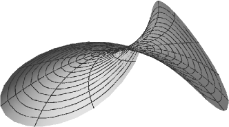
Figure 4. The swallowtail of Example 3.12 with $a=b=1$.

Example 3.13 (Cones of revolution).

Let $\gamma(v)=(x(v),z(v))$ ($|v|<\varepsilon$) be a smooth regular plane curve with arclength parameter such that $x(v)=0$ if and only if $v=0$, where $\varepsilon>0$. We set

$$f(u,v):=(x(v)\cos u,x(v)\sin u,z(v)),\qquad(u,v)\in\boldsymbol{R}/(2\pi\mathbf{Z})\times(-\varepsilon,\varepsilon).$$

Then $\nu(u,v):=(-z^{\prime}(v)\cos u,-z^{\prime}(v)\sin u,x^{\prime}(v))$ gives a unit normal vector field of $f$. The singular set of $f$ is $\{v=0\}$, and its image is a point, so called a cone-like singularity. Since the signed area density function is given by $\lambda(u,v)=-x(v)$, each singular point is non-degenerate if and only if $x^{\prime}(0)\neq 0$. Since the null vector field of $f$ is $\partial_{u}$, the singular points $(u,0)$ are all of the second kind. Moreover, $f$ is a front at $(u,0)$ if and only if $\nu_{u}\neq 0$, that is, $z^{\prime}(0)\neq 0$. So we now assume $x^{\prime}(0)z^{\prime}(0)\neq 0$. The limiting normal curvature of $f$ at $(u,0)$ is $(\kappa_{\nu}:=)-x^{\prime\prime}(0)/z^{\prime}(0)$, which coincides with the curvature of $\gamma(t)$ at $t=0$. In particular, the Gaussian curvature $K$ of $f$ is unbounded if $t=0$ is not an inflection point of $\gamma$. In fact, $K(u,v)=-x^{\prime\prime}(v)/x(v)$ diverges and changes sign at $v=0$ when $\kappa_{\nu}\neq 0$, which verifies the third assertion of Theorem A.

On the other hand, the normalized cuspidal curvature of $f$ is given by $(\mu_{c}:=)z^{\prime}(0)/x^{\prime}(0)$, which does not vanish. In fact,

$$H(u,v)=\frac{1}{2}\left(\frac{z^{\prime}(v)}{x(v)}-\frac{z^{\prime\prime}(v)}{x^{\prime}(v)}\right)$$

diverges at $v=0$, which verifies Proposition 3.2.

We now remark that Theorem B in the introduction follows immediately from Corollary 2.12 and Theorem 3.4. Finally, we prove the Theorem A in the introduction.

(Proof of Theorem A).

Let $f\colon{}{\mathcal{U}}\to(M^{3},g)$ be a front and $p\in{\mathcal{U}}$ a non-degenerate singular point of it. Then $p$ is either of the first kind or of the second kind. Each of these two cases, we can take an adapted coordinate system $(u,v)$ centered at $p$. Then the signed area density function $\lambda(u,v)$ (cf. Definition 1.1) vanishes along the $u$-axis. So we can write $\lambda(u,v)=v\hat{\lambda}(u,v)$, where $\hat{\lambda}(u,v)$ is a smooth function defined on a sufficiently small neighborhood of the $u$-axis, and can write

(3.27) $$K\,d\hat{A}=K\lambda du\wedge dv=\hat{K}\hat{\lambda}\,du\wedge dv,$$

where $\hat{K}:=vK$ and $K$ is the Gaussian curvature of $f$. As in the proofs of Theorems 2.9 and 3.4, $\hat{K}$ is a smooth function on a sufficiently small neighborhood of the $u$-axis, which proves the first assertion. Moreover, $K\,d\hat{A}$ is equal to zero only at a point where $\kappa_{\nu}=0$. So we get the equivalency of (1) and (2).

We next suppose that $\kappa_{\nu}(p)\neq 0$. By the equivalency of (1) and (2), the equality (3.27) yields that $\lim_{v\to 0}K(u,v)\lambda(u,v)\neq 0$. Since $\lambda(u,v)$ changes sign across the $u$-axis, we can conclude that $K$ is unbounded and changes sign between two sides of the $u$-axis.

Finally, we consider the case that $(M^{3},g)$ is the Euclidean 3-space. Since $K\,d\hat{A}$ coincides with the pull-back of the area element of the unit sphere by $\nu$, as pointed out in Remark 1.2, (2) is also equivalent to the fact that $p$ is the singular point of $\nu$. ∎

We denote by $S^{3}$ the unit 3-sphere in $\boldsymbol{R}^{4}$ centered at the origin. For a given front $f:\Sigma^{2}\to S^{3}$, its unit normal vector field $\nu$ can be considered as a map $\nu:\Sigma^{2}\to S^{3}$ using the parallel translations in $\boldsymbol{R}^{4}$. We call this the Gauss map of $f$. As a corollary of Theorem A, we get the following:

Proposition 3.14.

Let $f:\Sigma^{2}\to S^{3}$ be a front, and $p\in\Sigma^{2}$ a non-degenerate singular point. Then the Gauss map $\nu:\Sigma^{2}\to S^{3}$ of $f$ has a singularity at $p$ if and only if the limiting normal curvature $\kappa_{\nu}(p)$ is equal to zero.

Proof.

Since $S^{3}\subset\boldsymbol{R}^{4}$, the signed area element of $f$ is written by

$$d\hat{A}_{f}={\operatorname{det}}{}(f,f_{u},f_{v},\nu),$$

where ‘${\operatorname{det}}{}$’ is the determinant function on $\boldsymbol{R}^{4}$. By using the similar argument as in Remark 1.2, the Weingarten formula and the Gauss equation $K=1+{\operatorname{det}}{}(W)$ yield that

$$d\hat{A}_{\nu}={\operatorname{det}}{}(\nu,\nu_{u},\nu_{v},-f)={\operatorname{det}}{}(W)d\hat{A}_{f}=(K-1)d\hat{A}_{f},$$

where we took $-f$ as the unit normal vector of $\nu$. Since $d\hat{A}_{f}$ vanishes at $p$, the equality $d\hat{A}_{\nu}=(K-1)d\hat{A}_{f}=K\,d\hat{A}_{f}$ holds at $p$. Then the assertion follows from Theorem A and the fact that $d\hat{A}_{\nu}$ vanishes at $p$ if and only if $p$ is a singular point of $\nu$. ∎

The hyperbolic space

$$H^{3}:=\biggl{\{}(t,x,y,z)\in\boldsymbol{R}^{4}_{1}\,;\,t^{2}-x^{2}-y^{2}-z^{2}=1,\,\,t>0\biggr{\}}$$

of constant curvature $-1$ is a hyperboloid in the Lorentz-Minkowski $4$-space $\boldsymbol{R}^{4}_{1}$ with signature $(-,+,+,+)$. Like as in the case of $S^{3}$, for an arbitrarily given front $f:\Sigma^{2}\to H^{3}$, its unit normal vector field can be considered as the Gauss map $\nu:\Sigma^{2}\to S^{3}_{1}$, where

$$S^{3}_{1}:=\biggl{\{}(t,x,y,z)\in\boldsymbol{R}^{4}_{1}\,;\,t^{2}-x^{2}-y^{2}-z^{2}=-1\biggr{\}}$$

is the de Sitter $3$-space. If the Gauss map $\nu:\Sigma^{2}\to S^{3}_{1}$ of $f$ is an immersion, then it is space-like. We also get the following:

Proposition 3.15.

Let $f:\Sigma^{2}\to H^{3}$ be a front, and $p\in\Sigma^{2}$ a non-degenerate singular point. Then the Gauss map $\nu:\Sigma^{2}\to S^{3}_{1}$ of $f$ has a singularity at $p$ if and only if the limiting normal curvature $\kappa_{\nu}(p)$ vanishes.

Appendix: The coordinate invariance of blow up

We give here the procedure of blowing up and show its coordinate invariance, which is used to define rational boundedness and continuity in Definition 2.4.

We define the equivalence relation $\sim$ on $\boldsymbol{R}\times S^{1}$ by

$$(r,\theta)\sim(-r,\theta+\pi),$$

where $S^{1}:=\boldsymbol{R}/2\pi\mathbf{Z}$. We set ${\mathcal{M}}:=\boldsymbol{R}\times S^{1}/\sim$, namely, ${\mathcal{M}}$ is the quotient space of $\boldsymbol{R}\times S^{1}$ by this equivalence relation. We also denote by

$$\pi:\boldsymbol{R}\times S^{1}\to{\mathcal{M}}$$

the canonical projection. Let $(\boldsymbol{R}^{2};u,v)$ be the $(u,v)$-plane. Then there exists a unique $C^{\infty}$-map $\Phi:{\mathcal{M}}\to\boldsymbol{R}^{2}$ such that

$$\Phi\circ\pi(r,\theta):=(r\cos\theta,r\sin\theta)\qquad((r,\theta)\in\boldsymbol{R}\times S^{1}).$$

This map $\Phi$ gives the usual blow up of $\boldsymbol{R}^{2}$ at the origin.

From now on, we show that the coordinate invariance of this blow up procedure: let $(\boldsymbol{R}^{2};U,V)$ be the $(U,V)$-plane, and consider a diffeomorphism $f:(\boldsymbol{R}^{2};u,v)\to(\boldsymbol{R}^{2};U,V)$ such that $f(0,0)=(0,0)$. Then we can write

$$f\circ\Phi\circ\pi(r,\theta)=(U(r,\theta),V(r,\theta)).$$

Since $f(0,0)=(0,0)$, it holds that $U(0,\theta)=V(0,\theta)=0$. Then the well-known division property of $C^{\infty}$-functions yields that there exist $C^{\infty}$-function germs $\xi(r,\theta)$ and $\eta(r,\theta)$ such that

$$U(r,\theta)=r\xi(r,\theta),\qquad V(r,\theta)=r\eta(r,\theta).$$

Since $f$ is a diffeomorphism, one can easily show that $\xi(0,\theta)^{2}+\eta(0,\theta)^{2}$ is positive for all $\theta\in S^{1}$, and the $C^{\infty}$-function

$$R(r,\theta):=r\sqrt{\xi(r,\theta)^{2}+\eta(r,\theta)^{2}}$$

is defined on $\Omega:=(f\circ\Phi\circ\pi)^{-1}\bigl{(}\{(U,V)\,;\,U^{2}+V^{2}<\varepsilon^{2}\}\bigr{)}$ for sufficiently small $\varepsilon>0$. Moreover, there exists a unique $C^{\infty}$-function $\Theta:\Omega\to S^{1}$ such that

$$\cos\Theta(r,\theta)=\frac{\xi(r,\theta)}{\sqrt{\xi(r,\theta)^{2}+\eta(r,\theta)^{2}}},\quad\sin\Theta(r,\theta)=\frac{\eta(r,\theta)}{\sqrt{\xi(r,\theta)^{2}+\eta(r,\theta)^{2}}}.$$

Then, the $C^{\infty}$-map $F:\pi(\Omega)\to\Phi^{-1}(\{(U,V)\,;\,U^{2}+V^{2}<\varepsilon^{2}\})$ satisfying the property $F\circ\pi(r,\theta)=\pi(R(r,\theta),\Theta(r,\theta))$ is uniquely determined, and satisfies the relation $F\circ\Phi=\Phi\circ f$. By our construction, such a map $F$ depends only on $f$. Hence, by replacing $f$ by $f^{-1}$, we can conclude that $F$ is a diffeomorphism for sufficiently small $\varepsilon>0$.

Let $p$ be a point on a $2$-manifold $\Sigma^{2}$. The above construction of $F$ implies that we can define the ‘blow up’ of the manifold $\Sigma^{2}$ at $p$.

Acknowledgements.

The authors thank the referees for careful reading and valuable comments. The third and the fourth authors thank Toshizumi Fukui for fruitful discussions at Saitama University. By his suggestion, we obtained the new definition of rational boundedness and continuity. The second author thanks Shyuichi Izumiya for fruitful discussions.

References

[1]
J. W. Bruce and
J. M. West,
Functions on a crosscap,
Math. Proc. Camb. Phil. Soc. 123
(1998), 19–39.
[2]
F. S. Dias and F. Tari,
On the geometry of the cross-cap
in the Minkowski -space, preprint, 2012,
to appear in Tohoku Mathematical Journal.
Available from
www.icmc.usp.br/~faridtari/Papers/DiasTari.pdf.
[3]
S. Fujimori, K. Saji, M. Umehara and K. Yamada,
Singularities of maximal surfaces,
Math. Z. 259 (2008), 827–848.
[4]
T. Fukui and M. Hasegawa,
Fronts of Whitney umbrella—a differential
geometric approach via blowing up,
J. Singul. 4 (2012), 35–67.
[5]
T. Fukui and M. Hasegawa,
Height functions on Whitney umbrellas,
RIMS Kôkyûroku Bessatsu 38 (2013), 153-168.
[6]
R. Garcia, C. Gutierrez and J. Sotomayor,
Lines of principal curvature around umbilics and Whitney
umbrellas,
Tohoku Math. J. 52 (2000), 163–172.
[7]
M. Hasegawa,
A. Honda, K. Naokawa, K. Saji, M. Umehara and
K. Yamada,
Intrinsic properties of singularities of surfaces,
Internat. J. of Math. 26 (2015), 34pp.
[8]
M. Hasegawa, A. Honda, K. Naokawa, M. Umehara and K. Yamada,
Intrinsic invariants of cross caps,
Selecta Math. 20 (2014), 769–785.
[9]
A. Honda, M. Koiso and K. Saji,
Fold singularities on spacelike CMC surfaces
in Lorentz-Minkowski space, preprint,
arXiv:1509.03050.
[10]
S. Kobayashi and K. Nomizu,
Foundations of
Differential Geometry, Volume 2, John Wiley & Sons, Inc.
(1969).
[11]
M. Kokubu, W. Rossman, K. Saji, M. Umehara and K. Yamada,
Singularities of flat fronts in hyperbolic -space,
Pacific J. Math. 221 (2005), 303–351.
[12]
L. F. Martins and J. J. Nuño-Ballesteros,
Contact properties of surfaces in with corank
singularities,
Tohoku Math. J. 67 (2015), 105–124.
[13]
L. F. Martins and K. Saji,
Geometric invariants of cuspidal edges,
to appear in Canadian Journal of Mathematics, arXiv:1412.4099.
[14]
K. Naokawa, M. Umehara and K. Yamada,
Isometric deformations of cuspidal edges,
to appear in Tohoku Mathematical Journal, arXiv:1408.4243.
[15]
R. Oset Sinha and F. Tari,
Projections of surfaces in
to and the geometry of their singular images,
Rev. Mat. Iberoam. 31 (2015), pp. 33–50.
[16]
K. Saji, M. Umehara and K. Yamada,
The geometry of fronts,
Ann. of Math. 169 (2009), 491–529.
[17]
K. Saji, M. Umehara and K. Yamada,
singularities of wave fronts,
Math. Proc. Camb. Phil. Soc. 146 (2009), 731–746.
[18]
K. Saji, M. Umehara and K. Yamada,
The duality between singular points and
inflection points on wave fronts,
Osaka J. Math. 47 (2010), 591–607.
[19]
K. Saji, M. Umehara and K. Yamada,
Coherent tangent bundles and Gauss-Bonnet
formulas for wave fronts,
J. Geom. Anal.
22 (2012), 383–409.
[20]
K. Saji, M. Umehara and K. Yamada,
An index formula for a bundle homomorphism of
the tangent bundle into a vector bundle of the same rank
and its applications, to appear in the Journal of
Mathematical Society of Japan, arXiv:1202.3854.
[21]
S. Shiba and M. Umehara,
The behavior of curvature functions at cusps and
inflection points,
Diff. Geom. Appl. 30 (2012), 285–299.
[22]
F. Tari,
On pairs of geometric foliations on a cross-cap,
Tohoku Math. J. 59 (2007), 233–258.
[23]
K. Teramoto, Parallel and dual surfaces
of cuspidal edges, preprint.
[24]
J. West,
The differential geometry of the cross-cap,
Ph. D. thesis, Liverpool Univ. 1995.
[25]
H. Whitney,
The general type of singularity of
a set of smooth functions of variables,
Duke Math. J. 10 (1943), 161–172.