Abstract
This paper is concerned with the fast computation of a relation on the edge set of connected graphs that plays a decisive role in the recognition of approximate Cartesian products, the weak reconstruction of Cartesian products, and the recognition of Cartesian graph bundles with a triangle free basis.
A special case of is the relation , whose convex closure yields the product relation that induces the prime factor decomposition of connected graphs with respect to the Cartesian product. For the construction of so-called Partial Star Products are of particular interest. Several special data structures are used that allow to compute Partial Star Products in constant time. These computations are tuned to the recognition of approximate graph products, but also lead to a linear time algorithm for the computation of for graphs with maximum bounded degree.
Furthermore, we define quasi Cartesian products as graphs with non-trivial . We provide several examples, and show that quasi Cartesian products can be recognized in linear time for graphs with bounded maximum degree. Finally, we note that quasi products can be recognized in sublinear time with a parallelized algorithm.
keywords:
Cartesian product, quasi product, graph bundle, approximate product, partial star product, product relation.]algoAlgorithm[section]
Fast Recognition of Partial Star Products and Quasi Cartesian Products We thank Lydia Ostermeier for her insightful comments on graph bundles, as well as for the suggestion of the term ”quasi product”. This work was supported in part by the Deutsche Forschungsgemeinschaft (DFG) Project STA850/11-1 within the EUROCORES Program EuroGIGA (project GReGAS) of the European Science Foundation. This paper is based on part of the dissertation of the third author.
Marc Hellmuth Center for Bioinformatics,
Saarland University,
D - 66041 Saarbrücken,
Germany
marc.hellmuth@bioinf.uni-sb.de
Wilfried Imrich Chair of Applied Mathematics, Montanuniversität, A-8700 Leoben, Austria imrich@unileoben.ac.at
Tomas Kupka Department of Applied Mathematics,
VSB-Technical University of Ostrava,
Ostrava, 70833, Czech Republic
tomas.kupka@teradata.com
05C15, 05C10
1 Introduction
Cartesian products of graphs derive their popularity from their simplicity, and their importance from the fact that many classes of graphs, such as hypercubes, Hamming graphs, median graphs, benzenoid graphs, or Cartesian graph bundles, are either Cartesian products or closely related to them [5]. As even slight disturbances of a product, such as the addition or deletion of an edge, can destroy the product structure completely [2], the question arises whether it is possible to restore the original product structure after such a disturbance. In other words, given a graph, the question is, how close it is to a Cartesian product, and whether one can find this product algorithmically. Unfortunately, in general this problem can only be solved by heuristic algorithms, as discussed in detail in [8]. That paper also presents several heuristic algorithms for the solution of this problem.
One of the main steps towards such algorithms is the computation of an equivalence relation on the edge-set of a graph. The complexity of the computation of in [8] is , where is the number of vertices, and the maximum degree of . Here we improve the recognition complexity of to , where is the number of edges of , and thereby improve the complexity of the just mentioned heuristic algorithms.
A special case is the computation of the relation . This relation defines the so-called quasi Cartesian product, see Section 3. Hence, quasi products can be recognized in time. As the algorithm can easily be parallelized, it leads to sublinear recognition of quasi Cartesian products.
When the given graph is a Cartesian product from which just one vertex was deleted, things are easier. In that case, the product is uniquely defined and can be reconstructed in polynomial time from , see [1] and [3]. In other words, if is given, and if one knows that there is a Cartesian product graph such that , then is uniquely defined. Hagauer and Žerovnik showed that the complexity of finding is . The methods of the present paper will lead to a new algorithm of complexity for the solution of this problem. This is part of the dissertation [13] of the third author, and will be the topic of a subsequent publication.
Another class of graphs that is closely related to Cartesian products are Cartesian graph bundles, see Section 3. In [11] it was proved that Cartesian graph bundles over a triangle-free base can be effectively recognized, and in [14] it was shown that this can be done in time. With the methods of this paper, we suppose that one can improve it to time. This too will be published separately.
2 Preliminaries
We consider finite, connected undirected graphs without loops and multiple edges. The Cartesian product of graphs and is a graph with vertex set , where the vertices and are adjacent if and , or if and . The Cartesian product is associative, commutative, and has the one vertex graph as a unit [5]. By associativity we can write for a product of graphs and can label the vertices of by the set of all -tuples , where for . One says two edges have the same Cartesian color if their endpoints differ in the same coordinate.
A graph is prime if the identity implies that or is the one-vertex graph . A representation of a graph as a product of non-trivial prime graphs is called a prime factorization of . It is well known that every connected graph has a prime factor decomposition with respect to the Cartesian product, and that this factorization is unique up to isomorphisms and the order of the factors, see Sabidussi [15]. Furthermore, the prime factor decomposition can be computed in linear time, see [10].
Following the notation in [8], an induced cycle on four vertices is called chordless square. Let the edges and span a chordless square . Then is the opposite edge of the edge . The vertex is called top vertex (w.r.t. the square spanned by and ). A top vertex is unique if , where denotes the (open) -neighborhood of vertex . In other words, a top vertex is not unique if there are further squares with top vertex spanned by the edges or together with a third distinct edge . Note that the existence of a unique top vertex does not imply that and span a unique square, as there might be another with a possible unique top vertex . Thus, and span unique square only if holds. The degree of a vertex is the number of edges that contain . The maximum degree of a graph is denoted by and a path on vertices by .
We now recall the Breadth-First Search (BFS) ordering of the vertices of a graph: select an arbitrary, but fixed vertex , called the root, and create a sorted list of vertices. Begin with ; append all neighbors of to the list; then append all neighbors of that are not already in the list; and continue recursively with until all vertices of are processed.
2.1 The Relations , and the Square Property.
There are two basic relations defined on an edge set of a given graph that play an important role in the field of Cartesian product recognition.
Definition 1.
Two edges are in the relation , if one of the following conditions in is satisfied:
-
(i)
and are adjacent and it is not the case that there is a unique square spanned by and , and that this square is chordless.
-
(ii)
and are opposite edges of a chordless square.
-
(iii)
.
Clearly, this relation is reflexive and symmetric but not
necessarily transitive. We denote its transitive closures, that is,
the smallest transitive relation containing , by
.
If adjacent edges and are not in relation , that is,
if Condition (i) of Definition 1 is not fulfilled, then
they span a unique square, and this square is chordless. We call such a square
just unique chordless square (spanned by and ).
Two edges and are in the product relation if they have the same Cartesian colors with respect to the prime factorization of . The product relation is a uniquely defined equivalence relation on that contains all information about the prime factorization111For the properties of that we will cite or use, we refer the reader to [5] or [9].. Furthermore, and are contained in .
Notice that we may also use the notation for , respectively for . If there is no risk of confusion we may even write , resp., . instead of , resp., .
We say an equivalence relation defined on the edge set of a graph has the square property if the following three conditions hold:
-
(a)
For any two edges and that belong to different equivalence classes of there exists a unique vertex of that is adjacent to and .
-
(b)
The square is chordless.
-
(c)
The opposite edges of any chordless square belong to the same equivalence class of .
From the definition of it easily follows that is a refinement of any such . It also implies that , and thus also , have the square property. This property is of fundamental importance, both for the Cartesian and the quasi Cartesian product. We note in passing that is the convex hull of , see [12].
2.2 The Partial Star Product
This section is concerned with the partial star product, which plays a decisive role in the local approach. As it was introduced in [8], we will only define it here, list some of its most basic properties, and refer to [8] for details.
Let be a given graph and the set of all edges incident to some vertex . We define the local relation as follows:
In other words, is the subset of that contains all pairs , where at least one of the edges and is incident to . Clearly , which is not necessarily a subset of , is contained in , see [8].
Let be a subgraph of that contains all edges incident to and all squares spanned by edges where and are not in relation . Then is called partial star product (PSP for short). To be more precise:
Definition 2 (Partial Star Product (PSP)).
Let be the set of edges which are opposite edges of (chordless) squares spanned by that are in different classes, that is, .
Then the partial star product is the subgraph with edge set and vertex set . We call the center of , the set of primal edges, the set of non-primal edges, and the vertices adjacent to primal vertices of .
As shown in [8], a partial star product is always an isometric subgraph or even isomorphic to a Cartesian product graph , where the factors of are so-called stars . These stars can directly be determined by the respective classes, see [8].
Now we define a local coloring of as the restriction of the relation to :
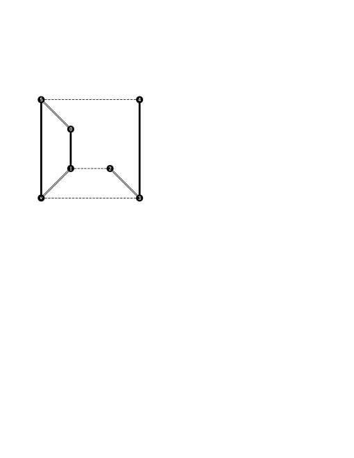
In other words, is the subset of that contains all pairs of edges where both and are in and edges obtain the same local color whenever they are in the same equivalence class of . As an example consider the PSP in Figure 1(d). The relation has three equivalence classes (highlighted by thick, dashed and double-lined edges). Note, just contains one equivalence class. Hence, .
For a given subset we set
The transitive closure of is then called the global coloring with respect to . As shown in [8], we have the following theorem.
Theorem 3.
Let be a given graph and . Then
For later reference and for the design of the recognition algorithm we list the following three lemmas about relevant properties of the PSP.
Lemma 4 ([8]).
Let G=(V,E) be a given graph and be a PSP of an arbitrary vertex . If are primal edges that are not in relation , then and span a unique chordless square with a unique top vertex in .
Conversely, suppose that is a non-primal vertex of . Then there is a unique chordless square in that contains , and that is spanned by edges with .
Lemma 5 ([8]).
Let G=(V,E) be a given graph and be a non-primal edge of a PSP of an arbitrary vertex . Then is opposite to exactly one primal edge in , and .
Lemma 6 ([8]).
Let G=(V,E) be a given graph and such that is connected. Then each vertex meets every equivalence class of in .
3 Quasi Cartesian Products
Given a Cartesian product of two connected, prime graphs and , one can recover the factors and as follows: the product relation has two equivalence classes, say and , and the connected components of the graph are all isomorphic copies of the factor , or of the factor , see Figure 1(a). This property naturally extends to products of more than two prime factors.
We already observed that is finer than any equivalence relation that satisfies the square property. Hence the equivalence classes of are unions of -classes. This also holds for . It is important to keep in mind that can be trivial, that is, it consists of a single equivalence class even when has more than one equivalence class.
We call all graphs with a non-trivial equivalence relation that is defined on and satisfies the square property quasi (Cartesian) products. Since for every such relation , it follows that must have at least two equivalence classes for any quasi product. By Theorem 3 we have . In other words, quasi products can be defined as graphs where the PSP’s of all vertices are non-trivial, that is, none of the PSP’s is a star , and in addition, where the union over all yields a non-trivial .
Consider the equivalence classes of the relation of the graph of Figure 1(b). It has two equivalence classes, and locally looks like a Cartesian product, but is actually reminiscent of a Möbius band. Notice that the graph in Figure 1(b) is prime with respect to Cartesian multiplication, although has two equivalence classes: all components of the first class are paths of length , and there are two components of the other -class, which do not have the same size. Locally this graph looks either like or .


In fact, the graph in Figure 1(b) is a so-called Cartesian graph bundle [11], where Cartesian graph bundles are defined as follows: Let and be graphs. A graph is a (Cartesian) graph bundle with fiber over the base if there exists a weak homomorphism222A weak homomorphism maps edges into edges or single vertices. such that
-
(i)
for any , the subgraph (induced by) is isomorphic to , and
-
(ii)
for any , the subgraph is isomorphic to
The graph of Figure 1(c) shows that not all quasi Cartesian products are graph bundles. On the other hand, not every graph bundle has to be a quasi product. The standard example is the complete bipartite graph . It is a graph bundle with base and fiber , but has only one -class.
Note, in [8] we considered ”approximate products” which were first introduced in [7, 6]. As approximate products are all graphs that have a (small) edit distance to a non-trivial product graph, it is clear that every bundle and quasi product can be considered as an approximate product, while the converse is not true. For example, consider the graph in Figure 1(d). Here, has only one equivalence class. However, the relation has, in this case, three equivalence classes (highlighted by thick, dashed and double-lined edges).
Because of the local product-like structure of quasi Cartesian products we are led to the following conjecture:
Conjecture 7.
Quasi Cartesian products can be reconstructed in essentially the same time from vertex-deleted subgraphs as Cartesian products.
4 Recognition Algorithms
4.1 Computing the Local and Global Coloring
For a given graph , let be an arbitrary subset of the vertex set of such that the induced subgraph is connected. Our approach for the computation is based on the recognition of all PSP’s with , and subsequent merging of their local colorings. The subroutine computing local colorings calls the vertices in BFS-order with respect to an arbitrarily chosen root .
Let now us briefly introduce several additional notions used in the PSP recognition algorithm. At the start of every iteration we assign pairwise different temporary local colors to the primal edges of every PSP. These colors are then merged in subroutine processes to compute local colors associated with every PSP. Analogously, we use temporary global colors that are initially assigned to every edge incident with the root .
For any vertex of distance two from a PSP center we store attributes called first and second primal neighbor, that is, references to adjacent primal vertices from which was ”visited” (in pseudo-code attributes are accessed by and ). When is found to have at least two primal neighbors we add to , which is a stack of candidates for non-primal vertices of . Finally, we use incidence and absence lists to store recognized squares spanned by primal edges. Whenever we recognize that two primal edges span a square we put them into the incidence list. If we find out that a pair of primal edges cannot span a unique chordless square with unique top vertex, then we put it into the absence list. Note that the above structures are local and are always associated with a certain PSP recognition subroutine (Algorithm 4.1). Finally, we will ”map” local colors to temporary global colors via temporary vectors which helps us to merge local with global colors.
Algorithm 4.1 computes a local coloring for given PSP’s and merges it with the global coloring where is the set of treated centers. Algorithm 4.1 summarizes the main control structure of the local approach.
[PSP recognition] Input: Connected graph , PSP center , global coloring , where is the set of treated centers and where the subgraph induced by is connected. Output: New temporary global coloring .
-
1.
Initialization.
-
2.
FOR every neighbor of DO:
-
(a)
FOR every neighbor of (except ) DO:
-
i.
IF is primal w.r.t. THEN put pair of primal edges to absence list.
-
ii.
ELSEIF was not visited THEN set .
-
iii.
ELSE ( is not primal and was already visited) DO:
-
A.
IF only one primal neighbor of was recognized so far, then DO:
-
•
Set .
-
•
IF is not in incidence list, then add to the stack and add the pair to incidence list.
-
•
ELSE ( and span more squares) add pair to absence list.
-
•
-
B.
ELSE:
-
•
Add all pairs formed by primal edges to absence list, where are first and second primal neighbors of .
-
•
-
A.
-
i.
-
(a)
-
3.
Assign pairwise different temporary local colors to primal edges.
-
4.
FOR any pair of primal edges and DO:
-
(a)
IF is contained in absence list THEN merge temporary local colors of and .
-
(b)
IF is not contained in incidence list THEN merge temporary local colors of and .
(Resulting merged temporary local colors determine local colors of primal edges in . We will reference them in the following steps.).
-
(a)
-
5.
FOR any primal edge DO:
-
(a)
IF was already assigned some temporary global color THEN
-
i.
IF local color of was already mapped to some temporary global color , where , THEN merge and .
-
ii.
ELSE map local color to .
-
i.
-
(a)
-
6.
FOR any vertex from stack DO:
-
(a)
Check local colors of primal edges and (where are first and second primal neighbor of , respectively).
-
(b)
IF they differ in local colors THEN
-
i.
IF there was defined temporary global color for THEN
-
A.
IF local color of was already mapped to some temporary global color , where THEN merge and .
-
B.
ELSE map local color to .
-
A.
-
ii.
IF there was already defined temporary global color for THEN:
-
A.
IF local color of was already mapped to some temporary global color , where THEN merge and .
-
B.
ELSE map local color to .
-
A.
-
i.
-
(a)
-
7.
Take every edge of the PSP that was not colored by any temporary global color up to now and assign it , where is the temporary global color to which the local color of or the local color of its opposite primal edge was mapped.
(If there is a local color that was not mapped to any temporary global color, then we create a new temporary global color and assign it to all edges of color ).
{algo}
[Computation of ] Input: A connected graph , s.t. the induced subgraph is connected and, an arbitrary vertex . Output: Relation .
-
1.
Initialization.
-
2.
Set sequence of vertices that form in BFS-order with respect to .
-
3.
Set .
-
4.
Assign pairwise different temporary global colors to edges incident to .
-
5.
FOR any vertex from sequence DO:
-
(a)
Use Algorithm 4.1 to compute .
-
(b)
Add to .
-
(a)
In order to show that Algorithm 4.1 correctly recognizes the local coloring, we define the (temporary) relations and for a chosen vertex : Two primal edges of are
-
•
in relation if they are contained in the incidence list and
-
•
in relation if they are contained in the absence list
after Algorithm 4.1 is executed for . Note, we denote by the complement of , which contains all pairs of primal edges of PSP that are not listed in the incidence list.
Lemma 8.
Let and be two primal edges of the PSP . If and span a square with some non-primal vertex as unique top-vertex, then .
Proof 4.1.
Let and be primal edges in that span a square with unique top-vertex , where is non-primal. Note, since is the unique top vertex, the vertices and are its only primal neighbors. W.l.o.g. assume that for vertex no first primal neighbor was assigned and let first and then be visited. In Step 2a vertex is recognized and the first primal neighbor is determined in Step 2(a)ii. Take the next vertex . Since is not primal and was already visited, we are in Step 2(a)iii. Since only one primal neighbor of was recognized so far, we go to Step 2iiiA. If is not already contained in the incidence list, it will be added now and thus, .
Corollary 9.
Let and be two adjacent distinct primal edges of the PSP . If , then and do not span a square or span a square with non-unique or primal top vertex. In particular, contains all pairs that do not span any square.
Proof 4.2.
The first statement is just the contrapositive of the statement in Lemma 8. For the second statement observe that if and are two distinct primal edges of that do not span a square, then the vertices and do not have a common non-primal neighbor . It is now easy to verify that in none of the substeps of Step 2 the pair is added to the incidence list, and thus, .
Lemma 10.
Let and be two primal edges of the PSP that are in relation . Then and do not span a unique chordless square with unique top vertex.
Proof 4.3.
Let and be primal edges of . Then pair is inserted to absence list in:
-
a)
Step 2(a)i, when and are adjacent. Then no square spanned by and can be chordless.
-
b)
Step 2iiiA (ELSE-condition), when is already listed in the incidence list and another square spanned by and is recognized. Thus, and do not span a unique square.
-
c)
Step 2iiiB, when and span a square with top vertex that has more than two primal neighbors and at least one of the primal vertices and are recognized as first or second primal neighbor of . Thus and span a square with non-unique top vertex.
Lemma 11.
Relation contains all pairs of primal edges of that satisfy at least one of the following conditions:
-
a)
and span a square with a chord.
-
b)
and span a square with non-unique top vertex.
-
c)
and span more than one square.
Proof 4.4.
Let and be primal edges of w[PSP] .
-
a)
If and span a square with a chord, then and are adjacent or the top vertex of the spanned square is primal and thus, there is a primal edge . In the first case, we can conclude analogously as in the proof of Lemma 10 that . In the second case, we analogously obtain and therefore, .
-
b)
Let and span a square with non-unique top vertex . If at least one of the primal vertices is a first or second neighbor of then and are listed in the absence list, as shown in the proof of Lemma 10. If and are neither first nor second primal neighbors of , then both edges and will be added to the absence list in Step 2iiiB, together with the primal edge , where is the first recognized primal neighbor of . In other words, and hence, .
-
c)
Let and span two squares with top vertices and , respectively and assume w.l.o.g. that first vertex is visited and then . If both vertices and are recognized as first and second primal neighbors of and , then is added to the incidence list when visiting in Step 2iiiA. However, when we visit , then we insert to the absence list in Step 2iiiA, because this pair is already included in the incidence list. Thus, . If at least one of the vertices does not have and as first or second primal neighbor, then and must span a square with non-unique top vertex. Item b) implies that .
Lemma 12.
Let be a non-primal edge and be two distinct primal edges of . Let . Then .
Proof 4.5.
Since the edge is non-primal, is not incident with the center . Recall, by the definition of , two distinct edges can be in relation only if they have a common vertex or are opposite edges in a square. To prove our lemma we need to investigate the three following cases, which are also illustrated in Figure 2:
-
a)
Suppose both edges and are incident with . Then and span a triangle and consequently will be added to the absence list in Step 2(a)i.
- b)
-
c)
Suppose only has a common vertex with and is opposite to in a square. Again we need to consider two cases (see Figure 2 c)). Since and are adjacent and , we can conclude that either no square is spanned by and , or that the square spanned by and is not chordless or not unique. Its easy to see that in the first case the edges and are contained in a common triangle and thus will be added to the absence list in Step 2(a)i. In the second case span a square which has a chord or has a non-unique top vertex. In both cases Lemma 11 implies that and are in relation .

Lemma 13.
Let and be distinct primal edges of the PSP . Then if and only if .
Proof 4.6.
Assume first that . By Corollary 9, if , then and do not span a common square, or span a square with non-unique or primal top vertex. In the first case, and are in relation and consequently also in relation . On the other hand, if and span square with non-unique top vertex then, by Lemma 4, and are in relation as well. Finally, if and span a square with primal top vertex , then this square has a chord and . If , then Lemma 10 implies that and do not span unique chordless square with unique top vertex. Again, by Lemma 4, we infer that . Hence, , and consequently, .
Now, let . Then there is a sequence , , with for . By definition of , two primal edges are in relation if and only if they do not span a unique and chordless square. Corollary 9 and Lemma 11 imply that all these pairs are contained in . Hence, any two consecutive primal edges and contained in the sequence are in relation . Assume that there is an edge that is not incident to the center and thus, non-primal. By the definition of , and since , we can conclude that the edges and must be primal in . Lemma 12 implies that and must be in relation . By removing all edges from that are not incident with we obtain a sequence of primal edges. By analogous arguments as before, all pairs of must be contained in . By transitivity, and are also in .
Corollary 14.
Let and be primal edges of the PSP . Then if and only if and have the same local color in .
Proof 4.7.
Lemma 15.
Let be a global coloring associated with a set of treated centers and assume that the induced subgraph is connected. Let be a vertex that is not contained in but adjacent to a vertex in . Then Algorithm 4.1 computes the global coloring by taking and as input.
Proof 4.8.
Let be a set of PSP centers and let be a given center of PSP where and is connected. In Step 2 of Algorithm 4.1 we compute the absence and incidence lists. In Step 3, we assign pairwise different temporary local colors to any primal edge adjacent to . Two temporary local colors and are then merged in Step 4 if and only if there exists some pair of primal edges where is colored with and with . Therefore, merged temporary local colors reflect equivalence classes of containing the primal edges incident to . By Corollary 14, classes indeed determine the local colors of primal edges in .
Note, if one knows the colors of primal edges incident to , then it is very easy to determine the set of non-primal edges of , as any two primal edges of different equivalence classes span a unique and chordless square. In Step 6, we investigate each vertex from stack and check the local colors of primal edges and , where and are the first and second recognized primal neighbors of , respectively. If and differ in their local colors, then and are non-primal edges of , as follows from the PSP construction. Recall that the stack contains all vertices that are at distance two from center and which are adjacent to at least two primal vertices. In other words, the stack contains all non-primal top vertices of all squares spanned by primal edges. Consequently, we claim that all non-primal edges of the PSP are treated in Step 6. Note that non-primal edges have the same local color as their opposite primal edge, which is unique by Lemma 5.
As we already argued, after Step 4 is performed we know, or can at least easily determine all edges of and their local colors. Recall that local colors define the local coloring . Suppose, temporary global colors that correspond to the global coloring are assigned. Our goal is to modify and identify temporary global colors such that they will correspond to the global coloring . Let be the classes of (local classes) and be the classes of (global classes). When a local class and a global class have a nonempty intersection, then we can infer that all their edges must be contained in a common class of . Note, by means of Lemma 6, we can conclude that for each local class there is a global class such that , see also [8]. In that case we need to guarantee that edges of and will be colored by the same temporary global color. Note, in the beginning of the iteration two edges have the same temporary global color if and only if they lie in a common global class.
In Step 5 and Step 6, we investigate all primal and non-primal edges of . When we treat first edge that is colored by some local color , that is , and has already been assigned some temporary global color , and therefore , then we map to . Thus, we keep the information that . In Step 7, we then assign temporary global color to any edge of that is colored by the local color . If the local color is already mapped to some temporary global color , and if we find another edge of that is colored by and simultaneously has been assigned some different temporary global color , then we merge and in Step 5(a)i. Obviously this is correct, since and , and hence and must be contained in a common equivalence class of . Recall, for each local class there is a global class such that . This means that every local color is mapped to some global color, and consequently there is no need to create a new temporary global color in Step 7.
Therefore, whenever local and global classes share an edge, then all their edges will have the same temporary global color at the end of Step 7. On the other hand, when edges of two different global classes are colored by the same temporary global color, then both global classes must be contained in a common class of .
Hence, after the performance of Step 7, the merged temporary global colors determine the equivalence classes of .
Lemma 16.
Let be a connected graph, s.t. is connected, and an arbitrary vertex of . Then Algorithm 4.1 computes the global coloring by taking , and as input.
Proof 4.9.
In Step 2 we define the BFS-order in which the vertices will be processed and store this sequence in . In Step 4 we assign pairwise different temporary global colors to all edges that are incident with . In Step 5 we iterate over all vertices of the given induced connected subgraph of . For every vertex we execute Algorithm 4.1. Lemma 15 implies that in the first iteration, we correctly compute the local colors for , and consequently also . Obviously, whenever we merge two temporary local colors of two primal edges in the first iteration, then we also merge their temporary global colors. Consequently, the resulting temporary global colors correspond to the global coloring after the first iteration. Lemma 15 implies that after all iterations are performed, that is, all vertices in are processed, the resulting temporary global colors correspond to for the given input set .
For the global coloring, Theorem 3 implies that . This leads to the following corollary.
Corollary 17.
Let be a connected graph and an arbitrary vertex of . Then Algorithm 4.1 computes the global coloring by taking , and as input.
4.2 Time Complexity
We begin with the complexity of merging colors. We have global and local colors, and will define local and global color graphs. Both graphs are acyclic temporary structures. Their vertex sets are the sets of temporary colors in the initial state. In this state the color graphs have no edges. Every component is a single vertex and corresponds to an initial temporary color. Recall that we color edges of graphs, for example the edges of or . The color of an edge is indicated by a pointer to a vertex of the color graph. These pointers are not changed, but the colors will correspond to the components of the color graph. When two colors are merged, then this reflected by adding an edge between their respective components.
The color graph is represented by an adjacency list as described in [5, Chapter 17.2] or [9, pp. 34 -37]. Thus, working with the color graph needs space when colors are used. Furthermore, for every vertex of the color graph we keep an index of the connected component in which the vertex is contained. We also store the actual size of every component, that is, the number of vertices of this component.
Suppose we wish to merge temporary colors of edges and that are identified with vertices , respectively , in the color graph. We first check whether and are contained in the same connected component by comparing component indices. If the component indices are the same, then and already have the same color, and no action is necessary. Otherwise we insert an edge between and in the color graph. As this merges the components of and we have to update component indices and the size. The size is updated in constant time. For the component index we use the index of the larger component. Thus, no index change is necessary for the larger component, but we have to assign the new index to all vertices of the smaller component.
Notice that the color graph remains acyclic, as we only add edges between different components.
Lemma 18.
Let be a graph with and . The components of consist of single vertices. We assign component index to every component . For let denote the graph that results from by adding an edge between two distinct connected components, say and . If , we use the the component index of for the new component and assign it to every vertex of .
Then every is acyclic, and the total cost of merging colors is .
Proof 4.10.
Acyclicity is true by construction.
A vertex is assigned a new component index when its component is merged with a larger one. Thus, the size of the component at least doubles at every such step. Because the maximum size of a component is bounded by , there can be at most reassignments of the component index for every vertex. As there are vertices, this means that the total cost of merging colors is .
The color graph is used to identify temporary local, resp., global colors. Based on this, we now define the local and global color graph.
Assigned labels of the vertices of the global color graph are stored in the edge list, where any edge is identified with at most one such label. A graph is represented by an extended adjacency list, where for any vertex and its neighbor a reference to the edge (in the edge list) that connects them is stored. This reference allows to access a global temporary color from adjacency list in constant time.
In every iteration of Algorithm 4.1, we recognize the PSP for one vertex by calling Algorithm 4.1. In the following paragraph we introduce several temporary attributes and matrices that are used in the algorithm.
Suppose we execute an iteration that recognizes some PSP . To indicate whether a vertex was treated in this iteration we introduce the attribute , that is, when vertex is visited in this iteration we set . Any value different from means that vertex was not yet treated in this iteration. Analogously, we introduce the attribute to indicate that a vertex is adjacent to the current center . The attribute maps primal vertices to the indices of rows and columns of the matrices and . For any vertex that is at distance two from the center we store its first and second primal neighbor and in the attributes and . Furthermore, we need to keep the position of and in the edge list to get their temporary global colors. For this purpose, we use attributes and . Attribute helps us to map temporary local colors to the vertices of the global color graph. Any vertex that is at distance two from the center and has a least two primal neighbors is a candidate for a non-primal vertex. We insert them to the . The temporary structures help to access the required information in constant time:
-
•
vertex has been already visited in the current iteration. -
•
vertex is adjacent to center . -
•
pair of primal edges is missing in the incidence list. -
•
pair of primal edges was inserted to the absence list. -
•
is the first recognized primal neighbor of the non-primal vertex . -
•
edge joins the non-primal vertex with its first recognized primal neighbor (it is used to get the temporary global color from the edge list). -
•
local color is mapped to temporary global color (i.e. there exists an edge that is colored by both colors).
Note that the temporary matrices and have dimension and that all their entries are set to zero in the beginning of every iteration.
Theorem 19.
For a given connected graph with maximum degree and , Algorithm 4.1 runs in time and space.
Proof 4.11.
Let be a given graph with edges and vertices. In Step 1 of Algorithm 4.1 we initialize all temporary attributes and matrices. This consumes time and space, since is connected, and hence, . Moreover, we set all temporary colors of edges in the edge list to zero, which does not increase the time and space complexity of the initial step. Recall that we use an extended adjacency list, where every vertex and its neighbors keep the reference to the edge in the edge list that connects them. To create an extended adjacency list we iterate over all edges in the edge list, and for every edge we set a new entry for the neighbor for and, simultaneously, we add a reference . The same is done for vertex . It can be done in time and space.
In Step 2 of Algorithm 4.1, we build a sequence of vertices in BFS-order starting with , which is done in time in general. Since is connected, the BFS-ordering can be computed in time. Step 3 takes constant time. In Step 4 we initialize the global color graph that has vertices (bounded by in general). As we already showed, all operations on the global color graph take time and space. We proceed to traverse all neighbors of the root (via the adjacency list) and assign them unique labels in edge list, that is, every edge gets the label . In this way, we initialize pairwise different temporary global colors of edges incident with , that is, to vertices of the global color graph. Using the extended adjacency list, we set the label to an edge in the edge list in constant time. In Step 5 we run Algorithm 4.1 for any vertex from the defined BFS-sequence.
In the remainder of this proof, we will focus on the complexity of Algorithm 4.1. Suppose we perform Algorithm 4.1 for vertex to recognize the PSP . The recognition process is based on temporary structures. We do not need to reset any of these structures, for any execution of Algorithm 4.1 for a new center , except and . This is done in Step 1. Further, we set here the attribute for every primal vertex , such that every vertex has assigned a unique number from . Finally, we traverse all neighbors of the center and for each of them we set to . Hence, the initial step of Algorithm 4.1 is done in time.
Step 2a is performed for every neighbor of every primal vertex. The number of all such neighbors is at most . For every treated vertex, we set attribute to . This allows us to verify in constant time that a vertex was already visited in the recognition subroutine Algorithm 4.1.
If the condition in Step 2(a)i is satisfied, then we put primal edges and to the absence list. By the previous arguments, this can be done in constant time by usage of and .
If the condition in Step 2(a)ii is satisfied, we set vertex as first primal neighbor of vertex . For this purpose, we use the attribute . We also set , where is a reference to the edge in the edge list that connects and . This reference is obtained from the extended adjacency list in constant time. Recall, the edge list is used to store the labels of vertices of the global color graph for the edges of a given graph, that is, the assignment of temporary global colors to the edges. Using , we are able to directly access the temporary global color of edge in constant time.
Step 2(a)iii is performed when we try to visit a vertex from some vertex where has been already visited before from some vertex . If is the only recognized primal neighbor of , then we we perform analogous operations as in the previous step. Moreover. if is not contained in the incidence list, then we set as second primal neighbor of , add to the incidence list and add to the stack. Otherwise we add to the absence list. The number of operations in this step is constant.
If has more recognized primal neighbors we process case B. Here we just add all pairs formed by to absence list. Again, the number of operations is constant by usage of and matrices and .
In Step 3[,] we assign pairwise different temporary local colors to the primal edges. Assume the neighbors of the center are labeled by , then we set value to . In Step 4a we iterate over all entries of the . For all pairs of edges that are in the absence list we check whether they still have different temporary local colors and if so, we merge their temporary local colors by adding a respective edge in the local color graph. Analogously we treat all pairs of edges contained in the in Step 4b. Here we merge temporary local colors of primal edges and when the pair is missing. To treat all entries of the and we need to perform iterations. Recall, the temporary local color of the primal edge is equal to the index of the connected component in the local color graph, in which vertex is contained. Thus, the temporary local color of this primal edge can be accessed in constant time. As we already showed, the number of all operations on the local color graph is bounded by . Hence, the overall time complexity of both Steps 3 and 4 is .
In Step 5 we map temporary local colors of primal edges to temporary global colors. For this purpose, we use the attribute . The temporary global color of every edge can be accessed by the extended adjacency list, the edge list and the global color graph in constant time. Since we need to iterate over all primal vertices, we can conclude that Step 5 takes time.
In Step 6 we perform analogous operations for any vertex from Stack as in Step 5. In the worst case, we add all vertices that are at distance two from the center to the stack. Hence, the size of the stack is bounded by . Recall that the first and second primal neighbor and of every vertex from the stack can be directly accessed by the attributes and . On the other hand, the temporary global colors of non-primal edges and can be accessed directly by the attributes and . Thus, all needful information can be accessed in constant time. Consequently, the time complexity of this step is bounded by .
In the last step, Step 7, we iterate over all edges of the recognized PSP. Note, the list of all primal edges can be obtained from the extended adjacency list. To get all non-primal edges we iterate over all vertices from the stack and use the attributes and , which takes time. The remaining operations can be done in constant time.
To summarize, Algorithm 4.1 runs in time. Consequently, Step 5 of Algorithm 4.1 runs in time, which defines also the total time complexity of Algorithm 4.1. The most space consuming structures are the edge list and the extended adjacency list ( space) and the temporary matrices and space). Hence, the overall space complexity is .
Since quasi Cartesian products are defined as graphs with non-trivial , Theorem 19 and Corollary 17 imply the following corollary.
Corollary 20.
For a given connected graph with bounded maximum degree Algorithm 4.1 (with slight modifications) determines whether is a quasi Cartesian product in time and space.
4.3 Parallel Processing
The local approach allows the parallel computation of on multiple processors. Consider a graph with vertex set . Suppose we are given a decomposition of into parts such, that , where the subgraphs induced by are connected, and the number of edges whose endpoints lie in different partitions is small (we call such decomposition good). Then algorithm 4.1 can be used to compute the colorings , where every instance of the algorithm can run in parallel. The resulting global colorings are used to compute . Let us sketch the parallelization.
{algo}
[Parallel recognition of ] Input: A graph , and a good decomposition . Output: Relation .
-
1.
For every partition concurrently compute global coloring ():
-
(a)
Take all vertices of and order them in BFS to get sequence .
-
(b)
Set .
-
(c)
Assign pairwise different temporary global colors to edges incident to first vertex in .
-
(d)
For any vertex from sequence do:
-
i.
Use Algorithm 4.1 to compute .
-
ii.
Put all edges that were treated in previous step and have at least one endpoint not in partition to stack .
-
iii.
Add to .
-
i.
-
(a)
-
2.
Run concurrently for every partition to merge all global colorings ():
-
(a)
For each edge from stack , take all its assigned global colors and merge them.
-
(a)
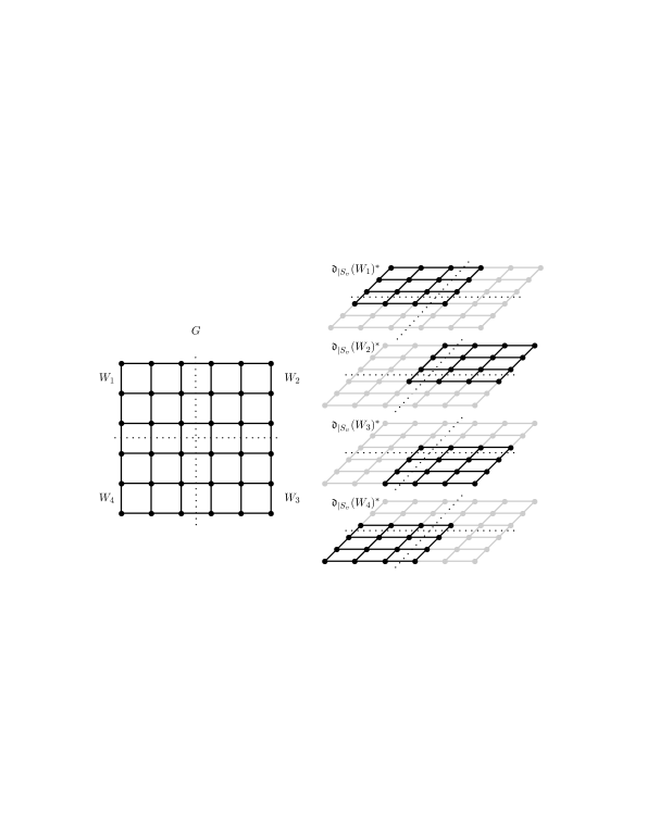
Figure 3 shows an example of decomposed vertex set of a given graph . The computation of global colorings associated with the individual sets of the partition can be done then in parallel. The edges that are colored by global color when the partition is treated are highlighted by bold black color. Thus we can observe that many edges will be colored by more then one color.
Notice that we do not treat the task of finding a good partition. With the methods of [4] this is possible with high probability in time, where is the number of vertices.
References
- [1] W. Dörfler. Some results on the reconstruction of graphs. In Infinite and finite sets (Colloq., Keszthely, 1973; dedicated to P. Erdős on his 60th birthday), Vol. I, pages 361–363. Colloq. Math. Soc. János Bolyai, Vol. 10. North-Holland, Amsterdam, 1975.
- [2] J. Feigenbaum. Product graphs: some algorithmic and combinatorial results. Technical Report STAN-CS-86-1121, Stanford University, Computer Science, 1986. PhD Thesis.
- [3] Johann Hagauer and Janez Žerovnik. An algorithm for the weak reconstruction of Cartesian-product graphs. J. Combin. Inform. System Sci., 24(2-4):87–103, 1999.
- [4] Shay Halperin and Uri Zwick. Optimal randomized EREW PRAM algorithms for finding spanning forests. J. Algorithms, 39(1):1–46, 2001.
- [5] R. Hammack, W. Imrich, and S. Klavžar. Handbook of Product Graphs. Discrete Mathematics and its Applications. CRC Press, 2nd edition, 2011.
- [6] M. Hellmuth. A local prime factor decomposition algorithm. Discrete Mathematics, 311(12):944–965, 2011.
- [7] M. Hellmuth, W. Imrich, W. Klöckl, and P. F. Stadler. Approximate graph products. European J. Combin., 30:1119 – 1133, 2009.
- [8] M. Hellmuth, W. Imrich, and T. Kupka. Partial star products: A local covering approach for the recognition of approximate Cartesian product graphs. Math. Comput. Sci, 2013.
- [9] W. Imrich and S Klavžar. Product graphs. Wiley-Interscience Series in Discrete Mathematics and Optimization. Wiley-Interscience, New York, 2000.
- [10] W. Imrich and I. Peterin. Recognizing Cartesian products in linear time. Discrete Mathematics, 307(3 – 5):472 – 483, 2007.
- [11] W. Imrich, T. Pisanski, and J. Žerovnik. Recognizing Cartesian graph bundles. Discr. Math, 167-168:393–403, 1997.
- [12] W. Imrich and J. Žerovnik. Factoring Cartesian-product graphs. J. Graph Theory, 18(6):557–567, 1994.
- [13] T. Kupka. A local approach for embedding graphs into Cartesian products. PhD thesis, VSB-Technical University of Ostrava, 2013.
- [14] T. Pisanski, B. Zmazek, and J. Žerovnik. An algorithm for -convex closure and an application. Int. J. Comput. Math., 78(1):1–11, 2001.
- [15] G. Sabidussi. Graph multiplication. Math. Z., 72:446–457, 1960.