The influence of defects on the conductivity of graphene within the effective theory approach

Abstract

The results of the simulations by Monte Carlo method of graphene with structural defects are presented. The calculations are performed within an effective quantum field theory with non-compact $3\hm+1$–dimensional Abelian gauge field and $2\hm+1$–dimensional Kogut-Susskind fermions. It was found that defects shift the phase transition point semimetal-insulator towards higher values of a substrate permittivity.

05.10.Ln, 71.30.+h, 72.80.Vp

1 INTRODUCTION

At present there exists a considerable interest to the unique electronic properties of graphene [1, 2, 3]. It has been shown that many-body effects play an important role in the description of physical phenomena in graphene.

Quasiparticles in graphene interact via Coulomb law with the effective coupling constant $\alpha_{eff}\sim\alpha_{em}/v_{f}\sim 300/137\sim$ 2. Thus the system is strongly coupled and the application of analytical methods to study the properties of graphene is difficult and numerical simulation is an adequate method for the investigations.

Below we present the results of the study of the insulator-semimetal phase transition which is rather important for practical applications of graphene. The influence of the dielectric properties of the substrate, external fields, structural defects to the conductivity of a graphene may shift the position of the phase transition. Below we present the study of the conductivity of the monolayer graphene as a function of a concentration of defects in the effective field model.

Usually graphene is placed on the substrate and the effective coupling is $\alpha_{eff}=2\alpha_{em}/(v_{f}(\epsilon+1))$, where $\epsilon$ is the dielectric permittivity of graphene. The use of substrates with different values of dielectric permittivity $\epsilon$ alters the interaction between quasiparticles.

It has been shown in [7, 8, 9] that a decrease of the substrate permittivity leads to the shift of the transition of graphene from semi-metal phase to the insulator phase. The phase transition occurs for the values of permittivity $\epsilon_{c}\sim$ 4. Recent experimental results show [4] that graphene is in semi-metal phase even in vacuum ($\epsilon_{c}=$ 1). The possible explanation of this discrepancy is a modification (screening) of the Coulomb potential at short distances [5]. However the phase transition still exists for $\epsilon_{c}<$ 1 even in the case of screened Coulomb potential. Also qualitative behaviour of chiral condensate, which is the order parameter of the phase transition is quite similar to the effective field theory with unscreened Coulomb potential. So we can hope that influence of defects in effective field theory will describe real physics properly at qualitative level.

2 DETAILS OF THE CALCULATIONS

The Euclidean partition function for the electrons in graphene is calculated using the Monte Carlo method [1, 2, 3, 6]

$$\mathcal{Z}=\int\mathcal{D}\bar{\psi}\mathcal{D}\psi\mathcal{D}A_{0}\exp\left(-\frac{1}{2}\int d^{4}x\left(\partial_{i}A_{0}\right)^{2}-\right.$$

$$\left.-\int d^{3}x\,\bar{\psi}_{f}\,\left(\Gamma_{0}\,\left(\partial_{0}-igA_{0}\right)-\sum\limits_{i=1,2}\Gamma_{i}\partial_{i}\right)\psi_{f}\right),$$ (1)

where $A_{0}$ is the zero component of the vector potential of the electromagnetic field, $\Gamma_{\mu}$ are the Euclidean gamma - matrices and $\psi_{f}$, ($f\hm=1,2$) are two flavors of Dirac fermions, corresponding to the two spin components of the electronic excitations in graphene, the effective coupling constant $g^{2}\hm=2\alpha_{em}/(v_{F}(\epsilon+1))$ ($\hbar\hm=\hm c\hm=1$). The zero component of the vector potential $A_{0}$ satisfies the periodic boundary conditions in space and time $A_{0}(t=0)=A(t=1/T)$, where $T$ is the temperature. In the absence of the magnetic field fermionic fields obey periodic boundary conditions in space and antiperiodic boundary conditions in time $\psi_{f}(t=0)=-\psi_{f}(t=1/T)$. The partition function (2) does not include the vector part of the potential, $A_{i}$, since it is suppressed by the Fermi velocity $v_{f}\sim 1/300$.

For a discretization of the fermionic part of the action in (2) we use the Kogut-Susskind fermions [10, 11]. One kind of these fermions in $2\hm+1$ dimensions corresponds to the two flavors of ordinary Dirac fermions [10, 11, 12], making them particularly suitable for the simulation of the quantum field theory of graphene. The action for Kogut-Susskind fermions, interacting with an abelian lattice gauge field has the form

$$S_{\Psi}\left[\bar{\Psi}_{x},\Psi_{x},\theta_{x,\,\mu}\right]=\sum\limits_{x,y}\bar{\Psi}_{x}\,D_{x,y}\left[\theta_{x,\,\mu}\right]\,\Psi_{y}=$$

$$=\frac{1}{2}\,\sum\limits_{x}\,\delta_{x_{3},\,0}\,\left(\sum\limits_{\mu=0,1,2}\bar{\Psi}_{x}\alpha_{x,\mu}e^{i\theta_{x,\,\mu}}\Psi_{x+\hat{\mu}}-\right.$$

$$\left.-\sum_{\mu=0,1,2}\bar{\Psi}_{x}\alpha_{x,\mu}e^{-i\theta_{x,\,\mu}}\Psi_{x-\hat{\mu}}+m{\bar{\Psi}}_{x}\Psi_{x}\right),$$ (2)

where lattice coordinates are: $x^{\mu}\hm=0\ldots L_{\mu}\hm-1$, and $x^{3}$ is bounded by the condition $x^{3}\hm=0$ (the graphene sheet lie in the plane $x^{3}=0$), $\bar{\Psi}_{x}$ is one-component Grassmann field, $\alpha_{x,\mu}\hm=(-1)^{x_{0}+\ldots+x_{\mu-1}}$, and $\theta_{x,\,\mu}$ are the variables on the links, lattice analogues of the vector potential $A_{\mu}\left(x\right)$ (only $\theta_{x,\,0}$ is nonzero due to the suppression of magnetic field), $D_{x,y}$ is the Dirac operator for the Kogut-Susskind fermions. $m$ is an artificial mass. It should be introduced in order to make the lattice Dirac operator invertible. We perform calculations for several different values of $m$ and obtain real physical values of all quantities in the limit $m\rightarrow 0$.

For the discretization of the electromagnetic field in the action (2) we use the non-compact action for the gauge fields:

$$S_{g}\left[\theta_{x,\,\mu}\right]=\frac{\beta}{2}\,\sum\limits_{x}\sum\limits^{3}_{i=1}\left(\theta_{x,\,0}-\theta_{x+\hat{i},\,0}\right)^{2},$$ (3)

where the sum over $x$ is performed over the entire 4D lattice. The constant $\beta$ is defined as follows

$$\beta\equiv\frac{1}{g^{2}}=\frac{v_{F}}{4\pi e^{2}}\,\frac{\epsilon+1}{2},$$ (4)

where the factor $\frac{\epsilon+1}{2}$ is due to the screening of the electrostatic interactions.

Since the fermion action (2) is bilinear in the fermion fields, it can be integrated out, which gives

$$\mathcal{Z}=\int\mathcal{D}\bar{\Psi}_{x}\,\mathcal{D}\Psi_{x}\,\mathcal{D}\theta_{x,\,0}\,$$

$$\exp\left(-S_{g}\left[\theta_{x,\,0}\right]-S_{\Psi}\left[\bar{\Psi}_{x},\Psi_{x},\theta_{x,\,0}\right]\right)=$$

$$=\int\mathcal{D}\theta_{x,\,0}\,\det\left(D\left[\theta_{x,\,0}\right]\right)\exp{\left(-S_{g}\left[\theta_{x,\,0}\right]\right)}.$$ (5)

Thus, we get the effective action

$$S_{eff}\left[\theta_{x,\,0}\right]=S_{g}\left[\theta_{x,\,0}\right]-\ln\det\left(D\left[\theta_{x,\,0}\right]\right),$$ (6)

which includes the determinant $\det\left(D\left[\theta_{x,\,\mu}\right]\right)$ of the Dirac operator $D_{x,y}\left[\theta_{x,\,\mu}\right]$ (2).

For the numerical simulations the standard hybrid Monte-Carlo method was used, allowing to generate gauge field configurations $\theta_{x,\,0}$ with statistical weight $\exp{\left(-S_{eff}\left[\theta_{x,\,0}\right]\right)}$ [10, 11].

To find the semimetal-insulator phase transition it is convenient to use the order parameter the chiral fermion condensate $\langle\,\bar{\psi}\,\psi\,\rangle$. In the semi-metal phase the chiral condensate $\langle\,\bar{\psi}\,\psi\,\rangle=0$, and in the insulator phase $\langle\,\bar{\psi}\,\psi\,\rangle\neq 0$.

In terms of the Kogut-Susskind fermions the condensate $\langle\,\bar{\psi}\,\psi\,\rangle$ has the form:

$$\langle\,\bar{\psi}\,\psi\,\rangle=\frac{1}{8\,L_{0}\,L_{1}\,L_{2}}\,\sum\limits_{x,t}\,\langle\,\bar{\Psi}_{x}\Psi_{x}\,\rangle.$$ (7)

After integrating over fermions, the chiral condensate (7) can be expressed as the average of certain combinations of the fermion propagator $D^{-1}_{x,y}\left[\theta_{x,\mu}\right]$, calculated with the weight (2). Also we measure conductivity of graphene sheet. It can be obtained from the value of the correlator of electromagnetic currents at the central point.

3 RESULTS

Below we consider the dependence of the conductivity of monolayer graphene on the defect concentration. In the effective field-theoretic model defects of graphene crystal can be described through the effective change of the probability of the fermion excitation hopping from site to site. The absence of the node in a crystalline lattice means a zero probability of hopping of fermionic excitation to this site. In the effective graphene theory we simulate the zero probability of fermion hopping to this node using the vanishing of the corresponding non-diagonal elements of the matrix of the fermion operator $D_{x,y}$. The defects are located randomly on graphene plane.

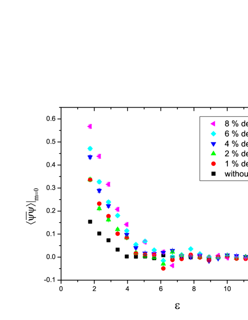
Figure 1: Fig.1. The value of the chiral condensate versus the dielectric permittivity of substrate for the different concentratins of defects.

We generate statistically independent field configuration on $20^{4}$ lattice for different values of dielectric permitttivity $\epsilon$ and percentage of the defects. For each set of lattice parameters we calculate the chiral condensate and conductivity. The dependence of the fermion condensate on the dielectric permittivity substrate at various concentrations defects is shown in Fig.1.

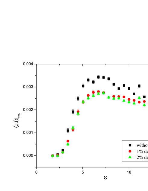
Figure 2: Fig.2. The conductivity of graphene versus the permittivity for different concentrations of defects in the substrate.

Since the ”smeared” conductivity [9] is in direct proportion to the correlator of electromagnetic currents at central point and we are interested in the qualitative dependence of conductivity on the interaction strength and defects concentration, we can study the electromagnetic currents correlator. This dependence is shown in Fig.2.

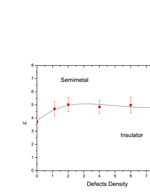
Figure 3: Fig.3. The phase diagram for the semimetal-insulator phase transition in the plane defects density - dielectric permittivity of substrate.

Fig.1 and 2 shows that for certain values of the substrate permittivity the strong change of the conductivity of graphene and the magnitude of the fermion condensate takes place. This change indicates the phase transition, graphene goes from the state of the conductor to the state of the dielectric. Using these data we can plot a phase diagramme in a plane the substrate permittivity - the concentration of defects.

Fig.3 shows a weak dependence of the points of the phase transition on the concentration of defects in the effective field theory.

4 Conclusions

An important conclusion of the analysis is that the presence of defects in the substrate leads to a shift of the phase transition to higher values of the dielectric permittivity. It means that the presence of defects in graphene may facilitate the transition from state of the conductor to the dielectric state.

The authors are grateful to Mikhail Zubkov for interesting and useful discussions. The calculations were performed on a cluster of ITEP “Stakan”, MV 100K at the Moscow Joint Supercomputer Center and at the Supercomputing Center of the Moscow State University.

References

- [1] K. S. Novoselov, A. K. Geim, S. V. Morozov, D. Jiang, Y. Zhang, S. V. Dubonos, I. V. Grigorieva, and A. A. Firsov, Science 306, 666 (2004).
- [2] A. H. Castro Neto, F. Guinea, N. M. R. Peres, K. S. Novoselov, and A. K. Geim, Rev. Mod. Phys. 81, 109 (2009).
- [3] A. K. Geim and K. S. Novoselov, Nature Materials 6, 183 (2007).
- [4] A. S. Mayorov et al., Nano Lett. 12, 4629 (2012).
- [5] M. V. Ulybyshev et al., ArXiv:1304.3660.
- [6] G. W. Semenoff, Phys. Rev. Lett. 53, 2449 (1984).
- [7] J. E. Drut and T. A. Lähde, Phys. Rev. Lett. 102, 026802 (2009); Phys. Rev. B 79, 165425 (2009); Phys. Rev. B 79, 241405 (2009); PoS Lattice2011, 074 (2011); J. E. Drut, T. A. Lähde, and E. Tölö, PoS Lattice2010, 006 (2010).
- [8] S. Hands and C. Strouthos, Phys. Rev. B 78, 165423 (2008); W. Armour, S. Hands, and C. Strouthos, Phys. Rev. B 81, 125105 (2010); Phys. Rev. B 84, 075123 (2011).
- [9] P. V. Buividovich, E. V. Luschevskaya, O. V. Pavlovsky, M. I. Polikarpov and M. V. Ulybyshev, Phys. Rev. B 86 (2012) 045107; P. V. Buividovich and M. I. Polikarpov, Phys. Rev. B 86, 245117 (2012).
- [10] I. Montvay and G. Muenster, Quantum fields on a lattice (Cambridge University Press, 1994).
- [11] T. DeGrand and C. DeTar, Lattice methods for quantum chromodynamics (World Scientific, 2006).
- [12] C. Burden and A. N. Burkitt, Eur. Phys. Lett. 3, 545 (1987).
- [13] P. V. Buividovich, M. N. Chernodub, E. V. Luschevskaya and M. I. Polikarpov, Phys. Lett. B 682, 484 (2010).