OCU-PHYS 389

August, 2013

$2d$-$4d$ Connection between
$q$-Virasoro/$W$ Block at Root of Unity Limit

and
Instanton Partition Function on ALE Space

H. Itoyama^a,b, T. Oota^b and R. Yoshioka^b

^a Department of Mathematics and Physics, Graduate School of Science
Osaka City University

^b Osaka City University Advanced Mathematical Institute (OCAMI)

3-3-138, Sugimoto, Sumiyoshi-ku, Osaka, 558-8585, Japan

Abstract

We propose and demonstrate a limiting procedure in which, starting from the $q$-lifted version (or $K$-theoretic five dimensional version) of the (W)AGT conjecture to be assumed in this paper, the Virasoro/$W$ block is generated in the $r$-th root of unity limit in $q$ in the $2d$ side, while the same limit automatically generates the projection of the five dimensional instanton partition function onto that on the ALE space $\mathbb{R}^{4}/\mathbb{Z}_{r}$. This circumvents case-by-case conjectures to be made in a wealth of examples found so far. In the $2d$ side, we successfully generate the super-Virasoro algebra and the proper screening charge in the $q\rightarrow-1$, $t\rightarrow-1$ limit, from the defining relation of the $q$-Virasoro algebra and the $q$-deformed Heisenberg algebra. The central charge obtained coincides with that of the minimal series carrying odd integers of the $N=1$ superconformal algebra. In the $r$-th root of unity limit in $q$ in the $2d$ side, we give some evidence of the appearance of the parafermion-like currents. Exploiting the $q$-analysis literatures, $q$-deformed $su(n)$ block is readily generated both at generic $q,t$ and the $r$-th root of unity limit. In the $4d$ side, we derive the proper normalization function for general $(n,r)$ that accomplishes the automatic projection through the limit.

1 Introduction

Continuing attention has been paid to the correspondence between the two-dimensional conformal block [1] and the instanton sum [2, 3] identified as the partition function of the four dimensional ${\cal N}=2$ supersymmetric gauge theory. The both sides of this correspondence [4, 5] have already been intensively studied for more than a few years and a wealth of such examples has been found by now. One of the central tools for our study is the $\beta$-deformed matrix model controlling the integral representation of the conformal block [6, 7, 8, 9, 10, 11, 12, 13, 14] and the use [10] of the formula [15, 16] on multiple integrals. This general correspondence, on the other hand, has stayed as conjectures in most of the examples except the few ones [17, 18, 19, 20] and one of the next steps in the developments would be to obtain efficient understanding among these while avoiding making many conjectures.

In this paper, we regard the correspondence between $q$-Virasoro [22, 23, 24, 25, 26, 27]/$W$ block versus five dimensional instanton partition function as a parent one. We propose the following procedure on the orbifolded examples of the correspondence [28, 29, 30, 31, 32, 33, 34, 35, 36, 37]:

1. assume the the $q$-lifted version (or $K$-theoretic five dimensional version) of the (W)AGT conjecture

2. introduce the limiting procedure $q\rightarrow\omega$

3. apply the same limiting procedure to $Z^{{\rm 5d}}_{{\rm inst}}$, which automatically generates the instanton partition function on ALE space.

We emphasize that, through this limiting procedure (and the assumption (1)), the resulting $2d$ conformal block is guaranteed to agree with the corresponding instanton partition function on ALE space.

The limiting procedure we propose in this paper is the following one (Eq. (3.3) in the text):

$$q=\omega\,\mathrm{e}^{-(1/\sqrt{\beta})h},\qquad t=\omega\,\mathrm{e}^{-\sqrt{\beta}h},\qquad p=q/t=\mathrm{e}^{Q_{E}h},$$ (1.1)

with $\omega=\mathrm{e}^{2\pi\mathrm{i}/r}$. We introduce the root of unity limit $q\rightarrow\omega$ by $h\rightarrow+0$ limit. Our procedure is illustrated in Figure 1.

In the next section, we first derive super-Virasoro algebra [38, 39, 40], starting from the defining relation of the $q$-Virasoro algebra and the $q$-deformed Heisenberg algebra [22]. The central charge obtained coincides with that of the minimal series [38] carrying odd integers of the $N=1$ superconformal algebra.

In section three, we consider the $r$-th root of unity limit of $q$ and $t$ for the $q$-Virasoro algebra, and we give some evidence of the appearance of the parafermion-like currents.

In section four, exploiting the $q$-analysis literatures [41, 42, 43, 15, 16], we introduce integral representation of $q$-deformed $su(n)$ block which is valid both at generic $q,t$ and the $r$-th root of unity limit.

In section five, we turn our attention to the $4d$ side. See, for instance, [44, 45, 46, 47, 48, 49]. After some review on the ALE instanton partition function [50], we show that the same limit automatically generates the projection of the five dimensional instanton partition function (see, for instance, [51]) onto that on the ALE space $\mathbb{R}^{4}/\mathbb{Z}_{r}$. We derive the proper normalization function for general $(n,r)$ that accomplishes the automatic projection through the limit.

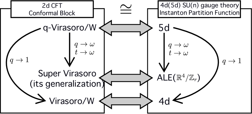
Fig. 1: Illustration of the procedure proposed in this paper.

For M theoretic view point of this correspondence, see, for example, [52]. For recent developments on the connection between $q$-deformed Virasoro algebra and the 5 dimensional partition function on $S^{5}$, see [53].

2 $\bm{q\rightarrow-1}$ limit of $\bm{q}$-Virasoro algebra and $\bm{N=1}$ SCFT

In this section, we consider the $q\rightarrow-1$ limit of the $q$-Virasoro algebra and discuss its connection with the $N=1$ super-Virasoro algebra. This limit corresponds to the $r=2$ case of $q\rightarrow\omega=\mathrm{e}^{2\pi\mathrm{i}/r}$.

2.1 $\bm{q}$-Virasoro algebra for generic $\bm{q}$

The $q$-Virasoro algebra $\mathrm{Vir}_{q,t}$ [22] contains two parameters $q$ and $t$ and has a realization in terms of a $q$-deformed Heisenberg algebra $\mathcal{H}_{q,t}$:

$$\begin{split}[\alpha_{n},\alpha_{m}]&=-\frac{1}{n}\frac{(1-q^{n})(1-t^{-n})}{(1+p^{n})}\delta_{n+m,0},\qquad(n\neq 0),\cr[\alpha_{n},Q]&=\delta_{n,0},\end{split}$$ (2.1)

where $p=q/t$. In terms of these “fundamental bosons”, the generators of the $q$-Virasoro algebra $\mathcal{T}_{n}$ ($n\in\mathbb{Z}$) are realized as

$$\mathcal{T}(z)=:\exp\left(\sum_{n\neq 0}\alpha_{n}z^{-n}\right):p^{1/2}q^{\sqrt{\beta}\alpha_{0}}+:\exp\left(-\sum_{n\neq 0}\alpha_{n}(pz)^{-n}\right):p^{-1/2}q^{-\sqrt{\beta}\alpha_{0}},$$ (2.2)

where $\mathcal{T}(z)=\sum_{n\in\mathbb{Z}}\mathcal{T}_{n}z^{-n}$, and $\beta=\log t/\log q$. Eq. (2.2) satisfies the defining relation of the $q$-Virasoro algebra:

$$f(z^{\prime}/z)\mathcal{T}(z)\mathcal{T}(z^{\prime})-f(z/z^{\prime})\mathcal{T}(z^{\prime})\mathcal{T}(z)=\frac{(1-q)(1-t^{-1})}{(1-p)}\Bigl{[}\delta(pz/z^{\prime})-\delta(p^{-1}z/z^{\prime})\Bigr{]},$$ (2.3)

where

$$f(z)=\exp\left(\sum_{n=1}^{\infty}\frac{1}{n}\frac{(1-q^{n})(1-t^{-n})}{(1+p^{n})}z^{n}\right),$$ (2.4)

and the multiplicative delta function is defined by

$$\delta(z)=\sum_{n\in\mathbb{Z}}z^{n}.$$ (2.5)

Let us introduce two $q$-deformed free bosons by

$$\widetilde{\varphi}^{(\pm)}(z)=\beta^{\pm 1/2}\,Q+2\beta^{\pm 1/2}\alpha_{0}\log z+\sum_{n\neq 0}\frac{(1+p^{-n})}{(1-\xi_{\pm}{}^{n})}\alpha_{n}z^{-n},$$ (2.6)

where $\xi_{+}=q$, $\xi_{-}=t$.

Their correlators are given by

$$\begin{split}\langle\widetilde{\varphi}^{(\pm)}(z_{1})\widetilde{\varphi}^{(\pm)}(z_{2})\rangle&=2\beta^{\pm 1}\log z_{1}-\sum_{n=1}^{\infty}\frac{(1+p^{\pm n})(1-\xi_{\mp}{}^{n})}{n(1-\xi_{\pm}{}^{n})}\left(\frac{z_{2}}{z_{1}}\right)^{n}\cr&=\log\left[z_{1}^{2\beta^{\pm 1}}\left(1-\frac{z_{2}}{z_{1}}\right)\frac{(p^{\pm 1}z_{2}/z_{1};\xi_{\pm})_{\infty}}{(\xi_{\mp}z_{2}/z_{1};\xi_{\pm})_{\infty}}\right],\end{split}$$ (2.7)

$$\langle\widetilde{\varphi}^{(\pm)}(z_{1})\widetilde{\varphi}^{(\mp)}(z_{2})\rangle=\log(z_{1}-z_{2})+\log(z_{1}-p^{\mp 1}z_{2}).$$ (2.8)

Here

$$(x;\xi)_{\infty}=\prod_{k=0}^{\infty}(1-x\,\xi^{k}).$$ (2.9)

Remark. By taking $q\rightarrow 1$ limit with $\beta$ fixed, we have

$$\lim_{q\rightarrow 1}\langle\widetilde{\varphi}^{(\pm)}(z_{1})\widetilde{\varphi}^{(\pm)}(z_{2})\rangle=\log\Bigl{[}(z_{1}-z_{2})^{2\beta^{\pm 1}}\Bigr{]}.$$ (2.10)

Two kinds of deformed screening currents are defined by

$$S_{\pm}(z)=:\mathrm{e}^{\pm\widetilde{\varphi}^{(\pm)}(z)}:.$$ (2.11)

The screening currents $S_{\pm}$ commute with the $q$-Virasoro generators up to total $q$- or $t$-derivative:

$$[\mathcal{T}(z),S_{+}(z^{\prime})]=-(1-q)(1-t^{-1})\frac{\mathrm{d}_{q}}{\mathrm{d}_{q}z^{\prime}}\Bigl{[}\delta(z^{\prime}/z)p^{-1/2}z^{\prime}A_{+}(z^{\prime})\Bigr{]},$$ (2.12)

$$[\mathcal{T}(z),S_{-}(z^{\prime})]=-(1-q^{-1})(1-t)\frac{\mathrm{d}_{t}}{\mathrm{d}_{t}z^{\prime}}\Bigl{[}\delta(z^{\prime}/z)p^{1/2}z^{\prime}A_{-}(z^{\prime})\Bigr{]},$$ (2.13)

where

$$\begin{split}A_{+}(z)&=:\exp\left(\sum_{n\neq 0}\frac{(1+t^{n})}{(1-q^{n})}\alpha_{n}z^{-n}\right):\mathrm{e}^{\sqrt{\beta}Q}q^{-\sqrt{\beta}\alpha_{0}}z^{2\sqrt{\beta}\alpha_{0}},\cr A_{-}(z)&=:\exp\left(-\sum_{n\neq 0}\frac{(1+q^{n})}{(1-t^{n})}\alpha_{n}(pz)^{-n}\right):\mathrm{e}^{-(1/\sqrt{\beta})Q}q^{\sqrt{\beta}\alpha_{0}}z^{-(2/\sqrt{\beta})\alpha_{0}}.\end{split}$$ (2.14)

We use the following convention of the $\xi$-derivative ($\xi=q,t$):

$$\frac{\mathrm{d}_{\xi}}{\mathrm{d}_{\xi}z}f(z)=\frac{f(z)-f(\xi z)}{(1-\xi)z}.$$ (2.15)

Deformed screening charges [26] are defined by the Jackson integral

$$Q^{+}_{[a,b]}=\int_{a}^{b}\mathrm{d}_{q}z\,S_{+}(z),\qquad Q^{-}_{[a,b]}=\int_{a}^{b}\mathrm{d}_{t}z\,S_{-}(z),$$ (2.16)

over a suitably chosen integral domain $[a,b]$.

2.2 $\bm{q\rightarrow-1}$ limit of $\bm{q}$-bosons

First, we consider the $q=-1$ limit of the $q$-bosons (2.6). Let us decompose them into “even” and odd parts:

$$\widetilde{\varphi}^{(\pm)}(z)=\widetilde{\varphi}^{(\pm)}_{\mathrm{even}}(z)+\widetilde{\varphi}^{(\pm)}_{\mathrm{odd}}(z),$$ (2.17)

where

$$\begin{split}\widetilde{\varphi}_{\mathrm{even}}^{(\pm)}(z)&:=\beta^{\pm 1/2}Q+\beta^{\pm 1/2}\alpha_{0}\log(z^{2})+\sum_{n\neq 0}\frac{1+p^{-2n}}{1-\xi_{\pm}{}^{2n}}\alpha_{2n}z^{-2n},\cr\widetilde{\varphi}_{\mathrm{odd}}^{(\pm)}(z)&:=\sum_{n\in\mathbb{Z}}\frac{1+p^{-2n-1}}{1-\xi_{\pm}{}^{2n+1}}\alpha_{2n+1}z^{-2n-1}.\end{split}$$ (2.18)

Note that

$$\widetilde{\varphi}_{\mathrm{even}}^{(\pm)}(\mathrm{e}^{\pi\mathrm{i}}z)=\widetilde{\varphi}_{\mathrm{even}}^{(\pm)}(z)+2\pi\mathrm{i}\,\beta^{\pm 1/2}\,\alpha_{0},\qquad\widetilde{\varphi}_{\mathrm{odd}}^{(\pm)}(-z)=-\widetilde{\varphi}_{\mathrm{odd}}^{(\pm)}(z).$$ (2.19)

Now we consider a $q\rightarrow-1$ limit. Simultaneously, $t\rightarrow-1$ limit is taken. In the remaining part of this section, we assume that $\beta$ takes the following rational value:

$$\beta=\frac{k_{-}+1/2}{k_{+}+1/2}=\frac{2k_{-}+1}{2k_{+}+1},$$ (2.20)

where $k_{\pm}$ are non-negative integers. To make the limit definite, we choose the branch of logarithms of $q$ and $t$ as

$$\log q=2\pi\mathrm{i}(k_{+}+1/2)-\frac{h}{\sqrt{\beta}},\qquad\log t=\beta\log q=2\pi\mathrm{i}(k_{-}+1/2)-\sqrt{\beta}h,$$ (2.21)

with $h>0$. Also,

$$\log p=\log q-\log t=2\pi\mathrm{i}(k_{+}-k_{-})+Q_{E}h.$$ (2.22)

Here $Q_{E}=\sqrt{\beta}-1/\sqrt{\beta}$. Hence

$$q=-\mathrm{e}^{-(1/\sqrt{\beta})h},\qquad t=-\mathrm{e}^{-\sqrt{\beta}h},\qquad p=q/t=\mathrm{e}^{Q_{E}h}.$$ (2.23)

The $q\rightarrow-1$ limit implies $h\rightarrow+0$ limit.

We postulate the following limit of the boson oscillators:

$$\begin{split}\alpha_{2n}&=-\frac{p^{n}}{|n|}\sqrt{-\frac{(1-q^{2n})(1-t^{-2n})}{2(1+p^{2n})}}a_{n}=-h\,a_{n}+O(h^{2}),\qquad(n\neq 0),\cr\alpha_{0}&=a_{0},\cr\alpha_{2n+1}&=\frac{1}{n+1/2}\sqrt{\frac{(1-q^{2n+1})(1-t^{-(2n+1)})}{2(1+p^{-(2n+1)})}}\,\tilde{a}_{n+1/2}\cr&=\frac{1}{n+1/2}\,\tilde{a}_{n+1/2}+Q_{E}\,h\,\tilde{a}_{n+1/2}+O(h^{2}).\end{split}$$ (2.24)

This leads to the following standard commutation relations of boson and twisted boson oscillators:

$$[a_{n},a_{m}]=n\delta_{n+m,0},\qquad[a_{n},Q]=\delta_{n,0},$$ (2.25)

$$[\tilde{a}_{n+1/2},\tilde{a}_{-m-1/2}]=(n+1/2)\delta_{n,m}.$$ (2.26)

Therefore, in the $q\rightarrow-1$ limit of $q$-bosons (2.6), we obtain two free bosons $\phi(w)$ and $\varphi(w)$:

$$\begin{split}\widetilde{\varphi}_{\mathrm{even}}^{(\pm)}(z)&=\beta^{\pm 1/2}\phi(w)+O(h),\cr\widetilde{\varphi}_{\mathrm{odd}}^{(\pm)}(z)&=\varphi(w)+O(h),\end{split}$$ (2.27)

where $z=\sqrt{w}$, and

$$\phi(w)=Q+a_{0}\log w-\sum_{n\neq 0}\frac{a_{n}}{n}w^{-n},$$ (2.28)

$$\varphi(w)=\sum_{n\in\mathbb{Z}}\frac{\tilde{a}_{n+1/2}}{n+1/2}w^{-n-1/2}.$$ (2.29)

Here $\phi(w)$ (resp. $\varphi(w)$) is the ordinary (resp. twisted) boson on the $w$-plane:

$$\langle\phi(w_{1})\phi(w_{2})\rangle=\log(w_{1}-w_{2}),\qquad\langle\varphi(w_{1})\varphi(w_{2})\rangle=\log\left(\frac{\sqrt{w_{1}}-\sqrt{w_{2}}}{\sqrt{w_{1}}+\sqrt{w_{2}}}\right).$$ (2.30)

Note that $\phi(\mathrm{e}^{2\pi\mathrm{i}}w)=\phi(w)+2\pi\mathrm{i}\,a_{0}$, $\varphi(\mathrm{e}^{2\pi\mathrm{i}}w)=-\varphi(w)$.

2.3 $\bm{q\rightarrow-1}$ limit of screening currents

Next, we consider the $q\rightarrow-1$ limit of the screening currents (2.11). Using the limit of $q$-bosons (2.27), we easily see that

$$\lim_{q\rightarrow-1}S_{+}(z)=:\mathrm{e}^{\sqrt{\beta}\phi(w)}\mathrm{e}^{\varphi(w)}:,\qquad\lim_{q\rightarrow-1}S_{-}(z)=:\mathrm{e}^{-(1/\sqrt{\beta})\phi(w)}\mathrm{e}^{-\varphi(w)}:,$$ (2.31)

where $z=\sqrt{w}$.

First, we rewrite the vertex operators $:\mathrm{e}^{\pm\varphi(w)}:$. Since the weight $\pm 1$ is in a (one-dimensional) integral lattice $(\pm 1)^{2}=1\in\mathbb{Z}$, we can construct two fermions :

$$\psi(w)\equiv\frac{\mathrm{i}}{2\sqrt{2w}}\Bigl{(}:\mathrm{e}^{\varphi(w)}:-:\mathrm{e}^{-\varphi(w)}:\Bigr{)},\qquad\widehat{\psi}(w)\equiv\frac{1}{2\sqrt{2w}}\Bigl{(}:\mathrm{e}^{\varphi(w)}:+:\mathrm{e}^{-\varphi(w)}:\Bigr{)}.$$ (2.32)

In terms of these fermions, we have the twisted boson/fermion correspondence:

$$:\mathrm{e}^{\pm\varphi(w)}:=\sqrt{2w}\Bigl{(}\widehat{\psi}(w)\mp\mathrm{i}\psi(w)\Bigr{)}.$$ (2.33)

Using the commutation relations (2.26), we can show that these two fermions (2.32) obey the following anti-commutation relations:

$$\begin{split}\{\psi(w_{1}),\psi(w_{2})\}&=\frac{1}{w_{1}}\delta(w_{2}/w_{1}),\cr\{\widehat{\psi}(w_{1}),\widehat{\psi}(w_{2})\}&=\frac{1}{\sqrt{w_{1}w_{2}}}\delta(w_{2}/w_{1}),\cr\{\psi(w_{1}),\widehat{\psi}(w_{2})\}&=0.\end{split}$$ (2.34)

Notice that

$$\psi(\mathrm{e}^{2\pi\mathrm{i}}\,w)=\psi(w),\qquad\widehat{\psi}(\mathrm{e}^{2\pi\mathrm{i}}\,w)=-\widehat{\psi}(w).$$ (2.35)

They admit the following mode expansion on the $w$-plane:

$$\psi(w)=\sum_{r\in\mathbb{Z}+1/2}\psi_{r}\,w^{-r-1/2},\qquad\widehat{\psi}(w)=\sum_{n\in\mathbb{Z}}\widehat{\psi}_{n}\,w^{-n-1/2}.$$ (2.36)

In terms of these modes, the anti-commutation relations (2.34) are rewritten as

$$\{\psi_{r},\psi_{s}\}=\delta_{r+s,0},\qquad\{\widehat{\psi}_{m},\widehat{\psi}_{n}\}=\delta_{m+n,0},\qquad\{\psi_{r},\widehat{\psi}_{m}\}=0.$$ (2.37)

Here $r,s\in\mathbb{Z}+1/2$ and $m,n\in\mathbb{Z}$. Hence, $\psi(w)$ (resp. $\widehat{\psi}(w)$) is an NS fermion (resp. an R fermion) on the $w$-plane.

On the Fock vacuum,

$$\bigl{\langle}0|\psi(w_{1})\psi(w_{2})|0\bigr{\rangle}=\frac{1}{w_{1}-w_{2}},\qquad\bigl{\langle}0|\widehat{\psi}(w_{1})\widehat{\psi}(w_{2})|0\bigr{\rangle}=\frac{1}{2(w_{1}-w_{2})}\left(\sqrt{\frac{w_{1}}{w_{2}}}+\sqrt{\frac{w_{2}}{w_{1}}}\right),$$ (2.38)

and $\bigl{\langle}0|\psi(w_{1})\widehat{\psi}(w_{2})|0\bigr{\rangle}=0$.

Remark. Let $|0^{\prime}\rangle=\sqrt{2}\,\tilde{a}_{-1/2}|0\rangle$. By definition (2.32), $\psi_{r}$ (resp. $\widehat{\psi}_{n}$) is constructed as an infinite sum of terms with odd (resp. even) number of twisted boson oscillators $\{\tilde{a}_{n+1/2}\}$. Hence, the state $|0^{\prime}\rangle$ is not contained in the “Ramond” sub-module $\mathcal{F}_{R}$ of the twisted boson module over the Fock vacuum:

$$|0^{\prime}\rangle\notin\mathcal{F}_{R}=\mathbb{C}[\widehat{\psi}_{-1},\widehat{\psi}_{-2},\dotsm]|0\rangle,\qquad\mathcal{F}_{R}\subset\mathbb{C}[\tilde{a}_{-1/2},\tilde{a}_{-3/2},\dotsc]|0\rangle.$$ (2.39)

But the state $|0^{\prime}\rangle$ can be obtained by the action of the NS fermion: $\psi_{-1/2}|0\rangle=-\mathrm{i}\,|0^{\prime}\rangle$. Moreover, we have the following isomorphism between twisted boson module and NS and R fermion module:

$$\mathbb{C}[\psi_{-1/2},\psi_{-3/2},\dotsm,\widehat{\psi}_{-1},\widehat{\psi}_{-2},\dotsm]|0\rangle=\mathbb{C}[\tilde{a}_{-1/2},\tilde{a}_{-3/2},\dotsm]|0\rangle.$$ (2.40)

One can show that

$$\widehat{\psi}_{0}|0\rangle=\frac{1}{\sqrt{2}}|0\rangle,\qquad\widehat{\psi}_{0}|0^{\prime}\rangle=-\frac{1}{\sqrt{2}}|0^{\prime}\rangle,$$ (2.41)

$$\langle 0^{\prime}|\widehat{\psi}(w_{1})\widehat{\psi}(w_{2})|0^{\prime}\rangle=\frac{1}{2(w_{1}-w_{2})}\left(\sqrt{\frac{w_{1}}{w_{2}}}+\sqrt{\frac{w_{2}}{w_{1}}}\right),$$ (2.42)

where $\langle 0^{\prime}|=\sqrt{2}\,\langle 0|\tilde{a}_{1/2}$.

2.4 $\bm{q=-1}$ limit of $\bm{q}$-Virasoro generators

In this subsection, we consider the $q\rightarrow-1$ limit of the generating function $\mathcal{T}(z)$ of the $q$-Virasoro generators (2.2). It behaves in this limit as

$$\begin{split}&(-1)^{k_{+}-k_{-}}\mathcal{T}(z)\cr&=\,\,\sqrt{2}\,\mathrm{e}^{2\pi\mathrm{i}\sqrt{\beta}(k_{+}+1/2)a_{0}}\Bigl{[}w^{1/2}\bigl{(}\widehat{\psi}(w)-\mathrm{i}\psi(w)\bigr{)}-h\,w^{3/2}\Bigl{(}\widehat{G}(w)-\mathrm{i}\,G(w)\Bigr{)}\Bigr{]}\cr&+\sqrt{2}\,\mathrm{e}^{-2\pi\mathrm{i}\sqrt{\beta}(k_{+}+1/2)a_{0}}\Bigl{[}w^{1/2}\bigl{(}\widehat{\psi}(w)+\mathrm{i}\psi(w)\bigr{)}+h\,w^{3/2}\Bigl{(}\widehat{G}(w)+\mathrm{i}\,G(w)\Bigr{)}\Bigr{]}+O(h^{2})\cr&=2\sqrt{2}\,\cos\bigl{(}2\pi\sqrt{\beta}(k_{+}+1/2)a_{0}\bigr{)}\Bigl{(}w^{1/2}\widehat{\psi}(w)+\mathrm{i}\,h\,w^{3/2}\,G(w)\Bigr{)}\cr&\ +2\sqrt{2}\,\sin\bigl{(}2\pi\sqrt{\beta}(k_{+}+1/2)a_{0}\bigr{)}\Bigl{(}w^{1/2}\psi(w)-\mathrm{i}\,h\,w^{3/2}\,\widehat{G}(w)\Bigr{)}+O(h^{2}),\end{split}$$ (2.43)

where

$$\begin{split}G(w)&=\psi(w)\partial\phi(w)+Q_{E}\,\partial\psi(w),\cr\widehat{G}(w)&=\widehat{\psi}(w)\partial\phi(w)+Q_{E}\,\partial\widehat{\psi}(w).\end{split}$$ (2.44)

Let

$$T(w)=\frac{1}{2}:\bigl{(}\partial\phi(w)\bigr{)}^{2}:+\frac{Q_{E}}{2}\partial^{2}\phi(w)-\frac{1}{2}:\psi(w)\partial\psi(w):.$$ (2.45)

Then, $T(w)$ and $G(w)$ obey the $N=1$ superconformal algebra in the NS sector:

$$\begin{split}T(w_{1})T(w_{2})&=\frac{(3/4)\hat{c}}{(w_{1}-w_{2})^{4}}+\frac{2\,T(w_{2})}{(w_{1}-w_{2})^{2}}+\frac{T^{\prime}(w_{2})}{w_{1}-w_{2}}+\dotsm,\cr T(w_{1})G(w_{2})&=\frac{(3/2)G(w_{2})}{(w_{1}-w_{2})^{2}}+\frac{G^{\prime}(w_{2})}{w_{1}-w_{2}}+\dotsm,\cr G(w_{1})G(w_{2})&=\frac{\hat{c}}{(w_{1}-w_{2})^{3}}+\frac{2T(w_{2})}{w_{1}-w_{2}}+\dotsm,\end{split}$$ (2.46)

where

$$\hat{c}=1-2Q_{E}^{2}=1-2\left(\sqrt{\beta}-\frac{1}{\sqrt{\beta}}\right)^{2}=1-\frac{8(k_{-}-k_{+})^{2}}{(2k_{+}+1)(2k_{-}+1)}.$$ (2.47)

After replacing $\psi(w)$ with $\widehat{\psi}(w)$ in (2.45), $T(w)$ and $\widehat{G}(w)$ obey the $N=1$ algebra in the R sector.

Recall that the $N=1$ minimal superconformal models have the central charge

$$\hat{c}=1-\frac{2(m^{\prime}-m)^{2}}{mm^{\prime}}.$$ (2.48)

Therefore, $\hat{c}$ (2.47) corresponds to an $N=1$ minimal model such that $m$ and $m^{\prime}$ are both positive odd integers: $m=2k_{+}+1$ and $m^{\prime}=2k_{-}+1$. Without loss of generality, we can take $m^{\prime}>m$, i.e., $k_{-}>k_{+}$. The unitary minimal models [38] occur when $k_{-}=k_{+}+1$ and $k_{+}\geq 1$.

2.5 Vertex operator and its $\bm{q\rightarrow-1}$ limit

Let us choose a $q$-deformed Vertex operator $V_{\alpha}(z)$ as

$$V_{\alpha}(z)=:\mathrm{e}^{\Phi_{\alpha}(z)}:,$$ (2.49)

where

$$\Phi_{\alpha}(z)=\alpha\,Q+2\alpha\,\alpha_{0}\log z+\sum_{n\neq 0}\frac{q^{-n}(1-q^{2\sqrt{\beta}\alpha|n|})}{(1-q^{-|n|})(1-t^{-n})}\alpha_{n}z^{-n}.$$ (2.50)

The correlator of this $q$-boson with $\widetilde{\varphi}^{(+)}$ is given by

$$\begin{split}\langle\Phi_{\alpha}(z_{1})\widetilde{\varphi}^{(+)}(z_{2})\rangle=\langle\widetilde{\varphi}^{(+)}(z_{1})\Phi_{\alpha}(z_{2})\rangle&=2\sqrt{\beta}\,\alpha\log z_{1}-\sum_{n=1}^{\infty}\frac{1}{n}\frac{(1-q^{2\sqrt{\beta}\alpha n})}{(1-q^{n})}\left(\frac{qz_{2}}{z_{1}}\right)^{n}\cr&=\log\left[z^{2\sqrt{\beta}\alpha}\frac{(qz_{2}/z_{1};q)_{\infty}}{(q^{1+2\sqrt{\beta}\alpha}z_{2}/z_{1};q)_{\infty}}\right].\end{split}$$ (2.51)

The correlator among themselves is given by

$$\langle\Phi_{\alpha}(z_{1})\Phi_{\alpha^{\prime}}(z_{2})\rangle=2\alpha\alpha^{\prime}\log z_{1}-\sum_{n=1}^{\infty}\frac{1}{n}\frac{(1-q^{2\sqrt{\beta}\alpha n})(1-q^{2\sqrt{\beta}\alpha^{\prime}n})}{(1-q^{n})(1-t^{n})(1+p^{n})}\left(\frac{q^{2}z_{2}}{z_{1}}\right)^{n}.$$ (2.52)

We restrict the parameter $\alpha$ to take values corresponding to those of the primary fields of the minimal theories in the NS sector:

$$\alpha=\alpha_{r,s}=-\left(\frac{1-r}{2}\right)\frac{1}{\sqrt{\beta}}+\left(\frac{1-s}{2}\right)\sqrt{\beta},$$ (2.53)

where

$$1\leq r\leq 2k_{-},\qquad 1\leq s\leq 2k_{+},\qquad r-s\in 2\mathbb{Z}.$$ (2.54)

Then

$$L_{r,s}\equiv(2k_{+}+1)\sqrt{\beta}\alpha_{r,s}=-k_{+}(1-r)+(1-s)k_{-}+\left(\frac{r-s}{2}\right)\in\mathbb{Z}.$$ (2.55)

We can see that

$$\lim_{q\rightarrow-1}\Phi_{\alpha_{r,s}}(z)=\alpha_{r,s}\phi(w)-\frac{1}{4}\Bigl{(}1-(-1)^{L_{r,s}}\Bigr{)}\varphi(w).$$ (2.56)

Therefore, the $q\rightarrow-1$ limit of the deformed vertex operator (2.49) is given by

$$\lim_{q\rightarrow-1}V_{\alpha_{r,s}}(z)=\begin{cases}:\mathrm{e}^{\alpha_{r,s}\phi(w)}:&\ \ \ \mbox{for $L_{r,s}$ even},\cr:\mathrm{e}^{\alpha_{r,s}\phi(w)}\mathrm{e}^{-(1/2)\varphi(w)}:&\ \ \ \mbox{for $L_{r,s}$ odd}.\end{cases}$$ (2.57)

For $L_{r,s}$ even, $:\mathrm{e}^{\alpha_{r,s}(w)}:$ is exactly equal to the Coulomb gas representation of the bosonic primary field in the NS sector with scaling dimension

$$\Delta_{\alpha_{r,s}}=\frac{1}{2}\alpha_{r,s}(\alpha_{r,s}-Q_{E})=-\frac{1}{8}Q_{E}^{2}+\frac{1}{8}\left(-\frac{r}{\sqrt{\beta}}+s\sqrt{\beta}\right)^{2}.$$ (2.58)

For $L_{r,s}$ odd, the interpretation of the vertex operator $:\mathrm{e}^{-(1/2)\varphi(w)}:$ is unclear. The operator product expansion of the vertex operators $:\mathrm{e}^{\pm(1/2)\varphi(w)}:$ with the NS fermion is given by

$$\psi(w_{1}):\mathrm{e}^{\pm(1/2)\varphi(w_{2})}:=\mp\frac{\mathrm{i}}{\sqrt{2}(w_{1}-w_{2})^{1/2}}:\mathrm{e}^{\mp(1/2)\varphi(w_{2})}:+\dotsm,$$ (2.59)

which is similar to those of the spin fields, but they do not affect the Fock vacuum:

$$:\mathrm{e}^{\pm(1/2)\varphi(0)}:|0\rangle=|0\rangle.$$ (2.60)

Hence, these are not spin fields. In the remaining part of this section, we only consider the case of $L_{r,s}$ even.

Next, let us consider the $q\rightarrow-1$ limit of the Jackson integral

$$\int_{0}^{a}\mathrm{d}_{q}z\,f(z)=a(1-q)\sum_{k=0}^{\infty}f(aq^{k})q^{k}.$$ (2.61)

For $q=-\mathrm{e}^{-h}$ and $f(z)=\sum_{n=0}^{\infty}f_{n}z^{n}$, we can show that

$$\lim_{h\rightarrow 0}(1+q)\int_{0}^{a}\mathrm{d}_{q}z\,f(z)=\int_{0}^{a}\bigl{(}f(z)-f(-z)\bigr{)}\mathrm{d}z=\int_{0}^{a}\left(\frac{f(z)-f(-z)}{z}\right)z\mathrm{d}z=\int_{0}^{a^{2}}g(w)\mathrm{d}w.$$ (2.62)

Here $w=z^{2}$ and

$$g(w):=\frac{f(z)-f(-z)}{2z}.$$ (2.63)

We propose the following “limit” of the $q$-screening charge $Q_{[a,b]}^{+}$ for the rational $\beta$ (2.20):

$$\begin{split}&\frac{\mathrm{i}}{\sqrt{2}}(1+q)Q^{+}_{[a,b]}=\frac{\mathrm{i}}{\sqrt{2}}(1+q)\int_{a}^{b}\mathrm{d}_{q}z\,:\mathrm{e}^{\widetilde{\varphi}_{\mathrm{odd}}(z)}:\,:\mathrm{e}^{\widetilde{\varphi}_{\mathrm{even}}(z)}:\cr&\longrightarrow\frac{\mathrm{i}}{\sqrt{2}}\int_{a}^{b}\mathrm{d}z\,z\left(\frac{:\mathrm{e}^{\varphi(z)}:-:\mathrm{e}^{-\varphi(z)}:}{z}\right):\mathrm{e}^{\sqrt{\beta}\phi(z^{2})}:\equiv Q_{[a^{2},b^{2}]}^{(+)},\end{split}$$ (2.64)

where

$$Q_{[a^{2},b^{2}]}^{(+)}=\int_{a^{2}}^{b^{2}}\mathrm{d}w\,\psi(w):\mathrm{e}^{\sqrt{\beta}\phi(w)}:.$$ (2.65)

Here we have ignored the subtlety due to the zero-mode and negative power terms. To be more precise, the “limit” (2.64) includes a kind of projection imposed by hand. Note that

$$\lim_{h\rightarrow 0}:\mathrm{e}^{\widetilde{\varphi}_{\mathrm{odd}}(z)}:=:\mathrm{e}^{\varphi(z)}:=\sqrt{2}z\left(\widehat{\psi}(w)-\mathrm{i}\psi(w)\right).$$ (2.66)

Hence this projection is equivalent to drop the R fermion $\widehat{\psi}(w)$. We see that the resulting screening charge (2.65) is the screening charge for the superconformal block [55, 56].

3 Root of unity limit of $\bm{q}$-Virasoro algebra and parafermion-like structure

In this section, we consider the $r$-th root of unity limit of the $q$-Virasoro algebra. In particular, we show that the screening currents $S_{\pm}$ in the limit are closely related to parafermion-like currents.

The parafermion currents are introduced in [57]. The partition functions of the parafermionic theories are studied in [58]. For recent work which discuss the connection between parafermions and Selberg integrals, see [59].

We assume that $\beta$ takes the following rational value:

$$\beta=\frac{k_{-}+1/r}{k_{+}+1/r}=\frac{rk_{-}+1}{rk_{+}+1},$$ (3.1)

where $k_{\pm}$ are non-negative integers and choose the branch of logarithms of $q$ and $t$ as

$$\log q=2\pi\mathrm{i}(k_{+}+1/r)-\frac{h}{\sqrt{\beta}},\qquad\log t=\beta\log q=2\pi\mathrm{i}(k_{-}+1/r)-\sqrt{\beta}h,$$ (3.2)

with $h>0$. Hence

$$q=\mathrm{e}^{2\pi\mathrm{i}/r}\,\mathrm{e}^{-(1/\sqrt{\beta})h},\qquad t=\mathrm{e}^{2\pi\mathrm{i}/r}\,\mathrm{e}^{-\sqrt{\beta}h},\qquad p=q/t=\mathrm{e}^{Q_{E}h}.$$ (3.3)

The root of unity limit $q\rightarrow\mathrm{e}^{2\pi\mathrm{i}/r}$ implies $h\rightarrow+0$ limit. The $q\rightarrow-1$ limit in the previous section corresponds to the $r=2$ case.

3.1 $q\rightarrow\mathrm{e}^{2\pi\mathrm{i}/r}$ limit of $q$-bosons

Let us decompose the $q$-deformed free bosons (2.6) into two parts:

$$\widetilde{\varphi}^{(\pm)}(z)=\widetilde{\varphi}^{(\pm)}_{0}(z)+\widetilde{\varphi}^{(\pm)}_{R}(z),$$ (3.4)

where

$$\begin{split}\widetilde{\varphi}^{(\pm)}_{0}(z)&=\beta^{\pm 1/2}Q+\frac{2}{r}\beta^{\pm 1/2}\alpha_{0}\log z^{r}+\sum_{n\neq 0}\frac{(1+p^{-nr})}{(1-\xi_{\pm}^{nr})}\alpha_{nr}\,z^{-nr},\cr\widetilde{\varphi}^{(\pm)}_{R}(z)&=\sum_{\ell=1}^{r-1}\sum_{n\in\mathbb{Z}}\frac{(1+p^{-nr-\ell})}{1-\xi_{\pm}^{nr+\ell}}\alpha_{nr+\ell}\,z^{-nr-\ell}.\end{split}$$ (3.5)

We rescale the oscillators as follows

$$\begin{split}Q&=\sqrt{\frac{2}{r}}\,Q_{0},\cr\alpha_{0}&=\sqrt{\frac{r}{2}}\,a_{0},\cr\alpha_{nr}&=-\sqrt{\frac{r}{2}}\,h\,a_{n}+O(h^{2}),\qquad(n\neq 0)\cr\alpha_{nr+\ell}&=\sqrt{\frac{2}{r}}\frac{(1-\mathrm{e}^{2\pi\mathrm{i}(nr+\ell)/r})}{2(n+\ell/r)}\tilde{a}_{n+\ell/r}+O(h),\qquad\qquad(\ell=1,2,\dotsc,r-1).\end{split}$$ (3.6)

The rescaled oscillators obey the following commutation relations

$$[a_{m},a_{n}]=m\delta_{m+n,0},\qquad[a_{n},Q_{0}]=\delta_{n,0},$$ (3.7)

$$[\tilde{a}_{n+\ell/r},\tilde{a}_{-m-\ell^{\prime}/r}]=(n+\ell/r)\delta_{m,n}\delta_{\ell,\ell^{\prime}}.$$ (3.8)

In the $q\rightarrow\mathrm{e}^{2\pi\mathrm{i}/r}$ limit, we have

$$\begin{split}\lim_{h\rightarrow+0}\widetilde{\varphi}_{0}^{(\pm)}(z)&=\sqrt{\frac{2}{r}}\,\beta^{\pm 1/2}\phi(w),\cr\lim_{h\rightarrow+0}\widetilde{\varphi}^{(\pm)}_{R}(z)&=\sqrt{\frac{2}{r}}\,\varphi(w),\end{split}$$ (3.9)

where $w=z^{r}$ and

$$\phi(w)=Q_{0}+a_{0}\log w-\sum_{n\neq 0}\frac{a_{n}}{n}w^{-n},$$ (3.10)

$$\varphi(w)=\sum_{\ell=1}^{r-1}\varphi^{(\ell)}(w),\qquad\varphi^{(\ell)}(w)=\sum_{n\in\mathbb{Z}}\frac{\tilde{a}_{n+\ell/r}}{n+\ell/r}w^{-n-\ell/r}.$$ (3.11)

The correlation functions are given by

$$\langle\phi(w_{1})\phi(w_{2})\rangle=\log(w_{1}-w_{2}),$$ (3.12)

$$\langle\varphi^{(\ell)}(w_{1})\varphi^{(\ell^{\prime})}(w_{2})\rangle=\delta_{\ell+\ell^{\prime},r}\sum_{k=0}^{r-1}\omega^{-k\ell}\log\left[1-\omega^{k}\left(\frac{w_{2}}{w_{1}}\right)^{1/r}\right].$$ (3.13)

$$\langle\varphi(w_{1})\varphi(w_{2})\rangle=\log\left[\frac{(1-(w_{2}/w_{1})^{1/r})^{r}}{1-(w_{2}/w_{1})}\right]=\log\left[\frac{(w_{1}^{1/r}-w_{2}^{1/r})^{r}}{w_{1}-w_{2}}\right].$$ (3.14)

3.2 $q\rightarrow\mathrm{e}^{2\pi\mathrm{i}/r}$ limit of screening currents

In the $q\rightarrow\mathrm{e}^{2\pi\mathrm{i}/r}$ limit, the screening currents (2.11) turn into

$$\lim_{q\rightarrow\mathrm{e}^{2\pi\mathrm{i}/r}}S_{\pm}(z)=:\exp\left(\pm\sqrt{\frac{2}{r}}\beta^{\pm 1/2}\phi(w)\right):\,:\exp\left(\pm\sqrt{\frac{2}{r}}\varphi(w)\right):.$$ (3.15)

Using the vertex operators $\mathrm{e}^{\pm\sqrt{2/r}\,\varphi(w)}$, we can introduce the following fields

$$\Psi_{\pm}^{(\ell)}(w):=\frac{1}{r^{3/2}w^{1-(1/r)}}\sum_{k=0}^{r-1}\mathrm{e}^{2\pi\mathrm{i}k\ell/r}:\exp\left(\pm\sqrt{\frac{2}{r}}\varphi(\mathrm{e}^{2\pi\mathrm{i}k}w)\right):.$$ (3.16)

Note that $\Psi_{\pm}^{(\ell+r)}=\Psi_{\pm}^{(\ell)}$. Hence we can choose the range of $\ell$ as $\ell=0,1,\dots,r-1$.

These fields have the following periodicity:

$$\Psi^{(\ell)}_{\pm}(\mathrm{e}^{2\pi\mathrm{i}}w)=\mathrm{e}^{-2\pi\mathrm{i}(\ell-r+1)/r}\Psi^{(\ell)}_{\pm}(w).$$ (3.17)

The correlators for these fields are given by

$$\begin{split}&\langle 0|\Psi_{\pm}^{(\ell_{1})}(w_{1})\Psi_{\mp}^{(\ell_{2})}(w_{2})|0\rangle\cr&=\frac{\delta_{\ell_{1}+\ell_{2},r}}{(w_{1}-w_{2})^{2(1-(1/r))}}\left(\frac{w_{2}}{w_{1}}\right)^{(\ell_{1}+1-r)/r}\left[1+\left(\frac{\ell_{1}+1-r}{r}\right)\frac{(w_{1}-w_{2})}{w_{1}}\right],\end{split}$$ (3.18)

$$\begin{split}&\langle 0|\Psi_{\pm}^{(\ell_{1})}(w_{1})\Psi_{\pm}^{(\ell_{2})}(w_{2})|0\rangle\cr&=\frac{1}{r(w_{1}-w_{2})^{2/r}(w_{1}w_{2})^{1-(1/r)}}\left[\delta_{\ell_{1},0}\delta_{\ell_{2},0}w_{1}^{2/r}-2\delta_{\ell_{1},1}\delta_{\ell_{2},r-1}(w_{1}w_{2})^{1/r}+\delta_{\ell_{1},2}\delta_{\ell_{2},r-2}w_{2}^{2/r}\right].\end{split}$$ (3.19)

Note that for $w_{1}\rightarrow w_{2}$,

$$\langle 0|\Psi_{\pm}^{(\ell_{1})}(w_{1})\Psi_{\mp}^{(\ell_{2})}(w_{2})|0\rangle=\frac{\delta_{\ell_{1}+\ell_{2},r}}{(w_{1}-w_{2})^{2(1-(1/r))}}\left\{1+O\Bigl{(}(w_{1}-w_{2})^{2}\Bigr{)}\right\}.$$ (3.20)

These fields $\Psi^{(\ell)}_{\pm}(w)$ are analogue of the parafermion current with scaling dimension $\Delta_{1}=1-(1/r)$.

For example, if we set

$$\Psi(w):=\Psi_{+}^{(1)}(w),\qquad\overline{\Psi}(w):=\Psi_{-}^{(r-1)}(w),$$ (3.21)

they obey (for $r>3$)

$$\langle 0|\overline{\Psi}(w_{1})\Psi(w_{2})|0\rangle=\frac{1}{(w_{1}-w_{2})^{2(1-(1/r))}},$$ (3.22)

$$\langle 0|\Psi(w_{1})\Psi(w_{2})|0\rangle=0,\qquad\langle 0|\overline{\Psi}(w_{1})\overline{\Psi}(w_{2})|0\rangle=0.$$ (3.23)

For $f(z)=\sum_{n=0}^{\infty}f_{n}z^{n}$, the Jackson integral in the $q\rightarrow\mathrm{e}^{2\pi\mathrm{i}/r}$ limit is given by

$$\lim_{h\rightarrow 0}\frac{(1-q^{r})}{(1-q)}\int_{0}^{a}\mathrm{d}_{q}z\,f(z)=\int_{0}^{a^{r}}\mathrm{d}w\,g(w),$$ (3.24)

where

$$g(w)=\frac{1}{rz^{r-1}}\sum_{k=0}^{\infty}\mathrm{e}^{2\pi\mathrm{i}k/r}f(\mathrm{e}^{2\pi\mathrm{i}k/r}z)=\sum_{n=0}^{\infty}f_{nr+r-1}w^{n}.$$ (3.25)

Inspired by this limit of the Jackson integral, it may be useful to consider the following “projection”

$$\frac{1}{\sqrt{r}}\frac{(1-q^{r})}{(1-q)}\int_{a}^{b}\mathrm{d}_{q}z\,S_{+}(z)\longrightarrow Q_{[a^{r},b^{r}]}^{(+)}=\int_{a^{r}}^{b^{r}}\mathrm{d}w\,\Psi(w)\,:\mathrm{e}^{\sqrt{2\beta/r}\,\phi(w)}:,$$ (3.26)

which is a generalization of (2.64).

For the $r=2$ case, $Q_{[a^{2},b^{2}]}^{(+)}$ is the screening charge of the $N=1$ superconformal algebra. Hence $Q_{[a^{r},b^{r}]}^{(+)}$ may play the role of a screening charge for a parafermionic algebra.

4 Review of conformal block and its $\bm{q}$-lift

The $q$-deformed $W_{n}$ algebra is introduced in [60, 24]. The $q$-Virasoro algebra is the $n=2$ case of these series of algebras. For general $n$, the root of unity limit can be studied similarly as in sections 2 and 3. But the analysis of the limit requires a hard task.

The $q$-deformed $W$ algebra at roots of unity itself will not be exploited here for our study of the $q$-lifted version of (W)AGT conjecture. It is the ($q$-deformed) conformal block for the $W_{n}$ algebra which play the key role for the conjecture.

For the conformal block, there is a simple recipe for the $q$-lift ($q$-deformation) without explicitly treating the $q$-$W$ algebra. In subsection 4.1, we review the conformal block of $W_{n}$ algebra written as the Dotsenko-Fateev (DF) multiple integrals. It can be converted into the multiple integrals closely related to the $A_{n-1}$ Selberg integrals. In subsection 4.2, the $q$-lifted conformal block are given. An expansion of the $q$-deformed conformal block in the cross ratio is also mentioned.

The Kadell formula for the Macdonald polynomials is the basic calculational tool of our study [10]. The Kadell formula and their explicit forms for a few Macdonald polynomials are summarized in subsection 4.3.

4.1 Conformal block: From DF to Selberg

Let us consider the conformal field theory with the central charge $c$

$$c=(n-1)\bigl{(}1-n(n+1)Q_{E}^{2}\bigr{)},\qquad Q_{E}=\sqrt{\beta}-\frac{1}{\sqrt{\beta}},$$ (4.1)

associated with the $A_{n-1}=\mathfrak{sl}(n)$ Lie algebra. Let $\mathfrak{h}$ be the Cartan subalgebra of $A_{n-1}$ and $\mathfrak{h}^{*}$ its dual.

The four-point conformal block of the chiral vertex operators can be expressed in terms of free fields. Let $\phi(z)$ be an $\mathfrak{h}$-valued free chiral boson with correlation functions:

$$\begin{split}\langle\phi_{a}(z)\phi_{b}(w)\rangle=(e_{a},e_{b})\log(z-w),~{}~{}~{}\phi_{a}(z)=\langle e_{a},\phi(z)\rangle,\\ e_{a}\in\mathfrak{h}^{*}:~{}\text{a simple root of $A_{n-1}$},~{}~{}~{}a=1,\cdots,n-1.\end{split}$$ (4.2)

Here $(\cdot,\cdot)$ is the symmetric bilinear form on $\mathfrak{h}^{*}$ and $\langle\cdot,\cdot\rangle$ is the natural pairing between $\mathfrak{h}^{*}$ and $\mathfrak{h}$. With $(e_{a},e_{a})=2$, $C_{ab}:=(e_{a},e_{b})$ is the Cartan matrix of the $A_{n-1}$ algebra. The corresponding energy-momentum tensor $T(z)$ is given by

$$\begin{split}T(z)&=\frac{1}{2}:\mathcal{K}\bigl{(}\partial\phi(z),\partial\phi(z)\bigr{)}:+Q_{E}\langle\rho,\partial^{2}\phi(z)\rangle\cr&=\sum_{a,b=1}^{n-1}(C^{-1})^{ab}\left(\frac{1}{2}:\partial\phi_{a}(z)\partial\phi_{b}(z):+Q_{E}\partial^{2}\phi_{b}(z)\right).\end{split}$$ (4.3)

Here $\mathcal{K}(\cdot,\cdot)$ is the Killing form and $\rho$ is the half the sum of positive roots of the $A_{n-1}$ algebra:

$$\rho=\frac{1}{2}\sum_{a=1}^{n-1}a(n-a)e_{a}.$$ (4.4)

The scaling dimension of the vertex operator $V_{\alpha}(z)=:\mathrm{e}^{\langle\alpha,\phi(z)\rangle}:$ $(\alpha\in\mathfrak{h}^{*})$ is given by

$$\frac{1}{2}(\alpha,\alpha)-Q_{E}(\rho,\alpha).$$ (4.5)

The free-field representation of the conformal block is then given by

$$\begin{split}&\mathcal{F}(c,\Delta_{I},\Delta_{i}|\Lambda)\cr&=\biggl{\langle}V_{(1/\sqrt{\beta})\alpha_{1}}(0)V_{(1/\sqrt{\beta})\alpha_{2}}(\Lambda)V_{(1/\sqrt{\beta})\alpha_{3}}(1)V_{(1/\sqrt{\beta})\alpha_{4}}(\infty)\prod_{a=1}^{n-1}\mathcal{Q}_{a}{}^{N_{a}}\widetilde{\mathcal{Q}}_{a}{}^{\widetilde{N}_{a}}\biggl{\rangle},\end{split}$$ (4.6)

with $\alpha_{i}\in\mathfrak{h}^{*}$ $(i=1,2,3,4)$. Two kinds of screening charges are inserted:

$$\mathcal{Q}_{a}=\int_{0}^{\Lambda}\mathrm{d}z\,V_{\sqrt{\beta}e_{a}}(z),\qquad\widetilde{\mathcal{Q}}_{a}=\int_{1}^{\infty}\mathrm{d}z\,V_{\sqrt{\beta}e_{a}}(z).$$ (4.7)

The four points are set to $z_{1}=0$, $z_{2}=\Lambda$, $z_{3}=1$, $z_{4}=\infty$. Hence $\Lambda$ is the cross ratio. The central charge $c$ is given by (4.1), the scaling dimensions $\Delta_{i}$ of the external states are given by

$$\Delta_{i}=\frac{1}{2\beta}(\alpha_{i},\alpha_{i})-\left(1-\frac{1}{\beta}\right)(\rho,\alpha_{i}),\qquad(i=1,2,3,4),$$ (4.8)

and the scaling dimension $\Delta_{I}$ of the intermediate state is given by

$$\Delta_{I}=\frac{1}{2\beta}(\alpha_{I},\alpha_{I})-\left(1-\frac{1}{\beta}\right)(\rho,\alpha_{I}),$$ (4.9)

with

$$\alpha_{I}:=\alpha_{1}+\alpha_{2}+\beta\sum_{a=1}^{n-1}N_{a}e_{a}=-(\alpha_{3}+\alpha_{4})-\beta\sum_{a=1}^{n-1}\widetilde{N}_{a}e_{a}+2(\beta-1)\rho.$$ (4.10)

Here we have used the momentum conservation condition:

$$\frac{1}{\sqrt{\beta}}(\alpha_{1}+\alpha_{2}+\alpha_{3}+\alpha_{4})+\sqrt{\beta}\sum_{a=1}^{n-1}(N_{a}+\widetilde{N}_{a})e_{a}-2Q_{E}\,\rho=0.$$ (4.11)

By using the Wick’s theorem, we obtain the Dotsenko-Fateev integral representation of the conformal block (LABEL:ZDF) [61]

$$\begin{split}\mathcal{F}&=\Lambda^{(\alpha_{1},\alpha_{2})/\beta}(1-\Lambda)^{(\alpha_{2},\alpha_{3})/\beta}\cr&\qquad\times\int\mathrm{d}z\Bigl{(}\Delta_{A_{n-1}}(z)\Bigr{)}^{\beta}\prod_{I=1}^{N_{a}+\widetilde{N}_{a}}(z_{I}^{(a)})^{(\alpha_{1},e_{a})}|z_{I}^{(a)}-\Lambda|^{(\alpha_{2},e_{a})}|z_{I}^{(a)}-1|^{(\alpha_{3},e_{a})},\end{split}$$ (4.12)

where

$$\int\mathrm{d}z=\prod_{a=1}^{n-1}\left\{\prod_{I=1}^{N_{a}}\int_{0}^{\Lambda}\mathrm{d}z_{I}^{(a)}\prod_{J=N_{a}+1}^{N_{a}+\widetilde{N}_{a}}\int_{1}^{\infty}\mathrm{d}z_{J}^{(a)}\right\},$$ (4.13)

$$\Delta_{A_{n-1}}(z)=\prod_{a=1}^{n-1}\prod_{I<J}^{N_{a}+\widetilde{N}_{a}}|z_{J}^{(a)}-z_{I}^{(a)}|^{2}\,\prod_{b=1}^{n-2}\prod_{I=1}^{N_{b}+\widetilde{N}_{b}}\prod_{J=1}^{N_{b+1}+\widetilde{N}_{b+1}}|z_{J}^{(b+1)}-z_{I}^{(b)}|^{-1}.$$ (4.14)

By changing the integration variables from $z_{I}^{(a)}$ ($I=1,2,\dotsc,N_{a}+\widetilde{N}_{a}$) to $x_{I}^{(a)}$ ($I=1,2,\dotsc,N_{a}$) and $y_{J}^{(a)}$ $(J=1,2,\dotsc,\widetilde{N}_{a})$, defined by

$$\Lambda x_{I}^{(a)}:=z_{I}^{(a)},~{}~{}~{}~{}\frac{1}{y_{J}^{(a)}}:=z_{N_{a}+J}^{(a)},$$ (4.15)

we obtain the following Selberg-type multiple integral [10]:

$$\mathcal{F}=\Lambda^{\Delta_{I}-\Delta_{1}-\Delta_{2}}(1-\Lambda)^{(\alpha_{2},\alpha_{3})/\beta}Z_{S}(\Lambda),$$ (4.16)

where

$$\begin{split}Z_{S}(\Lambda)&:=\int_{[0,1]^{N}}\mathrm{d}x\,\Bigl{(}\Delta_{A_{n-1}}(x)\Bigr{)}^{\beta}\prod_{a=1}^{n-1}\prod_{I=1}^{N_{a}}(x_{I}^{(a)})^{(\alpha_{1},e_{a})}(1-x_{I}^{(a)})^{(\alpha_{2},e_{a})}\cr&\qquad\times\int_{[0,1]^{\widetilde{N}}}\mathrm{d}y\,\Bigl{(}\Delta_{A_{n-1}}(y)\Bigr{)}^{\beta}\prod_{b=1}^{n-1}\prod_{J=1}^{N_{b}}(y_{J}^{(b)})^{(\alpha_{4},e_{b})}(1-y_{J}^{(b)})^{(\alpha_{3},e_{b})}\,F(x,y|\Lambda).\end{split}$$ (4.17)

Here $N:=\sum_{a}N_{a}$, $\widetilde{N}:=\sum_{a}\widetilde{N}_{a}$,

$$F(x,y|\Lambda):=\prod_{a=1}^{n-1}\left\{\prod_{I=1}^{N_{a}}(1-\Lambda x_{I}^{(a)})^{(\alpha_{3},e_{a})}\prod_{J=1}^{\widetilde{N}_{a}}(1-\Lambda y_{J}^{(a)})^{(\alpha_{2},e_{a})}\right\}\prod_{a=1}^{n-1}\prod_{b=1}^{n-1}\prod_{I=1}^{N_{a}}\prod_{J=1}^{\widetilde{N}_{b}}(1-\Lambda x_{I}^{(a)}y_{J}^{(b)})^{\beta C_{ab}},$$ (4.18)

$$\mathrm{d}x=\prod_{a=1}^{n-1}\prod_{I=1}^{N_{a}}\mathrm{d}x_{I}^{(a)},\qquad\mathrm{d}y=\prod_{a=1}^{n-1}\prod_{J=1}^{\widetilde{N}_{a}}\mathrm{d}y_{J}^{(a)},$$ (4.19)

$$\Delta_{A_{n-1}}(x)=\prod_{a=1}^{n-1}\prod_{I<J}^{N_{a}}|x_{I}^{(a)}-x_{J}^{(a)}|^{2}\prod_{b=1}^{n-2}\prod_{I=1}^{N_{b}}\prod_{J=1}^{N_{b+1}}|x_{J}^{(b+1)}-x_{I}^{(b)}|^{-1},$$ (4.20)

$$\Delta_{A_{n-1}}(y)=\prod_{a=1}^{n-1}\prod_{I<J}^{\widetilde{N}_{a}}|y_{I}^{(a)}-y_{J}^{(a)}|^{2}\prod_{b=1}^{n-2}\prod_{I=1}^{\widetilde{N}_{b}}\prod_{J=1}^{\widetilde{N}_{b+1}}|y_{J}^{(b+1)}-y_{I}^{(b)}|^{-1}.$$ (4.21)

Strictly speaking, in order for the multiple integral (4.17) to be well-defined, the integration domains $[0,1]^{N}$ and $[0,1]^{\widetilde{N}}$ must be deformed properly.

Let us denote the $A_{n-1}$ Selberg integral [43] by

$$\begin{split}&I^{A_{n-1}}_{k_{1},\dotsc,k_{n-1}}(\kappa;\alpha_{1},\dotsc,\alpha_{n-1};\beta)\cr&=\int_{C_{\beta}^{k_{1},\dotsc,k_{n-1}}[0,1]}\mathrm{d}t\,\Bigl{(}\Delta_{A_{n-1}}(t)\Bigr{)}^{\beta}\prod_{a=1}^{n-1}\prod_{I=1}^{k_{a}}(t_{I}^{(a)})^{\kappa_{a}-1}(1-t_{I}^{(a)})^{\alpha_{a}-1},\end{split}$$ (4.22)

where $\kappa_{a}-1=\delta_{a,n-1}(\kappa-1)$,

$$\mathrm{d}t=\prod_{a=1}^{n-1}\prod_{I=1}^{k_{a}}\mathrm{d}t^{(a)}_{I},\qquad\Delta_{A_{n-1}}(t)=\prod_{a=1}^{n-1}\prod_{I<J}^{k_{a}}|t_{I}^{(a)}-t_{J}^{(a)}|^{2}\prod_{b=1}^{n-2}\prod_{I=1}^{k_{b}}\prod_{J=1}^{k_{b+1}}|t_{J}^{(b+1)}-t_{I}^{(b)}|^{-1}.$$ (4.23)

For the definition of properly deformed integration domain $C^{k_{1},\dotsc,k_{n-1}}_{\beta}[0,1]$, see [43]. For

$$0\leq k_{1}\leq n_{2}\leq\dotsm\leq k_{n-1},k_{0}=k_{n}=0,$$

$$\mathrm{Re}(\kappa)>0,\ \ \mathrm{Re}(\alpha_{a})>0\ \ (a=1,2,\dotsc,n-1),\ \ -\mathrm{min}\left\{\frac{\mathrm{Re}(\kappa)}{k_{n-1}-1},\frac{1}{k_{n-1}}\right\}<\mathrm{Re}(\beta)<\frac{1}{k_{n-1}},$$

and

$$-\frac{\mathrm{Re}(\alpha_{a})}{k_{a}-k_{a-1}-1}<\mathrm{Re}(\beta)<\frac{\mathrm{Re}(\alpha_{a}+\dotsm+\alpha_{b})}{b-a},\qquad(1\leq a\leq b\leq n-1),$$

it holds that

$$\begin{split}&I^{A_{n-1}}_{k_{1},\dotsm,k_{n-1}}(\kappa;\alpha_{1},\dotsc,\alpha_{n-1};\beta)\cr&=\prod_{1\leq a\leq b\leq n-1}\prod_{j=1}^{k_{a}-k_{a-1}}\frac{\Gamma(\alpha_{a}+\dotsm+\alpha_{b}+(j+a-b-1)\beta)}{\Gamma(\kappa_{b}+\alpha_{a}+\dotsm+\alpha_{b}+(j+a-b+k_{b}-k_{b+1}-2)\beta)}\cr&\times\prod_{a=1}^{n-1}\prod_{j=1}^{k_{a}}\frac{\Gamma(\kappa_{a}+(j-k_{a+1}-1)\beta)\,\Gamma(j\beta)}{\Gamma(\beta)}.\end{split}$$ (4.24)

We also use the following notation for normalized $A_{n-1}$ Selberg integral

$$S^{A_{n-1}}_{k_{1},\dotsc,k_{n-1}}(\kappa;\alpha_{1},\dotsc,\alpha_{n-1};\beta):=\frac{1}{\mathrm{vol}(C^{k_{1},\dotsc,k_{n-1}}_{\beta}[0,1])}I^{A_{n-1}}_{k_{1},\dotsc,k_{n-1}}(\kappa;\alpha_{1},\dotsc,\alpha_{n-1};\beta),$$ (4.25)

where

$$\mathrm{vol}(C^{k_{1},\dotsc,k_{n-1}}_{\beta}[0,1])=\int_{C^{k_{1},\dotsc,k_{n-1}}_{\beta}[0,1]}\mathrm{d}t.$$ (4.26)

Let $\omega_{a}$ be the fundamental weights: $(\omega_{a},e_{b}^{\vee})=\delta_{ab}$. Here $e_{b}^{\vee}=2e_{b}/(e_{b},e_{b})=e_{b}$ are the simple coroots. We choose two external momenta $\alpha_{1}$ and $\alpha_{4}$ to be proportional to $\omega_{n-1}$:

$$\alpha_{1}=u_{+}\,\omega_{n-1},\qquad\alpha_{4}=u_{-}\,\omega_{n-1}.$$ (4.27)

Note that in the integrand of (4.17), only the polynomial $F(x,y|\Lambda)$ (4.18) has dependence on the cross ratio $\Lambda$. With the conditions (4.27), $Z_{S}$ factorizes into product of two $A_{n-1}$ Selberg integrals at $\Lambda=0$:

$$\begin{split}Z_{S}(0)&=S^{A_{n-1}}_{N_{1},\dotsc,N_{n-1}}(1+u_{+};1+v_{1+},\dotsm,1+v_{(n-1)+};\beta)\cr&\times S^{A_{n-1}}_{\widetilde{N}_{1},\dotsc,\widetilde{N}_{n-1}}(1+u_{-};1+v_{1-},\dotsm,1+v_{(n-1)-};\beta),\end{split}$$ (4.28)

where

$$v_{a+}:=(\alpha_{2},e_{a}),\qquad v_{a-}:=(\alpha_{3},e_{a}).$$ (4.29)

Let us rewrite (4.17) as

$$Z_{S}(\Lambda)=Z_{s}(0)\,\Bigl{\langle}\!\!\Bigl{\langle}F(x,y|\Lambda)\Bigr{\rangle}_{+}\Bigr{\rangle}_{-},$$ (4.30)

Here $\langle\dotsm\rangle_{+}$ (resp. $\langle\dotsm\rangle_{-}$) is the average over the $A_{n-1}$ Selberg integral $I^{A_{n-1}}_{N_{1},\dotsc,N_{n-1}}(1+u_{+};\{1+v_{a+}\};\beta)$ (resp. $I^{A_{n-1}}_{\widetilde{N}_{1},\dotsm,\widetilde{N}_{n-1}}(1+u_{-};\{1+v_{a-}\};\beta)$), normalized as $\langle 1\rangle_{\pm}=1$.

The AGT relation implies that $Z_{S}(\Lambda)/Z_{S}(0)$ is equal to the instanton part of the Nekrasov partition function of $\mathcal{N}=2$ $SU(n)$ gauge theory with $N_{f}=2n$ fundamental matters.

4.2 $\bm{q}$-deformed conformal block

In order to study the five-dimensional version of AGT conjecture, we need a $q$-deformed conformal block.

4.2.1 $\bm{q}$-deformation

There is a simple recipe [41, 63] to obtain a $q$-deformation of the Selberg-type multiple integral. For the Selberg integral, defined by

$$S_{n}(\beta_{1},\beta_{2},\beta)=\left(\prod_{I=1}^{n}\int_{0}^{1}\mathrm{d}x_{I}\right)\prod_{I=1}^{n}x_{I}^{\beta_{1}-1}(1-x_{I})^{\beta_{2}-1}\prod_{1\leq I<J\leq n}(x_{I}-x_{J})^{2\beta},$$ (4.31)

replace the integral by the definite $q$-integral

$$\int_{0}^{1}\mathrm{d}x_{I}~{}~{}\to~{}~{}\int_{0}^{1}\mathrm{d}_{q}x_{I},$$ (4.32)

and the following factors by their $q$-deformed counterparts

$$\begin{split}(1-x_{I})^{\beta_{2}-1}~{}~{}&\to~{}~{}\prod_{k=0}^{\beta_{2}-1}(1-q^{k}x_{I}),\cr\prod_{1\leq I<J\leq n}(x_{I}-x_{J})^{2\beta}~{}~{}&\to~{}~{}\prod_{1\leq I\neq J\leq n}\prod_{k=0}^{\beta-1}(x_{I}-q^{k}x_{J}).\end{split}$$ (4.33)

Then we obtain the $q$-Selberg integral:

$$S_{n,q}\equiv S_{n}(\beta_{1},\beta_{2},\beta;q)=\left(\prod_{I=1}^{n}\int_{0}^{1}\mathrm{d}_{q}x_{I}\right)\prod_{I=1}^{n}x_{I}^{\beta_{1}-1}\prod_{k=0}^{\beta_{2}-1}(1-q^{k}x_{I})\prod_{1\leq I\neq J\leq n}\prod_{k=1}^{\beta-1}(x_{I}-q^{k}x_{J}).$$

Here for simplicity we have assumed $\beta_{2}$ and $\beta$ are positive integers. We can easily modify the above expression when these parameters are not integers.

By a similar replacement, we obtain the $q$-deformation of the conformal block (4.30):

$$Z_{S}^{(q)}=\left\langle\!\!\left\langle\prod_{a=1}^{n-1}\left\{\prod_{I=1}^{N_{a}}\prod_{i=0}^{v_{a-}-1}(1-\Lambda x_{I}^{(a)}q^{i})\prod_{J=1}^{\widetilde{N}_{a}}\prod_{j=0}^{v_{a+}-1}(1-\Lambda y_{J}^{(a)}q^{j})\right\}\times\right.\right.~{}~{}~{}~{}~{}~{}~{}~{}~{}~{}~{}$$ (4.34)

$$\left.\left.\times\prod_{a,b=1}^{n-1}\prod_{\ell=0}^{\beta-1}\prod_{I=1}^{N_{a}}\prod_{J=1}^{\widetilde{N}_{a}}(1-\Lambda x_{I}^{(a)}y_{J}^{(b)}q^{\ell})^{C_{ab}}\right\rangle_{N+,q}~{}\right\rangle_{\widetilde{N}-,q},$$ (4.35)

where

$$\biggl{\langle}f(x)\biggl{\rangle}_{N\pm,q}=\frac{1}{S_{N,q}}\left(\prod_{I=1}^{N}\int_{0}^{1}\mathrm{d}_{q}x_{I}\right)\prod_{I=1}^{N}x_{I}^{u_{a\pm}}\prod_{i=1}^{v_{a\pm}-1}(1-x_{I}q^{i})\prod_{1\leq I\neq J\leq N}\prod_{i=1}^{\beta-1}(x_{I}-q^{i}x_{J})f(x)$$ (4.36)

Rearranging the integrand of eq.(4.34), we obtain

$$Z_{S}^{(q)}=\bigl{\langle}\bigl{\langle}I_{S}^{(q)}\bigl{\rangle}_{N+,q}\bigl{\rangle}_{\widetilde{N}-,q},$$ (4.37)

where

$$I_{S}^{(q)}=\exp\left\{-\sum_{k=1}^{\infty}[\beta]_{q^{k}}\frac{\Lambda^{k}}{k}\sum_{a=1}^{n}\left[\left(r_{k}^{(a)}+\frac{[v_{a+}]^{\prime}_{q^{k}}}{[\beta]_{q^{k}}}\right)\left(\tilde{r}_{k}^{(a)}+\frac{[v_{a-}]^{\prime}_{q^{k}}}{[\beta]_{q^{k}}}\right)-\frac{[v_{a+}]^{\prime}_{q^{k}}}{[\beta]_{q^{k}}}\frac{[v_{a-}]^{\prime}_{q^{k}}}{[\beta]_{q^{k}}}\right]\right\}.$$ (4.38)

Here we have introduced the $q$-number

$$[a]_{q}:=\frac{1-q^{a}}{1-q},$$ (4.39)

and

$$[v_{a-}]^{\prime}_{q^{k}}:=-\sum_{s=1}^{a-1}[v_{s-}]_{q^{k}},~{}~{}~{}~{}[v_{(n-a)+}]^{\prime}_{q^{k}}:=\sum_{s=1}^{a}[v_{(n-s)+}]_{q^{k}},$$

with

$$[v_{1-}]^{\prime}_{q^{k}}=[v_{n+}]^{\prime}_{q^{k}}=0.$$

Let $p_{k}^{(a)}$ (resp. $\tilde{p}_{k}^{(a)}$) be the $k$-th power sum of $x_{I}^{(a)}$ (resp. $y_{I}^{(a)}$):

$$p_{k}^{(a)}=\sum_{I=1}^{N_{a}}(x_{I}^{(a)})^{k},\qquad\tilde{p}_{k}^{(a)}=\sum_{I=1}^{\widetilde{N}_{a}}(y_{I}^{(a)})^{k},\qquad(a=1,2,\dotsc,n-1).$$ (4.40)

The polynomials $r^{(a)}_{k}=r^{(a)}_{k}(x)$ and $\tilde{r}^{(a)}_{k}=\tilde{r}^{(a)}_{k}(y)$ in (4.38) are defined in terms of the power sum polynomials as

$$r^{(a)}_{k}:=p_{k}^{(a)}-p_{k}^{(a-1)},\qquad\tilde{r}^{(a)}_{k}:=\tilde{p}_{k}^{(a)}-\tilde{p}_{k}^{(a-1)},\qquad(a=1,2,\dotsc,n),$$ (4.41)

with understanding

$$p_{k}^{(0)}=p_{k}^{(n)}=\tilde{p}_{k}^{(0)}=\tilde{p}_{k}^{(n)}=0.$$ (4.42)

4.2.2 $\bm{\Lambda}$-expansion of the $\bm{q}$-deformed conformal block

In order to compare with the five-dimensional Nekrasov partition function, let us consider an expansion of the q-deformed conformal block (4.37) in the cross ratio $\Lambda$.

Let $\lambda$ be a partition, $\lambda^{\prime}$ be its conjugate and $a_{\lambda}(s)$ (resp. $\ell_{\lambda}(s)$) be the arm length (resp. leg length) at $s=(i,j)\in\lambda$:

$$a_{\lambda}(s)=a_{\lambda}(i,j)=\lambda_{i}-j,\qquad\ell_{\lambda}(s)=\ell_{\lambda}(i,j)=\lambda^{\prime}_{j}-i.$$ (4.43)

Using the Cauchy identity for the Macdonald polynomials $P_{\lambda}(x;q,t)$ with two parameters $q$, $t$,

$$\begin{split}&\sum_{\lambda}\frac{C_{\lambda}}{C^{\prime}_{\lambda}}P_{\lambda}(x;q,t)P_{\lambda}(y;q,t)\cr&=\prod_{I,J}\frac{(tx_{I}y_{J};q)_{\infty}}{(x_{I}y_{J};q)_{\infty}}=\prod_{I,J}\prod_{K=0}^{\beta-1}(1-x_{I}y_{J}q^{K})^{-1}=\exp\left\{\sum_{k=1}^{\infty}[\beta]_{q^{k}}\frac{1}{k}p_{k}\tilde{p}_{k}\right\},\end{split}$$ (4.44)

where

$$\frac{C_{\lambda}}{C^{\prime}_{\lambda}}=\prod_{s\in\lambda}\frac{[a_{\lambda}(s)+\beta\ell_{\lambda}(s)+1]_{q}}{[a_{\lambda}(s)+\beta\ell_{\lambda}(s)+\beta]_{q}},$$ (4.45)

we obtain a $\Lambda$-expansion of the $q$-deformed conformal block into a basis given by products of the Macdonald polynomials:

$$Z_{S}^{(q)}=\sum_{k=0}^{\infty}\Lambda^{k}\sum_{\begin{subarray}{c}\vec{Y}\\ |\vec{Y}|=k\end{subarray}}\prod_{a=1}^{n}\frac{C_{Y_{a}}}{C^{\prime}_{Y_{a}}}\left\langle\prod_{a=1}^{n}P_{{Y_{a}}}\left(-r_{k}^{(a)}-\frac{[v_{a+}]^{\prime}_{q^{k}}}{[\beta]_{q^{k}}}\right)\right\rangle_{N+}\times$$ (4.46)

$$\times\left\langle\prod_{a=1}^{n}P_{{Y_{a}}}\left(\tilde{r}_{k}^{(a)}+\frac{[v_{a-}]^{\prime}_{q^{k}}}{[\beta]_{q^{k}}}\right)\right\rangle_{\widetilde{N}-}.$$ (4.47)

4.3 Kadell formula

Unfortunately, we have no formula (or conjecture) for the average of the general $n$ products of the Macdonald polynomials which appear in (4.46). For the formula for the $2$-Macdonald average, see [63]. But first few terms of the expansion can be explicitly evaluated by using the Kadell formula.

The Kadell formula [15, 16] for the Macdonald polynomials $P_{\lambda}(x;q,q^{\beta})$ is given by

$$\frac{1}{S_{q}}\left(\prod_{I=1}^{N}\int_{0}^{1}\mathrm{d}_{q}x_{I}\right)P_{\lambda}(x;q,q^{\beta})\prod_{I}x_{I}^{u}\prod_{k=0}^{v-1}(1-q^{k}x_{I})\prod_{I\neq J}\prod_{k=0}^{\beta-1}(x_{I}-q^{k}x_{J})$$ (4.48)

$$=q^{W_{\lambda}(v,\beta)}\frac{[N\beta,\lambda]_{q}[u+N\beta+1-\beta,\lambda]_{q}}{d_{q}(\lambda)[u+v+2N\beta+2-2\beta,\lambda]_{q}},$$ (4.49)

where

$$[x,\lambda]_{q}=\prod_{(i,j)\in\lambda}[x+\beta(1-i)+(j-1)]_{q},$$ (4.50)

$$d_{q}(\lambda)=\prod_{(i,j)\in\lambda}[\beta+(\lambda_{i}-j)+\beta(\lambda^{\prime}_{j}-i)]_{q}=\prod_{s\in\lambda}[\beta+a_{\lambda}(s)+\beta\ell_{\lambda}(s)]_{q},$$ (4.51)

$$q^{W_{\lambda}(v,\beta)}=\prod_{(i,j)\in\lambda}q^{v+(i-1)\beta}.$$ (4.52)

Using the average (4.36), explicit forms of (4.48) for first few Macdonald polynomials are (with rescaling $u_{a\pm}\to\beta u_{a\pm},~{}~{}v_{a\pm}\to\beta v_{a\pm}$)

$$\langle P_{(0)}\rangle_{N\pm,q}=1,$$

$$\langle P_{(1)}\rangle_{N\pm,q}=t^{v_{a\pm}}[N]_{t}\frac{[u_{a\pm}+N-(1-\beta^{-1})]_{t}}{[w_{a\pm}-2(1-\beta^{-1})]_{t}},$$

$$\langle P_{(2)}\rangle_{N\pm,q}=t^{2v_{a\pm}}[N]_{t}\left[\frac{N\beta+1}{\beta+1}\right]_{tq}\frac{[u_{a\pm}+N-(1-\beta^{-1})]_{t}[u_{a\pm}+N-(1-2\beta^{-1})]_{t}}{[w_{a\pm}-(2-2\beta^{-1})]_{t}[w_{a\pm}-(2-3\beta^{-1})]_{t}},$$

$$\langle P_{(1^{2})}\rangle_{N\pm,q}=t^{2v_{a\pm}+1}[N]_{t}\left[\frac{N-1}{2}\right]_{t^{2}}\frac{[u_{a\pm}+N-(1-\beta^{-1})]_{t}[u_{a\pm}+N-(2-\beta^{-1})]_{t}}{[w_{a\pm}-(2-2\beta^{-1})]_{t}[w_{a\pm}-(3-2\beta^{-1})]_{t}},$$

$$\langle P_{(3)}\rangle_{N\pm,q}=t^{3v_{a\pm}}[N]_{t}\left[\frac{N\beta+1}{\beta+1}\right]_{tq}\left[\frac{N\beta+2}{\beta+2}\right]_{tq^{2}}\prod_{k=1}^{3}\frac{[u_{a\pm}+N-(1-k\beta^{-1})]_{t}}{[w_{a\pm}-(2-(k+1)\beta^{-1})]_{t}},$$

$$\langle P_{(2,1)}\rangle_{N\pm,q}=t^{3v_{a\pm}+1}[N]_{t}[N-1]_{t}\left[\frac{N\beta+1}{2\beta+1}\right]_{t^{2}q}\prod_{k=1}^{2}\frac{[u_{a\pm}+N-(1-k\beta^{-1})]_{t}}{[w_{a\pm}-(2-(k+1)\beta^{-1})]_{t}}\times$$

$$\hskip 256.0748pt\times\frac{[u_{a\pm}+N-(2-\beta^{-1})]_{t}}{[w_{a\pm}-(3-2\beta^{-1})]_{t}},$$

$$\langle P_{(1^{3})}\rangle_{N\pm,q}=t^{3v_{a\pm}+3}[N]_{t}\left[\frac{N-1}{2}\right]_{t^{2}}\left[\frac{N-2}{3}\right]_{t^{3}}\prod_{k=1}^{3}\frac{[u_{a\pm}+N-(k-\beta^{-1})]_{t}}{[w_{a\pm}-((k+1)-2\beta^{-1})]_{t}},$$

where $t=q^{\beta}$ and $w_{a\pm}=u_{a\pm}+v_{a\pm}+2N$.

Remark. In the $q\to 1$ limit, (4.48) turns into the Kadell formula for the Jack polynomials $P_{\lambda}^{(1/\beta)}(x)$:

$$\frac{1}{S}\left(\prod_{I=1}^{N}\int_{0}^{1}\mathrm{d}x_{I}\right)P_{\lambda}^{(1/\beta)}(x)\prod_{I}x_{I}^{u}(1-x_{I})^{v}\prod_{I\neq J}(x_{I}-x_{J})^{2\beta}$$ (4.53)

$$=\frac{[N\beta,\lambda][u+N\beta+1-\beta,\lambda]}{d(\lambda)[u+v+2N\beta+2-2\beta,\lambda]},$$ (4.54)

where

$$[x,\lambda]=\prod_{(i,j)\in\lambda}[x+\beta(1-i)+(j-1)]=\prod_{i\geq 1}(x+\beta(1-i))_{\lambda_{i}},$$ (4.55)

$$d(\lambda)=\prod_{(i,j)\in\lambda}(\beta+(\lambda_{i}-j)+(\lambda^{\prime}_{j}-i)).$$ (4.56)

5 5d instanton partition function and its projection onto ALE space

5.1 brief review of 4d $\bm{SU(n)}$ instanton partition function on ALE

The instanton partition function of four dimensional $\mathcal{N}=2$ supersymmetric $SU(n)$ gauge theory on $\mathbb{R}^{4}$ (with $\Omega$-deformation) can be calculated by the method of localization. The fixed points of the torus action $U(1)^{2}\times U(1)^{n}$ is labeled by an $n$-tuple of Young diagrams $\vec{Y}=(Y_{\alpha})_{\alpha=1,2,\cdots,n}$. For the fixed points corresponding to the $k$-instanton, $|\vec{Y}|=\sum_{\alpha}|Y_{\alpha}|=k$. Here we denote by $|Y_{\alpha}|$ the number of boxes carried by $Y_{\alpha}$. The instanton part of the Nekrasov function of the $SU(n)$ theory with $N_{f}=2n$ fundamental matters is given by

$$Z^{\mathbb{R}^{4}}=\sum_{k=0}^{\infty}\Lambda^{k}\sum_{|\vec{Y}|=k}{\mathcal{A}}_{\vec{Y}},$$ (5.1)

where ${\mathcal{A}}_{\vec{Y}}$ represents the contribution of the fixed point $\vec{Y}$,

$${\mathcal{A}}_{\vec{Y}}=\frac{\displaystyle\prod_{\alpha=1}^{n}\prod_{k=1}^{2n}f_{Y_{\alpha}}(m_{k}+a_{\alpha})}{\displaystyle\prod_{\alpha_{1},\alpha_{2}=1}^{n}g_{Y_{\alpha_{1}}Y_{\alpha_{2}}}(a_{\alpha_{2}}-a_{\alpha_{1}})}.$$ (5.2)

Here

$$\begin{split}g_{Y_{1}Y_{2}}(x)&=\prod_{(i,j)\in Y_{1}}\biggl{(}x+\beta\ell_{Y_{1}}(i,j)+a_{Y_{2}}(i,j)+\beta\biggl{)}\biggl{(}x+\beta\ell_{Y_{1}}(i,j)+a_{Y_{2}}(i,j)+1\biggl{)},\cr f_{Y}(x)&=\prod_{(i,j)\in Y}\biggl{(}x-\beta(i-1)+(j-1)\biggl{)},\end{split}$$ (5.3)

$$a_{Y}(i,j)=Y_{i}-j,~{}~{}~{}~{}~{}\ell_{Y}(i,j)=Y_{j}^{\prime}-i.$$ (5.4)

Here $\epsilon_{1}=\sqrt{\beta}g_{s}$ and $\epsilon_{2}=-g_{s}/\sqrt{\beta}$. Therefore,

$$g_{s}^{2}=-\epsilon_{1}\epsilon_{2},~{}~{}~{}~{}~{}~{}\beta=-\frac{\epsilon_{1}}{\epsilon_{2}}.$$ (5.5)

Suppose that the torus action is generated by $(\epsilon_{1},\epsilon_{2},a_{1},\cdots,a_{n})$. Then the weight of an individual box $(i,j)\in Y_{\alpha}$ of Young diagram is given by $a_{\alpha}+(i-1)\epsilon_{1}+(j-1)\epsilon_{2}$.

Let us consider the instanton on $\mathbb{R}^{4}/\mathbb{Z}_{r}$. The $\mathbb{Z}_{r}$ action is [50, 64]

$$\epsilon_{1}\to\epsilon_{1}-\frac{2\pi\mathrm{i}}{r},~{}~{}~{}\epsilon_{2}\to\epsilon_{2}+\frac{2\pi\mathrm{i}}{r},~{}~{}~{}a_{\alpha}\to a_{\alpha}+q_{\alpha}\frac{2\pi\mathrm{i}}{r}.$$ (5.6)

From the weight associated with the torus action, we see that $\mathbb{Z}_{r}$-charges are assigned to each Young diagram and its boxes. The charge of each box $(i,j)$ of the Young diagram $Y_{\alpha}$ is

$$q_{\alpha,(i,j)}=q_{{\alpha}}-(i-1)+(j-1)~{}({\rm mod}~{}r),~{}~{}~{}~{}\alpha=1,2,\cdots,n,$$ (5.7)

and $q_{{\alpha}}$ is regarded as the charge of each Young diagram $Y_{\alpha}$.

5.2 more on the labeling of ALE instantons

Let us consider the case where the 1st Chern class vanishes. This condition leads to

$$n_{\ell}-2k_{\ell}+k_{{\ell}+1}+k_{{\ell}-1}=0.$$ (5.8)

Here $n_{\ell}$ is the number of Young diagram $\{Y_{\alpha}\}$ such that $\mathbb{Z}_{r}$-charge $q_{{\alpha}}=\ell$ and $k_{\ell}$ is the total number of the boxes such that the $\mathbb{Z}_{r}$-charge $q_{\alpha,(i,j)}=\ell$. Of course they satisfy $n=\sum_{\ell}n_{\ell}$ and $k=\sum_{\ell}k_{\ell}$. When (5.8) is satisfied, the 2nd Chern number is $k/r$ and the ALE partition function is schematically written as

$$Z^{\mathbb{R}^{4}/\mathbb{Z}_{r}}=\sum_{k=0}^{\infty}({\Lambda^{\prime}})^{k/r}\sum_{|\vec{Y}|=k}\mathcal{A}_{\vec{Y}}\biggl{|}_{\begin{subarray}{c}\text{1st Chern}=0\\ \mathbb{Z}_{r}\text{charge of each factor = 0}\end{subarray}}.$$ (5.9)

5.3 limiting procedure from 5d instanton partition function

On the other hand, the five dimensional Nekrasov partition function is given by [51, 26]

$$Z^{\mathbb{R}^{5}}=\sum_{k=0}^{\infty}\widetilde{\Lambda}^{k}\sum_{|\vec{Y}|=k}\widetilde{\mathcal{A}}_{\vec{Y}},$$ (5.10)

$$\widetilde{\mathcal{A}}_{\vec{Y}}=\frac{\prod_{\alpha=1}^{n}\prod_{k=1}^{n}f^{q+}_{Y_{\alpha}}(m_{k}+a_{\alpha})f^{q-}_{Y_{\alpha}}(m_{k+n}+a_{\alpha})}{\prod_{\alpha,\alpha^{\prime}}^{n}g^{q}_{Y_{\alpha}Y_{\alpha^{\prime}}}(a_{\alpha}-a_{\alpha^{\prime}})},$$ (5.11)

$$g^{q}_{YW}(x)=\prod_{(i,j)\in Y}[x+\beta\ell_{Y}(i,j)+a_{W}(i,j)+\beta]_{q}[-x-\beta\ell_{Y}(i,j)-a_{W}(i,j)-1]_{q},$$ (5.12)

$$f^{q\pm}_{Y}(x)=\prod_{(i,j)\in Y}[\pm x\mp\beta(i-1)\pm(j-1)]_{q},~{}~{}~{}~{}~{}~{}~{}~{}~{}~{}~{}~{}~{}~{}~{}[x]_{q}=\frac{1-q^{x}}{1-q}.$$ (5.13)

The parameter $m_{i}~{}(i=1,\cdots,2n)$ is related to the five dimensional fundamental mass $m_{i}^{5d}$ by

$$m_{i}=m_{i}^{5d}+\frac{1}{2}(1-\beta).$$ (5.14)

Eq. (5.6) can be read off as the shift in $q$ as well as in $t$ [65]

$$q=\mathrm{e}^{\epsilon_{2}}\to\omega\,q,~{}~{}~{}~{}t=\mathrm{e}^{-\epsilon_{1}}\to\omega\,t,~{}~{}~{}~{}q^{\frac{a_{\alpha}}{\epsilon_{2}}}=\mathrm{e}^{a_{\alpha}}\to\omega^{q_{\alpha}}q^{\frac{a_{\alpha}}{\epsilon_{2}}},~{}~{}~{}~{}~{}~{}~{}~{}~{}~{}~{}~{}\omega=\mathrm{e}^{2\pi\mathrm{i}/r}.$$ (5.15)

Here we have rescaled $a_{\alpha}\to a_{\alpha}/\epsilon_{2}$. If we take the limit $q\to 1$ subsequently, we expect that this is equivalent to taking the $\mathbb{Z}_{r}$ orbifold projection on four dimensional space. On the other hand, this limit is equal to the root of unity limit of $q$ and $t$ and the five dimensional Nekrasov partition function reduces to that on $\mathbb{R}^{4}/\mathbb{Z}_{r}$. In what follows, let us realize this procedure as

$$q=\omega\,\mathrm{e}^{h\epsilon_{2}},~{}~{}~{}t=\omega\,\mathrm{e}^{-h\epsilon_{1}},~{}~{}~{}q^{\frac{a_{\alpha}}{\epsilon_{2}}}=\omega^{q_{\alpha}}\,\mathrm{e}^{ha_{\alpha}},~{}~{}~{}q^{\frac{m_{i}}{\epsilon_{2}}}=\mathrm{e}^{hm_{i}},~{}~{}~{}~{}~{}h\to+0.$$ (5.16)

Here we have rescaled $m_{i}$ by $m_{i}/\epsilon_{2}$.

Taking the limit (5.16), the leading term in the expansion of (5.12) around $h=0$ is given by

$$g_{Y_{\alpha}Y_{\alpha^{\prime}}}^{q}(a_{\alpha^{\prime}}/\epsilon_{2}-a_{\alpha}/\epsilon_{2})$$ (5.17)

$$=\prod_{(i,j)\in Y_{\alpha}}\left[\frac{a_{{\alpha^{\prime}\alpha}}}{\epsilon_{2}}+\beta\ell_{Y_{\alpha}}(i,j)+a_{Y_{\alpha^{\prime}}}(i,j)+\beta\right]_{q}\left[-\frac{a_{\alpha^{\prime}\alpha}}{\epsilon_{2}}-\beta\ell_{Y_{\alpha}}(i,j)-a_{Y_{\alpha^{\prime}}}(i,j)-1\right]_{q}$$ (5.18)

$$=\prod_{\begin{subarray}{c}(i,j)\in Y_{\alpha}\\ q_{{\alpha^{\prime}\alpha}}+\ell_{Y_{\alpha}}(i,j)+a_{Y_{\alpha^{\prime}}}(i,j)+1\neq 0({\rm mod}~{}r)\end{subarray}}\frac{1-\omega^{q_{\alpha^{\prime}\alpha}+\ell_{Y_{\alpha}}(i,j)+a_{Y_{\alpha^{\prime}}}(i,j)+1}}{1-\omega}\frac{1-\omega^{-q_{\alpha^{\prime}\alpha}-\ell_{Y_{\alpha}}(i,j)-a_{Y_{\alpha^{\prime}}}(i,j)-1}}{1-\omega}$$ (5.19)

$$\prod_{\begin{subarray}{c}(i,j)\in Y_{\alpha}\\ q_{\alpha^{\prime}\alpha}+\ell_{Y_{\alpha}}(i,j)+a_{Y_{\alpha^{\prime}}}(i,j)+1=0({\rm mod}~{}r)\end{subarray}}\left(\frac{-h}{1-\omega}\right)^{2}\biggl{(}a_{\alpha^{\prime}\alpha}-\epsilon_{1}\ell_{Y_{\alpha}}(i,j)+\epsilon_{2}a_{Y_{\alpha^{\prime}}}(i,j)-\epsilon_{1}\biggl{)}$$ (5.20)

$$\hskip 170.71652pt\times\biggl{(}-a_{\alpha^{\prime}\alpha}+\epsilon_{1}\ell_{Y_{\alpha}}(i,j)-\epsilon_{2}a_{Y_{\alpha^{\prime}}}(i,j)-\epsilon_{2}\biggl{)}.$$ (5.21)

Here we have set $a_{\alpha^{\prime}\alpha}=a_{\alpha^{\prime}}-a_{\alpha}$ and $q_{\alpha^{\prime}\alpha}=q_{\alpha^{\prime}}-q_{\alpha}$. Similarly, from (5.13) we obtain

$$f_{Y_{\alpha}}^{q\pm}(m_{i}/\epsilon_{2}+a_{s}/\epsilon_{2})$$ (5.22)

$$=\prod_{(i,j)\in Y_{\alpha}}\left[\pm\left(\frac{m_{i}}{\epsilon_{2}}+\frac{a_{\alpha}}{\epsilon_{2}}\right)\mp\beta(i-1)\pm(j-1)\right]_{q}$$ (5.23)

$$=\prod_{\begin{subarray}{c}(i,j)\in Y_{\alpha}\\ \pm q_{\alpha}\mp(i-1)\pm(j-1)\neq 0({\rm mod}~{}r)\end{subarray}}\frac{1-\omega^{\pm q_{\alpha}\mp(i-1)\pm(j-1)}}{1-\omega}$$ (5.24)

$$\prod_{\begin{subarray}{c}(i,j)\in Y_{\alpha}\\ \pm q_{\alpha}\mp(i-1)\pm(j-1)=0({\rm mod}~{}r)\end{subarray}}\frac{-h}{1-\omega}\biggl{(}\pm\left(m_{i}+a_{\alpha}\right)\pm\epsilon_{1}(i-1)\pm\epsilon_{2}(j-1)\biggl{)}.$$ (5.25)

The above results show that among the factors which compose the five dimensional Nekrasov partition function, only the factors which contribute to the $\mathbb{R}^{4}/\mathbb{Z}_{r}$ instanton partition function survive the limiting procedure (5.16) at the leading order in $h$. The other factors become automatically unimportant coefficients.

In what follows, let us first consider the case of $SU(2)$ and $r=2$. Setting $a\equiv a_{1}=-a_{2}$, we must have the charge $q_{a}=q_{1}=-q_{2}$. From the condition (5.8), the following two cases are permitted:

$$\text{case 1}:~{}q_{a}=1,~{}~{}~{}(k_{0},k_{1})=(k_{0},k_{0}+1),$$ (5.26)

$$\text{case 2}:~{}q_{a}=0,~{}~{}~{}(k_{0},k_{1})=(k_{0},k_{0}).$$ (5.27)

Here $k_{0}=0,1,2,\cdots$. Therefore, we have (Fig. 2)

$${\rm case~{}1:}~{}q=-\mathrm{e}^{h\epsilon_{2}},~{}~{}~{}t=-\mathrm{e}^{-h\epsilon_{1}},~{}~{}~{}q^{a}=-\mathrm{e}^{ha},$$ (5.28)

$${\rm case~{}2:}~{}q=-\mathrm{e}^{h\epsilon_{2}},~{}~{}~{}t=-\mathrm{e}^{-h\epsilon_{1}},~{}~{}~{}q^{a}=\mathrm{e}^{ha}.$$ (5.29)

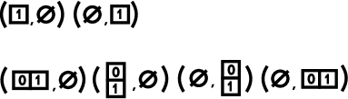
Fig. 2: Samples of Young diagrams contributing in the case of $SU(2)$ and $r=2$. The upper corresponds to $k_{0}=0$ of case 1 and the lower corresponds to $k_{0}=1$ of case 2. The number drawn in each box is the respective $\mathbb{Z}_{r}$-charge.

Let us consider

$$Z^{(2)}_{k_{0}+1/2}:=\lim_{h\to 0}\frac{h^{2}}{2^{2}}\sum_{|A|+|B|=2k_{0}+1}\widetilde{\mathcal{A}}_{AB}^{(1,1)},$$ (5.30)

$$Z^{(2)}_{k_{0}}:=\lim_{h\to 0}\sum_{|A|+|B|=2k_{0}}\widetilde{\mathcal{A}}_{AB}^{(0,0)}.$$ (5.31)

Here $\mathcal{A}_{AB}^{(x,y)}$ represents that two Young diagrams $A$ and $B$ have the $\mathbb{Z}_{2}$-charge $x$ and $y$ respectively. The coefficient $h^{2}/2^{2}$ in the definition of $Z^{(2)}_{k_{0}+1/2}$ has introduced in order to remove the coefficients in (5.21) and (5.25). From (5.31) and (5.30), we will now check that the $\mathbb{R}^{4}/\mathbb{Z}_{2}$ partition function is

$$Z^{\mathbb{R}^{4}/\mathbb{Z}_{2}}_{SU(2)}=\sum_{k_{0}=0}^{\infty}\left({\Lambda^{\prime}}\right)^{k_{0}}Z^{(2)}_{k_{0}}+\sum_{k_{0}=0}^{\infty}\left({\Lambda}^{\prime}\right)^{k_{0}+1/2}Z^{(2)}_{k_{0}+1/2},$$ (5.32)

by the explicit calculation. First of all, in the case $k_{0}=0~{}(k=1)$ of case 1, expanding around $h=0$, we have

$$\widetilde{\mathcal{A}}_{(1)(0)}^{(1,1)}=\frac{2^{2}}{h^{2}}\left(\frac{-1}{2a(2a-\epsilon_{1}-\epsilon_{2})}+O(h)\right),~{}~{}\widetilde{\mathcal{A}}_{(0)(1)}^{(1,1)}=\frac{2^{2}}{h^{2}}\left(\frac{-1}{2a(2a+\epsilon_{1}+\epsilon_{2})}+O(h)\right).$$ (5.33)

Therefore,

$$Z^{(2)}_{1/2}=\lim_{h\to 0}\frac{h^{2}}{2^{2}}(\widetilde{\mathcal{A}}_{(1)(0)}^{(1,1)}+\widetilde{\mathcal{A}}_{(0)(1)}^{(1,1)})=-\frac{2}{(2a+\epsilon_{1}+\epsilon_{2})(2a-\epsilon_{1}-\epsilon_{2})}.$$ (5.34)

Next, in the case $k_{0}=1~{}(k=2)$ of case 2,

$$\begin{split}\widetilde{\mathcal{A}}_{(2),(0)}&=\frac{\prod_{i=1}^{2}[m_{i}+a]_{q}[-(m_{i+2}+a)]_{q}[m_{i}+a+1]_{q}[-(m_{i+2}+a+1)]_{q}}{[1+\beta]_{q}[-2]_{q}[\beta]_{q}[-1]_{q}[-2a-1+\beta]_{q}[2a]_{q}[-2a-2+\beta]_{q}[2a+1]_{q}},\\ \widetilde{\mathcal{A}}_{(1,1),(0)}&=\frac{\prod_{i=1}^{2}[m_{i}+a]_{q}[-(m_{i+2}+a)]_{q}[m_{i}+a-\beta]_{q}[-(m_{i+2}+a-\beta)]_{q}}{[2\beta]_{q}[-1-\beta]_{q}[\beta]_{q}[-1]_{q}[-2a+2\beta-1]_{q}[2a-\beta]_{q}[-2a-1+\beta]_{q}[2a]_{q}},\\ \widetilde{\mathcal{A}}_{(1),(1)}&=\frac{\prod_{i=1}^{2}[m_{i}+a]_{q}[-(m_{i+2}+a)]_{q}[m_{i}-a]_{q}[-(m_{i+2}-a)]_{q}}{[\beta]_{q}[-1]_{q}[\beta]_{q}[-1]_{q}[-2a+\beta]_{q}[2a-1]_{q}[2a+\beta]_{q}[-2a-1]_{q}},\\ \widetilde{\mathcal{A}}_{(0),(1,1)}&=\frac{\prod_{i=1}^{2}[m_{i}-a]_{q}[-(m_{i+2}-a)]_{q}[m_{i}-a-\beta]_{q}[-(m_{i+2}-a-\beta)]_{q}}{[2\beta]_{q}[-1-\beta]_{q}[\beta]_{q}[-1]_{q}[2a+2\beta-1]_{q}[-2a-\beta]_{q}[2a-1+\beta]_{q}[-2a]_{q}},\\ \widetilde{\mathcal{A}}_{(0),(2)}&=\frac{\prod_{i=1}^{2}[m_{i}-a]_{q}[-(m_{i+2}-a)]_{q}[m_{i}-a+1]_{q}[-(m_{i+2}-a+1)]_{q}}{[1+\beta]_{q}[-2]_{q}[\beta]_{q}[-1]_{q}[2a-1+\beta]_{q}[-2a]_{q}[2a-2+\beta]_{q}[-2a+1]_{q}}.\end{split}$$ (5.35)

Assigning the charge (0,0), we obtain

$$\begin{split}\widetilde{\mathcal{A}}_{(2)(0)}^{(0,0)}&=\frac{\prod_{i=1}^{4}(m_{i}+a)}{(-2\epsilon_{2})(\epsilon_{1}-\epsilon_{2})(2a+\epsilon_{1}+\epsilon_{2})2a}+O(h),\\ \widetilde{\mathcal{A}}_{(1,1)(0)}^{(0,0)}&=\frac{\prod_{i=1}^{4}(m_{i}+a)}{2\epsilon_{1}(\epsilon_{1}-\epsilon_{2})(2a+\epsilon_{1}+\epsilon_{2})2a}+O(h),\\ \widetilde{\mathcal{A}}_{(1)(1)}^{(0,0)}&=\frac{h^{8}}{2^{8}}\prod_{i=1}^{4}(m_{i}+a)(m_{i}-a)+O(h^{9}),\\ \widetilde{\mathcal{A}}_{(0)(1,1)}^{(0,0)}&=\frac{\prod_{i=1}^{4}(m_{i}-a)}{2\epsilon_{1}(\epsilon_{1}-\epsilon_{2})(2a-\epsilon_{1}-\epsilon_{2}))2a}+O(h),\\ \widetilde{\mathcal{A}}_{(0)(2)}^{(0,0)}&=\frac{\prod_{i=1}^{4}(m_{i}-a)}{(-2\epsilon_{2})(\epsilon_{1}-\epsilon_{2})(2a-\epsilon_{1}-\epsilon_{2})2a}+O(h).\end{split}$$ (5.36)

and

$$Z^{(2)}_{1} =\lim_{h\to 0}\left(\widetilde{\mathcal{A}}_{(2)(0)}^{(0,0)}+\widetilde{\mathcal{A}}_{(1,1)(0)}^{(0,0)}+\widetilde{\mathcal{A}}_{(1)(1)}^{(0,0)}+\widetilde{\mathcal{A}}_{(0)(1,1)}^{(0,0)}+\widetilde{\mathcal{A}}_{(0)(2)}^{(0,0)}\right)$$ (5.37)

$$=-\frac{\prod_{i=1}^{4}(m_{i}+a)}{\epsilon_{1}\epsilon_{2}(2a+\epsilon_{1}+\epsilon_{2})4a}-\frac{\prod_{i=1}^{4}(m_{i}-a)}{\epsilon_{1}\epsilon_{2}(2a-\epsilon_{1}-\epsilon_{2})4a}.$$ (5.38)

Note that $\widetilde{\mathcal{A}}_{(1)(1)}^{(0,0)}$ which does not satisfy (5.8) becomes automatically 0 in this limiting procedure.

Similarly, in the case $k=3$ and $k=4$ we obtain the following results,

$$Z^{(2)}_{3/2} \scriptstyle{=\underset{h\to 0}{\lim}\frac{h^{2}}{2^{2}}(\widetilde{\mathcal{A}}_{(3)(0)}^{(1,1)}+\widetilde{\mathcal{A}}_{(2,1)(0)}^{(1,1)}+\widetilde{\mathcal{A}}_{(1,1,1)(0)}^{(1,1)}+\widetilde{\mathcal{A}}_{(2)(1)}^{(1,1)}+\widetilde{\mathcal{A}}_{(1,1)(1)}^{(1,1)}+\widetilde{\mathcal{A}}_{(0)(3)}^{(1,1)}+\widetilde{\mathcal{A}}_{(0)(2,1)}^{(1,1)}+\widetilde{\mathcal{A}}_{(0)(1,1,1)}^{(1,1)}+\widetilde{\mathcal{A}}_{(1)(2)}^{(1,1)}+\widetilde{\mathcal{A}}_{(1)(1,1)}^{(1,1)})}$$ (5.39)

$$\scriptstyle{=\frac{\prod_{i=1}^{4}(m_{i}+a+\epsilon_{2})}{(-\epsilon_{1}+\epsilon_{2})(-2\epsilon_{2})(-2a-\epsilon_{1}-\epsilon_{2})(2a)(-2a-\epsilon_{1}-3\epsilon_{2})(2a+2\epsilon_{2})}+\frac{\prod_{i=1}^{4}(m_{i}+a+\epsilon_{1})}{(-2\epsilon_{1})(\epsilon_{1}-\epsilon_{2})(-2a-3\epsilon_{1}-\epsilon_{2})(2a+2\epsilon_{1})(-2a-\epsilon_{1}-\epsilon_{2})(2a)}}$$ (5.40)

$$~{}~{}\scriptstyle{+\frac{\prod_{i=1}^{4}(m_{i}+a+\epsilon_{2})}{(-\epsilon_{1}+\epsilon_{2})(-2\epsilon_{2})(-2a-\epsilon_{1}-\epsilon_{2})(2a)(2a-\epsilon_{1}+\epsilon_{2})(-2a-2\epsilon_{2})}}\scriptstyle{+\frac{\prod_{i=1}^{4}(m_{i}+a+\epsilon_{1})}{(-2\epsilon_{1})(\epsilon_{1}-\epsilon_{2})(-2a-2\epsilon_{1})(2a+\epsilon_{1}-\epsilon_{2})(-2a-\epsilon_{1}-\epsilon_{2})(2a)}}$$ (5.41)

$$~{}~{}\scriptstyle{+\frac{\prod_{i=1}^{4}(m_{i}-a+\epsilon_{2})}{(-\epsilon_{1}+\epsilon_{2})(-2\epsilon_{2})(2a-\epsilon_{1}-\epsilon_{2})(2a)(2a-3\epsilon_{2}-\epsilon_{1})(-2a+2\epsilon_{2})}+\frac{\prod_{i=1}^{4}(m_{i}-a+\epsilon_{1})}{(-2\epsilon_{1})(\epsilon_{1}-\epsilon_{2})(2a-3\epsilon_{1}-\epsilon_{2})(-2a+2\epsilon_{1})(2a-\epsilon_{1}-\epsilon_{2})(-2a)}}$$ (5.42)

$$~{}~{}\scriptstyle{+\frac{\prod_{i=1}^{4}(m_{i}-a+\epsilon_{2})}{(-\epsilon_{1}+\epsilon_{2})(-2\epsilon_{2})(2a-\epsilon_{1}-\epsilon_{2})(-2a)(-2a-\epsilon_{1}+\epsilon_{2})(2a-2\epsilon_{2})}}\scriptstyle{+\frac{\prod_{i=1}^{4}(m_{i}-a+\epsilon_{1})}{(-2\epsilon_{1})(\epsilon_{1}-\epsilon_{2})(2a-2\epsilon_{1})(-2a+\epsilon_{1}-\epsilon_{2})(2a-\epsilon_{1}-\epsilon_{2})(-2a)}},$$ (5.43)

and

$$Z^{(2)}_{2} =\scriptstyle{\frac{\prod_{i=1}^{4}(m_{i}+a)(m_{i}+a+2\epsilon_{2})}{(-\epsilon_{1}+3\epsilon_{2})(-4\epsilon_{2})(-\epsilon_{1}+\epsilon_{2})(-2\epsilon_{2})(-2a-\epsilon_{1}-\epsilon_{2})(2a)(-2a-\epsilon_{1}-3\epsilon_{2})(2a+2\epsilon_{2})}}$$ (5.44)

$$~{}~{}~{}\scriptstyle{+\frac{\prod_{i=1}^{4}(m_{i}+a)(m_{i}+a+2\epsilon_{2})}{(-\epsilon_{1}+\epsilon_{2})(\epsilon_{1}-3\epsilon_{2})(-\epsilon_{1}+\epsilon_{2})(-2\epsilon_{2})(-2a-\epsilon_{1}-3\epsilon_{2})(2a+2\epsilon_{2})(-2a-\epsilon_{1}-\epsilon_{2})(2a)}}$$ (5.45)

$$~{}~{}~{}\scriptstyle{+\frac{\prod_{i=1}^{4}(m_{i}+a)(m_{i}+a+\epsilon_{1}+\epsilon_{2})}{(-2\epsilon_{1})(\epsilon_{1}-\epsilon_{2})(-\epsilon_{1}+\epsilon_{2})(-2\epsilon_{2})(-2a-2\epsilon_{1}-2\epsilon_{2})(2a+\epsilon_{1}+\epsilon_{2})(-2a-\epsilon_{1}-\epsilon_{2})(2a)}}$$ (5.46)

$$~{}~{}~{}\scriptstyle{+\frac{\prod_{i=1}^{4}(m_{i}+a)(m_{i}+a+2\epsilon_{1})}{(-3\epsilon_{1}+\epsilon_{2})(2\epsilon_{1}-2\epsilon_{2})(-2\epsilon_{1})(\epsilon_{1}-\epsilon_{2})(-2a-3\epsilon_{1}-\epsilon_{2})(2a+2\epsilon_{1})(-2a-\epsilon_{1}-\epsilon_{2})(2a)}}$$ (5.47)

$$~{}~{}~{}\scriptstyle{+\frac{\prod_{i=1}^{4}(m_{i}+a)(m_{i}+a+2\epsilon_{1})}{(-4\epsilon_{1})(3\epsilon_{1}-\epsilon_{2})(-2\epsilon_{1})(\epsilon_{1}-\epsilon_{2})(-2a-3\epsilon_{1}-\epsilon_{2})(2a+2\epsilon_{1})(-2a-\epsilon_{1}-\epsilon_{2})(2a)}}$$ (5.48)

$$~{}~{}~{}\scriptstyle{+\frac{\prod_{i=1}^{4}(m_{i}+a)(m_{i}-a)}{(-2a-2\epsilon_{1})(2a+\epsilon_{1}-\epsilon_{2})(-2a-\epsilon_{1}-\epsilon_{2})(2a)(-2a-\epsilon_{1}-\epsilon_{2})(2a)(2a-\epsilon_{1}+\epsilon_{2})(-2a-2\epsilon_{2})}}$$ (5.49)

$$~{}~{}~{}\scriptstyle{+\frac{\prod_{i=1}^{4}(m_{i}+a)(m_{i}-a)}{(-\epsilon_{1}+\epsilon_{2})(-2\epsilon_{2})(-2\epsilon_{1})(\epsilon_{1}-\epsilon_{2})(-2a-\epsilon_{1}-\epsilon_{2})(2a)(2a-\epsilon_{1}-\epsilon_{2})(-2a)}}$$ (5.50)

$$~{}~{}~{}\scriptstyle{+\frac{\prod_{i=1}^{4}(m_{i}+a)(m_{i}-a)}{(\epsilon_{2}-\epsilon_{1})^{2}(-2\epsilon_{2})^{2}(-2a-\epsilon_{1}+\epsilon_{2})(2a-2\epsilon_{2})(2a-\epsilon_{1}+\epsilon_{2})(-2a-2\epsilon_{2})}}$$ (5.51)

$$~{}~{}~{}\scriptstyle{+\frac{\prod_{i=1}^{4}(m_{i}+a)(m_{i}-a)}{(\epsilon_{1}-\epsilon_{2})^{2}(-2\epsilon_{1})^{2}(-2a+\epsilon_{1}-\epsilon_{2})(2a-2\epsilon_{1})(2a+\epsilon_{1}-\epsilon_{2})(-2a-2\epsilon_{1})}}$$ (5.52)

$$~{}~{}~{}\scriptstyle{+\frac{\prod_{i=1}^{4}(m_{i}+a)(m_{i}+a+2\epsilon_{2})}{(-\epsilon_{1}+3\epsilon_{2})(-4\epsilon_{2})(-\epsilon_{1}+\epsilon_{2})(-2\epsilon_{2})(2a-\epsilon_{1}-\epsilon_{2})(-2a)(2a-\epsilon_{1}-3\epsilon_{2})(-2a+2\epsilon_{2})}}$$ (5.53)

$$~{}~{}~{}\scriptstyle{+\frac{\prod_{i=1}^{4}(m_{i}+a)(m_{i}+a+2\epsilon_{2})}{(-\epsilon_{1}+\epsilon_{2})(\epsilon_{1}-3\epsilon_{2})(-\epsilon_{1}+\epsilon_{2})(-2\epsilon_{2})(2a-\epsilon_{1}-3\epsilon_{2})(-2a+2\epsilon_{2})(2a-\epsilon_{1}-\epsilon_{2})(-2a)}}$$ (5.54)

$$~{}~{}~{}\scriptstyle{+\frac{\prod_{i=1}^{4}(m_{i}+a)(m_{i}+a+\epsilon_{1}+\epsilon_{2})}{(-2\epsilon_{1})(\epsilon_{1}-\epsilon_{2})(-\epsilon_{1}+\epsilon_{2})(-2\epsilon_{2})(2a-2\epsilon_{1}-2\epsilon_{2})(-2a+\epsilon_{1}+\epsilon_{2})(2a-\epsilon_{1}-\epsilon_{2})(-2a)}}$$ (5.55)

$$~{}~{}~{}\scriptstyle{+\frac{\prod_{i=1}^{4}(m_{i}+a)(m_{i}+a+2\epsilon_{1})}{(-3\epsilon_{1}+\epsilon_{2})(2\epsilon_{1}-2\epsilon_{2})(-2\epsilon_{1})(\epsilon_{1}-\epsilon_{2})(2a-3\epsilon_{1}-\epsilon_{2})(-2a+2\epsilon_{1})(2a-\epsilon_{1}-\epsilon_{2})(-2a)}}$$ (5.56)

$$~{}~{}~{}\scriptstyle{+\frac{\prod_{i=1}^{4}(m_{i}+a)(m_{i}+a+2\epsilon_{1})}{(-4\epsilon_{1})(3\epsilon_{1}-\epsilon_{2})(-2\epsilon_{1})(\epsilon_{1}-\epsilon_{2})(2a-3\epsilon_{1}-\epsilon_{2})(-2a+2\epsilon_{1})(2a-\epsilon_{1}-\epsilon_{2})(-2a)}}$$ (5.57)

$$~{}~{}~{}\scriptstyle{+\frac{\prod_{i=1}^{4}(m_{i}+a)(m_{i}-a)}{(2a-2\epsilon_{1})(-2a+\epsilon_{1}-\epsilon_{2})(2a-\epsilon_{1}-\epsilon_{2})(-2a)(2a-\epsilon_{1}-\epsilon_{2})(-2a)(-2a-\epsilon_{1}+\epsilon_{2})(2a-2\epsilon_{2})}}$$ (5.58)

$$~{}~{}~{}\scriptstyle{+\frac{\prod_{i=1}^{4}(m_{i}+a)(m_{i}-a)}{(-\epsilon_{1}+\epsilon_{2})(-2\epsilon_{2})(-2\epsilon_{1})(\epsilon_{1}-\epsilon_{2})(2a-\epsilon_{1}-\epsilon_{2})(-2a)(-2a-\epsilon_{1}-\epsilon_{2})(2a)}}.$$ (5.59)

If we consider the limit in which the fundamental matters decouple, the pure Yang-Mills case is reproduced. [29]

In the case of general $r$, setting $k_{\ell}=k_{0}+\delta k_{\ell}$,  ${\ell}=0,\cdots,r-1$, we find from the condition (5.8),

$$q_{a}=0~{}~{}~{}\delta k_{\ell}=(0,\cdots,0),$$ (5.60)

$$q_{a}\neq 0~{}~{}~{}\delta k_{\ell}=(0,1,2,\cdots,\underset{{\ell}=q_{a}}{q_{a}},\cdots,\underset{{\ell}=r-q_{a}}{q_{a}},q_{a}-1,\cdots,1).$$ (5.61)

Here

$$0\leq q_{a}\leq r-q_{a}~{}~{}~{}~{}~{}\Rightarrow~{}~{}~{}~{}~{}0\leq q_{a}\leq\left\lfloor\frac{r}{2}\right\rfloor.$$ (5.62)

The total number of boxes in the case of $\mathbb{Z}_{r}$ charge $q_{a}$ is $rk_{0}+q_{a}(r-q_{a})$. Therefore, we define

$$Z^{(r)}_{k_{0}+\frac{q_{a}(r-q_{a})}{r}}:=\lim_{h\to 0}\Xi_{q_{a}}\sum_{\begin{subarray}{c}|A|+|B|\\ =rk_{0}+q_{a}(r-q_{a})\end{subarray}}\widetilde{\mathcal{A}}_{AB}^{(q_{a},-q_{a})}.$$ (5.63)

Now if we assume that $\Xi_{q_{a}}$ does not depend on $k$ and is equal to each other for all $\widetilde{\mathcal{A}}_{AB}$ involved we are able to evaluate this quantity for a typical Young diagram. At least, we can see that this assumption is correct at the lower levels of $SU(2)$, $r=2$. One of the case $k_{0}=0$ is drawn in Fig. 3. After the computation on this diagram, we find that we should set

$$\Xi_{0}=1,~{}~{}~{}~{}\Xi_{1}=h^{2}\frac{1}{(1-\omega)(1-\omega^{-1})},$$ (5.64)

$$\Xi_{q_{a}}=h^{2q_{a}}\frac{\prod_{i=1}^{q_{a}-1}(1-\omega^{i})^{2q_{a}-3i}(1-\omega^{-i})^{2q_{a}-3i}}{\prod_{j=1}^{q_{a}}(1-\omega^{q_{a}+j-1})^{q_{a}-j+1}(1-\omega^{-(q_{a}+j-1)})^{q_{a}-j+1}},~{}~{}~{}~{}~{}~{}~{}~{}~{}2\leq q_{a}\leq\left\lfloor\frac{r}{2}\right\rfloor.$$ (5.65)

Then $\mathbb{R}^{4}/\mathbb{Z}_{r}$ instanton partition function is

$$Z^{\mathbb{R}^{4}/\mathbb{Z}_{r}}_{SU(2)}=\sum_{q_{a}=0}^{\lfloor\frac{r}{2}\rfloor}\sum_{k_{0}=0}^{\infty}\left({\Lambda^{\prime}}\right)^{k_{0}+\frac{q_{a}(r-q_{a})}{r}}Z^{(r)}_{k_{0}+\frac{q_{a}(r-q_{a})}{r}}.$$ (5.66)

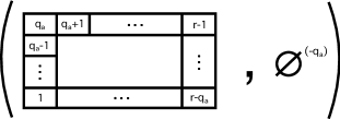
Fig. 3: Example of $n$-tuple Young diagram in the case of $k_{0}=0$, $SU(2)$ and general $r$.

In the case of $SU(n)$ and general $r$, we can start with (5.10). From the condition (5.8), we find

$$\delta k_{\ell}=\biggl{(}0,(n-1),\cdots,\underset{{\ell}=q_{n-1}}{q_{n-1}(n-1)},q_{n-1}(n-1)+(n-2),\cdots,\underset{{\ell}=q_{n-2}}{q_{n-1}+q_{n-2}(n-2)},$$ (5.67)

$$~{}~{}~{}~{}~{}\cdots,\underset{{\ell}=q_{n-(j-1)}}{\sum_{i=1}^{j-2}q_{n-i}+q_{n-j+1}(n-j+1)},\sum_{i=1}^{j-2}q_{n-i}+q_{n-j+1}(n-j+1)+(n-j),$$ (5.68)

$$~{}~{}~{}~{}~{}\cdots,\underset{{\ell}=q_{n-j}}{\sum_{i=1}^{j-1}q_{n-i}+(n-j)q_{n-j}},\cdots,\underset{{\ell}=q_{1}}{\sum_{i=1}^{n-1}q_{n-i}},\cdots,\underset{{\ell}=r-\sum_{i=1}^{n-1}q_{i}}{\sum_{i=1}^{n-1}q_{n-i}},\sum_{i=1}^{n-1}q_{n-i}-1,\cdots,1\biggl{)}.$$ (5.69)

Here we have set

$$r-\sum_{i=1}^{n-1}q_{i}\geq q_{1}\geq q_{2}\geq\cdots\geq q_{n-1}\geq 0~{}~{}~{}({\rm mod}~{}r),$$ (5.70)

All other cases on these inequalities can be obtained by the appropriate interchange of the numbers $q_{1},\cdots,q_{n-1}$. So we do not lose any generality. The total number of boxes is $k_{0}r+d$. Here

$$d=\sum_{\alpha=1}^{n-1}{q_{\alpha}}\left(r-\sum_{\alpha^{\prime}=1}^{\alpha}q_{\alpha^{\prime}}\right).$$ (5.71)

Let us define

$$Z^{(r)}_{k_{0}+\frac{d}{r}}:=\lim_{h\to 0}\Xi_{q_{\alpha}}\sum_{\begin{subarray}{c}|\vec{Y}|\\ =rk_{0}+d\end{subarray}}\widetilde{\mathcal{A}}_{\vec{Y}}^{(q_{\alpha})}.$$ (5.72)

Here $(q_{\alpha})=(q_{1},\cdots,q_{n-1},q_{n}),~{}q_{n}=-q_{1}-\cdots-q_{n-1}$ is $\mathbb{Z}_{r}$-charge assigned to each Young diagram in $\vec{Y}$. Computing the case of Fig. 4, we obtain the coefficient

$$\Xi_{q_{\alpha}}=h^{2\sum_{\alpha=1}^{n-1}\alpha q_{\alpha}}\xi_{q_{\alpha}}(\omega)\xi_{q_{\alpha}}(\omega^{-1}),$$ (5.73)

$$\xi_{q_{\alpha}}(\omega)= \prod_{a<b}^{n-1}\prod_{j=1}^{q_{b}-1}\frac{(1-\omega^{j})^{2(q_{b}-j)}}{(1-\omega^{\sum_{i=a}^{b-1}q_{i}+j})^{q_{b}-j}(1-\omega^{\sum_{i=a}^{b-1}q_{i}+j})^{q_{b}-j}}\frac{1}{(1-\omega^{\sum_{i=a}^{b-1}q_{i}})^{q_{b}}}$$ (5.74)

$$\times\prod_{a=1}^{n-1}\prod_{j=1}^{q_{a}-1}\frac{(1-\omega^{j})^{q_{a}-j}(1-\omega^{\sum_{i=a+1}^{n-1}q_{i}+j})^{q_{a}-j}}{(1-\omega^{\sum_{i=1}^{a-1}q_{i}+j})^{j}(1-\omega^{\sum_{i=1}^{n-1}q_{i}+j})^{q_{a}-j}}\frac{1}{(1-\omega^{\sum_{i=1}^{a}q_{i}})^{q_{a}}}$$ (5.75)

$$\times\prod_{a=1}^{n-1}\prod_{j=1}^{q_{a+1}+\cdots q_{n-1}}\frac{(1-\omega^{j})^{q_{a}}}{(1-\omega^{\sum_{i=1}^{a}q_{i}+j})^{q_{a}}}$$ (5.76)

$$\times\prod_{a+2\leq b}^{n-1}\prod_{j=1}^{q_{b}-1}\frac{(1-\omega^{j})^{j}(1-\omega^{\sum_{i=a+1}^{b-1}q_{i}+j})^{q_{b}-j}}{(1-\omega^{q_{a}-q_{b}+j})^{j}(1-\omega^{\sum_{i=k}^{l-1}q_{i}-j})^{j}}\prod_{j=0}^{q_{a+1}+\cdots+q_{b-1}-q_{b}}\frac{(1-\omega^{q_{b}+j})^{q_{b}}}{(1-\omega^{q_{a}+j})^{q_{b}}}.$$ (5.77)

Then the $\mathbb{R}^{4}/\mathbb{Z}_{r}$ instanton partition function is given by

$$Z^{\mathbb{R}^{4}/\mathbb{Z}_{r}}_{SU(n)}=\sum_{q_{\alpha}}\sum_{k=0}^{\infty}(\Lambda^{\prime})^{k+\frac{d}{r}}Z^{(r)}_{k+\frac{d}{r}}.$$ (5.78)

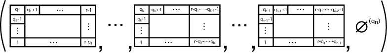
Fig. 4: Example of $n$-tuple Young diagram in the case of $k_{0}=0$, $SU(n)$ and $r$. The total number of boxes is equal to $d$.

To summarize, the method of obtaining the $SU(n)$ instanton partition function on $\mathbb{R}^{4}/\mathbb{Z}_{r}$ from the five dimensional instanton partition function by the limiting procedure (5.16) has been established. The ALE instanton partition functions are systematically obtained by using (5.72)-(5.78).

6 Note added

References we became aware after submission include [66, 67, 68].

References

- [1] A. A. Belavin, A. M. Polyakov, and A. B. Zamolodchikov, “Infinite conformal symmetry in two-dimensional quantum field theory,” Nucl. Phys. B 241, 333-380 (1984).
- [2] H. Nakajima, Lectures on Hilbert Schemes of points on surfaces, American Mathematical Society (1999).
- [3] N. Nekrasov, “Seiberg-Witten prepotential from instanton counting,” Adv. Theor. Math. Phys. 7, 831-864 (2004) [arXiv:hep-th/0206161].
- [4] L. F. Alday, D. Gaiotto, and Y. Tachikawa, “Liouville Correlation Functions from Four-dimensional Gauge Theories,” Lett. Math. Phys. 9, 167-197 (2010) [arXiv:0906.3219 [hep-th]].
- [5] N. Wyllard, “ conformal Toda field theory correlation functions from conformal quiver gauge theories,” JHEP 0911, 002 (2009) [arXiv:0907.2189 [hep-th]].
- [6] R. Dijkgraaf and C. Vafa, “Toda Theories, Matrix Models, Topological Strings, and Gauge Systems,” arXiv:0909.2453 [hep-th].
- [7] H. Itoyama, K. Maruyoshi and T. Oota, “The Quiver Matrix Model and 2d-4d Conformal Connection,” Prog. Theor. Phys. 123, 957-987 (2010) [arXiv:0911.4244 [hep-th]].
- [8] A. Mironov, A. Morozov and Sh. Shakirov, “Matrix Model Conjecture for Exact BS Periods and Nekrasov Functions,” JHEP 1002, 030 (2010) [arXiv:0911.5721 [hep-th]].
- [9] A. Mironov, A. Morozov and Sh. Shakirov, “Conformal blocks as Dotsenko-Fateev Integral Discriminants,” J. Mod. Phys. A 25, 3173-3207 (2010) [arXiv:1001.0563 [hep-th]].
- [10] H. Itoyama and T. Oota, “Method of generating -expansion coefficients for conformal block and Nekrasov function by -deformed matrix model,” Nucl. Phys. B 838, 298-330 (2010) [arXiv:1003.2929 [hep-th]].
- [11] A. Mironov, A. Morozov and And. Morozov, “Matrix model version of AGT conjecture and generalized Selberg integrals,” Nucl. Phys. B 843, 534-557 (2011) [arXiv:1003.5752 [hep-th]].
- [12] H. Itoyama, T. Oota and N. Yonezawa, “Massive scaling limit of the -deformed matrix model of Selberg type,” Phys. Rev. D 82, 085031 (2010) [arXiv:1008.1861 [hep-th]].
- [13] T. Nishinaka and C. Rim, “-Deformed Matrix Model and Nekrasov Partition Function,” JHEP 1202, 114 (2012) [arXiv:1112.3545 [hep-th]].
- [14] F. Fucito, J. F. Morales and D. R. Pacifici, “Deformed Seiberg-Witten curves for ADE quivers,” JHEP 1301, 091 (2013) [arXiv:1210.3580 [hep-th]].
- [15] J. Kaneko, “-Selberg integrals and Macdonald polynomials,” Ann. scient. Éc. Norm. Sup. 29, 583-637 (1996).
- [16] K. W. J. Kadell, “The Selberg-Jack Symmetric Functions,” Adv. Math. 130, 33-102 (1997).
- [17] V. A. Fateev and A. V. Litvinov, “On AGT conjecture,” JHEP 1002, 014 (2010) [arXiv:0912.0504 [hep-th]].
- [18] M. Hadasz, Z. Jaskólski and P. Suchanek, “Proving the AGT relation for antifundamentals,” JHEP 1006, 046 (2010) [arXiv:arXiv:1004.1841 [hep-th]].
- [19] A. Mironov, A. Morozov and Sh. Shakirov, “A direct proof of AGT conjecture at ,” JHEP 1102, 067 (2011) [arXiv:1012.3137 [hep-th]].
- [20] A. Morozov and A. Smirnov, “Finalizing the proof of AGT relations with the help of the generalized Jack polynomial”, arXiv:1307.2576 [hep-th].
- [21] Workshops for JSPS/RFBR bilateral collaboration project “Progress in the synthesis of integrabilities arising from gauge-string duality”, Viale Osaka, Osaka, Japan, March 23-25, 2013 and Center for Cultural Exchange, Osaka City University, Osaka, Japan, June 5, 2013; International Conference on Integrable Systems and Quantum symmetries, Prague, Czech Republic, June 12-16, 2013.
- [22] J. Shiraishi, H. Kubo, H. Awata and S. Odake, “A quantum deformation of the Virasoro algebra and the Macdonald symmetric functions,” Lett. Math. Phys. 38, 33-51 (1996) [arXiv:q-alg/9507034].
- [23] E. Frenkel and N. Reshetikhin, “Towards deformed chiral algebras,” in Quantum Group Symposium at Group 21: Proceedings of the Quantum Group Symposium at the XXI International Colloquium on Group Theoretical Methods on Physics (Goslar, 1996), eds. by H.-D. Doebner and V. K. Dobrev, Academica Press (1997), pp. 27-42 [arXiv:q-alg/9706023].
- [24] H. Awata, H. Kubo, S. Odake and J. Shiraishi, “Quantum Algebras and Macdonald Polynomials,” Commun. Math. Phys. 179, 401-416 (1996) [arXiv:q-alg/9508011].
- [25] H. Awata, H. Kubo, Y. Morita, S. Odake and J. Shiraishi, “Vertex Operators of the -Virasoro Algebra; Defining Relations, Adjoint Actions and Four Point Functions,” Lett. Math. Phys. 41, 65-78 (1997) [arXiv:q-alg/9604023].
- [26] H. Awata and Y. Yamada, “Five-dimensional AGT Conjecture and the Deformed Virasoro algebra,” JHEP 1001, 125 (2010) [arXiv:0910.4431 [hep-th]; “Five-Dimensional AGT Relation and the Deformed -Ensemble,” Prog. Theor. Phys. 124, 227-262 (2010) [arXiv:1004.5122 [hep-th]].
- [27] P. Bouwknegt and K. Pilch, “The Deformed Virasoro Algebra at Roots of Unity,” Commun. Math. Phys. 196, 249-288 (1998) [arXiv:q-alg/9710026].
- [28] V. Belavin and B. Feigin, “Super Liouville conformal blocks from quiver gauge theories,” JHEP 1107, 079 (2011) [arXiv:1105.5800 [hep-th]].
- [29] G. Bonelli, K. Maruyoshi and A. Tanzini, “Instantons on ALE spaces and super Liouville conformal field theories,” JHEP 1108, 056 (2011) [arXiv:1106.2505 [hep-th]]; “Gauge Theories on ALE Space and Super Liouville Correlation Functions,” Lett. Math. Phys. 101, 103-124 (2012) [arXiv:1107.4609 [hep-th]].
- [30] A. Belavin, V. Belavin and M. Bershtein, “Instantons and 2d Superconformal field theory,” JHEP 1109, 117 (2011) [arXiv:1106.4001 [hep-th]].
- [31] N. Wyllard, “Coset conformal blocks and gauge theories,” arXiv:1109.4264 [hep-th].
- [32] M. N. Alfimov and G. M. Tarnopolsky, “Parafermionic Liouville field theory and instantons on ALE spaces,” JHEP 1202, 036 (2012) [arXiv:1110.5628 [hep-th]].
- [33] Y. Ito, “Ramond sector of super Liouville theory from instantons on an ALE space,” Nucl. Phys. B 861, 387-402 (2012) [arXiv:1110.2176 [hep-th]].
- [34] A. A. Belavin, M. A. Bershtein, B. L. Feigin, A. V. Litvinov and G. M. Tarnopolsky, “Instanton moduli spaces and bases in coset conformal field theory,” Commun. Math. Phys. 319, 269-301 (2013) [arXiv:1111.2803 [hep-th]].
- [35] A. A. Belavin, M. A. Bershtein and G. M. Tarnopolsky, “Bases in coset conformal field theory from AGT correspondence and Macdonald polynomials at the roots of unity,” arXiv:1211.2788 [hep-th].
- [36] M. N. Alfimov, A. A. Belavin and G. M. Tarnopolsky, “Coset conformal field theory and instanton counting on ,” arXiv:1306.3938 [hep-th].
- [37] V. A. Belavin, “ SUSY Conformal Block Recursive Relations,” hep-th/0611295.
- [38] D. Friedan, Z. Qiu and S. H. Shenker, “Superconformal invariance in two dimensions and the tricritical Ising model,” Phys. Lett. B 151, 37-43 (1985).
- [39] H. Eichenherr, “Minimal operator algebras in superconformal quantum field theory,” Phys. Lett. B 151, 26-30 (1985).
- [40] M. A. Bershadsky, V. G. Knizhnik and M. G. Teitelman, “Superconformal symmetry in two dimensions,” Phys. Lett. B 151, 31-36 (1985).
- [41] S. O. Warnaar, “-Selberg integrals and Macdonald polynomials,” Ramanujan J. 10, 237-268 (2005).
- [42] P. J. Forrester and S. O. Warnaar, “ The Importance of the Selberg Integral,” Bull. Amer. Math. Soc. 45, 489-534 (2008) [arXiv:0710.3981 [math.CA]].
- [43] S. O. Warnaar, “A Selberg integral for the Lie algebra ,” Acta Math. 203, 269-304 (2009) [arXiv:0708.1193 [math.CA]].
- [44] H. Nakajima, “Instantons on ALE spaces, quiver varieties, and Kac-Moody algebras,” Duke Math. J. 76, 365-416 (1994).
- [45] H. Nakajima, “Quiver varieties and Kac-Moody algebras,” Duke Math. J. 91, 515-560 (1998).
- [46] H. Nakajima, “Jack polynomials and Hilbert schemes of points on surfaces,” arXiv:alg-geom/9610021.
- [47] H. Nakajima, “Heisenberg algebra and Hilbert schemes of points on projective surfaces,” Ann. Math. 145, 379-388 (1997) [arXiv:alg-geom/9507012].
- [48] H. Nakajima, “Quiver varieties and finite dimensional representations of quantum affine algebras,” J. Am. Math. Soc, 14, 145-238 (2001) [arXiv:math/9912158 [math.QA]].
- [49] H. Nakajima and K. Yoshioka, “Instanton counting on blowup. I. 4-dimensional pure gauge theory,” J. Invent. Math. 162, 313-355 (2005) [arXiv:math/0306198 [math.AG]].
- [50] P. Kronheimer and H. Nakajima, “Yang-Mills instantons on ALE gravitational instantons,” Math. Ann. 288, 263-307 (1990).
- [51] H. Awata and H. Kanno, “Refined BPS state counting from Nekrasov’s formula and Macdonald functions,” Int. J. Mod. Phys. A 24, 2253-2306 (2009) [arXiv:0805.0191 [hep-th]].
- [52] M. -C. Tan, “M-theoretic derivations of 4d-2d dualities: from a geometric Langlands duality for surfaces, to the AGT Correspondence, to integrable systems,” JHEP 1307, 171 (2013) [arXiv:1301.1977 [hep-th]].
- [53] F. Nieri, S. Pasquetti and F. Passerini,“3d & 5d gauge theory partition functions as -deformed CFT correlators,” arXiv:1303.2626 [hep-th].
- [54] J. Lepowsky and R. L. Wilson, “Construction of the Affine Lie Algebra ,” Commun. math. Phys. 62, 43-53 (1978).
- [55] Y. Kitazawa, N. Ishibashi, A. Kato, K. Kobayashi, Y. Matsuo and S. Odake, “Operator product expansion coefficients in superconformal theory and slightly relevant perturbation,” Nucl. Phys. B 306, 425-444 (1988).
- [56] L. Alvarez-Gaumé and Ph. Zaugg, “Structure constants in the superoperator algebra,” Annals Phys. 215, 171-230 (1992) [hep-th/9109050].
- [57] A. B. Zamolodchikov and V. A. Fateev, “Nonlocal (parafermion) currents in two-dimensional conformal quantum field theory and self-dual critical points in -symmetric statistical systems,” Sov. Phys. JETP 62, 215-225 (1985) [Zh. Eksp. Teor. Fiz. 89, 380-399 (1985)].
- [58] D. Gepner and Z. Qiu, “Modular invariant partition functions for parafermionic field theories,” Nucl. Phys. B 285, 423-453 (1987).
- [59] M. A. Bershtein, V. A. Fateev and A. V. Litvinov, “Parafermionic polynomials, Selberg integrals and three-point correlation function in parafermionic Liouville field theory,” Nucl. Phys. B 847, 413-459 (2011) [arXiv:1011.4090 [hep-th]].
- [60] B. Feigin and E. Frenkel, “Quantum -Algebras and Elliptic Algebras,” Commun. Math. Phys. 178, 653-678 (1996) [arXiv:q-alg/9508011].
- [61] V. S. Dotsenko and V. A. Fateev, “Conformal algebra and multipoint correlation functions in 2D statistical models,” Nucl. Phys. B 240, 312-348 (1984).
- [62] H. Zhang and Y. Matsuo, “Selberg Integral and AGT Conjecture,” JHEP 1112, 106 (2011) [arXiv:1110.5255 [hep-th]].
- [63] A. Mironov, A. Morozov, Sh. Shakirov and A. Smirnov, “Proving AGT conjecture as HS duality: Extension to five dimensions,” Nucl. Phys. B 855, 128-151 (2012) [arXiv:1105.0948 [hep-th]].
- [64] F. Fucito, J. F. Morales and R. Poghossian, “Multi-instanton calculus on ALE spaces,” Nucl. Phys. B 703, 518-536 (2004) [arXiv:hep-th/0406243].
- [65] T. Kimura, “Matrix model from orbifold partition function,” JHEP 1109, 015 (2011) [arXiv:1105.6091 [hep-th]].
- [66] B. Estienne, V. Pasquier, R. Santachiara and D. Serban, “Conformal blocks in Virasoro and W theories: Duality and the Calogero-Sutherland model,” Nucl. Phys. B 860, 377-420 (2012) [arXiv:1110.1101 [hep-th]].
- [67] V. Pasquier and D. Serban, “Conformal field theory and edge excitations for the principal series of quantum Hall fluids,” Phys. Rev. B 63, 153311 (2001) [arXiv:cond-mat/9912218].
- [68] G. Cristofano, G. Maiella and V. Marotta, “A twisted conformal field theory description of the quantum Hall effect,” Mod. Phys. Lett. A15, 547-555 (2000) [arXiv:cond-mat/9912287].