Longtime behavior of coupled wave equations for semiconductor lasers

Abstract

Coupled wave equations are popular tool for investigating longitudinal dynamical effects in semiconductor lasers, for example, sensitivity to delayed optical feedback. We study a model that consists of a hyperbolic linear system of partial differential equations with one spatial dimension, which is nonlinearly coupled with a slow subsystem of ordinary differential equations. We first prove the basic statements about the existence of solutions of the initial-boundary-value problem and their smooth dependence on initial values and parameters. Hence, the model constitutes a smooth infinite-dimensional dynamical system. Then we exploit the particular slow-fast structure of the system to construct a low-dimensional attracting invariant manifold for certain parameter constellations. The flow on this invariant manifold is described by a system of ordinary differential equations that is accessible to classical bifurcation theory and numerical tools such as AUTO.

1 Introduction

Semiconductor lasers are known to be extremely sensitive to delayed optical feedback. Even small amounts of feedback may destabilize the laser and cause a variety of nonlinear effects. Self-pulsations, excitability, coexistence of several stable regimes, and chaotic behavior have been observed both in experiments and in numerical simulations (see [1, 2] for general reviews). Due to their inherent speed, semiconductor lasers are of great interest for modern optical data transmission and telecommunication technology if these nonlinear feedback effects can be cultivated and controlled. Potential applications include, for example, clock recovery [3], generation of pulse trains [4] or high-frequency oscillations [5], and pulse reshaping [6].

Typically, these applications utilize the laser in a non-stationary mode, for example, to produce high-frequency oscillations or pulse trains. Multi-section DFB (distributed feedback) lasers allow one to engineer these nonlinear effects by designing the longitudinal structure of the device [7]. If mathematical modeling is to be helpful in guiding this difficult and expensive design process it has to use models that are, on one hand, as accurate as possible and, on the other hand, give insight into the nature of the observed nonlinear phenomena. The latter is only possible by a detailed bifurcation analysis, while only models involving partial differential equations (PDEs) describe the effects with the necessary accuracy.

We focus in this paper on coupled wave equations with gain dispersion. This model is a system of PDEs (one-dimensional in space), which are nonlinearly coupled to ordinary differential equations (ODEs). It is accurate enough to show quantitatively good correspondence with experiments and more detailed models [5, 6]. We prove in this paper that the model can be reduced to a low-dimensional system of ODEs analytically. This makes the model accessible to well-established and powerful numerical bifurcation analysis tools such as Auto [8]. This in turn allows us to construct detailed and accurate numerical bifurcation diagrams for many practically relevant situations; see [6, 9] for recent results and section 7 for an illustrative example.

We achieve the central goal of our paper, the proof of the model reduction, in three steps. First, we show that the PDE system establishing the coupled wave model is a smooth infinite-dimensional dynamical system, that is, it generates a semiflow that is strongly continuous in time and smooth with respect to initial values and parameters. Then, we exploit the particular structure of the model which is of the form

$$\begin{split}\dot{E}&=\ H(n)E\\ \dot{n}&=\varepsilon f(n,E)\end{split}$$ (1)

where the light amplitude $E\in\mathbb{L}^{2}([0,L];\mathbb{C}^{4})$ is infinite-dimensional and the effective carrier density $n\in\mathbb{R}^{m}$ is finite-dimensional. The small parameter $\varepsilon$ expresses that the carrier density $n$ operates on a much slower time-scale than $E$. Hence, we investigate in the second step the growth properties of the semigroup generated by $H$ for fixed $n$, proving the existence of spectral gaps. In the last step we construct a low-dimensional invariant manifold for small $\varepsilon$ using the general theory on the persistence and properties of normally hyperbolic invariant manifolds for strongly continuous semiflows in Banach spaces [10, 11, 12].

The paper is organized as follows. In Section 2, we introduce the coupled wave model as described in [13] and explain the physical meaning of all variables and parameters. Section 3 summarizes the results of the paper in a non-technical but precise fashion. It points out the difficulties and the methods and theory used in the proofs. In Section 4 we formulate the PDE system as an abstract evolution equation in a Hilbert space and prove that it establishes a smooth infinite-dimensional system in this setting. In this section, we consider also inhomogeneous boundary conditions in (1) modeling optical injection into the laser. In Section 5 we investigate the spectral properties of the operator $H$ for fixed $n$ and homogeneous boundary conditions and find $n$ such that $H(n)$ has a spectral gap to the left of the imaginary axis. Section 6 is concerned with the construction of a finite-dimensional attracting invariant manifold, where we make use of the slow-fast structure of (1) and the results of Section 4 and Section 5.

Finally, in Section 7 we explain how the system of ODEs obtained in Section 6 can be made accessible to standard numerical bifurcation analysis tools like AUTO. We present an illustrative and relevant example to demonstrate the usefulness of the model reduction. Moreover, we extend the model reduction theorem of Section 6 to delay differential equations (DDEs), which are widely used to study delayed feedback effects in lasers [1].

2 Coupled wave equations with gain dispersion

The coupled wave model, a hyperbolic system of PDEs coupled with a system of ODEs is a well known model describing the longitudinal effects in classical semiconductor lasers [13, 16]. It has been derived from Maxwell’s equations for an electro-magnetic field in a periodically modulated waveguide [13] assuming that transversal and longitudinal effects can be separated. In this section we introduce the corresponding system of differential equations, explain the physical interpretation of its coefficients and specify all physically sensible assumptions about these coefficients.

The variable $\psi(t,z)\in\mathbb{C}^{2}$ describes the complex amplitude of the slowly varying envelope of the optical field split into a forward and a backward traveling wave. The variable $p(t,z)\in\mathbb{C}^{2}$ describes the corresponding nonlinear polarization of the material. Both quantities depend on time and the one-dimensional spatial variable $z\in[0,L]$ (the longitudinal direction within the laser). A prominent feature of multi-section lasers is the splitting of the overall interval $[0,L]$ into sections, that is, $m$ subintervals $S_{k}$ that represent sections with separate electric contacts. The other dependent variable $n(t)\in\mathbb{R}^{m}$ describes the section-wise spatially averaged carrier density within each section $S_{k}$. In dimensionless form the initial-boundary value problem for $\psi$, $p$, and $n$ reads as (dropping the arguments $t$ and $z$; all coefficients are discussed below):

$$\partial_{t}\psi =\begin{bmatrix}-1&0\\[-4.30554pt] \phantom{-}0&1\end{bmatrix}\partial_{z}\psi-\begin{bmatrix}0&i\\[-4.30554pt] i&0\end{bmatrix}\kappa\,\psi+\bigl{[}(1+i\alpha_{H})\,G(n)-d\bigr{]}\,\psi+\rho(n)\,\bigl{[}p-\psi\bigr{]}$$ (2)

$$\partial_{t}p =[i\Omega_{r}(n)-\Gamma(n)]\,p+\Gamma(n)\,\psi$$ (3)

and for $$k=1\ldots m$$

$$\dot{n}_{k} =I_{k}-\frac{n_{k}}{\tau_{k}}-\frac{P}{l_{k}}\int\limits_{z_{k}}^{z_{k+1}}\left[\begin{array}[c]{cc}\psi\\ p\end{array}\right]^{*}\left[\begin{array}[c]{ccc}G_{k}(n_{k})-\rho_{k}(n_{k})&&\frac{1}{2}\rho_{k}(n_{k})\\ \frac{1}{2}\rho_{k}(n_{k})&&0\end{array}\right]\left[\begin{array}[c]{c}\psi\\ p\end{array}\right]\mbox{d}z$$ (10)

$$=:f_{k}(n_{k},(\psi,p))\mbox{.}$$

System (2)–(10) is subject to the inhomogeneous boundary conditions for $\psi$

$$\psi_{1}(t,0)=r_{0}\psi_{2}(t,0)+\alpha(t)\mbox{,\ }\psi_{2}(t,L)=r_{L}\psi_{1}(t,L)$$ (11)

and the initial conditions

$$\psi(0,z)=\psi^{0}(z)\mbox{,\ }p(0,z)=p^{0}(z)\mbox{,\ }n(0)=n^{0}\mbox{.}$$ (12)

The Hermitian transpose of a $\mathbb{C}^{4}$ vector is denoted by $[\cdot]^{*}$ in (10). The length of the laser is $L$. We denote the length of subinterval $S_{k}$ by $l_{k}$ and its starting point by $z_{k}$ (for $k=1\ldots m$). We scale $z$ such that $l_{1}=z_{2}=1$ and denote $z_{m+1}=L$. Thus, $S_{k}=[z_{k},z_{k+1}]$. All coefficients of (2), (3) are spatially constant in each subinterval $S_{k}$ and depend only on $n_{k}$, that is, if $z\in S_{k}$,

$$\kappa(z) =\ \kappa_{k}\in\mathbb{R}\mbox{,\quad} d(z) =d_{k}\in\mathbb{C}\mbox{,\quad} \alpha_{H}(z) =\alpha_{H,k}\in\mathbb{R}\mbox{,}$$ (12)

$$G(n,z) =G_{k}(n_{k})\in\mathbb{R}\mbox{,\quad} \rho(n,z) =\rho_{k}(n_{k})\in\mathbb{R}\mbox{,\quad} \Omega_{r}(n,z) =\Omega_{r,k}(n_{k})\in\mathbb{R}\mbox{,}$$ (12)

$$\Gamma(n,z) =\ \Gamma_{k}(n_{k})\in\mathbb{R}\mbox{.}$$ (12)

The permissible range of $n_{k}$ is the interval $(\underline{n},\infty)$ where, typically, $\underline{n}=-\infty$ or $\underline{n}=0$. We assume that the functions $\rho$, $\Omega$, and $\Gamma$ are Lipschitz continuous, and smooth in $(\underline{n},\infty)$. Moreover, $\Omega$ and $\Gamma$ are bounded globally. The function $G_{k}:(\underline{n},\infty)\to\mathbb{R}$ is a smooth strictly monotone increasing function satisfying $G_{k}(1)=0$, $G_{k}^{\prime}(1)>0$, $\lim_{\nu\searrow\underline{n}}G_{k}(\nu)=-\infty$, and $\lim_{\nu\to\infty}G_{k}(\nu)=\infty$. Typical models for $G_{k}$ are

$$G_{k}(\nu) =\ \tilde{g}_{k}\log\nu \mbox{(}\underline{n} =\ 0\mbox{) or}$$ (13)

$$G_{k}(\nu) =\ \tilde{g}_{k}\cdot(\nu-1) \mbox{(}\underline{n} =\ -\infty\mbox{)}$$

where $\tilde{g}_{k}=G_{k}^{\prime}(1)>0$. Physically sensible assumptions on the parameters throughout the paper are $\operatorname{Re}d_{k}>0$, $\Gamma_{k}(n_{k})>1$, $0<I_{k}\ll 1$, $\tau_{k}\gg 1$. Furthermore, $\rho_{k}(n_{k})$ is bounded for $n_{k}\searrow\underline{n}$, $\rho_{k}(n_{k})\geq 0$ for $n_{k}\geq 1$ and $\rho_{k}(n_{k})/G_{k}(n_{k})\to 0$ for $n_{k}\to\infty$. In (11) $r_{0}$ and $r_{L}\in\mathbb{C}$ satisfy $|r_{0}|<1$ and $|r_{L}|<1$. All other coefficients (as well as their Lipschitz constants if they depend on $n$) are of order $1$. The constant $P$ determines the scaling of $(\psi,p)$. It can be chosen arbitrarily. We denote the right-hand-side of the carrier density equation (10) for $n_{k}$ by $f_{k}(n_{k},(\psi,p))$ observing that $f_{k}$ is Hermitian in $(\psi,p)$. Collecting $\psi$ and $p$ into one $\mathbb{C}^{4}$ vector $E=(\psi,p)^{T}$ system (2)–(10) assumes the form of (1) discussed in the introduction. In particular, Equations (2), (3) are linear in $\psi$ and $p$ if the inhomogeneity $\alpha(t)$ equals zero.

Physical background and motivation of the model

Equation (2) describes the transport of the two complex profiles $\psi_{1}$ (forward) and $\psi_{2}$ (backward) in a waveguide from $z=0$ to $z=L$. The boundary conditions (11) describe the reflection at the facettes at $z=0$ and $z=L$ of the laser with complex reflectivities of modulus less than $1$ and, possibly, a complex optical input $\alpha(t)$. The case of discontiuous optical input $\alpha(t)$ is of interest in applications (for example, square-wave signals, or noisy signals).

The number of sections, $m$, is typically small. For example, the prototype device studied in [6, 9] has $m=2$. The coupling between the wave profiles $\psi_{1}$ and $\psi_{2}$, expressed by a non-zero $\kappa$ in (2), is achieved by a small-scale spatial modulation of the refractive index of the waveguide. Equation (2) considers only the spatially averaged coupling effect, called distributed feedback, which affords the name DFB laser.

The function $G_{k}$, called gain, expresses the dependence of the amplification of $\psi$ (stimulated emission of photons) on the carrier density $n_{k}$ in each section. The gain $G_{k}(n_{k})$ is positive if $n_{k}>1$ and negative if $n_{k}<1$. The real part of $d_{k}$ is positive expressing the waveguide losses. A nonzero coefficient $\alpha_{H,k}$ (called the Henry factor, typically $\alpha_{k,H}\in(0,10)$) expresses the fact that an increase of the carrier density $n_{k}$ not only increases the amplification in the waveguide but also changes its refractive index. This effect is regarded as one of the main reasons behind the extreme sensitivity of semiconductor lasers with respect to optical feedback [2].

Taking into account the polarization $p$ introduces the effect of gain dispersion, which means that the light amplification depends on the frequency of the light, prefering frequencies close to $\Omega_{r}$. This effect is rather weak in long semiconductor lasers (which means $\Gamma\gg 1$) but it breaks the symmetry $[\lambda+\operatorname{Re}d-G(n),E(z)]\to[G(n)-\operatorname{Re}d-\bar{\lambda},\bar{E}(L-z)]$ of the eigenvalue problem $\lambda E=H(n)E$ corresponding to the fast subsystem in (1) in the case of a single section ($m=1$). This symmetry breaking has a significant effect on the observed dynamics also in the multi-section case [13]. In combination with the non-zero coupling $\kappa$ the presence of a positive $\rho_{k}(n_{k})$ for at least one section $S_{k}$ and a finite $\Gamma_{k}(n_{k})$ guarantee the existence of a spectral gap for the linear operator $H(n)$ in (1), which will be needed for the construction of the invariant manifold.

The dynamics of the carrier density ((10) in section $S_{k}$) is governed by three terms: the constant current input $I_{k}$, a decay with rate $\tau_{k}^{-1}$, and the stimulated recombination, spatially averaged over $S_{k}$. The stimulated recombination is Hermitian in $E=(\psi,p)^{T}$. The coefficients $G_{k}(n_{k})$ and $\rho_{k}(n_{k})$ are such that the $n_{k}$-dependent matrix in the integrand is positive definite for $n_{k}\to\infty$ and negative definite for $n_{k}\searrow\underline{n}$. The smallness of the parameters $I_{k}$ and $\tau_{k}^{-1}$ in the appropriate non-dimensionalization and the choice of a small $P$ makes $\dot{n}_{k}$ small. That is, $n$ is a slow variable compared to $E=(\psi,p)^{T}$ [1].

3 Non-technical overview

In this section we state the main results of the paper in a non-technical but precise manner and summarize the methods used in the proofs of these results. We have split this section into four parts. First we show that system (2)–(10) generates a smooth infinite-dimensional dynamical system. Then we introduce a small parameter. In the next step we investigate the dynamics of the (linear) infinite-dimensional fast subsystem, and finally we construct a low-dimensional attracting invariant manifold.

3.1 Existence theory

In a first step we investigate in which sense system (2)–(10) generates a semiflow depending smoothly on its initial values and all parameters; for details see section 4. Our aim is to write (2)–(10) as an abstract evolution equation in the form

$$\frac{d}{dt}u=Au+g(u)$$

in a Hilbert space $V$ where $A$ is a linear differential operator that generates a strongly continuous semigroup $S(t)$ and $g$ is smooth in $V$. A natural space for the variables $\psi$ and $p$ is $\mathbb{L}^{2}([0,L];\mathbb{C}^{2})$, such that $V$ could be $\mathbb{L}^{2}([0,L];\mathbb{C}^{2})\times\mathbb{L}^{2}([0,L];\mathbb{C}^{2})\times\mathbb{R}^{m}$ for the variable $u=(\psi,p,n)$. However, the inhomogeneity $\alpha$ in the boundary condition (11) does not fit into this framework. Common approaches such as boundary homogenization (used in [3]) require a high degree of regularity of $\alpha$ in time, which is unnatural as the laser still works with discontinuous input. To avoid the introduction of the concept of weakly mild solutions (as was done in [17]), we introduce the auxiliary space-dependent variable $a(t,x)$ ($x\in[0,\infty)$) satisfying the equation

$$\partial_{t}a(t,x)=\partial_{x}a(t,x)$$ (14)

and change the boundary condition for $z=0$ in (11) into $\psi_{1}(t,0)=r_{0}\psi_{2}(t,0)+a(t,0)\mbox{.}$ One may think of an infinitely long fibre $[0,\infty)$ storing all future optical inputs and transporting them to the laser facet $z=x=0$ by the transport equation (14). If we choose $a(0,x)=\alpha(x)$ as initial value for $a$ then the value of $a$ at the boundary $x=0$ at time $t$ is $\alpha(t)$. In this way, the formerly inhomogeneous boundary condition becomes linear in the variables $\psi$ and $a$ requiring no regularity for $a$. To keep the space $V$ a Hilbert space, we choose a weighted $\mathbb{L}^{2}$ norm for $a$ that contains $\mathbb{L}^{\infty}$, that is, $\|a(t,\cdot)\|^{2}=\int_{0}^{\infty}|a(t,x)|^{2}(1+x^{2})^{\eta}\,dx$ with $\eta<-1/2$.

With this modification we can work within the framework of the theory of strongly continuous semigroups [18]. The variable $u$ has the components $(\psi,p,n,a)\in V=\mathbb{L}^{2}([0,L];\mathbb{C}^{2})\times\mathbb{L}^{2}([0,L];\mathbb{C}^{2})\times\mathbb{R}^{m}\times\mathbb{L}^{2}_{\eta}([0,\infty);\mathbb{C})$. We have a certain freedom how to choose the splitting of the right-hand-side between $A$ and $g$. We keep $A$ as simple as possible, including only the unbounded terms

$$A\,\left[(\psi,p,n,a)^{\,T}\right]:=\left([-\partial_{z}\psi,\partial_{z}\psi],0,0,\partial_{x}a\right)^{\,T}\mbox{.}$$

In this way, it is easy to prove that $A$ generates a strongly continuous semigroup $S(t)$ by constructing $S$ explicitly. The nonlinearity $g$ is smooth because it is a superposition operator of smooth coefficient functions, and all components either depend only linearly on the infinite-dimensional components $\psi$ and $p$, or map into $\mathbb{R}^{m}$. Then, the existence of a semiflow $S(t;u)$ that is strongly continuous in $t$ and smooth with respect to $u$ and parameters follows from an a-priori estimate. This a-priori estimate is more subtle than the one in [3]. It uses the fact that there is dissipation (for $\operatorname{Re}d_{k}>0$) and that the same functions $G_{k}$ and $\rho_{k}$ appear on the right-hand-side of (2) and of (10) but with opposing signs. Due to this fact we can show that the function

$$\frac{P}{2}\|\psi(t)\|^{2}+\sum_{k=1}^{m}l_{k}(n_{k}(t)-n_{*})$$

remains non-negative for sufficiently small $n_{*}$ and, hence, bounded, giving rise to a bounded invariant ball in $V$.

3.2 Introduction of a small parameter

For all results about the long-time behavior of system (2)–(10) we restrict ourselves to autonomous boundary conditions for $\psi$, that is,

$$\psi_{1}(t,0)=r_{0}\psi_{2}(t,0)\mbox{,\quad}\psi_{2}(t,L)=r_{L}\psi_{1}(t,L)\mbox{.}$$ (15)

The inhomogeneous case is an open question for future work. However, understanding the dynamics of the autonomous laser is not only an intermediate step but an important goal in itself since many experiments and simulations focus on this case; see, for example, [5] for further references.

We exploit that $I_{k}$ and $\tau_{k}^{-1}$ in (10) are approximately two orders of magnitude smaller than $1$ by introducing a small parameter $\varepsilon$. We set $P=\varepsilon$ in (10) such that the set of carrier density equations (10) reads as

$$\frac{d}{dt}n=f\left(n,E\right)=\varepsilon F(n,E)$$ (16)

where all coefficients of $F=f/\varepsilon$ are of order $1$ in all $m$ components of $F$, and $E=(\psi,p)^{T}$. The space dependent subsystem (2), (3) is linear in $E$

$$\frac{d}{dt}E=H(n)E$$ (17)

where $H(n)$ has the form

$$H(n)=\begin{bmatrix}\begin{bmatrix}-\partial_{z}+\beta(n)&-i\kappa\\ -i\kappa&\partial_{z}+\beta(n)\end{bmatrix}&\rho(n)\\[10.00002pt] \Gamma(n)&i\Omega_{r}(n)-\Gamma(n)\end{bmatrix}$$ (18)

and $\beta(n)=(1+i\alpha_{H})G(n)-d-\rho(n)$. For fixed $n$, $H(n)$ acts from

$$Y:=\{(\psi,p)\in\mathbb{H}^{1}([0,L];\mathbb{C}^{2})\times\mathbb{L}^{2}([0,L];\mathbb{C}^{2}):\\ \psi_{1}(0)=r_{0}\psi_{2}(0)\mbox{,\ }\psi_{2}(L)=r_{L}\psi_{1}(L)\}$$

into $X=\mathbb{L}^{2}([0,L];\mathbb{C}^{2})\times\mathbb{L}^{2}([0,L];\mathbb{C}^{2})$. The operator $H(n)$ generates a $C_{0}$ semigroup $T(n;t):X\to X$. The coefficients $\kappa$, and, for each $n\in(\underline{n},\infty)^{m}$, $\beta(n)$, $\Omega_{r}(n)$, $\Gamma(n)$ and $\rho(n)$ are linear operators in $\mathbb{L}^{2}([0,L];\mathbb{C}^{2})$ defined by the corresponding coefficients in (2), (3). The maps $\beta$, $\rho$, $\Gamma$, and $\Omega_{r}:\mathbb{R}^{m}\to\mathcal{L}(\mathbb{L}^{2}([0,L];\mathbb{C}^{2}))$ are smooth.

Although $\varepsilon$ is not directly accessible, we treat it as a parameter and consider the limit $\varepsilon\to 0$ while keeping $F$ fixed. At $\varepsilon=0$, the carrier density $n$ is constant. It enters the linear subsystem (17) as a parameter. Thus, the spectral properties of $H(n)$ determine the long-time behavior of system (16), (17) for $\varepsilon=0$. Section 3.4 (and Section 6 in detail) will study in which sense this fact can be exploited to find exponentially attracting invariant manifolds also for small $\varepsilon$.

3.3 Spectral properties of $H(n)$

The goal of Section 5 is to show that there exist carrier densities $n$ such that $H(n)$ (and, correspondingly, $T(n;t)$) has a spectral gap. More precisely, we investigate if there exists a $n\in(\underline{n},\infty)^{m}$, and a splitting of $X=X_{c}(n)\oplus X_{s}(n)$ into two $H(n)$-invariant subspaces such that $X_{c}(n)$ is finite-dimensional, the spectrum of $H(n)|_{X_{c}(n)}$ is on the imaginary axis, and the semigroup $T(n;\cdot)|_{X_{s}(n)}$ satisfies

$$\|T(n;t)|_{X_{s}}\|\leq Me^{-\xi t}$$ (19)

for some $\xi>0$ and $M\geq 1$ and all $t\geq 0$. Carrier densities $n$ for which $H(n)$ has this splitting are called critical. Generically they form submanifolds (with boundary) of $\mathbb{R}^{m}$ of dimension $m-q$ where $q=\dim_{\mathbb{C}}X_{c}(n)$.

The strongly continuous semigroup $T(n;t)$ is a compact perturbation of the semigroup $T_{0}(n;t)$ generated by the diagonal part $H_{0}(n)$ of $H(n)$ [19]. The essential spectral radius $\exp(tR_{\infty}(n))$ of $T_{0}$ can be found analytically. To prove the existence of a critical carrier density $n$ with spectral gap we have to find a $n\in(\underline{n},\infty)^{m}$ such that $R_{\infty}(n)<0$ but the characteristic function $h(n;\cdot)$ of $H(n)$ (which is known analytically) has roots on the imaginary axis. This is possible if one of the following two conditions is satisfied

1. The coupling $\kappa_{k}$ is nonzero for at least one $k\in\{1,\ldots,m\}$, and $m\geq 2$.

2. The reflectivities satisfy $r_{0}r_{L}\neq 0$, and $\rho_{k}(\nu)>0$ for all $\nu>1$ for at least one $k\in\{1,\ldots,m\}$.

These two conditions state precisely in which sense the coupling $\kappa_{k}$ and the gain dispersion $\rho_{k}(n)$ guarantee the spectral gap of $H(n)$ (as mentioned already in Section 2).

3.4 Existence of a low-dimensional invariant manifold

Let $\mathcal{K}\subset\mathbb{R}^{m}$ be a manifold of critical carrier densities with uniform spectral gap. The dimension of the critical subspace $X_{c}(n)$ is constant, say, $q\geq 1$. For $\varepsilon=0$ and a sufficiently small neighborhood $U$ of $\mathcal{K}$ the set

$$\mathcal{C}_{0}:=\{(E,n):n\in U,E\in X_{c}(n),\|E\|\leq R\}$$

is invariant and exponentially attracting in its $E$-component. Theorem 7 in Section 6, the main nonlinear result, proves that this invariant manifold persists also for small $\varepsilon>0$. For $k\geq 2$, and sufficiently small $\varepsilon>0$ and $U\supset\mathcal{K}$, system (16),(17) has a $C^{k}$ manifold $\mathcal{C}$ that is invariant and exponentially attracting relative to $\{(E,n):\|E\|\leq R,n\in U\}$. It can be described as a $C^{1}$-small graph over $\mathcal{C}_{0}$. The semiflow restricted to $\mathcal{C}$ is governed by the ODE in $\mathbb{C}^{q}\times\mathbb{R}^{m}$

$$\begin{split}\frac{d}{dt}E_{c}&=\ \left[H_{c}(n)+\varepsilon a_{1}(E_{c},n,\varepsilon)+\varepsilon^{2}a_{2}(E_{c},n,\varepsilon)\nu(E_{c},n,\varepsilon)\right]E_{c}\\ \frac{d}{dt}n_{\phantom{k}}&=\ \varepsilon F(n,[B(n)+\varepsilon\nu(E_{c},n,\varepsilon)]E_{c})\end{split}$$ (20)

where $H_{c}(n)=H(n)|_{X_{c}(n)}$, $B(n)$ is a basis of $X_{c}(n)$, $\nu\in C^{k-2}$, and

$$\begin{split}a_{1}(E_{c},n,\varepsilon)&=\ -B(n)^{-1}P_{c}(n)\partial_{n}B(n)F(n,[B(n)+\varepsilon\nu(E_{c},n,\varepsilon)]E_{c})\\ a_{2}(E_{c},n,\varepsilon)&=\ B(n)^{-1}\partial_{n}P_{c}(n)F(n,[B(n)+\varepsilon\nu(E_{c},n,\varepsilon)]E_{c})[I-P_{c}(n)]\end{split}$$

where $P_{c}(n)$ is the spectral projection onto $X_{c}(n)$ for $H(n)$.

Theorem 7 is an application of the general theory about persistence of normally hyperbolic invariant manifolds of semiflows under $C^{1}$ small perturbations [10, 11, 12]. The unperturbed invariant manifold $\mathcal{C}_{0}$ is finite-dimensional and exponentially stable. The proof describes in detail the appropriate cut-off modification of the system outside of the region of interest to make the unperturbed invariant manifold compact. Then it connects the results of the previous sections to guarantee the $C^{1}$-smallness of the perturbation and the normal hyperbolicity of $\mathcal{C}_{0}$. A similar model reduction result has been proven in [22] for ODEs of the structure (1) using Fenichel’s Theorem for singularly perturbed systems of ODEs [23]. Since Fenichel’s Theorem is not available for infinite-dimensional systems, we have to adapt the proof in [23] to our case starting from the general results in [10, 11, 12] about invariant manifolds of semiflows in Banach spaces. In particular, we apply the cut-off modifications done in [23] only to the finite-dimensional components $E_{c}$ and $n$. Moreover, we adapt the modifications such that the invariant manifold for $\varepsilon=0$ is compact without boundary as required by the theorems in [10].

4 Existence of a smooth semiflow

In this section, we treat the inhomogeneous initial-boundary value problem (2)-(11) as an autonomous nonlinear evolution equation

$$\frac{d}{dt}u(t)=Au(t)+g(u(t))\mbox{,\hskip 10.00002pt}u(0)=u_{0}$$ (21)

where $u(t)$ is an element of a Hilbert space $V$, $A$ is a generator of a $C_{0}$ semigroup $S(t)$, and $g:U\subseteq V\to V$ is smooth and locally Lipschitz continuous in an open set $U\subseteq V$. The inhomogeneity in (11) is included in (21) as a component of $u$.

The Hilbert space $V$ is defined by

$$V:=\mathbb{L}^{2}([0,L];\mathbb{C}^{2})\times\mathbb{L}^{2}([0,L];\mathbb{C}^{2})\times\mathbb{R}^{m}\times\mathbb{L}^{2}_{\eta}([0,\infty);\mathbb{C})$$ (22)

where $\mathbb{L}^{2}_{\eta}([0,\infty);\mathbb{C})$ is the space of weighted square integrable functions. The scalar product of $\mathbb{L}^{2}_{\eta}([0,\infty);\mathbb{C})$ is defined by

$$(v,w)_{\eta}:=\operatorname{Re}\int_{0}^{\infty}\bar{v}(x)\cdot w(x)(1+x^{2})^{\eta}dx\mbox{.}$$

We choose $\eta<-1/2$ such that the space $\mathbb{L}^{\infty}([0,\infty);\mathbb{C})$ is continuously embedded in $\mathbb{L}^{2}_{\eta}([0,\infty);\mathbb{C})$. The complex plane is treated as two-dimensional real plane in the definition of the vector space $V$ such that the standard $\mathbb{L}^{2}$ scalar product $(\cdot,\cdot)_{V}$ of $V$ is differentiable. The corresponding components of a vector $v\in V$ are denoted by

$$v=(\psi,p,n,a).$$

Here, $\psi$ and $p$ have two complex components and $n\in\mathbb{R}^{m}$. The spatial variable in $\psi$ and $p$ is denoted by $z\in[0,L]$, whereas the spatial variable in $a$ is denoted by $x\in[0,\infty)$. The Hilbert space $\mathbb{H}^{1}_{\eta}([0,\infty);\mathbb{C})$ equipped with the scalar product

$$(v,w)_{1,\eta}:=(v,w)_{\eta}+(\partial_{x}v,\partial_{x}w)_{\eta}$$

is densely and continuously embedded in $\mathbb{L}^{2}_{\eta}([0,\infty);\mathbb{C})$. Moreover, its elements are continuous [25]. Consequently, the Hilbert spaces

$$W := \mathbb{H}^{1}([0,L];\mathbb{C}^{2})\times\mathbb{L}^{2}([0,L];\mathbb{C}^{2})\times\mathbb{R}^{m}\times\mathbb{H}^{1}_{\eta}([0,\infty);\mathbb{C})\mbox{,\ and}$$

$$W_{\mathrm{BC}} := \{(\psi,p,n,a)\in W:\psi_{1}(0)=r_{0}\psi_{2}(0)+a(0),\psi_{2}(L)=r_{L}\psi_{1}(L)\}$$

are densely and continuously embedded in $V$. The linear functionals $\psi_{1}(0)-r_{0}\psi_{2}(0)-a(0)$ and $\psi_{2}(L)-r_{L}\psi_{1}(L)$ are continuous from $W\to\mathbb{R}$. We define the linear operator $A:W_{\mathrm{BC}}\to V$ by

$$A\begin{bmatrix}\psi\\[-4.30554pt] p\\[-4.30554pt] n\\[-4.30554pt] a\end{bmatrix}:=\begin{bmatrix}\begin{bmatrix}-\partial_{z}&0\\[-4.30554pt] \phantom{-}0&\partial_{z}\end{bmatrix}\,\psi\\[-4.30554pt] 0\\[-4.30554pt] 0\\[-4.30554pt] \partial_{x}a\end{bmatrix}\mbox{.}$$ (23)

The definition of $A$ and $W_{\mathrm{BC}}$ treat the inhomogeneity $\alpha$ in the boundary condition (11) as the boundary value of the variable $a$ at $0$. We define the open set $U\subseteq V$ by

$$U:=\{(\psi,p,n,a)\in V:n_{k}>\underline{n}\mbox{\ for\ }k=1\ldots m\}\mbox{,}$$

and the nonlinear function $g:U\to V$ by

$$g(\psi,p,n,a)=\begin{pmatrix}\left[(1+i\alpha_{H})G(n)-d\right]\psi-i\kappa\begin{bmatrix}0&1\\[-6.45831pt] 1&0\end{bmatrix}\psi+\rho(n)[p-\psi]\\[10.00002pt] (i\Omega_{r}(n)-\Gamma(n))p+\Gamma(n)\psi\\[5.0pt] \left(f_{k}(n_{k},(\psi,p))\right)_{k=1}^{m}\\ 0\end{pmatrix}\mbox{.}$$ (24)

The corresponding coefficients of (2)–(10) define the smooth maps $G,\rho,\Omega_{r},\Gamma:(\underline{n},\infty)^{m}\to\mathcal{L}(\mathbb{L}^{2}([0,L];\mathbb{C}^{2}))$. The function $g$ is continuously differentiable to any order with respect to all arguments and its Frechet derivative is bounded in any closed bounded ball $B\subset U$. Thus, (21) with the right-hand-side defined by (23), (24) fits into the framework of the theory of $C_{0}$ semigroups [18].

The inhomogeneous initial-boundary value problem (2)-(12) and the autonomous evolution system (21) are equivalent in the following sense: Suppose $\alpha\in\mathbb{H}^{1}([0,T);\mathbb{C})$ in (11). Let $u=(\psi,p,n,a)$ be a classical solution of (21), satisfying (21) in the $\mathbb{L}^{2}$ sense. Then $u$ satisfies (2)-(3), and (12) in $\mathbb{L}^{2}$ and (10), (11) for each $t\in[0,T]$ if and only if $a^{0}|_{[0,T]}=\alpha$. On the other hand, assume that $(\psi,p,n)$ satisfies (2)-(3), and (12) in $\mathbb{L}^{2}$ and (10), (11) for each $t\in[0,T]$. Then, choosing $a^{0}\in\mathbb{H}^{1}_{\eta}([0,\infty);\mathbb{C})$ such that $a^{0}|_{[0,T]}=\alpha$, we obtain that $u(t)=(\psi(t),p(t),n(t),a^{0}(t+\cdot))$ is a classical solution of (21) in $[0,T]$.

We prove in Lemma 1 that $A$ generates a $C_{0}$ semigroup $S(t)$ in $V$. Mild solutions of (21), satisfying the variation of constants formula in $V$

$$u(t)=S(t)u_{0}+\int_{0}^{t}S(t-s)g(u(s))ds\mbox{,}$$

are a sensible generalization of the classical solution concept of (2)-(11) to boundary conditions including discontinuous inputs $\alpha\in\mathbb{L}^{2}_{\eta}([0,\infty);\mathbb{C})$.

Lemma 1

The operator $A:W_{\mathrm{BC}}\subset V\to V$ generates a $C_{0}$ semigroup $S(t)$ of bounded operators in $V$.

[Proof.]We specify the $C_{0}$ semigroup $S(t)$ explicitly. Denote the components of $S(t)((\psi_{1}^{0},\psi_{2}^{0}),p^{0},n^{0},a^{0})$ by $((\psi_{1}(t,z),\psi_{2}(t,z)),p(t,z),n(t),a(t,x))$ for $z\in[0,L]$, $x\in[0,\infty)$, and let $t\leq L$.

$$\begin{split}\psi_{1}(t,z)&=\ \begin{cases}\psi_{1}^{0}(z-t)&\mbox{for $z>t$}\\ r_{0}\psi_{2}^{0}(t-z)+a^{0}(t-z)&\mbox{for $z\leq t$}\end{cases}\\ \psi_{2}(t,z)&=\ \begin{cases}\psi_{2}^{0}(z+t)&\mbox{for $z<L-t$}\\ r_{L}\psi_{1}^{0}(2L-t-z)&\mbox{for $z\geq L-t$}\end{cases}\\ p(t,z)&=\ 0\\ n(t)&=\ 0\\ a(t,x)&=\ a^{0}(x+t)\mbox{.}\end{split}$$

For $t>L$ we define inductively $S(t)u=S(L)S(t-L)u$. This procedure defines a semigroup of bounded operators in $V$ since

$$\|\psi_{1}(t,\cdot)\|^{2}+\|\psi_{2}(t,\cdot)\|^{2}+\|a(t,\cdot)\|^{2}\leq 2(1+t^{2})^{-\eta}\left(\|\psi_{1}^{0}\|+\|\psi_{2}^{0}\|+\|a^{0}\|\right)$$

for $t\leq L$. The strong continuity of $S$ is a direct consequence of the continuity in the mean in $\mathbb{L}^{2}$.∎ In order to apply the results of $C_{0}$ semigroup theory, we truncate the nonlinearity $g$ smoothly: For any bounded ball $B\subset U$ which is closed w.r.t. $V$, we choose $g_{B}:V\to V$ such that $g_{B}$ is smooth, globally Lipschitz continuous, and $g_{B}(u)=g(u)$ for all $u\in B$. This is possible because the Frechet derivative of $g$ is bounded in $B$ and the scalar product in $V$ is differentiable with respect to its arguments. The corresponding truncated problem

$$\frac{d}{dt}u(t)=Au(t)+g_{B}(u(t))\mbox{,\hskip 10.00002pt}u(0)=u_{0}$$ (25)

has unique global mild and classical solutions (if $u_{0}\in V$, or $u_{0}\in W_{\mathrm{BC}}$, respectively). This implies that the original problem has the same unique solutions on a sufficiently small time interval $[0,t_{\mathrm{loc}}]$ for $u_{0}\in U$.

The following a-priori estimate for the solutions of the truncated problem (25) extends this local statement to unbounded time intervals.

Lemma 2

Let $T>0$, $u_{0}\in U$. If $\underline{n}>-\infty$, we suppose $I_{k}\tau_{k}>\underline{n}$ for all $k=1\ldots m$. Then, there exists a closed bounded ball $B$ such that $B\subset U$ and the solution $u(t)$ of the $B$-truncated problem (25) starting at $u_{0}$ stays in $B$ for all $t\in[0,T]$.

[Proof.] First, let $u_{0}=(\psi^{0},p^{0},n^{0},a^{0})\in D(A)=W_{\mathrm{BC}}\cap U$.

Preliminary consideration
Let $n_{*}\in(\underline{n},n_{k}^{0})$ be such that $G_{k}(n_{*})-\rho_{k}(n_{*})<0$ for all $k=1\ldots m$. Let $t_{1}>0$ be such that the solution $u(t)=(\psi(t),p(t),n(t),a(t))$ of the non-truncated problem (21) exists in $[0,t_{1}]$, and $n_{k}(t)\geq n_{*}$ for all $k=1\ldots m$ and $t\in[0,t_{1}]$. We define the function

$$D(t):=\frac{P}{2}\|\psi(t)\|^{2}+\sum_{k=1}^{m}l_{k}(n_{k}(t)-n_{*})\mbox{.}$$

Because of the structure of the nonlinearity $g$, which is linear in $\psi$ in its first component, $u(t)$ is classical in $[0,t_{1}]$. Hence, $D(t)$ is differentiable and the differential equations (2) and (10) imply

$$\frac{d}{dt}D(t) \leq J+\sup_{z\in\mathbb{C}}\{|r_{0}z+a^{0}(t)|^{2}-|z|^{2}\}-\sum_{k=1}^{m}\left[\frac{l_{k}}{\tau_{k}}n_{k}+P\operatorname{Re}d_{k}\int\limits_{S_{k}}|\psi(z)|^{2}\,dz\right]$$

$$\leq J+\frac{|a^{0}(t)|^{2}}{1-|r_{0}|^{2}}-\tilde{\tau}^{-1}n_{*}-\gamma D(t)\mbox{,}$$ (26)

where (keeping in mind that $\operatorname{Re}d_{k}>0$)

$$J:=\sum_{k=1}^{m}l_{k}I_{k}\mbox{,\quad}\tilde{\tau}^{-1}:=\sum_{k=1}^{m}l_{k}\tau_{k}^{-1}\mbox{,\quad}\gamma:=\min\left\{\tau_{k}^{-1},\frac{\operatorname{Re}d_{k}}{2}:k=1\ldots m\right\}>0\mbox{.}$$

Consequently,

$$D(t) \leq D(0)+Jt-\tilde{\tau}^{-1}t\,n_{*}+\frac{1}{1-|r_{0}|^{2}}\int_{0}^{t}|a^{0}(s)|^{2}\,ds$$

$$\leq D(0)+JT+\tilde{\tau}^{-1}T\,|n_{*}|+\frac{(1+T^{2})^{-\eta}}{1-|r_{0}|^{2}}\|a^{0}\|^{2}$$

$$\leq\left(\frac{P}{2}\|\psi^{0}\|^{2}+\sum_{k=1}^{m}l_{k}n_{k}^{0}+JT+\frac{(1+T^{2})^{-\eta}}{1-|r_{0}|^{2}}\|a^{0}\|^{2}\right)+\left(L+\tilde{\tau}^{-1}T\right)\,|n_{*}|$$

$$\leq M+\xi\,|n_{*}|$$ (27)

for all $t\in[0,t_{1}]$ where $M$ and $\xi$ do not depend on $n_{*}$. The inequality (4) remains valid even if $u_{0}\in(V\setminus W_{\mathrm{BC}})\cap U$ (i.e., $u(t)$ is not classical but mild) as both sides of (4) depend only on the $V$-norm of $u$ but not on its $W_{\mathrm{BC}}$-norm. Since $n_{k}(t)\geq n_{*}$ in $[0,t_{1}]$ for all $k=1\ldots m$, the estimate (4) for $D(t)$ and the differential equation (3) for $p$ imply bounds for $\psi$, $p$ and $n$ in $[0,t_{1}]$:

$$\|\psi(t)\|^{2} \leq S(n_{*})^{2}:=2P^{-1}(M+\xi\,|n_{*}|)$$

$$\|p(t)\| \leq \|p^{0}\|+S(n_{*})$$ (28)

$$n_{k} \in \left[n_{*},n_{*}+(2l_{k})^{-1}PS(n_{*})^{2}\right]\mbox{.}$$

Hence, $f_{k}(n_{*},(\psi(t),p(t)))$ is greater than

$$I_{k}-\frac{n_{*}}{\tau_{k}}-\frac{P}{l_{k}}\max_{\Theta\in\mathbb{R}}\left[(G_{k}(n_{*})-\rho_{k}(n_{*}))\Theta^{2}+|\rho_{k}(n_{*})|(|p^{0}\|+S(n_{*}))\Theta\right]$$ (29)

for all $k=1\ldots m$ and $t\in[0,t_{1}]$.

Construction of $B$
Since $G_{k}(\nu)\to_{\nu\searrow\underline{n}}-\infty$ and $\rho_{k}(\nu)$ bounded for $\nu\searrow\underline{n}$, we can find a $n_{*}$ such that the expression (29) is greater than $0$ for all $k=1\ldots m$. We choose $B$ such that $u=(\psi,p,n,a)\in B$ if $\psi$, $p$ and $n$ satisfy (28) for this $n_{*}$ and $a=a^{0}(t+\cdot)$ for $t\in[0,T]$.

Indirect proof of invariance of $B$
Assume that the solution $v(t)=(\psi(t),p(t),n(t),a(t))$ of the $B$-truncated problem leaves $B$. The preliminary consideration and the construction of $B$ imply that there exists a $t_{1}$ such that $u(t)$ exists in $[0,t_{1}]$, and, for one $k\in\{1\ldots m\}$, $n_{k}(t_{1})=n_{*}$ and $n_{k}(t)>n_{*}$ for all $t\in[0,t_{1}]$. Consequently, $\dot{n}_{k}(t_{1})=f_{k}(n_{k}(t_{1}),(\psi(t_{1}),p(t_{1})))\leq 0$. However, this is in contradiction of the construction of $n_{*}$ such that (29) is greater than $0$.   ∎

Let us define the map $S(t;u_{0}):=u(t)$ where $u(t)$ is the mild solution of the evolution equation (21) with initial value $u(0)=u_{0}$. The a-priori estimate of Lemma 2 and standard $C_{0}$ semigroup theory imply:

Theorem 3 (semiflow)

The map $S$ defines a semiflow mapping $[0,\infty)\times U$ into $U$. The map $(t,u_{0})\to S(t;u_{0})$ is smooth with respect to $u_{0}$ and strongly continuous with respect to $t$. If $u_{0}\in W_{\mathrm{BC}}$ then $S(t;u_{0})$ is a classical solution of (21) for all $t\geq 0$.

The smooth dependence of the solution on all parameters within a bounded parameter region is also a direct consequence of the $C_{0}$ semigroup theory. The restrictions imposed on the parameters in Section 2 and Lemma 2 have to be satisfied uniformly in the parameter range under consideration in order to obtain a uniform a-priori estimate.

Theorem 3 still permits for $S(t;u_{0})$ to grow to $\infty$ for $t\to\infty$. The following corollary observes that this is not the case if the component $a^{0}$ of $u_{0}$ is globally bounded, that is, $a^{0}\in L^{\infty}$. This is of practical importance because $a^{0}$, representing the optical injection into the laser, is always bounded. A physically sensible model should provide globally bounded solutions in this case.

Corollary 4 (global boundedness)

Let $u_{0}=(\psi^{0},p^{0},n^{0},a^{0})\in U$ where, in addition, $\|a^{0}\|_{\infty}<\infty$. Then there exists a constant $C$ such that $\|S(t;u_{0})\|_{V}\leq C$ for all $t\geq 0$.

[Proof.] It is sufficient to prove that the constants $M$ and $\xi$ in the estimate (4) for $D(t)$ do not depend on $T$ if $\|a^{0}\|_{\infty}<\infty$. The estimate (4) for $\frac{d}{dt}D(t)$ implies

$$D(t) \leq\max\left\{D(0),\frac{1}{\gamma}\left(J+\frac{\|a^{0}\|_{\infty}}{1-|r_{0}|^{2}}-\frac{n_{*}}{\tilde{\tau}}\right)\right\}$$

$$\leq\left(\frac{P}{2}\|\psi^{0}\|^{2}+\sum_{k=1}^{m}l_{k}n_{k}^{0}+L|n_{*}|\right)+\frac{1}{\gamma}\left(J+\frac{\|a^{0}\|_{\infty}}{1-|r_{0}|^{2}}+\frac{|n_{*}|}{\tilde{\tau}}\right)$$

$$\leq\left(\frac{P}{2}\|\psi^{0}\|^{2}+\sum_{k=1}^{m}l_{k}n_{k}^{0}+\frac{1}{\gamma}\left[J+\frac{\|a^{0}\|_{\infty}}{1-|r_{0}|^{2}}\right]\right)+\left(L+\frac{1}{\gamma\tilde{\tau}}\right)\,|n_{*}|$$

$$\leq M+\xi\,|n_{*}|$$ (30)

where now $M$ and $\xi$ do not depend on $T$. Hence, the bounds (28) can now be derived from (4) in the same way as in the proof of Lemma 2 using the $T$-independent bounds $M$ and $\xi$. Consequently, we can choose $n_{*}$ independent of $T$ and, hence, the ball $B$ does not depend on $T$ (see proof of Lemma 2). ∎

5 Asymptotic behavior of the linear part — spectral gap for $H(n)$

We restrict ourselves to the autonomous system (2)–(10) in the following. The boundary conditions are

$$\psi_{1}(t,0)=r_{0}\psi_{2}(t,0)\mbox{,\quad}\psi_{2}(t,L)=r_{L}\psi_{1}(t,L)$$ (31)

in the autonomous case.

As mentioned in Section 3, the long-time behavior of the overall system at $\varepsilon=0$ in (16) (i.e., $\dot{n}_{k}=0$ for $k=1\ldots m$) is determined by the behavior of the linear space-dependent subsystem (17), that is, the spectral properties of the operator $H(n)$ defined by (18). We treat $n$ as a parameter in this section, aiming to find so-called critical carrier densities $n$ that give a spectral splitting for the strongly continuous semigroup $T(n;t)$ generated by $H(n)$.

Definition 5 (Critical density)

Let us denote a carrier density $n$ as critical if there exists a splitting of $X$ into two $H(n)$-invariant subspaces $X_{c}(n)\oplus X_{s}(n)=X$ such that $X_{c}(n)$ is finite-dimensional, $H(n)|_{X_{c}(n)}$ has all eigenvalues on the imaginary axis, and

$$\|T(n;t)|_{X_{s}(n)}\|\leq Me^{-\xi t}\mbox{\qquad for some $M>0$, $\xi>0$ and all $t\geq 0$.}$$

The general result of [19] implies that $T(n;t)$ is a compact perturbation of the semigroup $T_{0}(n;t)$ generated by the diagonal part $H_{0}(n)$ of $H(n)$ where

$$H_{0}=\begin{bmatrix}\begin{bmatrix}-\partial_{z}+\beta(n)&0\\ 0&\partial_{z}+\beta(n)\end{bmatrix}&0\\[5.0pt] 0&i\Omega_{r}(n)-\Gamma(n)\end{bmatrix}$$

is defined in $Y\subset X$ and $\beta(n)=(1+i\alpha_{H})G(n)-d-\rho(n)$. The growth rate of $T_{0}$ is governed by

$$\|T_{0}(n;t)\|\leq M\exp(R_{\infty}(n)\,t)$$ (32)

with $R_{\infty}(n)=\ \max\left\{R_{\psi}(n),R_{p}(n)\right\}$ where

$$R_{\psi}(n)=\frac{1}{L}\left[\sum_{k=1}^{m}l_{k}\operatorname{Re}\beta_{k}(n_{k})+\frac{1}{2}\log|r_{0}r_{L}|\right]\mbox{,\quad}R_{p}(n)=\ -\min_{k=1,\ldots,m}\{\Gamma_{k}(n_{k})\}\mbox{.}$$

The quantity $R_{\psi}$ gives the growth rate for the first two components of $T_{0}$ (corresponding to $\psi$), whereas $R_{p}$ limits the growth of the components corresponding to $p$. In particular, the first two components of $T_{0}$ decay to zero after time $2L$ if $r_{0}r_{L}=0$. Moreover, $R_{\psi}(n)$ tends to $-\infty$ for $n\to\underline{n}$ also for $r_{0}r_{L}\neq 0$ because $G_{k}(n_{k})\to-\infty$ if $n_{k}\searrow\underline{n}$ for all $k=1,\ldots,m$, and $R_{p}(n)<-1$ for all $n$ (see Section 2 for fundamental assumptions on the parameters). The estimate (32) is sharp for $T_{0}$. The quantity $\exp(tR_{\infty}(n))$ determines the radius of the essential spectrum of $T(n;t)$

The following lemma establishes that the presence of a nonzero $\kappa_{k}$ or a positive $\rho_{k}(\cdot)$ makes it possible to find a critical carrier density $n$.

Lemma 6 (Existence of critical carrier density with spectral gap)

Assume that one of the following two conditions is satisfied.

1. The coupling $\kappa_{k}$ is nonzero for at least one $k\in\{1,\ldots,m\}$, and $m\geq 2$.

2. The reflectivities satisfy $r_{0}r_{L}\neq 0$, $\kappa_{k}=0$ for all $k\in\{1,\ldots,m\}$, and $\rho_{k}(\nu)>0$ for all $\nu>1$ for at least one $k\in\{1,\ldots,m\}$.

Then there exists a critical carrier density $n$ in the sense of Definition 5.

[Proof.](i) Preliminary observation
Since $T(n;t)$ is a compact perturbation of $T_{0}(n;t)$ for all $t\geq 0$, $T(n;t)$ cannot decay with a rate faster than $-R_{\infty}(n)$. Moreover, $H(n)$ can have at most finitely many eigenvalues with real part bigger than $R_{\infty}(n)+\delta$ for any given $\delta>0$. We will first derive the characteristic function $h(n;\cdot)$, the roots of which are the eigenvalues of $H(n)$. The statement of the lemma can then be proved by finding a $n$ such that $R_{\psi}(n)<0$, and $h(n;\cdot)$ has no roots with positive real part and at least one root on the imaginary axis.

Let $\lambda$ be an eigenvalue of $H(n)$ and $(\psi,p)$ its eigenvector. For a general $n\in(\underline{n},\infty)^{m}$ define the functions $\chi_{k}:(\underline{n},\infty)\times\mathbb{C}\to\mathbb{C}$ by

$$\chi_{k}(n_{k};\lambda)=\frac{\rho_{k}(n_{k})\Gamma_{k}(n_{k})}{\lambda-i\Omega_{r,k}(n_{k})+\Gamma_{k}(n_{k})}$$

having poles at $i\Omega_{r,k}(n_{k})-\Gamma_{k}(n_{k})$ ($k=1,\ldots,m$). The component $\psi$ of the eigenvector satisfies the boundary value problem

$$\begin{gathered}\begin{bmatrix}-\partial_{z}+\beta(n)+\chi(n;\lambda)-\lambda&-i\kappa\\ -i\kappa&\partial_{z}+\beta(n)+\chi(n;\lambda)-\lambda\end{bmatrix}\begin{bmatrix}\psi_{1}\\ \psi_{2}\end{bmatrix}=0\\[5.0pt] \mbox{ with b.c.\quad}\psi_{1}(0)=r_{0}\psi_{2}(0)\mbox{,\quad}\psi_{2}(L)=r_{L}\psi_{1}(L)\qquad\end{gathered}$$ (33)

on the interval $[0,L]$. The coefficients $\beta(n)$, $\kappa$, and $\chi(n;\lambda)$ in (33) are piecewise constant in $z$. That is, for $z\in S_{k}$, $[\beta(n)\psi_{1}](z)=\beta_{k}(n_{k})\psi_{1}(z)$, $[\kappa\psi_{1}](z)=\kappa_{k}\psi_{1}(z)$, and $[\chi(n;\lambda)\psi_{1}](z)=\chi_{k}(n_{k};\lambda)\psi_{1}(z)$ (and likewise for $\psi_{2}$). Denote the overall transfer matrix of (33) by $T(z_{1},z_{2},n;\lambda)$ for $z_{1},z_{2}\in[0,L]$. Then $\psi(z)$ is a multiple of $T(z,0,n;\lambda)\left(\begin{smallmatrix}r_{0}\\ 1\end{smallmatrix}\right)$, and $p=\Gamma(n)\psi/(\lambda-i\Omega_{r}(n)+\Gamma(n))$. Thus, the eigenvalue $\lambda$ is geometrically simple if $\lambda\neq i\Omega_{r,k}(n_{k})-\Gamma_{k}(n_{k})$ ($k=1,\ldots,m$).

The fact that all coefficients of (33) are piecewise constant in $z$ makes it possible to find the transfer matrix $T(L,0,n;\lambda)$ corresponding to (33) analytically; see [21], [15]. Within each subinterval $S_{k}$ the transfer matrix is given by

$$T_{k}(z,n_{k};\lambda)=\frac{e^{-\gamma_{k}z}}{2\gamma_{k}}\begin{bmatrix}\gamma_{k}+\mu_{k}+e^{2\gamma_{k}z}[\gamma_{k}-\mu_{k}]&i\kappa_{k}\left[1-e^{2\gamma_{k}z}\right]\\ -i\kappa_{k}\left[1-e^{2\gamma_{k}z}\right]&\gamma_{k}-\mu_{k}+e^{2\gamma_{k}z}[\gamma_{k}+\mu_{k}]\end{bmatrix}$$ (34)

where $\mu_{k}=\mu_{k}(n_{k};\lambda)=\lambda-\chi_{k}(n_{k};\lambda)-\beta_{k}(n_{k})$ and $\gamma_{k}=\gamma_{k}(n_{k};\lambda)=\sqrt{\mu_{k}^{2}+\kappa_{k}^{2}}$. The right-hand-side of (34) does not depend on the branch of the square root in $\gamma_{k}$ since the expression is even with respect to $\gamma_{k}$. The function

$$h(n;\cdot)=\begin{bmatrix}r_{L},&-1\end{bmatrix}T(L,0,n;\cdot)\begin{bmatrix}r_{0}\\ 1\end{bmatrix}=\begin{bmatrix}r_{L}&-1\end{bmatrix}\prod_{k=m}^{1}T_{k}(l_{k},n_{k};\cdot)\begin{bmatrix}r_{0}\\ 1\end{bmatrix}$$ (35)

defined in $\mathbb{C}\setminus\{i\Omega_{r,k}(n_{k})-\Gamma_{k}(n_{k}):k=1,\ldots,m\}$ is the characteristic function of $H(n)$. Its roots are the eigenvalues of $H(n)$. The algebraic multiplicity of any eigenvalue equals the multiplicity of the corresponding root.

(ii) Coarse upper bound for eigenvalues
We prove in the first step that all eigenvalues $\lambda$ of $H(n)$ satisfy

$$\operatorname{Re}\lambda<\Lambda_{u}(n):=\max_{k=1\ldots m}\left\{\operatorname{Re}\beta_{k}(n_{k})+2\rho_{k}(n_{k}),-\frac{\Gamma_{k}(n_{k})}{2}\right\}\mbox{.}$$ (36)

Partial integration of the eigenvalue equation (33) and its complex conjugate equation yields

$$\operatorname{Re}\lambda\leq\max_{k=1\ldots m}\left\{\operatorname{Re}\chi_{k}(n_{k};\lambda)+\operatorname{Re}\beta_{k}(n_{k})\right\}$$

for any eigenvalue $\lambda$ of $H(n)$. If $\operatorname{Re}\lambda\geq-\Gamma_{k}(n_{k})/2$ we get $\operatorname{Re}\chi_{k}(n_{k};\lambda)\leq|\chi_{k}(n_{k};\lambda)|\leq 2\rho_{k}(n_{k})$, thus, (36) holds for eigenvalues of $H(n)$.

We observe that $\Lambda_{u}(n)<0$ if $n_{k}$ are close to $\underline{n}$ for all $k\in\{1,\ldots,m\}$, as $\rho_{k}(n_{k})/G_{k}(n_{k})\to 0$ for $n_{k}\searrow\underline{n}$ and $\Gamma_{k}(n_{k})>1$.

(iii) Proof for a single section, $m=1$, with $r_{0}=0$
We first prove the statement of the lemma for the case $m=1$, $r_{0}=0$. Then we treat the multi-section case ($m>1$) as a perturbation of the single section by choosing $n_{k}$ sufficiently close to $\underline{n}$ for all other sections. For brevity, we drop the index $1$ in this paragraph since all quantities are one-dimensional. There are at most finitely many eigenvalues with real parts bigger that $R_{\infty}(n)+1/2$, which is uniformly negative for all $n$ due to $r_{0}=0$ ($r_{0}=0$ implies $R_{\psi}(n)=-\infty$, and, hence, $R_{\infty}(n)=R_{p}(n)$). Thus, it is sufficient to find an $n$ such that $h(n;\cdot)$ has a root with positive real part. Then the $n$ satisfying the statement of the lemma must exist and be less or equal to $n$ due to observation (ii).

For $m=1$, $\kappa\neq 0$, $r_{0}=0$ the characteristic function $h$ admits the form

$$\tilde{h}(\mu)=r_{L}\frac{i\kappa}{2\sqrt{\mu^{2}+\kappa^{2}}}\left[\exp\left[-2l\sqrt{\mu^{2}+\kappa^{2}}\right]-1\right]-\\ -\frac{\sqrt{\mu^{2}+\kappa^{2}}+\mu}{2\sqrt{\mu^{2}+\kappa^{2}}}-\frac{\sqrt{\mu^{2}+\kappa^{2}}-\mu}{2\sqrt{\mu^{2}+\kappa^{2}}}\exp\left[-2l\sqrt{\mu^{2}+\kappa^{2}}\right]$$ (37)

after multiplication with the nonzero factor $\exp\left[-l\sqrt{\mu^{2}+\kappa^{2}}\right]$ where $\mu=\mu(n;\lambda)=\lambda+d-[1+i\alpha_{H}]G(n)+\rho(n)-\chi(n;\lambda)$. Since $G$ is monotone increasing to infinity and dominating $\rho$ for large $n$, the equation $\tilde{\mu}=\mu(n;i\omega+\delta)$ can be solved for $(n,\omega)\in(1,\infty)\times\mathbb{R}^{+}$ for any given $\delta>0$ if $-\operatorname{Re}\tilde{\mu}$, $\operatorname{Im}\tilde{\mu}$ and $-\operatorname{Im}\tilde{\mu}/\operatorname{Re}\tilde{\mu}$ are sufficiently large. This implies that, if $\tilde{h}(\cdot)$ has roots $\tilde{\mu}$ with a sufficiently large $-\operatorname{Re}\tilde{\mu}$, $\operatorname{Im}\tilde{\mu}$ and $-\operatorname{Im}\tilde{\mu}/\operatorname{Re}\tilde{\mu}$, we can find a $n$ such that $\tilde{h}(\mu(n;\cdot))$ has a root $\lambda$ in the positive half-plane.

The function $\tilde{h}$ has at least one sequence of roots $\mu_{j}$ with $|\mu_{j}|\to_{j\to\infty}\infty$. More precisely, the roots satisfy $\mu_{j}-\mu_{j}^{0}\to_{j\to\infty}0$ where $\mu_{j}^{0}=W_{j}(i\kappa l/2)/l$ for $r_{L}=0$, and $\mu_{j}^{0}=W_{j}(ir_{L}\kappa l)/(2l)$ for $r_{L}\neq 0$. The function $W_{j}$ denotes the $j$-th complex sheet of the Lambert W function (defined by $W_{j}(x)\exp W_{j}(x)=x$) in the upper complex half-plane. The convergence (and existence) of the roots $\mu_{j}$ of $\tilde{h}$ is a direct consequence of the fact that the sheets $W_{j}$ correspond to uniformly simple roots of an analytic function and that the sequence of functions

$$\zeta\mapsto\tilde{h}(\mu_{j}^{0}+\zeta)-\left[\frac{\kappa\exp(-2l(\mu_{j}^{0}+\zeta))}{2(\mu_{j}^{0}+\zeta)}\left(ir_{L}-\frac{\kappa}{2(\mu_{j}^{0}+\zeta)}\right)-1\right]$$

converges to $0$ uniformly on a sufficiently small ball around $0$.

The complex numbers $\mu_{j}^{0}$ (and, thus, $\mu_{j}$) satisfy $\operatorname{Re}\mu_{j}^{0}\to-\infty$, $\operatorname{Im}\mu_{j}^{0}\to+\infty$ and $-\operatorname{Im}\mu_{j}^{0}/\operatorname{Re}\mu_{j}^{0}\to+\infty$. Hence, we can find $j$, $n$ and $\lambda$ such that $\mu_{j}=\mu(n,\lambda)$, $\operatorname{Re}\lambda>0$ and $\operatorname{Im}\lambda>0$. This $n$ and $\lambda$ satisfy $h(n;\lambda)=0$. Consequently, $\lambda$ is an eigenvalue of $H(n)$ with positive real and imaginary part.

(iv) Proof for case (1)
Assume without loss of generality that the section $S_{\tilde{k}}$ with nonzero $\kappa$ has an index $\tilde{k}\geq 2$.

Let $k\neq\tilde{k}$ be in $\{1,\ldots,m\}$. We observe that $\exp[-l_{k}\gamma_{k}(n_{k};\lambda)]\,T_{k}(l_{k},n_{k};\lambda)$ behaves asymptotically for $n_{k}\searrow\underline{n}$ like

$$\exp[-l_{k}\gamma_{k}(n_{k};\lambda)]\,T_{k}(l_{k},n_{k};\lambda)=\begin{bmatrix}0&0\\[-4.30554pt] 0&1\end{bmatrix}+R_{k}(n_{k};\lambda)\mbox{.}$$

The remainder $R_{k}(n_{k};\lambda)$ tends to zero for $n_{k}\to\underline{n}$ uniformly with respect to $\lambda$ in any strip of finite width around $i\mathbb{R}^{+}$, as well as its derivative with respect to $\lambda$. Consequently, the function

$$\hat{h}(n;\cdot)=\exp(-\sum_{j=1}^{m}\gamma_{j}(n_{j};\cdot)l_{j})\,h(n;\cdot)\mbox{,}$$

a nonzero multiple of $h(n;\cdot)$, converges to $\tilde{h}(\mu_{\tilde{k}}(n_{\tilde{k}};\cdot))$ (where $r_{L}$ has to be replaced by $0$ if $\tilde{k}<m$ in (37)) when all $n_{k}$ with $k\neq\tilde{k}$ tend to $\underline{n}$. This convergence is uniform in any strip of finite width around $i\mathbb{R}^{+}$.

Observation (iii) has shown that there exists a $n_{\tilde{k}}$ such that $\tilde{h}((\mu_{\tilde{k}}(n_{\tilde{k}};\cdot))$ has a root $\lambda$ with positive real and imaginary part. This root stays in the positive half-plane under the perturbation toward $\hat{h}(n;\cdot)$ if all $n_{k}$ with $k\neq\tilde{k}$ are sufficiently close to $\underline{n}$. Furthermore, $R_{\psi}(\nu)<-1$ for all $\nu\in(\underline{n},\infty)^{m}$ with $\nu_{\tilde{k}}\leq n_{\tilde{k}}$ and $\nu_{k}$ sufficiently close to $\underline{n}$ for all $k\neq\tilde{k}$. If $\nu_{\tilde{k}}$ is also close to $\underline{n}$ then the upper bound for eigenvalues $\Lambda_{u}(\nu)<0$ due to observation (ii). Consequently, since eigenvalues of $H(\nu)$ depend continuously on $\nu$, there must exist a $\nu$ satisfying the statement of the lemma with $\nu_{\tilde{k}}\in(\underline{n},n_{\tilde{k}})$ and $\nu_{k}$ sufficiently close to $\underline{n}$ for all $k\neq\tilde{k}$.

(v) Proof for case (2)
If all components of $n$ are equal to $1$ then $R_{\psi}(n)<0$. Due to $r_{0}r_{L}\neq 0$, $R_{\psi}(n)$ tends to infinity if one component of $n$ tends to infinity while the others remain fixed. It is sufficient to show that $h(n;\lambda)$ has at least one root with real part bigger than $R_{\psi}(n)$ if $n$ is such that $R_{\psi}(n)>-1$. (The radius of the essential spectrum of $T(n;t)$ is $\exp(t\max\{R_{\psi}(n),R_{p}(n)\})$ and $R_{p}(n)<-1$ for all $n$.)

Since $\kappa_{k}=0$ for all $k=1,\ldots,m$, the characteristic equation $h(n;\lambda)=0$ simplifies to

$$r_{0}r_{L}=\exp(2\sum_{k=1}^{m}l_{k}\mu_{k}(n_{k};\lambda))$$

A complex number $\lambda$ is a solution of this equation if (and only if) there exists a $j\in\mathbb{Z}$ such that

$$\lambda =\ \frac{1}{L}\left[\sum_{k=1}^{m}l_{k}\mu_{k}(n_{k};\lambda)+\frac{1}{2}\log(r_{0}r_{L})+j\pi i\right]$$

$$=\ \frac{1}{L}\left[\sum_{k=1}^{m}l_{k}\left[\beta_{k}(n_{k})+\chi_{k}(n_{k};\lambda)\right]+\frac{1}{2}\log(r_{0}r_{L})+j\pi i\right]$$

$$=\ \lambda_{0}(n)+\frac{j\pi i}{L}+\sum_{k=1}^{m}\frac{l_{k}}{L}\chi_{k}(n_{k};\lambda)$$ (38)

where $\lambda_{0}(n)=\frac{1}{L}\left[\frac{1}{2}\log(r_{0}r_{L})+\sum_{k=1}^{m}l_{k}\beta_{k}(n_{k})\right]$ (note that $\operatorname{Re}\lambda_{0}(n)=R_{\psi}(n)$). For large $j$, equation (5) has exactly one solution $\lambda_{j}(n)$ close to $\lambda_{0}(n)+\frac{j\pi i}{L}$ because $\chi_{k}(n_{k};\lambda)\to 0$ for $\operatorname{Im}\lambda\to\infty$ for all $k\in\{1,\ldots,m\}$. Moreover, (5) can be used to obtain this solution by fixed point iteration starting from $\lambda_{0}(n)+\frac{j\pi i}{L}$ since $\partial_{\lambda}\chi_{k}(n_{k};\lambda)\to 0$ for $\operatorname{Im}\lambda\to\infty$ for all $k\in\{1,\ldots,m\}$. The real part of $\chi_{k}(n_{k};\lambda)$ is

$$\operatorname{Re}\chi_{k}(n_{k};\lambda)=\frac{\rho_{k}(n_{k})\Gamma_{k}(n_{k})[\operatorname{Re}\lambda+\Gamma_{k}(n_{k})]}{[\operatorname{Re}\lambda+\Gamma_{k}(n_{k})]^{2}+[\operatorname{Im}\lambda-i\Omega_{r,k}]^{2}}\mbox{,}$$

which is non-negative for all $k\in\{1,\ldots,m\}$ and strictly positive for at least one $\tilde{k}$ if $\operatorname{Re}\lambda>-1$, $n_{k}\geq 1$ for all $k\in\{1,\ldots,m\}$, and $n_{\tilde{k}}>1$ (due to condition (2): $\rho_{\tilde{k}}(n_{\tilde{k}})>1$ if $n_{\tilde{k}}>1$). Hence, for large $j$, the result $\lambda_{j}(n)$ of iterating (5) has a real part strictly larger than $\operatorname{Re}\lambda_{0}(n)$ if $\operatorname{Re}\lambda_{0}(n)>-1$. Thus, $\operatorname{Re}\lambda_{j}(n)>R_{\psi}(n)=\operatorname{Re}\lambda_{0}(n)$ if $n$ is such that $R_{\psi}(n)>-1$. ∎

Remarks

The conditions of Lemma 6 cover all practically relevant cases except the case of a single section laser with nonzero $\kappa$ and $r_{0}r_{L}\neq 0$. The case $r_{0}r_{L}=0$, $m=1$, $\kappa\neq 0$ is not mentioned in Lemma 6 but also proven in part (iii) of its proof. The conditions of Lemma 6 also highlight the two effects causing a spectral gap of the linear wave operator, the nonzero coupling (nonzero $\kappa$), and the gain dispersion (positive $\rho$).

The set of critical densities $n$ consists piecewise of smooth submanifolds of $\mathbb{R}^{m}$. The question whether there is always point spectrum to the right of the essential radius $R_{\infty}(n)$ in the case of nonzero coupling $\kappa_{k}$ and $r_{0}r_{L}\neq 0$ is open.

6 Existence and properties of the finite-dimensional center manifold

In this section we construct a low-dimensional attracting invariant manifold for system (17), (16) using the general theorems about the persistence and properties of normally hyperbolic invariant manifolds in Banach spaces [10], [11], [12]. The statements of the theorem and the proofs rely only on the system’s structure

$$\begin{split}\frac{d}{dt}E&=\ H(n)E\\ \frac{d}{dt}\,n&=\ \varepsilon F(n,E)\end{split}$$ (39)

the spectral properties of $H(n)$ for fixed critical densities $n$, the smoothness of the semiflow $S(t;\cdot)$ generated by (39) with respect to parameters and initial values, the smallness of $\varepsilon$, and that $\partial_{2}F(n,0)=0$.

In particular, we investigate system (39) in the vicinity of critical carrier densities as constructed in Lemma 6, assuming throughout this section that one of the conditions of Lemma 6 is satisfied. Let $\mathcal{K}\subset\mathbb{R}^{m}$ be a set of critical carrier densities with a uniform spectral gap of size greater than $\xi$. Then for any $\delta\in(0,\xi]$ there exists a simply connected open neighborhood $U_{\delta}$ of $\mathcal{K}$ such that

$$\operatorname{spec}H(n) =\ \sigma_{c}(n)\cup\sigma_{s}(n)$$ where

$$\operatorname{Re}\sigma_{c}(n) >\ -\delta\mbox{,}$$

$$\operatorname{Re}\sigma_{s}(n) <-\xi n\in\operatorname{cl}U_{\delta}$$ for all .

The number of elements of $\sigma_{c}(n)$ is finite and, hence, constant in $U_{\xi}$ if the eigenvalues are counted according to their algebraic multiplicity. We denote this number by $q$. Note that $\mathcal{K}$ is typically a submanifold of dimension $m-q$ in $\mathbb{R}^{m}$. In the special case $m=q$ the invariant manifold, constructed in this section, corresponds to a local center manifold.

There exist spectral projections of $H(n)$, $P_{c}(n)$ and $P_{s}(n)\in\mathcal{L}(X)$, corresponding to this splitting. They are well defined and unique for all $n\in U_{\xi}$ and depend smoothly on $n$. We define the corresponding closed invariant subspaces of $X$ by $X_{c}(n)=\operatorname{Im}P_{c}(n)=\ker P_{s}(n)$ and $X_{s}(n)=\operatorname{Im}P_{s}(n)=\ker P_{c}(n)$. The complex dimension of $X_{c}(n)$ is $q$. Let $B(n):\mathbb{C}^{q}\to X$ be a basis of $X_{c}(n)$ which depends smoothly on $n$. $B(\cdot)$ is well defined in $U_{\xi}$ because $U_{\xi}$ is simply connected, has rectifiable boundary and $H$ has a uniform spectral splitting on $\operatorname{cl}U_{\xi}$. The existence of the basis $B$ and the spectral projection $P_{c}$ and their smooth dependence on $n\in U_{\xi}$ imply that the maps $\tilde{P}_{c}:U_{\xi}\mapsto\mathcal{L}(X;\mathbb{C}^{q})$ and $\mathcal{R}:X\times U_{\xi}\mapsto\mathbb{C}^{q}\times U_{\xi}$ defined by

$$\tilde{P}_{c}(n)=B(n)^{-1}P_{c}(n)\mbox{,}\quad\mathcal{R}(E,n):=(\tilde{P}_{c}(n)E,n)$$

are well defined and smooth. We also know that the semiflow $T(n;\cdot)|_{X_{s}(n)}=P_{s}(n)T(n;\cdot)$ decays with a rate strictly greater than $\xi$ for all $n\in U_{\xi}$. Using these notations, we can state the following theorem about the existence and properties of invariant manifolds of the semiflow $S(t;\cdot)$ of system (39):

Theorem 7 (Model reduction)

Let $k>2$ be an integer number, $\delta\in(0,\xi)$ be sufficiently small, and $\mathcal{N}$ be a closed bounded cylinder in $\mathbb{C}^{q}\times U_{\delta}$. That is, $\mathcal{N}=\{(E_{c},n)\in\mathbb{C}^{q}\times U_{\delta}:\|E_{c}\|\leq R,n\in\mathcal{N}_{n}\}$ for a arbitrary $R>0$ and some closed bounded set $\mathcal{N}_{n}\subset U_{\delta}$ . Then, there exists an $\varepsilon_{0}>0$ such that the following holds. For all $\varepsilon\in[0,\varepsilon_{0})$, there exists a $C^{k}$ manifold $\mathcal{C}\subset X\times\mathbb{R}^{m}$ satisfying:

1. (Invariance) $\mathcal{C}$ is $S(t,\cdot)$-invariant relative to $\mathcal{R}^{-1}\mathcal{N}$. That is, if $(E,n)\in\mathcal{C}$, $t\geq 0$, and $S([0,t];(E,n))\subset\mathcal{R}^{-1}\mathcal{N}$, then $S([0,t];(E,n))\subset\mathcal{C}$.

2. (Expansion in $\varepsilon$) $\mathcal{C}$ can be represented as the graph of a map which maps

   $$(E_{c},n,\varepsilon)\in\mathcal{N}\times[0,\varepsilon_{0})\to([B(n)+\varepsilon\nu(E_{c},n,\varepsilon)]E_{c},n)\in X\times\mathbb{R}^{m}$$

   where $\nu:\mathcal{N}\times[0,\varepsilon_{0})\to\mathcal{L}(\mathbb{C}^{q};X)$ is $C^{k-2}$ with respect to all arguments. Denote the $X$-component of $\mathcal{C}$ by

   $$E_{X}(E_{c},n,\varepsilon)=[B(n)+\varepsilon\nu(E_{c},n,\varepsilon)]E_{c}\in X\mbox{.}$$

3. (Exponential attraction/foliation) Let $\Upsilon\subset\mathcal{R}^{-1}\mathcal{N}\subset X\times\mathbb{R}^{m}$ be a bounded set such that $\mathcal{R}\Upsilon\subset\mathcal{N}$ has a positive distance to the boundary of $\mathcal{N}$. For any $\Delta\in(0,\xi)$ there exist a constant $M$ and a time $t_{c}\geq 0$ with the following property: For any $(E,n)\in\Upsilon$ there exists a $(E_{c},n_{c})\in\mathcal{N}$ such that

   $$\|S(t+t_{c};(E,n))-S(t;(E_{X}(E_{c},n_{c},\varepsilon),n_{c}))\|\leq Me^{-\Delta t}$$ (40)

   for all $t\geq 0$ with $S([0,t+t_{c}];(E,n))\subset\Upsilon$.

4. (Flow) The values $\nu(E_{c},n,\varepsilon)E_{c}$ are in $D(H(n))$ and their $P_{c}(n)$-component is $0$ for all $(E_{c},n,\varepsilon)\in\mathcal{N}\times[0,\varepsilon{}_{0})$. The flow on $\mathcal{C}\cap\mathcal{R}^{-1}\mathcal{N}$ is differentiable with respect to $t$ and governed by the following system of ODEs:

   $$\begin{split}\frac{d}{dt}E_{c}&=\ \left[H_{c}(n)+\varepsilon a_{1}(E_{c},n,\varepsilon)+\varepsilon^{2}a_{2}(E_{c},n,\varepsilon)\nu(E_{c},n,\varepsilon)\right]E_{c}\\ \frac{d}{dt}n_{\phantom{k}}&=\ \varepsilon F(n,E_{X}(E_{c},n_{c},\varepsilon))\end{split}$$ (41)

   where

   $$\begin{split}H_{c}(n)&=\ \tilde{P}_{c}(n)H(n)B(n)\\ a_{1}(E_{c},n,\varepsilon)&=\ -\tilde{P}_{c}(n)\partial_{n}B(n)F(n,E_{X}(E_{c},n_{c},\varepsilon))\\ a_{2}(E_{c},n,\varepsilon)&=\ B(n)^{-1}\partial_{n}P_{c}(n)F(n,E_{X}(E_{c},n_{c},\varepsilon))\,(I-P_{c}(n))\mbox{.}\end{split}$$

   System (41) is symmetric with respect to rotation $E_{c}\to E_{c}e^{i\varphi}$ and $\nu$ satisfies the relation $\nu(e^{i\varphi}E_{c},n,\varepsilon)=\nu(E_{c},n,\varepsilon)$ for all $\varphi\in[0,2\pi)$.

Remark: This theorem is an application of the general theory about persistence of normally hyperbolic invariant manifolds of semiflows under $C^{1}$ small perturbations [10], [11], [12]. In this case, we find the unperturbed invariant manifold, which is even finite-dimensional and exponentially stable, for $\varepsilon=0$. The proof describes in detail the appropriate cut-off modification of the system outside of the region of interest to make the unperturbed invariant manifold compact. Then it shows how the results of the previous sections guarantee the $C^{1}$-smallness of the perturbation and the normal hyperbolicity.

A model reduction for systems of ODEs with the structure (1) has been presented already by [22] using Fenichel’s Theorem [23]. [Proof.]  
Cut-off modification of system (39) outside the region of interest
The projections $P_{c}(n)$, $\tilde{P}_{c}$ and $P_{s}(n)$, and the basis $B(n)$ are defined only for $n\in U_{\xi}$. First, we define the appropriate $\delta>0$ and extend the definitions of $B$, $P_{c}$, $\tilde{P}_{c}$ and $P_{s}$ to the whole $\mathbb{R}^{m}$. Let $r_{1}:[0,\infty]\mapsto[0,1]$ be a smooth Lipschitz continuous function that satisfies $r_{1}(x)=0$ for $x<R$ and $r_{1}(x)=1$ for $x>R+1$. The $\mathbb{C}^{q}$ map $E_{c}\mapsto r_{1}(\|E_{c}\|)E_{c}$ is smooth with respect to $E_{c}$ (if $\mathbb{C}^{q}$ is identified with $\mathbb{R}^{2q}$) and Lipschitz continuous with a Lipschitz constant $L$. We choose the $\delta>0$ for the theorem such that

$$\delta<\delta_{0}:=\frac{\xi}{k(1+L)}\mbox{.}$$ (42)

For fixed $n\in U_{\delta}$ denote by $T_{c,n}^{1}:\mathbb{R}\times\mathbb{C}^{q}\mapsto\mathbb{C}^{q}$ the nonlinear flow generated by $\dot{E}_{c}=[H_{c}(n)+\delta_{0}r_{1}(\|E_{c}\|)]E_{c}$. The definition (42) of $\delta$ implies:

(1) The Lyapunov exponents along all trajectories of the nonlinear flow $T_{c,n}^{1}$ are larger than $-\delta-\delta_{0}L>-\xi/k$ for every (fixed) $n\in U_{\delta}$ because the nonlinear perturbation has a Lipschitz constant less than $\delta_{0}L$ and all eigenvalues of the linear $\mathbb{C}^{q}$ flow $\dot{E}_{c}=H_{c}(n)E_{c}$ are larger than $-\delta$ for all $n\in U_{\delta}$.

(2) For any $n\in U_{\delta}$ there exists a simple open set $O(n)\subset\mathbb{C}^{q}$ that has a smooth boundary $\partial O(n)$ and contains the open ball $B_{R+1}(0)$ such that the flow $T_{c,n}^{1}$ is overflowing invariant with respect to $O(n)$. That is, $T_{c,n}^{1}(1;O(n))\supset O(n)$ and the time $1$ image $T_{c,n}^{1}(1;\partial O(n))$ of the boundary $\partial O(n)$ has a positive distance from $\partial O(n)$. This follows from the fact that the spectrum of $H_{c}(n)+\delta_{0}$ is positive for all $n\in U_{\delta}$ and $r_{1}=1$ for $\|E_{c}\|\geq R+1$.

(3) We can find a smooth Lipschitz continuous function $r_{2}:U_{\delta}\times\mathbb{C}^{q}\mapsto[0,1]$ such that $r_{2}(n,E_{c})=0$ if $E_{c}\in O(n)$ and $r_{2}(n,E_{c})=1$ if $E_{c}\notin T_{c,n}^{1}(1;O(n))$. Due to the overflowing invariance (2) with respect to $O(n)$ this implies that the Lyapunov exponents of the flow $T_{c,n}^{2}:\mathbb{R}\times\mathbb{C}^{q}\mapsto\mathbb{C}^{q}$ generated by

$$\dot{E}_{c}=(1-r_{2}(n,E_{c}))[H_{c}(n)+\delta_{0}r_{1}(\|E_{c}\|)]E_{c}$$ (43)

are bigger than $-\xi/k$ along all trajectories of $T_{c,n}^{2}$.

We introduce a smooth and globally Lipschitz continuous map $N:\mathbb{R}^{m}\to\mathbb{R}^{m}$ such that

$$N(n)=\begin{cases}n&n\in\mathcal{N}_{n}\\ \in U_{\delta}&\mbox{otherwise.}\end{cases}$$

This is possible because $\mathcal{N}_{n}$ has a positive distance to the boundary of $U_{\delta}$. Furthermore, we can choose $N(n)$ such that $\partial_{n}N(n)=0$ if $\operatorname{dist}(n,\mathcal{N}_{n})\geq 1$. All statements of Theorem 7 are concerned only with densities $n\in\mathcal{N}_{n}$, where $n=N(n)$. Thus, it is sufficient to prove Theorem 7 for a modification of system (39) that replaces $n$ by $N(n)$ in the right-hand-side of (39), which extends the definitions of the $n$-dependent quantities $P_{c}$, $P_{s}$, $B$, $\tilde{P}_{c}$, $H_{c}$, $r_{2}$ and $T_{c,n}^{2}$ $\mathbb{R}^{m}$ (by replacing the argument $n$ by $N(n)$). We will abbreviate the notation by dropping the inserted modification of the argument $n$.

The statements in [11, 12] about persistence and foliations assume the existence of a compact normally hyperbolic invariant manifold for a given unperturbed semiflow. Our goal is to apply these theorems to the semiflow generated by system (39) with $\varepsilon=0$. For $\varepsilon=0$ system (39) possesses the invariant manifold

$$\mathcal{C}_{0}:=\{(E,n):n\in U_{\xi},P_{s}(n)E=0\}\mbox{,}$$

which is not compact. Thus, we will construct the modification of system (39) such that the modified system has a compact normally hyperbolic invariant manifold that is identical to $\mathcal{C}_{0}$ in the region of interest. We will achieve this by the insertion of $N(n)$ instead of $n$, and by a further modification of system (39) outside of $\mathcal{R}^{-1}\mathcal{N}$, combined with an extension by a one-dimensional auxiliary variable $x$. This extension will complete the cut-off version of $\mathcal{C}_{0}$ to an invariant sphere.

Let $r_{3}:\mathbb{R}^{m}\mapsto[0,1]$ be a smooth function such that

$$r_{3}(n)=\begin{cases}0&\mbox{if $\operatorname{dist}(n,\mathcal{N}_{n})\leq 1$,}\\ 1&\mbox{if $\operatorname{dist}(n,\mathcal{N}_{n})\geq 2$.}\end{cases}$$

Let $s:C^{q}\times\mathbb{R}^{m}\times\mathbb{R}\mapsto\mathbb{R}$ be a smooth function that is globally Lipschitz continuous along with its first derivative and satisfies

1. $s(E_{c},n,x)=(1-x^{2})/2$ if $r_{2}(E_{c},n)\neq 1$ and $|x|\leq 2$,

2. $\partial_{2}s(E_{c},n,x)=0$ if $r_{3}(n)\neq 1$,

3. the set $\{(E_{c},n,x):s(E_{c},n,x)=0\}$ is a smooth compact manifold that is $C^{\infty}$ diffeomorphic to a $2q+m$ sphere in $\mathbb{R}^{2q+m+1}$ if we identify $\mathbb{C}^{q}$ with $\mathbb{R}^{2q}$, and

4. if $s(E_{c},n,x)=0$ then the derivative of $s$ satisfies $\|\partial_{1}s(E_{c},n,x)\|^{2}+\|\partial_{2}s(E_{c},n,x)\|^{2}+[\partial_{3}s(E_{c},n,x)]^{2}\geq 1$.

Property (a) implies that the manifold $\{s=0\}$ contains the set $\{(E_{c},n,x):|x|=1,r_{2}(n,E_{c})\neq 1\}$. Property (d) clearly holds in this subset of $\{s=0\}$. A function $s$ satisfying (a)–(d) can be constructed by superimposing $s(E_{c},n,x)=\|E_{c}\|^{2}+\|n\|^{2}+x^{2}-1$ with an appropriate ($\mathbb{R}$-)diffeomorphism of $C^{q}\times\mathbb{R}^{m}\times\mathbb{R}$ and then truncating $s$ for large arguments.

Consider the following modification (and extension) of system (39):

$$\allowdisplaybreaks\frac{d}{dt}E=\ H(n)E-r_{2}(n,\tilde{P}_{c}(n)E)\left[H(n)P_{c}(n)E+\xi\,s\,B(n)\,\partial_{1}s^{T}\right]$$ (44)

$$+\left[1-r_{2}(n,\tilde{P}_{c}(n)E)\right]\,\delta_{0}r_{1}(\|\tilde{P}_{c}(n)E\|)\,P_{c}(n)E$$

$$\frac{d}{dt}n\ =\ \varepsilon F(N(n),E)-r_{3}(n)\left[\varepsilon F(N(n),E)^{\phantom{T}}+\xi s\,\partial_{2}s^{T}\right]$$ (45)

$$\frac{d}{dt}x\ =\ -\xi\,s\,\partial_{3}s$$ (46)

where $s$ and $\partial_{j}s$ have been evaluated always at $(\tilde{P}_{c}(n)E,n,x)$. The right-hand-side of equation (44) is differentiable with respect to $E$ if $\mathbb{C}$ is identified with $\mathbb{R}^{2}$. In this sense $\partial_{1}s^{T}$ (the transpose of $\partial_{1}s$) contains $2q$ real components. System (44)–(46) defines a semiflow $\tilde{S}(t;(E,n,x))$ on $X\times\mathbb{R}^{m}\times\mathbb{R}$ that is strongly continuous in $t$ and smooth with respect to $(E,n,x)$ because the right-hand-side is a smooth and globally Lipschitz continuous perturbation of a generator of a $C_{0}$ semigroup (note that the argument $n$ of $H$, $P_{c}$, $\tilde{P}_{c}$, and $r_{2}$ has been modified to $N(n)$; moreover all nonlinearities in the Nemytskii operators introduced by the modification have finite-dimensional ranges). Let us compare a trajectory $\tilde{S}(t;(E_{0},n_{0},x_{0}))=(\tilde{E}(t),\tilde{n}(t),\tilde{x}(t))$ generated by system (44)–(46) to the trajectory $S(t;(E_{0},n_{0}))=(E(t),n(t))$ generated by the original system (39). If $(E_{0},n_{0})\in\mathcal{R}^{-1}\mathcal{N}$ then $\tilde{E}(t)=E(t)$ and $\tilde{n}(t)=n(t)$ as long as $(E(t),n(t))$ stays in $\mathcal{R}^{-1}\mathcal{N}$ because $r_{1}(\|\tilde{P}_{c}(n)E\|)=r_{2}(n,\tilde{P}_{c}(n)E)=r_{3}(n)=0$ if $(E,n)\in\mathcal{R}^{-1}\mathcal{N}$. In particular, the first two components of $\tilde{S}$, $\tilde{E}(t)$ and $\tilde{n}(t)$, do not depend on $x_{0}$ as long as $(\tilde{E}(t),\tilde{n}(t))$ stays in $\mathcal{R}^{-1}\mathcal{N}$.

This relation between $\tilde{S}(t;\cdot)$ and $S(t;\cdot)$ enables us to prove the statements of Theorem 7 by applying the results of [10, 11, 12] to (44)–(46) and ignoring the dynamics of the third component $x(t)$.

Verification of conditions of [10, 11, 12]
Consider the set

$$\tilde{\mathcal{C}}_{0}=\{(E,n,x)\in X\times\mathbb{R}^{m}\times\mathbb{R}:s(\tilde{P}_{c}(n)E,n,x)=0,P_{s}(n)E=0\}\mbox{.}$$

The set $\tilde{\mathcal{C}}_{0}$ is the zero set of a smooth map. As it is non-empty (any $(E,n,x)$ with $E=0$, $n\in\mathcal{N}_{n}$, $x=1$ is in $\tilde{\mathcal{C}}_{0}$), it constitutes a $2q+m$ dimensional manifold if the kernel of the linearization of the map in any element of $\tilde{\mathcal{C}}_{0}$ has dimension $2q+m$. The kernel of the linearization of the map $[s(\tilde{P}_{c}(n)E,n,x),P_{s}(n)E]^{T}$ in $(E_{0},n_{0},x_{0})\in\tilde{\mathcal{C}}_{0}$ satisfies

$$0 =\partial_{1}s\,E_{c}+\partial_{2}s\,n+\partial_{1}s\left[\partial_{n}\tilde{P}_{c}-\tilde{P}_{c}\partial_{n}P_{s}\right]nE_{0}+\partial_{3}s\,x$$ (47)

$$0 =P_{s}E+P_{s}\partial_{n}P_{s}nE_{0}$$ (48)

where we used $(E=B(n_{0})E_{c}+P_{s}(n_{0})E,n,x)$ as linearized variables, and the identities $\partial_{n}P_{s}=\partial_{n}P_{s}\,P_{s}+P_{s}\,\partial_{n}P_{s}$ and $P_{s}E_{0}=0$. Moreover, we always dropped the base point argument $(E_{0},n_{0},x_{0})$ from $\partial_{j}s$, $P_{c}$, $P_{s}$, and $\tilde{P}_{c}$. Equation (48) determines the $P_{s}(n_{0})$ component of $E$. Thus, the kernel can have at most (real) dimension $2q+m+1$. Since $(\partial_{1}s,\partial_{2}s,\partial_{3}s)\neq 0$, equation (47) for $E_{c}$, $n$, and $x$ is non-trivial. Thus, the kernel has dimension $2q+m$. On the other hand, this is also the minimal dimension of the kernel since equation (48) has a zero $P_{c}$ component. Consequently, $\tilde{\mathcal{C}}_{0}$ is a manifold of dimension $2q+m$. The manifold is bounded because the set $\{(E_{c},n,x)\in\mathbb{C}^{q}\times\mathbb{R}^{m}\times\mathbb{R}:s(E_{c},n,x)=0\}$ is bounded (diffeomorphic to a sphere), and $\|B(n)\|\|\tilde{P}_{c}(n)E\|+\|P_{s}(n)E\|$ provides an upper bound for $\|E\|$. Since $\tilde{\mathcal{C}}_{0}$ is finite-dimensional and closed (as a zero set of a continuous function) it is compact.

The manifold $\tilde{\mathcal{C}}_{0}$ is invariant with respect to system (44)–(46) at $\varepsilon=0$ because

$$\frac{d}{dt}s =\partial_{1}s\cdot\left[\frac{d}{dt}[\tilde{P}_{c}(n)]E+\tilde{P}_{c}(n)\frac{d}{dt}E\right]+\partial_{2}s\cdot\frac{d}{dt}n+\partial_{3}s\cdot\frac{d}{dt}x$$

$$=-\xi\,s\cdot\left[\partial_{1}s\cdot\partial_{1}s^{T}+\partial_{2}s\cdot\partial_{2}s^{T}+\partial_{3}s^{2}\right]$$ (49)

$$\frac{d}{dt}\left[P_{s}(n)E\right] =H(N(n))\,P_{s}(n)E\mbox{.}$$ (50)

Here we dropped the argument $(\tilde{P}_{c}(n)E,n,x)$ of $s$ in (49) and exploited that

$$0=\frac{d}{dt}[\tilde{P}_{c}(n(t))]=\frac{d}{dt}[P_{c}(n(t))]=\frac{d}{dt}[P_{s}(n(t))]$$

for (44)–(46) at $\varepsilon=0$ due to $\dot{n}=0$ (for $\operatorname{dist}(n,\mathcal{N}_{n})\leq 1$) or $\partial_{n}N=0$ (for $\operatorname{dist}(n,\mathcal{N}_{n})\geq 1$), keeping in mind the modification of the argument $n$ to $N(n)$. In fact, (49), (50) imply that the manifold $\tilde{\mathcal{C}}_{0}$ is exponentially attracting with rate $\xi$ (due to property (d) of $s$ and $\operatorname{Re}\left[\operatorname{spec}H(N(n))|_{X_{s}(N(n))}\right]<-\xi$ for all $n\in\mathbb{R}^{m}$).

In order to check normal hyperbolicity of $\tilde{\mathcal{C}}_{0}$ we have to compute the linearization of $\tilde{S}(t;\cdot)$ along a trajectory $\tilde{S}(t;(E_{0},n_{0},x_{0}))=(E(t),n(t),x(t))\subset\tilde{\mathcal{C}}_{0}$. The trajectory satisfies

$$E(t)=\begin{cases}B(n_{0})E_{c}(t)&\mbox{if $r_{2}(n_{0},\tilde{P}_{c}(n_{0})E_{0})\neq 1$,}\\ E_{0}&\mbox{otherwise,}\end{cases}\qquad\qquad n(t)=n_{0}\mbox{,}\quad x(t)=x_{0}$$

where $E_{c}(t)$ satisfies (for $\varepsilon=0$) the ODE (43) with $n=n_{0}$ starting from $E_{c}(0)=\tilde{P}_{c}(n_{0})E_{0}$. Thus,

$$\lim_{t\to\infty}\exp(t\xi/k)\left\|\partial_{2}\tilde{S}(t;(E_{0},n_{0},x_{0}))(E,n,x)\right\|=\infty$$ (51)

uniformly for all $(E,n,x)$ in the tangent space $T\tilde{\mathcal{C}}_{0}$ of $\tilde{\mathcal{C}}_{0}$ with $\|(E,n,x)\|=1$. This follows from the corresponding property of (43) and the fact that $\partial_{2}\tilde{S}$, restricted to the tangent space of $\tilde{\mathcal{C}}_{0}$, is the identity if $r_{2}(n_{0},\tilde{P}_{c}(n_{0})E_{0})=1$.

For the transversal direction the equations (49), (50) guarantee that

$$\lim_{t\to\infty}\exp(t\xi)\left[|s(\tilde{P}_{c}(n(t))E(t),n(t),x(t))|+\|P_{s}(n(t))E(t)\|\right]=0$$ (52)

for all trajectories $(E(t),n(t),x(t))$ of $\tilde{S}$. Since $\tilde{\mathcal{C}}_{0}$ is the regular zero set of $[s(\tilde{P}_{c}(n)E,n,x),P_{s}(n)E]^{\,T}$ this implies that the linearization of $\tilde{\mathcal{C}}_{0}$ has a transversal subbundle $N\tilde{\mathcal{C}}_{0}$ that is invariant under $\partial_{2}\tilde{S}$ with the same decay rate $\xi$. Hence, the growth conditions (51) and (52) give the uniform normal hyperbolicity

$$\left\|\partial_{2}\tilde{S}(t;(E_{0},n_{0},x_{0}))|_{N\tilde{\mathcal{C}}_{0}}\right\|<\exp(-t\xi)<\left\|\partial_{2}\tilde{S}(t;(E_{0},n_{0},x_{0}))|_{T\tilde{\mathcal{C}}_{0}}\right\|^{\,k}$$ (53)

with spectral gap of size $k$ for all sufficiently large $t>0$.

Persistence of invariant manifold
The previous paragraph showed that the general theorems of [10], [11], [12] can be applied to the invariant manifold $\tilde{\mathcal{C}}_{0}$ of the semiflow $\tilde{S}$, governed by system (44)–(46), with $\varepsilon=0$. According to [11] this manifold persists under $C^{1}$-small perturbations such as a change to non-zero $\varepsilon$. It stays $C^{k}$-smooth due to the spectral gap (53). Thus, there exists an $\varepsilon_{0}$ such that, for all $\varepsilon\in[0,\varepsilon_{0})$, $\tilde{S}(t;\cdot)$ has a compact invariant $C^{k}$ manifold $\tilde{\mathcal{C}}$ which is a $C^{1}$-small perturbation of $\tilde{\mathcal{C}}_{0}$. This implies that $P_{s}(n)E$ can be represented as a $C^{k}$-graph

$$P_{s}(n)E=\eta_{0}(\tilde{P}_{c}(n)E,n,x,\varepsilon)$$

for $\tilde{\mathcal{C}}$. The evolution of $E$ and $n$ does not depend on $x$ if $(\tilde{P}_{c}(n)E,n)\in\mathcal{N}$. Hence, $\eta_{0}(\tilde{P}_{c}(n)E,n,x,\varepsilon)$ does not depend on $x$ if $(\tilde{P}_{c}(n)E,n)\in\mathcal{N}$. The range of $\tilde{P}_{c}(n)$ is $\mathbb{C}^{q}$, which allows us to parametrize the manifold $\tilde{\mathcal{C}}$ as a graph of $(E_{c},n,\varepsilon)\in\mathbb{C}^{q}\times\mathbb{R}^{m}\times[0,\varepsilon_{0})$. The semiflow $S$, governed by the original system (39), and the $E$- and $n$-components of $\tilde{S}$, governed by the modification (44)–(46), are identical in $\mathcal{R}^{-1}\mathcal{N}$. Consequently, the set

$$\mathcal{C}:=\{(B(n)E_{c}+\eta_{0}(E_{c},n,\varepsilon),n):(E_{c},n)\in\mathcal{N}\}$$

is an invariant $C^{k}$ manifold of $S$ relative to $\mathcal{R}^{-1}\mathcal{N}$. By applying the projection $\tilde{P}_{c}(n)$ to the first equation of (39) we obtain that the flow on $\mathcal{C}$ is governed by

$$\begin{split}\frac{d}{dt}E_{c}&=\ \left[H_{c}(n)+\varepsilon a_{1}(E_{c},n,\varepsilon)\right]E_{c}+\varepsilon a_{2}(E_{c},n,\varepsilon)\eta_{0}(E_{c},n,\varepsilon)\\ \frac{d}{dt}n&=\ \varepsilon F(n,B(n)E_{c}+\eta_{0}(E_{c},n,\varepsilon))\end{split}$$ (54)

where the coefficients $a_{1}$ and $a_{2}$ are defined by

$$\begin{split}a_{1}(E_{c},n,\varepsilon)&=-\tilde{P}_{c}(n)\partial_{n}B(n)F(n,B(n)E_{c}+\eta_{0}(E_{c},n,\varepsilon))\\ a_{2}(E_{c},n,\varepsilon)&=\ B(n)^{-1}\partial_{n}P_{c}(n)F(n,B(n)E_{c}+\eta_{0}(E_{c},n,\varepsilon))P_{s}(n)\mbox{.}\end{split}$$

Expansion of the graph $\eta_{0}$
The graph $\eta_{0}$ satisfies

$$\eta_{0}(E_{c},n,0)=0\mbox{\qquad for all $(E_{c},n)\in\mathcal{N}$.}$$ (55)

Furthermore, the manifold $\mathcal{E}:=\{(E,n)\in X\times U_{\delta}:E=0\}$ is invariant with respect to $S$ for positive $\varepsilon$. On $\mathcal{E}$, $\dot{E}=0$, and $\dot{n}=\varepsilon F(n,0)$. Consequently, $\mathcal{E}\cap\mathcal{R}^{-1}\mathcal{N}\subset\mathcal{C}$, i.e.,

$$\eta_{0}(0,n,\varepsilon)=0\mbox{\qquad for $n\in\mathcal{N}_{n}$, $\varepsilon\in[0,\varepsilon_{0})$.}$$ (56)

Exploiting the fact that $\eta_{0}$ is $C^{k}$ with $k\geq 2$, and the identities (55) and (56) we expand

$$\eta_{0}(E_{c},n,\varepsilon) = \int_{0}^{1}\partial_{1}\eta_{0}(sE_{c},n,\varepsilon)\,dsE_{c}$$ (57)

$$= \varepsilon\int_{0}^{1}\int_{0}^{1}\partial_{1}\partial_{3}\eta_{0}(sE_{c},n,r\varepsilon)\,dr\,dsE_{c}\mbox{.}$$

Denoting the double integral term in (57) by $\nu$, we obtain

$$\eta_{0}(E_{c},n,\varepsilon)=\varepsilon\nu(E_{c},n,\varepsilon)E_{c}\mbox{.}$$ (58)

We obtain the assertion iv of the theorem by inserting (58) into system (54) for the flow on $\mathcal{C}$. The invariance of $\nu$ with respect to rotation of $E_{c}$ is a direct consequence of the rotational symmetry of the semiflow $S$.

Exponential attraction toward $\mathcal{C}$
The theorems of [10], [11], [12] imply that the set of all points that stay in a small tubular neighborhood of a compact normally hyperbolic invariant manifold $\mathcal{M}$ for all $t\geq 0$ form a center-stable manifold which is foliated by stable fibers of attraction rate close to the generalized Lyapunov numbers in the stable part of the linearization of the semiflow along $\mathcal{M}$. For $\tilde{S}$, governed by the modified system (44)–(46), a whole tubular neighborhood $U$ of $\tilde{\mathcal{C}}$ is attracted by $\tilde{\mathcal{C}}$. (We can choose a uniform $U$ for all $\varepsilon\in[0,\varepsilon_{0})$.) Thus, $U$ is foliated by stable fibers.

For $\varepsilon=0$, $P_{s}(n)E$ is exponentially decaying with rate $\xi$ if $n\in\mathcal{N}_{n}$. If $\varepsilon_{0}$ is sufficiently small there exists a $t_{0}\geq 0$ such that $S(t_{0};\Upsilon)\subset U$, which is foliated by stable fibers. Hence, there exists a constant $M$ such that for all $u\in U$ there exists a fiber base point $u^{*}\in\tilde{\mathcal{C}}$ such that

$$\|\tilde{S}(t;u)-\tilde{S}(t;u_{*})\|\leq Me^{-\Delta t}$$ (59)

where we may have to decrease $\varepsilon_{0}$ (if necessary) in order to keep the decay rate at $\Delta$ in (59).

Let $t_{1}\geq 0$ be such that $Me^{-\Delta t_{1}}$ is less than the distance between the set $\mathcal{R}\Upsilon$ and the boundary of $\mathcal{N}$. Then, we can choose $t_{c}=t_{0}+t_{1}$ to obtain assertion iii of the theorem: Let $(E,n)\in\Upsilon$ and $t\geq 0$ be such that $S([0,t+t_{c}];(E,n))\subset\Upsilon$. Then the $E$- and the $n$-component of $u=\tilde{S}(t_{c};(E,n,1))$ are in $U$, and, furthermore, the fiber base point $u_{*}=(E_{*},n_{*},x_{*})$ for $u$ satisfies $(E_{*},n_{*})\in\mathcal{C}$ and $x_{*}=1$. Since $\tilde{S}$ (ignoring the evolution of the auxiliary variable $x$) and $S$ are identical, inequality (59) implies the inequality (40) for $(E_{*},n_{*})$.  ∎

7 Practical applications and conclusions

Truncated reduction

The graph of the invariant manifold enters the description (41) of the flow on $\mathcal{C}$ only in the form $O(\varepsilon^{2})\nu$. The consideration of system (41) (truncating $\nu$ to $0$) has been extremely useful for numerical and analytical investigations of dynamics of multi-section semiconductor lasers because the dimension of system (41) is typically low ($q$ is often either $1$ or $2$); see, e.g., [6, 21, 24, 26, 27, 28, 7]. For illustration, Fig. 1 shows a two-parameter bifurcation diagram for a two-section laser [6]. After reduction of the rotational symmetry the dimension of the invariant manifold $\mathcal{C}$ is $4$ ($m=1$ since section $\dot{n}_{2}=0$, and $q=2$) in the parameter range covered by the diagram. A detailed numerical comparison of Fig. 1 with simulation results for the PDE model (2)–(10) and more accurate models can be found in [29].

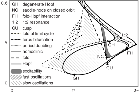
Figure 1: Bifurcation diagram for the two-section laser investigated in [6]. The parameters are: $l_{2}=1.136$, $r_{0}=10^{-5}$, $r_{L}=\eta e^{i\varphi}$, $d_{1}=-0.275$, $\kappa_{1}=3.96$, $\tilde{g}_{1}=2.145$ (linear gain model), $\alpha_{1}=5$, $\rho_{1}=0.44$, $\Gamma_{1}=90$, $\Omega_{r,1}=-20$, $I_{1}=6.757\cdot 10^{-3}$, $\tau_{1}=359$, $\dot{n}_{2}=\kappa_{2}=\beta_{2}=\rho_{2}=0$. The bifurcation parameters are the strength $\eta$ and the phase $\varphi$ of the feedback from the facet $r_{L}$ of section $S_{2}$. In the experiment these parameters can be varied by changing the current in $S_{2}$. The highlighted dynamical regimes are of particular practical interest.

Delay-differential equations

Theorem 7 also applies to systems of delay-differential equations (DDEs) as they are widely used in laser dynamics (such as, for example, the Lang-Kobayashi system for delayed optical feedback or two mutually coupled lasers; see [1, 2] and references therein). They also have the structure of system (1) where $E\in C([-1,0];\mathbb{C})$, and $H(n)$ is a linear delay operator. The parameter $\varepsilon$ is small if the feedback cavity is short. According to [20], $H(n)$ generates an eventually compact semigroup and, thus, the existence of critical carrier densities with a spectral gap can be shown analytically [2]. Moreover, the cut-off modification performed in the proof of Theorem 7 manipulates only the finite-dimensional components $E_{c}$ and $n$. Hence, the proof does not rely on the ability to cut-off a smooth map smoothly in the infinite-dimensional space $X$ which is the Hilbert space $X=\mathbb{L}^{2}([0,L];\mathbb{C}^{2})\times\mathbb{L}^{2}([0,L];\mathbb{C}^{2})$ in Section 6 but a Banach space for DDEs. The only property of the operator $H(n)$ used in the proof is the existence of a spectral splitting and the smooth dependence of the dominating subspace $X_{c}$ on $n$. Consequently, Theorem 7 applies to (1) if $H(n)$ is a delay operator, reducing the DDEs to low-dimensional systems of ODEs.

References

• [1] G. van Tartwijk, G. Agrawal, Laser instabilites: a modern perspective, Prog. in Quant. El. 22 (1998) 43–122.
• [2] B. Krauskopf, D. Lenstra (Eds.), Fundamental Issues of Nonlinear Laser Dynamics, American Institute of Physics, 2000.
• [3] D. Peterhof, B. Sandstede, All-optical clock recovery using multisection distributed-feedback lasers, J. Nonlinear Sci. 9 (1999) 575–613.
• [4] E. Avrutin, J. Marsh, J. Arnold, Modelling of semiconductorlaser structures for passive harmonic mode locking at terahertz frequencies, Int. J. of Optoelectronics 10 (6) (1995) 427–432.
• [5] S. Bauer, O. Brox, J. Kreissl, B. Sartorius, M. Radziunas, J. Sieber, H.-J. Wünsche, F. Henneberger, Nonlinear dynamics of semiconductor lasers with active optical feedback, Phys. Rev. E 69 (016206).
• [6] H.-J. Wünsche, O. Brox, M. Radziunas, F. Henneberger, Excitability of a semiconductor laser by a two-mode homoclinic bifurcation, Phys. Rev. Lett. 88 (023901).
• [7] O. Ushakov, S. Bauer, O. Brox, H.-J. Wünsche, F. Henneberger, Self-organization in semiconductor lasers with ultra-short optical feedback, Phys. Rev. Lett. 92 (043902).
• [8] E. J. Doedel, A. R. Champneys, T. F. Fairgrieve, Y. A. Kuznetsov, B. Sandstede, X. Wang, AUTO97, Continuation and bifurcation software for ordinary differential equations (1998).
• [9] J. Sieber, Numerical bifurcation analysis for multi-section semiconductor lasers, SIAM J. of Appl. Dyn. Sys. 1(2) (2002) 248–270.
• [10] P. Bates, K. Lu, C. Zeng, Existence and persistence of invariant manifolds for semiflows in banach spaces, Mem. Amer. Math. Soc. 135.
• [11] P. Bates, K. Lu, C. Zeng, Persistence of overflowing manifolds for semiflow, Comm. Pure Appl. Math. 52 (8).
• [12] P. Bates, K. Lu, C. Zeng, Invariant foliations near normally hyperbolic invariant manifolds for semiflows, Trans. Amer. Math. Soc. 352 (10) (2000) 4641–4676.
• [13] U. Bandelow, M. Wolfrum, M. Radziunas, J. Sieber, Impact of gain dispersion on the spatio-temporal dynamics of multisection lasers, IEEE J. of Quant El. 37 (2) (2001) 183–189.
• [14] J. Rehberg, H.-J. Wünsche, U. Bandelow, H. Wenzel, Spectral properties of a system describing fast pulsating DFB lasers, ZAMM 77 (1) (1997) 75–77.
• [15] L. Recke, K. Schneider, V. Strygin, Spectral properties of coupled wave equations, Z. angew. Math. Phys. 50 (1999) 923–933.
• [16] B. Tromborg, H. Lassen, H. Olesen, Travelling wave analysis of semiconductor lasers, IEEE J. of Quant. El. 30 (5) (1994) 939–956.
• [17] F. Jochmann, L. Recke, Well-posedness of an initial boundary value problem arising in laser dynamics, Math. Models Methods Appl. Sci. 12 (4) (2002) 593–606.
• [18] A. Pazy, Semigroups of Linear Operators and Applications to Partial Differential Equations, Applied mathematical Sciences, Springer Verlag, New York, 1983.
• [19] A. Neves, H. Ribeiro, O. Lopes, On the spectrum of evolution operators generated by hyperbolic systems, Journal of Functional Analysis 67 (1986) 320–344.
• [20] O. Diekmann, S. van Gils, S. V. Lunel, H.-O. Walther, Delay Equations, Vol. 110 of Applied Mathematical Sciences, Springer-Verlag, 1995.
• [21] U. Bandelow, Theorie longitudinaler Effekte in 1.55 $\mu$m Mehrsektions DFB-Laserdioden, Ph.D. thesis, Humboldt-Universität Berlin (1994).
• [22] D. Turaev, Fundamental obstacles to self-pulsations in low-intensity lasers, Preprint 629, WIAS, submitted to SIAM J. of Appl. Math (2001).
• [23] N. Fenichel, Geometric singular perturbation theory for ordinary differential equations, Journal of Differential Equations 31 (1979) 53–98.
• [24] U. Bandelow, L. Recke, B. Sandstede, Frequency regions for forced locking of self-pulsating multi-section DFB lasers, Opt. Comm. 147 (1998) 212–218.
• [25] H. Triebel, Interpolation Theory, Function Spaces, Differential Operators, N.-Holland, Amsterdam-New-York, 1978.
• [26] U. Bandelow, H. J. Wünsche, B. Sartorius, M. Möhrle, Dispersive self Q-switching in DFB lasers: theory versus experiment, IEEE J. Selected Topics in Quantum Electronics 3 (1997) 270–278.
• [27] J. Sieber, Numerical bifurcation analysis for multi-section semiconductor lasers, Preprint 683, WIAS, to appear in SIAM J. of Appl. Dyn. Sys. (2001).
• [28] H. Wenzel, U. Bandelow, H.-J. Wünsche, J. Rehberg, Mechanisms of fast self pulsations in two-section DFB lasers, IEEE J. of Quant. El. 32 (1) (1996) 69–79.
• [29] M. Radziunas, H.-J. Wünsche, Dynamics of multi-section DFB semiconductor laser: traveling wave and mode approximation models, Preprint 713, WIAS, submitted to SPIE (2002).
• [30] M. Wolfrum, D. Turaev, Instabilities of lasers with moderately delayed optical feedback, Preprint 714, WIAS, submitted to Opt. Comm. (2002).