A Scaling Theory for ac Magnetic Response in Kagomé Ice

Abstract

A theory for frequency-dependent magnetic susceptibility $\chi(\omega)$ is developed for thermally activated magnetic monopoles in kagomé ice. By mapping this system to a two-dimensional (2D) Coulomb gas and then to a sine-Gordon model, we have shown that the susceptibility has a scaling form $\chi(\omega)/\chi(0)={\cal F}(\omega/\omega_{1})$, where the characteristic $\omega_{1}$ is related to a charge correlation length between diffusively moving monopoles, and to the sine-Gordon principal breather. The dynamical scaling is universal among superfluid and superconducting films, and 2D XY magnets above Kosterlitz-Thouless transitions.

Frustrated spin systems have attracted considerable attention for decades, because they provide an opportunity of uncovering novel phases and excitations Lacrox11 . Even in the simplest cases of the Ising antiferromagnets on triangular Wann50 and kagomé Shozi51 lattices, exact solutions revealed the absence of magnetic order and the macroscopic degeneracy in the ground states, which are viewed as the hallmark of the frustration.

Rare-earth pyrochlore oxides such as Ho₂Ti₂O₇ Harr97 and Dy₂Ti₂O₇ Rami99 proffers a new paradigm in this research area Bram01 . It is considered that despite large magnetic moments $\mu_{\rm eff}\sim 10\mu_{\rm B}$ the spins on the pyrochlore lattice do not order down to a quite low temperature $\sim 0.1$ K Harris98b ; Bram01 , and exhibit a residual entropy Rami99 (although possibilities of a magnetic order Melk01 and an absence of the residual entropy Poma13 have been reported). The origin of these behaviors can be attributed to a strong Ising anisotropy with respect to the local $\langle 111\rangle$ axis and an effective ferromagnetic coupling between neighboring spins Hert00 , which, then, force the spins at four corners of each tetrahedron to satisfy the two-in and two-out condition. Since this constraint is the same as that for proton configurations in water ice Bern33 , those materials are named as “spin ice”.

Recently, point-defect excitations in spin ice created by breaking the ice rule Ryzh05 have been intensively investigated Kado09 ; Morris09 ; Fennell09 ; Bovo13 , since the intriguing prediction of magnetic monopoles Cast08 ; Cast11 . These excitations behave as quasi-particles with magnetic charges moving on the diamond lattice Ryzh05 ; Bram09 ; Gibl11 like ion defects, H₃O⁺ and HO^-, in water ice Bjer51 . While much efforts have been paid to account for their static and dynamical properties, there still exist unclear points and subjects to explore Bram12 . This is partly because the monopole-like excitation is a topological defect, and is a nonlocal object emerging in the vicinity of the ground-state manifold.

A way to circumvent its intractability is to make it move in more restricted space, e.g., in two dimensional (2D) space. A 2D spin ice can be achieved by applying a magnetic field ${\bm{H}}_{\rm dc}$ along a [111] direction, along which the pyrochlore lattice is stacking of triangular and kagomé lattices Harr98 ; Mats02 . When the [111] field is not very high, the spins on the triangular layers are fixed parallel to the field direction at low temperatures, and consequently the spins on each kagomé layer are decoupled and remain frustrated, which endowed the name “kagomé ice” Mats02 ; Saka03 ; Hiroi03 ; Higashinaka04 ; Taba06 ; Fennell07 ; Uda02 ; Moes03 ; Isak04 . The kagomé-ice state is characterized by a magnetization plateau Mats02 ; Saka03 and a reduced residual entropy Mats02 ; Hiroi03 ; Higashinaka04 ; Uda02 ; Moes03 . In the low temperature limit $T\rightarrow 0$, it is in a Coulomb phase Henley09 with the power-law decay of spin correlations Moes03 . At low $T$, kagomé ice is characterized by a long charge correlation length $\xi$ or a small monopole density $n_{\rm m}\propto\xi^{-2}$ Moes03 ; Taba06 ; Fennell07 .

A minimal Hamiltonian for kagomé ice is a nearest-neighbor (NN) model Harr98 consisting of one kagomé layer and neighboring two triangular layers with pinned spins:

$$H_{\rm ice}=J_{\rm eff}\sum_{\langle ij\rangle}\sigma_{i}\sigma_{j}-\mu_{\rm eff}\sum_{i}{\bm{H}}_{\rm dc}\cdot\hat{\bm{z}}_{a(i)}\sigma_{i}~{}~{}(J_{\rm eff}>0).$$ (1)

$\sigma_{i}$ ($=\pm 1$) is an Ising variable for a spin ${\bm{S}}_{i}=\sigma_{i}\hat{\bm{z}}_{a(i)}$ at a site $i$ on a sublattice $a(i)$, and $\hat{\bm{z}}_{a(i)}$ stands for a unit vector parallel to the local Ising axis. The NN exchange interaction is antiferromagnetic in terms of Ising variables. The ice rule, requiring $\sum_{a=1}^{4}\sigma_{a}=0$ for each tetrahedron, can be broken by thermal activation, creating magnetic monopoles with a charge $q=\frac{1}{2}\sum_{a=1}^{4}\sigma_{a}=\pm 1$, which is illustrated in Fig. 1.

Another motivation of this work originates from our recent experimental studies on the dynamics of monopoles moving in the kagomé plane of Dy₂Ti₂O₇ Takatsu13 : As pointed out there, the 2D dynamics of monopoles excited from the kagomé-ice state can be investigated by applying an ac magnetic field ${\bm{H}}_{\rm ac}(t)={\rm Re}[{\bm{H}}_{0}e^{i\omega t}]$ perpendicular to ${\bm{H}}_{\rm dc}$, which works as driving force for monopoles and measuring induced magnetization ${\bm{M}}_{\rm ac}(t)={\rm Re}[\chi(\omega){\bm{H}}_{0}e^{i\omega t}]$. The frequency-dependent ac susceptibility $\chi(\omega)$ has been indeed measured. In the low-frequency ranges of the experiments Snyder01 ; Matsu01 ; Takatsu13 , the monopole motion is thought to be governed by diffusion Jaub09 , characterized by a diffusion constant ${\cal D}$.

In this letter, we have theoretically studied $\chi(\omega)$, and have found that it gives deep insight into the monopole dynamics in the kagomé-ice state. Using the monopole degrees of freedom, kagomé ice can be mapped to the 2D Coulomb gas model Minn87 , in which monopoles interact via the logarithmic Coulomb potential, which is caused by the entropic interaction in kagomé ice Moes03 ; Isak04 . The dynamical properties of the 2D Coulomb gas were closely discussed Ambe78 ; Minn87 , as the vortex dynamics in the superfluid films Bish77 . Based on the sine-Gordon theory Minn87 ; Poly77 , we have shown that $\chi(\omega)$ is expressed by a scaling form

$$\chi(\omega)/\chi(0)\simeq{\cal F}(\omega/\omega_{1}),$$ (2)

where $\omega_{1}={\cal D}/\xi^{2}$ is a characteristic frequency of kagomé ice (see below). It is expected that the scaling function ${\cal F}$ shown in Fig. 2 can be used to analyze experimental data on the 2D spin ice systems. We note that this scaling is universal in the sense that it is applicable not only for kagomé ice, but also for other systems: superfluid and superconducting films Bish77 , 2D XY magnets above the Kosterlitz-Thouless transition Kosterlitz ; Kost74 , and generic 2D ices possibly including the artificial spin ice Wang06 ; Mengotti11 ; Farhan13 ; Wills02 ; Chern11 ; Moller11 .

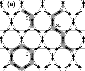
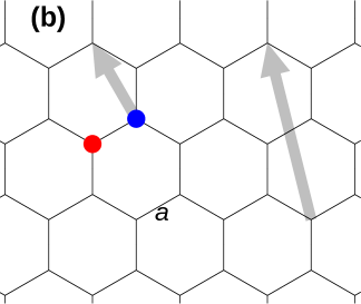
Figure 1: (Color online) Spin (monopole) configurations on $\Lambda^{*}$ ($\Lambda$) are given in (a) and (c) [(b) and (d)]. (a) The loop (${\cal C}$) and strings (${\cal S}_{1,2}$) are given by thick gray lines along which spins line up tail to nose. (b) The red (blue) circle represents a positive (negative) charge monopole; $a$ indicates the site spacing. Thick gray arrows show the displacements.

First, we address Ryzhkin’s argument which provides a link between the magnetization ${\bm{M}}=\mu_{\rm eff}\sum_{l^{*}\in\Lambda^{*}}{\bm{S}}_{l^{*}}$ and a polarization of the monopole charge distribution ${\bm{P}}=(2\mu_{\rm eff}/a)\sum_{l\in\Lambda}q_{l}{\bm{x}}_{l}$ Ryzh05 . The sum runs over all sites $l^{*}$ ($l$) in the kagomé (honeycomb) lattice $\Lambda^{*}$ ($\Lambda$). The factor, $2\mu_{\rm eff}/a$, is for later convenience, and $a$ is the site spacing of $\Lambda$. Note that, we henceforth focus on one kagomé layer. In Figs. 1(a) and 1(b), we sketch a spin configuration and the corresponding monopole charge distribution. The monopole on the ${\cal A}$ (${\cal B}$) sublattice is viewed as a particle with positive (negative) charge $q_{l}=\pm 1$. To demonstrate a link, we consider changes in ${\bm{M}}$ and ${\bm{P}}$ caused by a directed loop flip of spins along ${\cal C}$ and string flips of spins along ${\cal S}_{1}$ and ${\cal S}_{2}$. While the loop flip (and also any loop flips) does not change them, the string flip along ${\cal S}_{1}$ makes the monopole hop from one end to another [see Figs. 1(b) and 1(d)]. Since the displacement is given by the vector sum of spins associated, the change in ${\bm{M}}$ equals to that in ${\bm{P}}$, due to the front factor. Moreover, the same relation, $\delta{\bm{M}}=\delta{\bm{P}}$, holds for the string flip along ${\cal S}_{2}$ which newly creates a pair of monopoles connected by ${\cal S}_{2}$ [see Fig. 1(d)]. The time derivative of the polarization equals to the monopole current ${\bm{J}}=\dot{\bm{P}}$, so these observations lead to Ryzhkin’s relation ${\bm{J}}=\dot{\bm{M}}$. In order further to explore their link, let us consider the vacuum of monopoles. Although ${\bm{P}}=0$ by definition, there exist spin configurations with ${\bm{M}}\neq 0$ belonging to nonzero winding-number sectors. In spite of this, we shall approximate ${\bm{M}}\simeq{\bm{P}}$ because the volume of spin configurations with ${\bm{M}}=0$ which includes the maximally-flippable state Moes00 is expected to comprise a major portion of the ground-state manifold. Therefore, we will focus on a magnetic response accompanied by creations, annihilations and rearrangements of monopoles: $\chi=\frac{1}{2{k_{\rm B}T}}\langle{\bm{M}}^{2}\rangle_{\rm ice}\simeq\frac{1}{2{k_{\rm B}T}}\langle{\bm{P}}^{2}\rangle_{\rm ice}$ Jaub12 .

Since kagomé ice exhibits an isotropic charge correlation, we rewrite $\chi$, by introducing the charge-density distribution function $\rho({\bm{x}})=\sum_{l\in\Lambda}q_{l}\delta({\bm{x}}-{\bm{x}}_{l})$, as

$$\chi=\Omega\frac{\pi\mu^{2}_{\rm eff}}{{k_{\rm B}T}a^{2}}\int_{0}^{\infty}dr~{}r^{3}C(r),$$ (3)

where $r=|{\bm{x}}|$ and $\Omega$ is the area of $\Lambda$. The charge correlation function was defined as $C(r)=-\langle\rho({\bm{x}})\rho({\bf 0})\rangle_{\rm ice}$.

Equation (3) exhibits the magnetic response in terms of monopole degrees of freedom. However, it is restricted to the static case, so its extension to the dynamical case is our next task. For this purpose, second, we address Ambegaokar’s argument, which provides a link between the ac response and a static charge correlation Ambe78 . In the analysis of the superfluid film on the oscillating substrate, Ambegaokar et al. supposed a diffusive motion of vortices, and then obtained the ac response by focusing on a role of the mean diffusion length during a period of an ac field $L_{\omega}=\sqrt{{\cal D}/\omega}$. One intuitive reasoning is as follows: Consider a pair of monopoles with separation $r$, and suppose its time-dependent polarization keeping in phase with the ac field. Then, a monopole should move a distance of order of the separation during one ac period, while the mean diffusion length gives a reachable distance by diffusive motion within one period. Thus, in order to give the in-phase response, the pair should satisfy a condition $r<O(L_{\omega})$ Minn87 . Here, we also assume a diffusive motion and apply this heuristic argument to express the in-phase component (real part) $\chi^{\prime}(\omega)$ of $\chi(\omega)$. The result is given by replacing the upper bound of the integral in Eq. (3) with the length of $O(L_{\omega})$:

$$\chi^{\prime}(\omega)\simeq\Omega\frac{\pi\mu^{2}_{\rm eff}}{k_{\rm B}Ta^{2}}\int_{0}^{bL_{\omega}}dr~{}r^{3}C(r).$$ (4)

We have introduced a constant $b$ less than order of unity. In order to infer the value of $b$, we assume a uni-dimensional motion of monopoles parallel to ${\bm{H}}_{\rm ac}$. Then, the round-trip path length of monopoles is about $4r$ so that the condition $4r<L_{\omega}$ is satisfied. We thus assume $b=\frac{1}{4}$ AmbeTeit79 . The imaginary part $\chi^{\prime\prime}(\omega)$ is obtained by applying the Kramers-Kronig (KK) relation to $\chi^{\prime}(\omega)$. The above formula is doubly important: It gives the magnetic response in terms of the charge correlation, which is possible only for magnets to afford their defect representations like the monopole system for kagomé ice. Also, since the frequency dependence is introduced as a finite-size effect, it may be governed by a ratio of $L_{\omega}$ to the characteristic length $\xi$ in kagomé ice. Below, one can see that this is indeed an origin of a scaling nature of $\chi(\omega)$.

Now, we can obtain $\chi(\omega)=\chi^{\prime}(\omega)-i\chi^{\prime\prime}(\omega)$ via $C(r)$, which is given as an average with respect to $H_{\rm ice}$. This is rather convenient for numerical calculations; in fact, we perform Monte Carlo simulations to evaluate Eq. (4). However, to analytically evaluate $\chi(\omega)$, a monopole representation of $H_{\rm ice}$ is necessary. It has been argued that a gaseous model gives its effective description

$$H_{\rm CG}=k_{\rm B}T\sum_{l,m\in\Lambda;l>m}-q_{l}q_{m}g(|{\bm{x}}_{l}-{\bm{x}}_{m}|)\kappa,$$ (5)

where a neutrality condition $\sum_{l\in\Lambda}q_{l}=0$ is imposed Isak04 . $g(r)$ is a lattice propagator to give the correlation between two monopoles with a separation $r$ in the ground-state manifold, and represents an entropic interaction. Since we are focusing on the system with a long correlation length $\xi\propto 1/\sqrt{n}_{\rm m}$, the interaction can be approximated by its asymptotic behavior $\ln(r/a_{0})$, where $a_{0}$ is a monopole core radius. In this dilute-gas regime, we can obtain a simple universal system by coarse-graining a lattice structure and neglecting short-range fluctuations Kost74 : Equation (5) defines the 2D coulomb-gas (CG) model Kadanoff , where $\kappa$ is the inverse CG temperature, and is independent of $T$ ($\kappa\simeq\frac{1}{2}$ for an ice-rule system Fish63 ).

A large reduction of the problem has been attained, but as its drawbacks, we should explicitly control a number of monopoles. Let us write a $N$-monopole partition function as $Z_{N}$, then the grand-partition function is given as $\Xi_{\rm CG}=\sum_{N:{\rm even}}y^{N}Z_{N}$, where the fugacity $y=e^{-\Delta/k_{\rm B}T}$. $\Delta$ is a monopole creation energy, which is, to some extent, controlled by ${\bm{H}}_{\rm dc}$. Then, we can estimate the asymptotic behavior of the charge correlation function as $C(r)\simeq-\langle\rho({\bm{x}})\rho({\bf 0})\rangle_{\rm CG}$, where $\langle\cdots\rangle_{\rm CG}$ means an average with respect to $\Xi_{\rm CG}$.

While CG possesses a low-temperature phase ($\kappa\geq 4$) where monopoles with opposite charges are bounded into pairs Kost74 , kagomé ice corresponds to CG in the high-temperature phase ($\kappa\simeq\frac{1}{2}$), and thus, exhibits a screened charge correlation due to free monopoles. To evaluate $C(r)$, we utilize the well-known equivalence between CG and the sine-Gordon model Minn87 ; Poly77 defined by the partition function $Z_{\rm sG}=\int[d\vartheta]e^{-{\cal S}_{\rm sG}}$ with the action Otsu11 :

$${\cal S}_{\rm sG}=\int d^{2}x\Bigl{[}\frac{1}{2\pi\kappa}\left(\nabla\vartheta\right)^{2}-2z\cos\sqrt{2}\vartheta\Bigr{]},$$ (6)

where $z\simeq(y/\zeta)a_{0}^{\kappa/2}$ ($\zeta$ is an area of unit cell of $\Lambda$). Then, in the sine-Gordon language, $C(r)=4z^{2}c(r)$ $(r\neq 0)$ with

$$c(r)=\langle\sin\sqrt{2}\vartheta({\bm{x}})\sin\sqrt{2}\vartheta({\bf 0})\rangle_{\rm sG},$$ (7)

where $\langle\cdots\rangle_{\rm sG}$ means an average with respect to $Z_{\rm sG}$. In this formulation, $c(r)$ is short-ranged due to the relevant nonlinear term in Eq. (6). In such cases, it can be calculated reliably by using the formfactor perturbation (FFP) method. While the method tells us elementary processes to be considered and provides a simple expression for $c(r)$, its explanation is devoted to a rather technical aspect of the massive sine-Gordon theory. Thus, here we only provide the result—for readers interested in details, please see the Supplementary Material (SM):

$$c(r)\simeq\left(\frac{\lambda n_{\rm m}}{2z}\right)^{2}\frac{K_{0}(m_{1}r)}{\pi},$$ (8)

where $K_{\alpha}$ denotes the $\alpha$th-order modified Bessel function of the second kind. Thus, $C(r)$ is short-ranged with $\xi=1/m_{1}$, where $m_{1}$ is the mass of the principal breather $B_{1}$.

Now, we are in a position to obtain the ac susceptibility. Performing the integral transform of Eq. (4) CALTECH , we obtain the real part as

$${\chi^{\prime}(\omega)}/{\chi(0)}\simeq 1-\frac{\gamma^{3}}{8}\left[K_{1}(\gamma)+K_{3}(\gamma)\right].$$ (9)

We defined a characteristic frequency of the $B_{1}$ excitation (see SM) as $\omega_{1}={\cal D}/\xi^{2}$ and a ratio as $\gamma=bL_{\omega}/\xi=b\sqrt{\omega_{1}/\omega}$. The static susceptibility $\chi$ $[=\chi(0)]$ which gives a magnitude of $\chi(\omega)$ is found to obey Curie’s law:

$$\chi(0)\simeq\Omega\frac{4\mu^{2}_{\rm eff}}{k_{\rm B}Ta^{2}}\lambda^{2}n_{\rm m}^{2}\xi^{4}=\frac{\cal C}{k_{\rm B}T}.$$ (10)

Intriguingly, Curie’s constant depends on $\kappa$ characterizing the ground-state manifold (${\cal C}\simeq 0.55\times\mu^{2}_{\rm eff}N_{\Lambda^{*}}$ for $\kappa=\frac{1}{2}$ and $N_{\Lambda^{*}}$ spins), which may give one aspect of the 2D cooperative paramagnets. The imaginary part is obtained by the KK relation; the result is written, in terms of Meijer’s $G$ functions Meij36 , as

$${\chi^{\prime\prime}(\omega)}/{\chi(0)}\simeq\frac{\gamma^{2}}{8\pi}\Bigl{[}G_{1,5}^{4,1}\Bigl{(}\frac{\gamma^{4}}{2^{8}}\Bigl{|}\genfrac{}{}{0.0pt}{}{\lower 2.27621pt\hbox{0}}{\raise 0.85358pt\hbox{{\bf a}}}\Bigr{)}-G_{1,5}^{4,1}\Bigl{(}\frac{\gamma^{4}}{2^{8}}\Bigl{|}\genfrac{}{}{0.0pt}{}{\lower 2.27621pt\hbox{0}}{\raise 0.85358pt\hbox{{\bf b}}}\Bigr{)}\Bigr{]},$$ (11)

where vectors ${\bf a}=(0,0,1,\frac{3}{2},-\frac{1}{2})$ and ${\bf b}=(0,0,\frac{1}{2},1,\frac{1}{2})$.

Before exploring ingredients of Eqs. (9)–(11), two comments are in order: (i) Because we have focused in the vicinal region from the ground-state manifold of kagomé ice, the temperature should not be so high to bring the system out of the region. Moreover, ${\bm{H}}_{\rm dc}$ should be at least in the interval to give the magnetization plateau. (ii) The FFP expansion provides an efficient approximation for the long-distance behavior of $c(r)$, but it is not for the short-distance one. Despite of this fact, we expect it to work at least in the low-frequency (i.e., long-distance) region because the $r^{3}$ factor in Eq. (4) relatively amplifies the contribution from the long-distance part of the charge correlation.

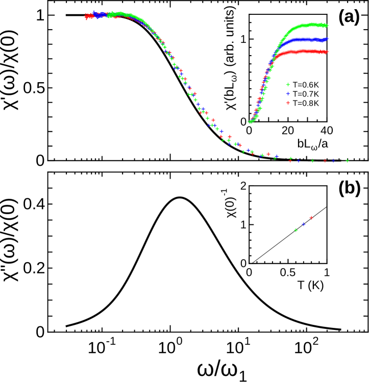
Figure 2: (Color online) The ac susceptibility: (a) Eq. (9) and (b) Eq. (11). The frequency is given in units of $\omega_{1}$, and is plotted on a logarithmic scale, where $b=\frac{1}{4}$ (see text). The cut-off dependence of $\chi^{\prime}$ obtained by MC simulations are given in the inset of (a); the value $1/\chi(0)$ is plotted in the inset of (b), where a fitting line is also given by using data at the lowest two temperatures. The scaled MC simulation data using monopole density and $\chi(0)$ are given in (a).

In Fig. 2, we give Eqs. (9) and (11) by the solid lines. Since $\omega$ is always scaled by $\omega_{1}$, these curves are independent of model parameters. However, it is, strictly speaking, due to the single-mode approximation in the FFP expansion; thus, the corrections to scaling may possibly be expected. In this plot, one finds that $\chi^{\prime}(\omega)$ exhibits a steep decrease at around $\omega_{1}$, where $\chi^{\prime\prime}(\omega)$ forms an asymmetric peak. Therefore, $B_{1}$ is responsible for the in-phase component, and its delay in response against ${\bm{H}}_{\rm ac}(t)$ causes a dephasing, which is then detected as the peak in $\chi^{\prime\prime}(\omega)$. The frequency $\omega_{1}$ is the square of the $B_{1}$ mass, so it increases as a power of $z$ with the exponent $1+p$ (see SM). Thus, with increasing $z$, but keeping $T$ constant, the peak shifts toward higher frequency region according to the power law, but its height is almost unchanged (if ${\cal D}$ is a constant). We expect that these behaviors as well as the scaling properties give a hallmark of the ac magnetic response observed in the 2D spin ice.

Finally, we perform Monte Carlo (MC) simulations of kagomé ice by using the NN model of $H_{\rm ice}$ with $J_{\rm eff}=4.4$ K Harr97 ; Taba06 ; Melk01 . We employ a system of $54\times 54$ pairs of tetrahedra, and simulate it at $|{\bm{H}}_{\rm dc}|=0.3$ T and $T=0.6$, 0.7 and 0.8 K, where Dy₂Ti₂O₇ is known to be in the kagomé-ice state Taba06 . We estimate $n_{\rm m}$ and $C(r)$ by MC simulations. Since the sublattice dependence of $q_{l}$ in the lattice model hinders detection of large-scale behavior of $C(r)$, we performed a coarse graining of charge distributions using the unit cell of $\Lambda$. We summarize our simulation results in Fig. 2(a). One can find that scaled data of different $T$ (and thus $n_{\rm m}$) given by marks with error bars agree with the theoretical curve. This fact suggests that our theory is applicable for the ac magnetic response in kagomé ice. The inset of Fig. 2(a) gives the $bL_{\omega}$ dependence of $\chi^{\prime}$ defined by Eq. (4), which exhibits a saturation to a static value $\chi(0)$. Further, $\xi$ can be evaluated from $n_{\rm m}$ (see SM). Therefore, we can plot the MC simulation data as functions of $\omega/\omega_{1}$ $[=(\xi/L_{\omega})^{2}]$. In the inset of Fig. 2(b), we plot $1/\chi(0)$ versus $T$. Although we have predicted Curie’s law, a small deviation is visible. This may be due to the finite-size effects in low $T$ region, but more intensive numerical simulations are necessary for the kagomé-ice model.

In conclusion, we have investigated the ac susceptibility $\chi(\omega)$ of kagomé ice: We clarified that $\chi(\omega)$ takes an universal scaling form in terms of the ratio of $\omega$ to $\omega_{1}$, the characteristic frequency for the principal breather— it is a localized excitation composed of a soliton and antisoliton, but possibly looks more similar to an ordinary wave Sasa86 . Furthermore, we performed MC simulations, and provided data that represent the scaling form as expected in our theory. The present results suggest that breather’s dynamics characterizes the low-$T$ behavior of the magnetic monopoles in kagomé ice. In this letter, it has been explained that the universal dynamics of the magnetic monopole-like defects in the 2D spin ice can be captured by the theory of the ac magnetic response. Now, in view of the universality concept, it is natural to expect that our theory can also serve for analysis of the dynamics observed in other systems such as the vortices in superfluid and superconducting films, as well as in 2D XY magnets above the Kosterlitz-Thouless transition, and also the charged particles in 2D electrolytes. These remain as interesting future applications.

The authors thank Y. Okabe, G. Tatara, M. Fujimoto, A. Tanaka, and K. Nomura for stimulating discussions. Main computations were performed using the facilities of Cyberscience Center in Tohoku University.

This Supplementary Material contains an explanation on the formfactor perturbation (FFP) calculation of the charge correlation function defined by Eq. (7) and its lowest-order result given by Eq. (8) Smir92 . Also, a relationship between the charge correlation length and the defect number density is obtained as a by-product.

The model Eq. (6) possesses low-energy excitations of the soliton $s$, the antisoliton $\bar{s}$, and breathers $B_{j}$ for $0\leq\kappa<2$ ($j=1,\cdots,\lfloor 1/p\rfloor$ with $1/p=4/\kappa-1$) Fadd74 ; Zamo79 . The mass spectrum $m_{\epsilon}$ consists of a doublet of $s$ and $\bar{s}$, $m_{\pm}=M$, and singlets of $B_{j}$,

$$m_{j}=2M\sin\left(\frac{\pi p}{2}j\right).$$ (S1)

The soliton mass varies as a power of the scaling field $z$ Dest91 ; Zamo95 :

$$M=\frac{2\Gamma(p/2)}{\sqrt{\pi}\Gamma((1+p)/2)}\left[\pi\frac{\Gamma(1/(1+p))}{\Gamma(p/(1+p))}z\right]^{\frac{1+p}{2}},$$ (S2)

and represents an inverse length scale ($M\simeq 6.22\times z^{\frac{4}{7}}$ for $\kappa=\frac{1}{2}$). The FFP method expands the correlation function as $c(r)=\sum_{{\cal N}=1}^{\infty}c_{\cal N}(r)/{\cal N}!$, where the contribution from the ${\cal N}$-excitation sector is given by

$$c_{\cal N}(r)=\prod_{k=1}^{\cal N}\Bigl{[}\sum_{\epsilon_{k}}\int_{-\infty}^{\infty}\frac{d\theta_{k}}{2\pi}e^{-E_{k}(\theta_{k})r}\Bigr{]}\Bigl{|}F_{\sin}(\{\theta\})_{\{\epsilon\}}\Bigl{|}^{2}.$$ (S3)

The two sets $\{\epsilon\}=\{\epsilon_{1},\cdots,\epsilon_{\cal N}\}$ and $\{\theta\}=\{\theta_{1},\cdots,\theta_{\cal N}\}$ specify aforementioned species of excitations and their rapidities, respectively. An $\epsilon_{k}$ excitation with a rapidity $\theta_{k}$ has the energy $E_{k}(\theta_{k})=m_{\epsilon_{k}}\cosh\theta_{k}$. The formfactor, $F_{\sin}(\{\theta\})_{\{\epsilon\}}$, represents a matrix element of $\sin\sqrt{2}\vartheta$ between the ground state and excited states, and selects relevant excitations to the correlation function. In this respect, the invariance of Eq. (6), under the charge conjugation ${\cal C}:$ $\vartheta\to-\vartheta$ has the central importance Essl97 . Since the charge-density operator transforms as ${\cal C}:$ $\sin\sqrt{2}\vartheta\to-\sin\sqrt{2}\vartheta$, nonvanishing contributions stem from excitations with odd parity. Consequently, the leading contribution comes from the principal breather $B_{1}$ which is taken into account in the expansion, i.e., ${\cal N}=1$ and $\epsilon_{1}=1$ in Eq. (S3). The formfactor is then independent of the rapidity, and is given by $F_{\sin}(\theta_{1})_{1}=-\lambda\langle e^{i\sqrt{2}\vartheta}\rangle_{\rm sG}=-\lambda n_{\rm m}/2z$ Luky95 , where the constant

$$\lambda=2\cos\frac{\pi p}{2}\sqrt{2\sin\frac{\pi p}{2}}\exp\Bigl{(}-\int_{0}^{\pi p}\frac{tdt}{2\pi\sin t}\Bigr{)},$$ (S4)

and the defect number density Luky97 ; Sama00

$$n_{\rm m}=\frac{(1+p)}{4}\tan\left(\frac{\pi p}{2}\right)M^{2}.$$ (S5)

As a result, the charge correlation function is simply given by Eq. (8). Since its asymptotic behavior in $r\to\infty$ can be written as $c(r)\propto\exp(-m_{1}r)/\sqrt{r}$, the charge correlation length $\xi=1/m_{1}$. Therefore, from Eqs. (S1) and (S5), we obtain the relationship between $\xi$ and $n_{\rm m}$ as

$$\xi^{-1}=\sqrt{\frac{8n_{\rm m}}{1+p}\sin(\pi p)}.$$ (S6)

For instance, $\xi^{-1}=\sqrt{7n_{\rm m}\sin(\pi/7)}$ for $\kappa=\frac{1}{2}$.

References

- (1) C. Lacroix, P. Mendels, and F. Mila, eds., Introduction to Frustrated Magnetism (Springer, 2011).
- (2) G.H. Wannier, Phys. Rev. 79, 357 (1950); Phys. Rev. B 7, 5017 (1973).
- (3) I. Syôzi, Prog. Theor. Phys. 6, 306 (1951).
- (4) M.J. Harris, S.T. Bramwell, D.F. McMorrow, T. Zeiske, and K.W. Godfrey, Phys. Rev. Lett. 79, 2554 (1997).
- (5) A.P. Ramirez, A. Hayashi, R.J. Cava, R. Siddharthan, and B.S. Shastry, Nature 399, 33 (1999).
- (6) S.T. Bramwell and M.J.P. Gingras, Science 294, 1495 (2001).
- (7) R.G. Melko, B.C. den Hertog, and M.J.P. Gingras, Phys. Rev. Lett. 87, 067203 (2001).
- (8) D. Pomaranski, L.R. Yaraskavitch, S. Meng, K.A. Ross, H.M.L. Noad, H.A. Dabkowska, B.D. Gaulin, and J.B. Kycia, Nat. Phys. 9, 353 (2013).
- (9) M.J. Harris, S.T. Bramwell, T. Zeiske, D.F. McMorrow, and P.J.C. King, J. Magn. Magn. Mater. 177, 757 (1998).
- (10) B.C. den Hertog and M.J.P. Gingras, Phys. Rev. Lett. 84, 3430 (2000).
- (11) J.D. Bernal and R.H. Fowler, J. Chem. Phys. 1, 515 (1933).
- (12) I.A. Ryzhkin, J. Exp. Theory Phys. 101, 481 (2005).
- (13) H. Kadowaki, N. Doi, Y. Aoki, Y. Tabata, T.J. Sato, J.W. Lynn, K. Matsuhira, and Z. Hiroi, J. Phys. Soc. Jpn. 78, 103706 (2009).
- (14) D.J.P. Morris, D.A. Tennant, S.A. Grigera, B. Klemke, C. Castelnovo, R. Moessner, C. Czternasty, M. Meissner, K.C. Rule, J.-U.Hoffmann, K. Kiefer, S. Gerischer, D. Slobinsky, and R.S. Perry, Science 326, 5951 (2009).
- (15) T. Fennell, P.P. Deen, A.R. Wildes, K. Schmalzl, D. Prabhakaran, A.T. Boothroyd, R.J. Aldus, D.F. McMorrow, and S.T. Bramwell, Science 326, 415 (2009).
- (16) L. Bovo, J.A. Bloxsom, D. Prabhakaran, G. Aeppli, and S.T. Bramwell, Nat. Commun. 4, 1535 (2013).
- (17) C. Castelnovo, R. Moessner, and S.L. Sondhi, Nature 451, 42 (2008).
- (18) See also, C. Castelnovo, R. Moessner, and S.L. Sondhi, Phys. Rev. B 84, 144435 (2011).
- (19) S.T. Bramwell, S.R. Giblin, S. Calder, R. Aldus, D. Prabhakaran, and T. Fennell, Nature 461, 956 (2009).
- (20) S.R. Giblin, S.T. Bramwell, P.C. W. Holdsworth, D.Prabhakaran, and I. Terry, Nat. Phys. 7, 252 (2011).
- (21) K. Bjerrum, K. Dan. Vidensk. Selsk. Mat.-Fys. Medd. 27, 1 (1951).
- (22) S.T. Bramwell, Phil. Trans. R. Soc. A 370, 5738 (2012).
- (23) M.J. Harris, S.T. Bramwell, P.C.W. Holdsworth, and J.D.M. Champion, Phys. Rev. Lett. 81, 4496 (1998).
- (24) K. Matsuhira, Z. Hiroi, T. Tayama, S. Takagi, and T. Sakakibara, J. Phys. Condens. Matter 14, L559 (2002).
- (25) T. Sakakibara, T. Tayama, Z. Hiroi, K. Matsuhira, and S. Takagi, Phys. Rev. Lett. 90, 207205 (2003).
- (26) Z. Hiroi, K. Matsuhira, S. Takagi, T. Tayama, and T. Sakakibara, J. Phys. Soc. Jpn. 72, 411 (2003).
- (27) R. Higashinaka, H. Fukazawa, K. Deguchi, and Y. Maeno, J. Phys. Soc. Jpn. 73, 2845 (2004).
- (28) Y. Tabata, H. Kadowaki, K. Matsuhira, Z. Hiroi, N. Aso, E. Ressouche, and B. Fåk, Phys. Rev. Lett. 97, 257205 (2006).
- (29) T. Fennell, S.T. Bramwell, D.F. McMorrow, P. Manuel, and A.R. Wildes, Nat. Phys. 3, 566 (2007).
- (30) M. Udagawa, M. Ogata, and Z. Hiroi, J. Phys. Soc. Jpn. 71, 2365 (2002).
- (31) R. Moessner and S.L. Sondhi, Phys. Rev. B 68, 064411 (2003).
- (32) S.V. Isakov, K.S. Raman, R. Moessner, and S.L. Sondhi, Phys. Rev. B 70, 104418 (2004).
- (33) C.L. Henley, Annu. Rev. Condens. Matter Phys. 1, 179 (2010).
- (34) H. Takatsu, K. Goto, H. Otsuka, R. Higashinaka, K. Matsubayashi, Y. Uwatoko, and H. Kadowaki, J. Phys. Soc. Jpn. 82, 073707 (2013).
- (35) J. Snyder, J.S. Slusky, R.J. Cava, and P. Schiffer, Nature 413, 48 (2001).
- (36) K. Matsuhira, Y. Hinatsu, and T. Sakakibara, J. Phys.: Condens. Matter 13, L737 (2001).
- (37) L.D.C. Jaubert and P.C.W. Holdsworth, Nat. Phys. 5, 258 (2009); J. Phys.: Condens. Matter 23, 164222 (2011).
- (38) P. Minnhagen, Rev. Mod. Phys. 59, 1001 (1987).
- (39) V. Ambegaokar, B.I. Halperin, D.R. Nelson, and E.D. Siggia, Phys. Rev. Lett. 40, 783 (1978).
- (40) D. Bishop and J. Reppy, Bull. Am. Phys. Soc. 22, 638 (1977).
- (41) A.M. Polyakov, Nucl. Phys. B 120, 429 (1977).
- (42) J.M. Kosterlitz and D.J. Thouless, J. Phys. C 6, 1181 (1973).
- (43) J.M. Kosterlitz, J. Phys. C: Solid State Phys. 7, 1046 (1974).
- (44) R.F. Wang, C. Nisoli, R.S. Freitas, J. Li, W. McConville, B.J. Cooley, M.S. Lund, N. Samarth, C. Leighton, V.H. Crespi, and P. Schiffer, Nature 439, 303 (2006).
- (45) E. Mengotti, L.J. Heyderman, A.F. Rodríguez, F. Nolting, R.V. Hügli, and H.-B. Braun, Nat. Phys. 7, 68 (2011).
- (46) A. Farhan, P.M. Derlet, A. Kleibert, A. Balan, R.V. Chopdekar, M. Wyss, L. Anghinolfi, F. Nolting, and L.J. Heyderman, Nat. Phys. 9, 375 (2013).
- (47) A.S. Wills, R. Ballou, and C. Lacroix, Phys. Rev. B 66, 144407 (2002).
- (48) Gia-Wei Chern, P. Mellado, and O. Tchernyshyov, Phys. Rev. Lett. 106, 207202 (2011).
- (49) G. Möller and R. Moessner, Phys. Rev. B 80, 140409 (2009).
- (50) R. Moessner, S.L. Sondhi, and P. Chandra, Phys. Rev. Lett. 84, 4457 (2000).
- (51) For topological sector fluctuations in the coulomb phase, see L.D.C. Jaubert, M.J. Harris, T. Fennell, R.G. Melko, S.T. Bramwell, and P.C.W. Holdsworth, Phys. Rev. X 3, 011014 (2013).
- (52) See also, V. Ambegaokar and S. Teitel, Phys. Rev. B 19, 1667 (1979).
- (53) L.P. Kadanoff, Statistical Physics: Statics, Dynamics and Renormalization (World Scientific, Singapore,2000).
- (54) M.E. Fisher and J. Stephenson, Phys. Rev. 132, 1411 (1963).
- (55) H. Otsuka, Phys. Rev. Lett. 106, 227204 (2011).
- (56) A. Erdélyi et al., Tables of Integral Transforms (McGraw-Hill, New York ,1954), Vol. 2, Chap. 10.
- (57) G.S. Meijer, Nieuw. Arch. Wiskunde (2) 18, 10 (1936).
- (58) L.R. Yaraskavitch, H.M. Revell, S. Meng, K.A. Ross, H.M.L. Noad, H.A. Dabkowska, B.D. Gaulin, and J.B. Kycia, Phys. Rev. B 85, 020410(R) (2012).
- (59) K. Sasaki, Phys. Rev. B 33, 2214 (1986).
Supplementary Material:

References

-
(1)
F.A. Smirnov,
Form Factors in Completely Integrable Models of Quantum
Field Theories
(World Scientific, Singapore, 1992). - (2) L.D. Faddeev and L.A. Takhtajan, Teor. Mat. Fiz. 21, 160 (1974).
- (3) A.B. Zamolodchikov and Al.B. Zamolodchikov, Ann. Phys. (NY) 120, 253 (1979).
- (4) C. Destri and H. de Vega, Nucl. Phys. B 358, 251 (1991).
- (5) Al.B. Zamolodchikov, Int. J. Mod. Phys. A 10, 1125 (1995).
- (6) F.H.L. Essler, A.M. Tsvelik, and G. Delfino, Phys. Rev. B 56, 11001 (1997).
- (7) S. Lukyanov, Commun. Math. Phys. 167, 183 (1995); Mod. Phys. Lett. A 12, 2543 (1997).
- (8) S. Lukyanov and A. Zamolodchikov, Nucl. Phys. B 493, 571 (1997).
- (9) L. Šamaj and I. Travěnec, J. Stat. Phys. 101, 713 (2000).