Accurate expansions of internal energy and specific heat of critical two-dimensional Ising model with free boundaries

Abstract

The bond-propagation (BP) algorithm for the specific heat of the two dimensional Ising model is developed and that for the internal energy is completed. Using these algorithms, we study the critical internal energy and specific heat of the model on the square lattice and triangular lattice with free boundaries. Comparing with previous works [X.-T. Wu et al Phys. Rev. E 86, 041149 (2012) and Phys. Rev. E 87, 022124 (2013)], we reach much higher accuracy ($10^{-26}$) of the internal energy and specific heat,compared to the accuracy $10^{-11}$ of the internal energy and $10^{-9}$ of the specific heat reached in the previous works. This leads to much more accurate estimations of the edge and corner terms. The exact values of some edge and corner terms are therefore conjectured. The accurate forms of finite-size scaling for the internal energy and specific heat are determined for the rectangle-shaped square lattice with various aspect ratios and various shaped triangular lattice. For the rectangle-shaped square and triangular lattices and the triangle-shaped triangular lattice, there is no logarithmic correction terms of order higher than $1/S$, with $S$ the area of the system. For the triangular lattice in rhombus, trapezoid and hexagonal shapes, there exist logarithmic correction terms of order higher than $1/S$ for the internal energy, and logarithmic correction terms of all orders for the specific heat.

I Introduction

The finite-size scaling theory, introduced by Fisher, finds extensive applications in the analysis of experimental, Monte Carlo, and transfer-matrix data, as well as in recent theoretical developments related to conformal invariance privman ; privman1 ; blote ; cardy . Exact solutions on the Ising model have been used to determine the form of finite-size scaling. Exact results of the model on finite sizes with various boundaries have been studied intensively onsager ; kaufman ; fisher1969 ; fisher ; izmailian2002a ; izmailian2002b ; izmailian2007 ; salas ; Janke . Detailed knowledge has been obtained for the torus case izmailian2002a ; salas , for helical boundary conditions izmailian2007 , for Brascamp-Kunz boundary conditions izmailian2002b ; Janke and for infinitely long cylinderizmailian1 .

It is well known that the two-dimensional (2D) Ising model has been studied very intensively. However the solution for a 2D system with free boundaries, i.e., with free edges and sharp corners, is difficult and not well studied up to now. Although there are Monte Carlo and transfer matrix studies on this problem landau ; stosic , the accuracy, or the system sizes achieved, is not enough to extract the finite-size corrections. Meanwhile, for 2D critical systems, a huge amount of knowledge has been obtained by the application of the powerful techniques of integrability and conformal field theory (CFT) blote ; cardy ; kleban . Cardy and Peschel predicted that the next sub-dominant contribution to the free energy on a square comes from the corners cardy , which is universal, and related to the central charge $c$ in the continuum limit. Along this direction, boundary conformal field theory has been studied intensively to treat critical systems with free boundaries in recent years bondesan ; imamura . It plays a fundamental role in our understanding of logarithmic conformal field theory Gaberdiel ; Read , of the Kondo effect Affleck , of the physics of quantum impurities or the Fermi edge singularity Affleck1 , of local and global quenches in one-dimensional quantum systems calabrese ; dubail , and, in the relationship between conformal field theory and the Schramm Loewner Evolution formalism Bauer . However, till now there is few studies on lattice model, say Ising model, with free boundary condition to compare with the CFT results.

Recently there appear two successful approaches to solve the 2D Ising model with free boundaries. Vernier and Jacobsen jacobsen conjectured an exact analytic formula for the corner free energy of the Ising model on the square lattice. The asymptotic behavior upon approaching the critical temperature is shown to be consistent with CFT results. The other way is to use the bond propagation (BP) algorithm, which was developed for computing the partition function of the Ising model in two dimensions loh1 ; loh2 . It is much faster than Monte Carlo simulation, and costs moderate memory comparing with the transfer matrix method. Very large system size can be reached. With this algorithm, the calculations have been carried out on square and triangular lattices with free boundaries wu ; wu2 . The results of free energy are surprisingly accurate to $10^{-26}$. Fitting the assumed finite-size scaling formula to the data, the edge and corner terms were obtained very accurately. For example, from the corner term on the square lattice with rectangle shape wu , the central charge of Ising model was estimated as $c=0.5\pm 1\times 10^{-10}$, compared with the CFT result $c=0.5$ cardy .

In the previous work wu ; wu2 , the critical internal energy and specific heat have also been studied by numerical differentiation of free energy wu ; wu2 . However, the numerical differentiation process limits the accuracy to $10^{-11}$ and $10^{-9}$, respectively, which is much lower than that of the free energy. Therefore the authors could not determine the accurate expansion form for the internal energy and specific heat. For example, the authors could not extract the logarithmic correction at the third and fourth order in the expansions.

In this paper we use the BP algorithm for internal energy and specific heat, rather than differentiation method, to study the critical internal energy and specific heat on the square and triangular lattices with free boundaries. The $Y-\Delta$ transformation in BP algorithm for internal energy was given by Loh et.al loh2 . In this paper, we derive the BP series reduction for the internal energy, and make the algorithm completed. We also develop the BP algorithm for specific heat. Using these algorithms, the accuracy of internal energy and specific heat reaches the same level as that of free energy, which is $10^{-26}$. Fitting to these results, we obtain very accurate expansion of the internal energy and specific heat. The accurate expansions is helpful to the CFT and renormalization group (RG) study on this kind of problem vicari .

For the square lattice, the rectangular shape with size $M\times N$ are studied. Five aspect ratios $\rho=M/N=1,2,4,8,16$ are investigated. It is shown that the edge and corner internal energy are independent of aspect ratio, and there is no logarithmic correction term of order higher than $1/N^{2}$. For the triangular lattice, five shapes: triangular, rhomboid, trapezoid, hexagonal and rectangular, are studied. The logarithmic corrections terms $\ln N/N^{4},\ln N/N^{5},\cdots$ are found in the internal energy density, and logarithmic correction terms $\ln N/N^{3},\ln N/N^{4},\cdots$ are found in the specific heat for the rhomboid, trapezoid and hexagonal shape, while there are no such terms for the triangular and rectangular shape. The exact values of some edge and corner terms are conjectured with the help of high accurate data.

Our paper is organized as follows. First we derive the BP algorithm for the specific heat section II. In section III, we give the result of internal energy and specific heat for the square lattice in rectangular shape. In section IV, we present results for the triangular lattice in five shapes. We summarize in Section V.

II BP algorithm for specific heat

The partition function of the Ising model on a 2D lattice is

$$Z=\sum_{\{\sigma\}}e^{-\beta H},$$ (1)

where the Hamiltonian is given by

$$\beta H=-\sum_{\langle ij\rangle}J_{ij}\sigma_{i}\sigma_{j},$$ (2)

where $J_{ij}=\beta K_{ij}$ and $K_{ij}=K$ are the homogeneous couplings. The free energy density is defined as

$$f=\frac{F}{S}=\frac{\ln Z}{S},$$ (3)

where $F,S$ are the total free energy and number of spins or the area of the system respectively.

The internal energy and specific heat density can be computed from

$$u=\frac{U}{S}=\frac{\partial f}{\partial\beta}=-\frac{1}{SZ}\sum_{\{\sigma\}}(He^{-\beta H})$$ (4)

and

$$c=\frac{C}{S}=\beta^{2}\frac{\partial^{2}f}{\partial\beta^{2}}=\frac{\beta^{2}}{S}(\sum_{\{\sigma\}}H^{2}e^{-\beta H}/Z-U^{2})$$ (5)

where $U,C$ are the total internal energy and heat capacity. Note here the definition of internal energy is different from the ordinary one in the sign.

Along the the same route as the BP algorithm for the internal energy in reference loh2 , we develop the BP algorithm for the specific heat. Using these algorithm, we can avoid numerical differentiation used in previous works wu ; wu2 and obtain much accurate results. For the convenience of the interested readers, we give the details of our algorithm here.

Figure 1: (Color online) (a) and (b) are building blocks of the BP algorithm: BP series and BP $\Delta-Y$ transformation, respectively.

The scheme of the BP algorithm is given in loh1 ; loh2 . Two main transformations: BP series reduction and BP Y-$\Delta$ transformation, as shown in Fig. 1, are the building blocks. To calculate the free energy the transformations preserve $Z$. To calculate the internal energy other transformations preserving $Z^{\prime}\equiv\Sigma_{\{\sigma\}}H{\rm e}^{-\beta H}$ are needed. In order to use the BP algorithm to calculate the specific heat directly, we further need corresponding transformations which preserve $Z^{\prime\prime}\equiv\sum_{\{\sigma\}}H^{2}{\rm e}^{-\beta H}$. The procedure is equivalent to do transformations preserving the following quantity

$$\sum_{\{\sigma\}}[(\sum_{\langle ij\rangle}J^{\prime}_{ij}\sigma_{i}\sigma_{j}+U)^{2}+\sum_{\langle ij\rangle}J^{\prime\prime}_{ij}\sigma_{i}\sigma_{j}+C]e^{F+\sum_{\langle ij\rangle}J_{ij}\sigma_{i}\sigma_{j}},$$ (6)

in which new couplings $J^{\prime}$ and $J^{\prime\prime}$ are introduced with initial values $J^{\prime}_{ij}=K_{ij},J^{\prime\prime}_{ij}=0$. $F,U$ and $C$ is set to zero initially. All couplings and $F,U,C$ change values in each step. As the transformations are completed, i.e., all bonds are eliminated by the BP algorithm, the final results of $F,U$ and $C$ are obtained as the total free energy, internal energy and heat capacity, respectively.

At first, let us discuss the BP “series” reduction for the specific heat. It corresponds to integrating out a spin with two neighbors, generating effective couplings $J_{12},J^{\prime}_{12},J^{\prime\prime}_{12}$ such that

$$\sum_{\sigma_{0}}e^{J_{10}\sigma_{0}\sigma_{1}+J_{20}\sigma_{0}\sigma_{2}+H_{\rm ex}}[(J^{\prime}_{10}\sigma_{0}\sigma_{1}+J^{\prime}_{20}\sigma_{0}\sigma_{2}+H^{\prime}_{\rm ex})^{2}+J^{\prime\prime}_{10}\sigma_{0}\sigma_{1}+J^{\prime\prime}_{20}\sigma_{0}\sigma_{2}+H^{\prime\prime}_{\rm ex}]$$ (7)

$$= e^{J_{12}\sigma_{1}\sigma_{2}+H_{\rm ex}+\delta F}[(J^{\prime}_{12}\sigma_{1}\sigma_{2}+H^{\prime}_{\rm ex}+\delta U)^{2}+J^{\prime\prime}_{12}\sigma_{1}\sigma_{2}+H^{\prime\prime}_{\rm ex}+\delta C],$$

where the quadratic terms not involving $\sigma_{0}$ are collected in $H_{\rm ex}(\sigma_{1},\sigma_{2},\cdots,F)$, $H^{\prime}_{\rm ex}(\sigma_{1},\sigma_{2},\cdots,U)$ and $H^{\prime\prime}_{\rm ex}(\sigma_{1},\sigma_{2},\cdots,C)$, respectively, according to the couplings. In each step, we have $F\rightarrow F+\delta F$, $U\rightarrow U+\delta U$ and $C\rightarrow C+\delta C$. Since $H^{\prime}_{\rm ex}$ and $H^{\prime\prime}_{\rm ex}$ contain the variables $\sigma_{1},\sigma_{2},\cdots,U$ and $C$, the prefactors of them in both sides of the above equation must be equal. Equating the prefactors of $H^{\prime 2}_{\rm ex}$, or $H^{\prime\prime}_{\rm ex}$, in both sides of the above equation yields

$$\sum_{\sigma_{0}}e^{J_{10}\sigma_{1}\sigma_{0}+J_{20}\sigma_{2}\sigma_{0}}=e^{\delta F+J_{12}\sigma_{1}\sigma_{2}}.$$ (8)

This is the BP series transformation for the partition function loh1 ; loh2 , which requires

$$e^{\delta F\pm J_{12}}=2\cosh(J_{10}\pm J_{20})\equiv a_{\pm}.$$ (9)

The solution is given by

$$\delta f=\sqrt{a_{+}a_{-}},\hskip 14.22636ptj_{12}=\sqrt{a_{+}/a_{-}},$$ (10)

with $\delta f=e^{\delta F}$ and $j_{ij}=e^{-J_{ij}}$.

Equating the prefactors of $H^{\prime}_{\rm ex}$ in the two sides of Eq. (7) yields

$$\sum_{\sigma_{0}}[J^{\prime}_{10}\sigma_{1}\sigma_{0}+J^{\prime}_{20}\sigma_{2}\sigma_{0}]e^{J_{10}\sigma_{1}\sigma_{0}+J_{20}\sigma_{2}\sigma_{0}}$$ (11)

$$= [J^{\prime}_{12}\sigma_{1}\sigma_{2}+\delta U]e^{\delta F+J_{12}\sigma_{1}\sigma_{2}},$$

which leads to

$$e^{\delta F\pm J_{12}}(\delta U\pm J^{\prime}_{12})=2(J^{\prime}_{10}\pm J^{\prime}_{20})\sinh(J_{10}\pm J_{20}).$$ (12)

Substituting Eq. (9) into above equation, we obtain

$$\delta U\pm J^{\prime}_{12}=(J^{\prime}_{10}\pm J^{\prime}_{20})\tanh(J_{10}\pm J_{20})\equiv a^{\prime}_{\pm},$$ (13)

with solution given by

$$\delta U=\frac{1}{2}(a^{\prime}_{+}+a^{\prime}_{-}),\hskip 14.22636ptJ^{\prime}_{12}=\frac{1}{2}(a^{\prime}_{+}-a^{\prime}_{-}).$$ (14)

In fact these transformations are the BP series reduction for the internal energy. Although the $Y-\Delta$ transformations for the internal energy has been discussed in Ref. loh2 , this transformation was not given.

The rest terms in both sides of Eq. (7) also should be equal, which means

$$\sum_{\sigma_{0}}e^{J_{10}\sigma_{1}\sigma_{0}+J_{20}\sigma_{2}\sigma_{0}}[(J^{\prime}_{10}\sigma_{1}\sigma_{0}+J^{\prime}_{20}\sigma_{2}\sigma_{0})^{2}+J^{\prime\prime}_{10}\sigma_{1}\sigma_{0}+J^{\prime\prime}_{20}\sigma_{2}\sigma_{0}]=e^{\delta F+J_{12}\sigma_{1}\sigma_{2}}[(J^{\prime}_{12}\sigma_{1}\sigma_{2}+\delta U)^{2}+J^{\prime\prime}_{12}\sigma_{1}\sigma_{2}+\delta C].$$ (15)

This leads to

$$2(J^{\prime}_{10}\pm J^{\prime}_{20})^{2}\cosh(J_{1}\pm J_{2})+2(J^{\prime\prime}_{10}\pm J^{\prime\prime}_{20})\sinh(J_{1}\pm J_{2})=e^{\delta F\pm J_{12}}[(\delta U\pm J^{\prime}_{12})^{2}\pm J^{\prime\prime}_{12}+\delta C].$$ (16)

Substituting Eqs. (9) and (12) into the above equation, we have

$$\delta C=(a^{\prime\prime}_{+}+a^{\prime\prime}_{-})/2,~{}~{}~{}~{}~{}J^{\prime\prime}_{12}=(a^{\prime\prime}_{+}-a^{\prime\prime}_{-})/2,$$ (17)

where

$$a^{\prime\prime}_{\pm} = (J^{\prime}_{10}\pm J^{\prime}_{20})^{2}+(J^{\prime\prime}_{10}\pm J^{\prime\prime}_{20})\tanh(J_{10}\pm J_{20})$$ (18)

$$-(a^{\prime}_{\pm})^{2}.$$

Eq. (10), (14) and (17) are the transformations of the BP series reduction for the specific heat.

The BP Y-$\Delta$ transformation corresponds to integrating the center spin, generating effective couplings $J_{12},J_{23},J_{31}$, $J^{\prime}_{12},J^{\prime}_{23},J^{\prime}_{31}$, and $J^{\prime\prime}_{12},J^{\prime\prime}_{23},J^{\prime\prime}_{31}$ such that

$$e^{J_{12}\sigma_{1}\sigma_{2}+J_{23}\sigma_{2}\sigma_{3}+J_{31}\sigma_{3}\sigma_{1}+\delta F}[(J^{\prime}_{12}\sigma_{1}\sigma_{2}+J^{\prime}_{23}\sigma_{2}\sigma_{3}+J^{\prime}_{31}\sigma_{3}\sigma_{1}+H^{\prime}_{\rm ex}+\delta U)^{2}$$ (19)

$$+J^{\prime\prime}_{12}\sigma_{1}\sigma_{2}+J^{\prime\prime}_{23}\sigma_{2}\sigma_{3}+J^{\prime\prime}_{31}\sigma_{3}\sigma_{1}+H^{\prime\prime}_{\rm ex}+\delta C]$$

$$= \sum_{\sigma_{0}}e^{J_{10}\sigma_{0}\sigma_{1}+J_{20}\sigma_{0}\sigma_{2}+J_{30}\sigma_{0}\sigma_{3}}[(J^{\prime}_{10}\sigma_{0}\sigma_{1}+J^{\prime}_{20}\sigma_{0}\sigma_{2}+J^{\prime}_{30}\sigma_{0}\sigma_{3}+H^{\prime}_{\rm ex})^{2}$$

$$+J^{\prime\prime}_{10}\sigma_{0}\sigma_{1}+J^{\prime\prime}_{20}\sigma_{0}\sigma_{2}+J^{\prime\prime}_{30}\sigma_{0}\sigma_{3}+H^{\prime\prime}_{\rm ex}],~{}~{}~{}~{}~{}\forall\sigma_{1},\sigma_{2},\sigma_{3}.$$

where $H^{\prime}_{\rm ex}(\sigma_{1},\sigma_{2},\cdots,U)$ and $H^{\prime\prime}_{\rm ex}(\sigma_{1},\sigma_{2},\cdots,C)$ collect the quadratic terms not involving $\sigma_{0}$ with couplings $J^{\prime}$ and $J^{\prime\prime}$, respectively. Similarly the prefactors of $H^{\prime}_{\rm ex}$ and $H^{\prime\prime}_{\rm ex}$ in both sides of above equation should be equal. Equating the prefactor of $H^{\prime 2}_{\rm ex}$ and $H^{\prime\prime}_{\rm ex}$ in both sides of the above equation, we obtain the solution for $\delta F,J_{12},J_{23},J_{31}$

$$\delta f = (b_{0}b_{1}b_{2}b_{3})^{1/4},$$

$$j_{12} = [b_{1}b_{2}/(b_{0}b_{3})]^{-1/4}~{}~{}~{}~{}(cycl.),$$ (20)

where $\delta f=e^{\delta F}$, $j_{ij}=e^{-J_{ij}}$, and

$$b_{0} = 2\cosh(J_{10}+J_{20}+J_{30}),$$

$$b_{1} = 2\cosh(J_{20}+J_{30}-J_{10})~{}~{}~{}~{}(cycl.),$$ (21)

where “cylc.” means that $j_{31},j_{12},b_{2},b_{3}$ are related to those above by cyclic permutations of the indices 1, 2, 3.

The transformation for $\delta U,j^{\prime}_{12},j^{\prime}_{23},j^{\prime}_{31}$ is given by

$$\delta U = \frac{1}{4}(b^{\prime}_{0}+b^{\prime}_{1}+b^{\prime}_{2}+b^{\prime}_{3}),$$

$$J^{\prime}_{12} = \frac{1}{4}(b^{\prime}_{0}-b^{\prime}_{1}-b^{\prime}_{2}+b^{\prime}_{3})~{}~{}~{}~{}(cycl.),$$ (22)

where

$$b^{\prime}_{0} = (J^{\prime}_{10}+J^{\prime}_{20}+J^{\prime}_{30})\tanh(J_{10}+J_{20}+J_{30}),$$

$$b^{\prime}_{1} = (J^{\prime}_{20}+J^{\prime}_{30}-J^{\prime}_{10})\tanh(J_{20}+J_{30}-J_{10}).$$ (23)

$$(cycl.)$$

The transformation for $\delta C,j^{\prime\prime}_{12},j^{\prime\prime}_{23},j^{\prime\prime}_{31}$ is

$$\delta C = \frac{1}{4}(b^{\prime\prime}_{0}+b^{\prime\prime}_{1}+b^{\prime\prime}_{2}+b^{\prime\prime}_{3}),$$

$$J^{\prime\prime}_{12} = \frac{1}{4}(b^{\prime\prime}_{0}-b^{\prime\prime}_{1}-b^{\prime\prime}_{2}+b^{\prime\prime}_{3})~{}~{}~{}~{}(cycl.),$$ (24)

where

$$b^{\prime\prime}_{0} = (J^{\prime}_{10}+J^{\prime}_{20}+J^{\prime}_{30})^{2}[1-\tanh^{2}(J_{10}+J_{20}+J_{30})]$$

$$+(J^{\prime\prime}_{10}+J^{\prime\prime}_{20}+J^{\prime\prime}_{30})\tanh(J_{10}+J_{20}+J_{30}),$$

$$b^{\prime\prime}_{1} = (J^{\prime}_{20}+J^{\prime}_{30}-J^{\prime}_{10})^{2}[1-\tanh^{2}(J_{20}+J_{30}-J_{10})]$$ (25)

$$+(J^{\prime\prime}_{20}+J^{\prime\prime}_{30}-J^{\prime\prime}_{10})\tanh(J_{20}+J_{30}-J_{10}).$$

$$~{}~{}~{}~{}(cycl.)$$

The BP $\Delta$-Y transformation corresponds to inserting a new spin, generating effective couplings $J_{10},J_{20},J_{30}$, $J^{\prime}_{10},J^{\prime}_{20},J^{\prime}_{30}$, and $J^{\prime\prime}_{10},J^{\prime\prime}_{20},J^{\prime\prime}_{30}$, such that

$$\sum_{\sigma_{0}}e^{J_{10}\sigma_{0}\sigma_{1}+J_{20}\sigma_{0}\sigma_{2}+J_{30}\sigma_{0}\sigma_{3}+\delta F}[(J^{\prime}_{10}\sigma_{0}\sigma_{1}+J^{\prime}_{20}\sigma_{0}\sigma_{2}+J^{\prime}_{30}\sigma_{0}\sigma_{3}+H^{\prime}_{\rm ex}+\delta U)^{2}$$

$$+J^{\prime\prime}_{10}\sigma_{0}\sigma_{1}+J^{\prime\prime}_{20}\sigma_{0}\sigma_{2}+J^{\prime\prime}_{30}\sigma_{0}\sigma_{3}+H^{\prime\prime}_{\rm ex}+\delta C]$$

$$= e^{J_{12}\sigma_{1}\sigma_{2}+J_{23}\sigma_{2}\sigma_{3}+J_{31}\sigma_{3}\sigma_{1}}[(J^{\prime}_{12}\sigma_{1}\sigma_{2}+J^{\prime}_{23}\sigma_{2}\sigma_{3}+J^{\prime}_{31}\sigma_{3}\sigma_{1}+H^{\prime}_{\rm ex})^{2}$$

$$+J^{\prime\prime}_{12}\sigma_{1}\sigma_{2}+J^{\prime\prime}_{23}\sigma_{2}\sigma_{3}+J^{\prime\prime}_{31}\sigma_{3}\sigma_{1}+H^{\prime\prime}_{\rm ex}],~{}~{}~{}~{}~{}\forall\sigma_{1},\sigma_{2},\sigma_{3}.$$

(26)

Similar to the procedure in the Y-$\Delta$ transformation, we obtain the solution for $\delta F,J_{10},...,\delta U,\cdots.$ Using the variables $\delta f=e^{\delta F}$, $j_{i}=e^{-J_{i0}},j_{ij}=e^{-J_{ij}}$, the solution for $\delta F,J_{10},J_{20},J_{30}$ is given by

$$j_{i} = \sqrt{(1-t_{i})/(1+t_{i})},~{}~{}~{}~{}~{}~{}i=1,2,3$$

$$\delta f = z_{0}/[j_{1}j_{2}j_{3}+1/(j_{1}j_{2}j_{3})],$$ (27)

where

$$t_{1}=\sqrt{c_{2}c_{3}/(c_{0}c_{1})}~{}~{}(cycl.),$$ (28)

with

$$c_{0} = z_{0}+z_{1}+z_{2}+z_{3},$$

$$c_{1} = z_{0}+z_{1}-z_{2}-z_{3}~{}~{}(cycl.),$$ (29)

and

$$z_{0} = 1/(j_{12}j_{23}j_{31}),$$

$$z_{1} = j_{12}j_{31}/j_{23}~{}~{}(cycl.).$$ (30)

The solution for $\delta U,J^{\prime}_{10},J^{\prime}_{20},J^{\prime}_{30}$ is given by

$$\delta U = (z^{\prime}_{1}+z^{\prime}_{2}+z^{\prime}_{3}-z^{\prime}_{0})/(c^{\prime}_{1}+c^{\prime}_{2}+c^{\prime}_{3}-c^{\prime}_{0}),$$

$$J^{\prime}_{1} = \frac{1}{2}[(z^{\prime}_{0}-z^{\prime}_{1})-(c^{\prime}_{0}-c^{\prime}_{1})\delta U]~{}~{}~{}~{}(cycl.),$$ (31)

with

$$c^{\prime}_{0} = \coth(J_{10}+J_{20}+J_{30}),$$

$$c^{\prime}_{1} = \coth(J_{20}+J_{30}-J_{10})~{}~{}~{}~{}(cycl.),$$ (32)

and

$$z^{\prime}_{0} = c^{\prime}_{0}(J^{\prime}_{12}+J^{\prime}_{23}+J^{\prime}_{31}),$$

$$z^{\prime}_{1} = c^{\prime}_{1}(J^{\prime}_{23}-J^{\prime}_{12}-J^{\prime}_{31})~{}~{}~{}~{}(cycl.).$$ (33)

.

The solution for $\delta C,J^{\prime\prime}_{10},J^{\prime\prime}_{20},J^{\prime\prime}_{30}$ is given by

$$\delta C = (z^{\prime\prime}_{1}+z^{\prime\prime}_{2}+z^{\prime\prime}_{3}-z^{\prime\prime}_{0})/(c^{\prime}_{1}+c^{\prime}_{2}+c^{\prime}_{3}+c^{\prime}_{0}),$$

$$J^{\prime\prime}_{1} = \frac{1}{2}[(z^{\prime\prime}_{0}-z^{\prime\prime}_{1})-(c^{\prime}_{0}-c^{\prime}_{1})\delta C]~{}~{}~{}~{}(cycl.),$$ (34)

where

$$z^{\prime\prime}_{0} = c^{\prime}_{0}[J^{\prime\prime}_{12}+J^{\prime\prime}_{23}+J^{\prime\prime}_{31}+(c^{\prime-2}_{0}-1)(J^{\prime}_{12}+J^{\prime}_{23}+J^{\prime}_{31})^{2}],$$

$$z^{\prime\prime}_{1} = c^{\prime}_{0}[J^{\prime\prime}_{23}-J^{\prime\prime}_{12}-J^{\prime\prime}_{31}+(c^{\prime-2}_{1}-1)(J^{\prime}_{23}-J^{\prime}_{12}-J^{\prime}_{31})^{2}]$$ (35)

$$(cycl.).$$

The transformation in each step is exact. The numerical accuracy is limited by machine’s precision, which is the round-off error $10^{-32}$ in the quadruple precision. The BP algorithm needs about $N^{3}$ steps to calculate the free energy of an $N\times N$ lattice (much faster than other numerical method). Therefore the total error is approximately $N^{3/2}\times 10^{-32}$. This estimation has been verified in the following way: We compared the results obtained using double precision, in which there are 16 effective decimal digits, and those using quadruple precision. Because the latter results are much more accurate than the formal, we can estimate the error in double precision results by taking the quadruple results as the exact results. We thus found that the error is about $N^{3/2}\times 10^{-16}$. In our calculation, the largest size reached is $N=2000$, the round-off error is less than $10^{-26}$.

III Critical internal energy and specific heat on the square lattice with rectangular shape

We calculate the internal energy and specific heat at critical point $\beta_{c}=\frac{1}{2}\ln(1+\sqrt{2})$ with the BP algorithm. The calculations have been carried out for aspect ratios $\rho=M/N=1,2,4,8,16$ on an $M\times N$ rectangular lattice. For all cases the calculation was carried out from $N=30$ to $N=2000$. The number of data points are $120,117,117,103,92$ for $\rho=1,2,4,8,16$, respectively.

In reference wu , the critical internal energy density on the square lattice with rectangle shape has been studied. The internal energy was obtained by numerical differentiating the free energy, which was calculated by BP algorithm for the partition function. Although the accuracy of free energy is the machine precision, the accuracy of internal energy can only reach $\sim 10^{-11}$. The fitting parameters for the higher order terms for the internal energy are not accurate enough. In the best fitting, the authors can only fit the data up to the term $1/N^{4}$. More important, the accurate form of the fitting formula can not be determined. For example, the authors can not determine whether there exists a $\ln N/N^{4}$ term or not. Using BP algorithm for the internal energy, the accuracy of internal energy can reach $10^{-26}$, so we can expand the internal energy to much higher order terms. More accurate expansion form can be determined.

III.1 Internal energy density

We fit the data of critical internal energy with the formula given by

$$u=u_{\infty}+u_{\rm surf}\frac{M\ln N+N\ln M}{S}+u_{\rm corn}\frac{\ln S}{S}+\sum_{k=1}^{\infty}\frac{B_{k}}{S^{k/2}},$$ (36)

with $k$ from $1$ to $13$. The bulk value $u_{\infty}$ is known to be $\sqrt{2}=1.4142135623730950488016887\cdots$ onsager . Our fit of $u_{\infty}$ is $1.414213562373095048801692(8)$ for $\rho=1$, which is the worst among the five cases. The best one is $1.414213562373095048801689(1)$ for $\rho=2$. From this one can see the accuracy of the estimation reaches $10^{-25}$ at least.

Table 1: The fitted edge, corner internal energy and $B_{1},B_{2}$ in Eq. (36).

$\rho$	$u_{\rm surf}$	$B_{1}$	$u_{\rm corn}$	$B_{2}$
$1$	$-0.63661977236758134309(2)$	$-0.1213626692058929888(4)$	$-0.45015815807855305(3)$	$-0.9861326825354926(3)$
$2$	$-0.636619772367581343080(3)$	$-0.25861915103289093580(6)$	$-0.450158158078553044(6)$	$-1.12599588892145266(7)$
$4$	$-0.636619772367581343080(5)$	$-0.6453979942437191475(1)$	$-0.45015815807855305(1)$	$-1.7143235174874347(2)$
$8$	$-0.63661977236758134308(1)$	$-1.2664842818618753615(3)$	$-0.45015815807855307(5)$	$-3.2029302923645059(7)$
$16$	$-0.63661977236758134309(3)$	$-2.151538677721110286(1)$	$-0.4501581580785531(2)$	$-6.492169698914722(3)$

The leading correction is due to the edges. In the exact result of Au-Yang and Fisher fisher on the strip with two free edges, the edges’ correction is obtained as $-\frac{2}{\pi}\ln N/N$. It is natural to conjecture that, on the rectangle with four free edges, the edge correction is given by $-\frac{2}{\pi}(M\ln N+N\ln M)/(MN)$ with the coefficient

$$u_{\rm surf}(\rho)=-\frac{2}{\pi}=-0.6366197723675813430755\dots.$$ (37)

Our fitted $u_{\rm surf}$, as shown in the table I, agree with this conjecture in the accuracy $10^{-19}$.

Table 2: The other fitted parameters of Eq. (36) for the critical internal energy per spin.

$\rho$	$1$	$2$	$4$	$8$	$16$
$B_{3}$	$-0.29552917347574(2)$	$-0.098611731959506(5)$	$~{}~{}0.84584180209494(2)$	$~{}~{}3.98414088442759(8)$	$~{}~{}13.5199110552941(4)$
$B_{4}$	$-0.061687177276(2)$	$-0.493056813777(8)$	$-2.821652221447(4)$	$-12.98068480072(2)$	$-55.3108900322(2)$
$B_{5}$	$~{}~{}0.2082247526(2)$	$~{}~{}1.100963144(1)$	$~{}~{}7.4044703357(8)$	$~{}~{}45.243158661(7)$	$~{}~{}265.42942328(6)$
$B_{6}$	$-0.53427352(2)$	$-2.6716642(2)$	$-23.0501428(1)$	$-191.222248(2)$	$-1557.0621850(2)$
$B_{7}$	$~{}~{}1.221787(1)$	$~{}~{}7.13298(2)$	$~{}~{}82.02634(2)$	$~{}~{}935.7861(3)$	$~{}~{}10631.133(5)$
$B_{8}$	$-2.95720(7)$	$-22.053(1)$	$-338.455(2)$	$-5304.68(4)$	$-83990.1(9)$
$B_{9}$	$~{}~{}7.515(2)$	$~{}~{}75.40(5)$	$~{}~{}1566.2(1)$	$~{}~{}33883(4)$	$~{}~{}7.491(1)\times 10^{5}$
$B_{10}$	$-22.20(6)$	$-294(2)$	$-8223(6)$	$-2.440(3)\times 10^{5}$	$-7.50(1)\times 10^{6}$
$B_{11}$	$~{}~{}70(1)$	$~{}~{}1.24(5)\times 10^{3}$	$~{}~{}4.66(2)\times 10^{4}$	$~{}~{}1.89(1)\times 10^{6}$	$~{}~{}8.12(8)\times 10^{7}$
$B_{12}$	$-220(10)$	$-5.1(6)\times 10^{3}$	$-2.58(4)\times 10^{5}$	$-1.44(4)\times^{7}$	$-8.5(3)\times 10^{8}$
$B_{13}$	$~{}~{}410(40)$	$~{}~{}1.3(4)\times 10^{4}$	$~{}~{}9.4(4)\times 10^{5}$	$~{}~{}7.3(4)\times 10^{7}$	$~{}~{}6.0(5)\times 10^{9}$

The term $B_{1}/S^{1/2}$ in fact scales as $1/N$. In the infinitely long strip limit, the coefficient of $1/N$ is known as $\frac{2}{\pi}(\frac{7}{2}\ln 2+\gamma-\frac{\pi}{4}-\ln\pi)\approx 0.683158$ fisher . As we can see in Tab. 1, $B_{1}/\sqrt{\rho}$ indeed approaches this limit as $\rho$ increases.

Following the convention in the critical free energy, we write the coefficient of $(\ln S)/S$ as $u_{\rm corn}$. From the fitted $u_{\rm corn}$ in table I, we conjecture that it equals to

$$u_{\rm corn}(\rho)=-\frac{\sqrt{2}}{\pi}=-0.4501581580785530347\cdots,$$ (38)

which is independent of aspect ratio $\rho$, hence geometry independent. The accuracy of this result reaches $10^{-16}$, much higher than that in the previous work wu .

The other parameters $B_{2},B_{3},\cdots$ are fitted and listed in Tab. 1 and II. We have tried other forms of formula to fit the critical internal energy. The logarithmic correction in higher order terms such as $\ln S/S^{3/2},\ln S/S^{2},\cdots$ are excluded clearly since their coefficients are extremely small if these terms are taken into account. Moreover the standard deviations of the fits with these terms are much larger than those without them.

III.2 Critical specific heat density

The data of the critical specific heat are fitted according to the formula

$$c = A^{\rm squ}_{0}\ln N+c_{0}+c_{\rm surf}\frac{M\ln N+N\ln M}{S}+c_{\rm corn}\frac{\ln S}{S}$$ (39)

$$+\sum_{k=1}^{\infty}\frac{D_{k}}{S^{k/2}},$$

with $k$ from $1$ to $13$. The leading term $A^{\rm squ}_{0}\ln N$ is known from Onsager’s exact result onsager , which reads

$$A^{\rm squ}_{0}=\frac{2}{\pi}[\ln(1+\sqrt{2})]^{2}=0.4945385895323191178650031\cdots.$$ (40)

Among the five aspect ratios, the worst fit gives $A^{\rm squ}_{0}\approx 0.49453858953231911786503(9)$, which agrees with the exact result in the accuracy $10^{-22}$. Other fitted parameters are listed in Tab. III and IV.

Table 3: The fitted edge, corner specific heat and $c_{0}$ in Eq. (39).

$\rho$	$c_{0}$	$c_{\rm surf}$	$D_{1}$	$c_{\rm corn}$
$1$	$-0.5707862077066987030073(9)$	$0.5245373853251001249(3)$	$-0.349418614766849034(2)$	$0.3709039421492394(2)$
$2$	$-0.4427629983689372851264(1)$	$0.52453738532510012479(4)$	$-0.6263517310106051186(6)$	$0.37090394214923938(3)$
$4$	$-0.3776612153104486912262(1)$	$0.52453738532510012478(6)$	$-0.445730673715527357(1)$	$0.37090394214923940(9)$
$8$	$-0.3451074842559496760002(3)$	$0.5245373853251001248(1)$	$-0.190599347476723077(3)$	$0.3709039421492395(3)$
$16$	$-0.3288306187123204989915(1)$	$0.52453738532510012481(4)$	$~{}~{}0.132303803774576619(1)$	$0.3709039421492396(2)$

The constant $c_{0}$ increases with the aspect ratio. For the strip case it is known that $-c_{0}(\rho=\infty)=(\frac{7}{2}\ln 2+\gamma-14\xi(3)/\pi^{2}-\frac{\pi}{4}-\ln\pi)\approx 0.3125538$ fisher . $c_{0}$ approaches this limit as $\rho\to\infty$ obviously, see Tab. III. However we have not obtained an analytical expression for the dependence of $c_{0}$ on $\rho$.

Table 4: The fitted parameters of Eq. (39) for the critical specific heat per spin.

$\rho$	$1$	$2$	$4$	$8$	$16$
$D_{2}$	$~{}~{}1.126498783937362(2)$	$~{}~{}1.2893849732698274(4)$	$~{}~{}1.904772120606373(1)$	$~{}~{}3.393198964111045(4)$	$~{}~{}6.627143703373272(2)$
$D_{3}$	$~{}~{}0.15426462287065(7)$	$-0.09877525669444(2)$	$-1.15535182820573(7)$	$-4.5040900875957(3)$	$-14.4878278694865(2)$
$D_{4}$	$~{}~{}0.072511922527(6)$	$~{}~{}0.507330707955(3)$	$~{}~{}2.85076699663(1)$	$~{}~{}13.05859574667(8)$	$~{}~{}55.54544991595(6)$
$D_{5}$	$-0.2918984491(6)$	$-1.1746661841(3)$	$-7.601311331(2)$	$-45.75496161(2)$	$-266.6226024501(6)$
$D_{6}$	$~{}~{}0.64864572(5)$	$~{}~{}2.77747936(4)$	$~{}~{}23.0088946(3)$	$~{}~{}187.261430(4)$	$~{}~{}1510.853814(6)$
$D_{7}$	$-1.460056(3)$	$-7.593353(3)$	$-80.89031(4)$	$-888.1909(7)$	$-9896.112(1)$
$D_{8}$	$~{}~{}3.4124(1)$	$~{}~{}23.1018(2)$	$~{}~{}321.261(3)$	$~{}~{}4762.20(8)$	$~{}~{}73171.3(2)$
$D_{9}$	$-9.608(4)$	$-82.83(1)$	$-1480.6(3)$	$-29095(8)$	$-6.0847(3)\times 10^{5}$
$D_{10}$	$~{}~{}30.7(1)$	$~{}~{}337.3(3)$	$~{}~{}7.76(1)\times 10^{3}$	$~{}~{}1.998(5)\times 10^{5}$	$~{}~{}5.617(2)\times 10^{6}$
$D_{11}$	$-113(2)$	$-1591(7)$	$-4.68(4)\times 10^{4}$	$-1.55(2)\times 10^{6}$	$-5.72(1)\times 10^{7}$
$D_{12}$	$~{}~{}380(20)$	$~{}~{}7.1(1)\times 10^{3}$	$~{}~{}2.76(7)\times 10^{5}$	$~{}~{}1.19(6)\times 10^{7}$	$~{}~{}5.72(5)\times 10^{8}$
$D_{13}$	$-900(70)$	$-2.30(6)\times 10^{5}$	$-1.18(6)\times 10^{6}$	$-6.7(7)\times 10^{7}$	$-4.16(9)\times 10^{9}$

The term $(M\ln N+N\ln M)/S$ is the next order correction. From the fit of $c_{\rm corn}$, listed in table 3, one can see that it is independent of $\rho$. We conjecture that its exact value is given by

$$c_{\rm surf}=\frac{3\sqrt{2}}{4}A^{\rm squ}_{0}=0.5245373853251001248(3).$$ (41)

In the previous work it is given by $c_{\rm surf}=0.524529(3)$ wu . Note that this term is absent in the torus case fisher1969 and not mentioned in the infinitely long strip case fisher , but exists in the cylinder case with Brascamp-Kunz boundary conditions Janke ; izmailian2002b .

The corner term $c_{\rm corn}$ seems also independent of aspect ratio $\rho$ and its exact value is conjectured as

$$c_{\rm corn}=\frac{3}{4}A^{\rm squ}_{0}=0.370903942149239338\cdots.$$ (42)

The other parameters $D_{1},D_{2},\cdots$ are fitted and listed in Tab. 4. We have tried other forms of formula to fit the specific heat. The logarithmic correction in higher order terms such as $\ln S/S^{3/2},\ln S/S^{2},\cdots$ are excluded clearly since their coefficients are extremely small if these terms are taken into account. Moreover the standard deviations of the fits with these terms are much larger than those without them.

IV Critical internal energy and specific heat on the triangular lattice with free boundary

For the triangular lattice, we have studied five shapes: triangle, rhombus, trapezoid, hexagon and rectangle, as shown in Fig. 2. Using the BP algorithm for the internal energy and specific heat, we obtain the critical energy density and specific heat for the five shapes at the exact critical point $\beta_{c}=\frac{1}{4}\ln(3)=0.274653072167\cdots$. The linear size $N$ of a finite lattice is defined as the length of edges in the triangle, rhombus and hexagon cases, of which the length of edges are equal. For the trapezoid shape, the lengths of the three shorter edges are required to be equal and $N$ is the length of the shorter edges. For the rectangle, $N$ is defined as the length of the bottom edge, and the number of layers is also required to be $N$. However, the actual geometrical vertical length is $N\sqrt{3}/2$. According to the finite-size scaling privman , the system size should be the actual geometrical length, not the number of layers. Therefore the aspect ratio of the rectangle, we consider here, is $\sqrt{3}/2$ rather than $1$.

The area $S$, i.e. the number of spins on the lattice, is given by $S=N(N+1)/2$, $N^{2}$, $N(3N-1)/2$, $3N^{2}-3N+1$, $N^{2}-(N-1)/2$ for the triangle, rhombus, trapezoid, hexagon and rectangle shaped system, respectively.

IV.1 Critical internal energy density

We fit the data of critical internal energy with the formula given by

$$u = u_{\infty}+u_{\rm surf}\frac{p(N)\ln N}{S}+\frac{u_{1}}{S^{1/2}}+\frac{u_{\rm corn}\ln S+u_{2}}{S}$$ (43)

$$+\sum_{k=3}^{\infty}\frac{u_{k}+u_{lk}\ln N}{S^{k/2}},$$

where $p(N)$ is the perimeter, which equals to $3N,4N,5N-1,6N,(2+\sqrt{3})N$ for the triangle, rhombus, trapezoid, hexagon and rectangle, respectively. This expansion is different from that for the triangular lattice with periodic boundary conditions salas , in which there’s no surface, corner terms, logarithmic corrections, and only even $k$ presents. In addition there are logarithmic correction in higher order terms such as $\ln S/S^{2},\ln S/S^{5/2},\cdots$, for the rhombus, trapezoid, and hexagon shapes, while such terms are absent for the triangle and rectangle shape. In the previous work wu2 , we have found the logarithmic corrections in higher order terms in the critical free energy for the rhombus, trapezoid and hexagon shapes.

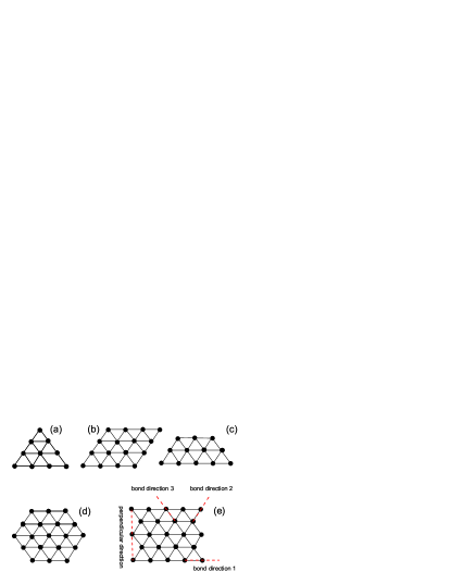
Figure 2: (a) The triangle-shaped triangular lattice with $N=4$. (b) The rhombus-shaped lattice with $N=4$. (c) The trapezoid-shaped lattice with $N=3$. (d) The hexagon-shaped lattice with $N=3$. (e) The rectangle-shaped lattice with $N=5$. Three bond directions and the perpendicular direction are shown (see text).

Table 5: The fitted edge, corner internal energy and $u_{k}$ for triangle and rectangle shape in Eq. (43). For triangle and rectangle shape, there is no other logarithmic corrections than surface and corner terms.

	triangle	rectangle
$u_{\rm surf}$	$-0.551328895421792049511325(9)$	$-0.5513288954217920495113(1)$
$u_{1}$	$~{}~{}~{}0.1358128850971729047321(2)$	$-1.124623054881823516433(4))$
$u_{\rm corn}$	$-1.65398668626537614853(3)$	$~{}~{}~{}0.1477281322922120845(6)$
$u_{2}$	$-1.4200975898148873036(2)$	$-1.236099923077146896(3)$
$u_{3}$	$-0.702623731123014999(6)$	$~{}~{}~{}0.3520087573021713(2)$
$u_{4}$	$-0.0272494452610576(5)$	$-0.04481963510134(2)$
$u_{5}$	$~{}~{}~{}0.01706870885164(4)$	$~{}~{}~{}0.141108181792(2)$
$u_{6}$	$-0.009549023082(3)$	$~{}~{}~{}0.0055256275(2)$
$u_{7}$	$~{}~{}~{}0.0102157015(1)$	$~{}~{}~{}0.10191756(1)$
$u_{8}$	$-0.009092781(5)$	$-0.2825362(7)$
$u_{9}$	$~{}~{}~{}0.0024505(1)$	$~{}~{}~{}0.40416(3)$
$u_{10}$	$~{}~{}~{}0.006205(2)$	$-0.7968(7)$
$u_{11}$	$-0.01636(3)$	$~{}~{}~{}0.04(1)$
$u_{12}$	$~{}~{}~{}0.0274(2)$	$~{}~{}~{}1.4(1)$
$u_{13}$	$-0.0232(6)$	$-7.9(6)$

For triangle and rectangle-shaped lattices, we fit the data with $k$ from $1$ to $13$. We find that there is no logarithmic correction in higher orders, i.e., $u_{lk}=0$. For rhombus, trapezoid and hexagon shape, we fit the data with $k$ from $1$ to $9$. We find that there are logarithmic corrections in higher orders. The higher order logarithmic corrections begins from $k=4$ as listed in Tab. 6.

The bulk value $U_{\infty}$ is known to be $2$ newell . Our fit of $U_{\infty}$ is $2.0+(3\pm 9)\times 10^{-23}$ for the hexagonal shape, which is the worst among five cases. The best one is $2.0\pm 10^{-25}$ for the triangle shape. From this one can see the accuracy of the BP algorithm reaches $10^{-25}$ at least.

The leading correction is due to the edges (or surfaces), which is unknown to our knowledge. We denote the surface internal energy per unit length of the edge along one bond direction by $u^{\parallel}_{\rm surf}$, and that perpendicular to that direction by $u^{\perp}_{\rm surf}$. For the triangular, rhomboid, trapezoid, and hexagonal shapes (see Table 5 and 6) , we have $u_{\rm surf}=u_{\rm surf}^{\parallel}$. For the rectangular shape we have $u_{\rm surf}=(2u_{\rm surf}^{\parallel}+\sqrt{3}u^{\perp}_{\rm surf})/(2+\sqrt{3})$, and

$$u_{\rm surf}^{\parallel} = -0.551328895421792049511325(9),$$

$$u_{\rm surf}^{\perp} = -0.5513288954217920495113(1).$$ (44)

This is an interesting result because it means that the surface internal energy per unit length is symmetric for an edge along or perpendicular to an arbitrary bond direction. We conjecture that the exact value of the surface internal energy is given by

$$u_{\rm surf}^{\parallel}=u_{\rm surf}^{\perp}=-\frac{\sqrt{3}}{\pi}=-0.551328895421792049511326\cdots$$ (45)

Table 6: The fitted edge, corner internal energy and $u_{k}$ for rhombus, trapezoid and hexagon shape in Eq. (43).

	rhombus	trapezoid	hexagon
$u_{\rm surf}$	$-0.55132889542179204946(7)$	$-0.551328895421792049501(7)$	$-0.5513288954217920497(5)$
$u_{1}$	$-0.728607166200085890(3)$	$-1.4553104976350188627(3)$	$-3.44983946582806485(3)$
$u_{\rm corn}$	$-0.7351051938957218(9)$	$-0.7351051938957225(1)$	$~{}~{}1.102657790843582(8)$
$u_{2}$	$-1.093360446288389(6)$	$-0.5538076013331216(8)$	$~{}~{}1.71029326576843(5)$
$u_{3}$	$-0.219739754536(1)$	$~{}~{}0.0257228180889(2)$	$-0.37845053923(2)$
$u_{4}$	$~{}~{}0.067693864(4)$	$-0.0117835146(8)$	$~{}~{}0.34795211(8)$
$u_{5}$	$-0.016510(1)$	$-0.0171482(3)$	$-0.28066(3)$
$u_{6}$	$~{}~{}0.0046(1)$	$~{}~{}0.09999(2)$	$~{}~{}0.271(4)$
$u_{7}$	$-0.113(3)$	$-0.2641(8)$	$-2.6(2)$
$u_{8}$	$~{}~{}0.14(1)$	$~{}~{}0.446(5)$	$-4(2)$
$u_{9}$	$-0.10(1)$	$-0.549(4)$	$-3.8(9)$
$u_{l4}$	$~{}~{}0.0335649470(7)$	$~{}~{}0.0420829435(1)$	$~{}~{}0.09678630(1)$
$u_{l5}$	$-0.0223773(2)$	$-0.04922954(5)$	$-0.055879(7)$
$u_{l6}$	$~{}~{}0.01797(3)$	$~{}~{}0.059675(7)$	$~{}~{}0.065(1)$
$u_{l7}$	$~{}~{}0.0104(9)$	$-0.0450(3)$	$~{}~{}0.55(6)$
$u_{l8}$	$~{}~{}0.012(9)$	$~{}~{}0.025(3)$	$~{}~{}5(1)$
$u_{l9}$	$~{}~{}0.06(1)$	$~{}~{}0.037(7)$	$~{}~{}15(3)$

Following the convention for the critical free energy, we write the coefficient of $(\ln N)/S$ as $u_{\rm corn}$. We denote the corner correction by $u_{\rm corn}^{(\gamma)}$, where $\gamma$ is the angle of the corner. Under the assumption that $u_{\rm corn}$ is the sum of the corner’s contributions, we have

$$u_{\rm corn}=\left\{\begin{array}[]{lcl}3u_{\rm corn}^{(\pi/3)}\hskip 62.59596pt\mbox{for triangle}\\ 2\left(u_{\rm corn}^{(\pi/3)}+u_{\rm corn}^{(2\pi/3)}\right)\hskip 5.69046pt\mbox{for rhombus and trapezoid}\\ 6u_{\rm corn}^{(2\pi/3)}\hskip 59.75095pt\mbox{for hexagon}\\ 4u_{\rm corn}^{(\pi/2)}\hskip 62.59596pt\mbox{for rectangle}\end{array}\right.$$

From the Tab. 5 and 6, we obtain the corner term for the three angles

$$u_{\rm corn}^{(\pi/3)} = -0.55132889542179204951(1)\approx-\frac{\sqrt{3}}{\pi},$$

$$u_{\rm corn}^{(\pi/2)} = 0.036932033073053021125(2),$$

$$u_{\rm corn}^{(2\pi/3)} = 0.1837762984739298(3)\approx\frac{1}{\sqrt{3}\pi}.$$ (47)

From this result, we can conjecture that the exact result of $u_{\rm corn}^{(\pi/3)}$ is $-\sqrt{3}/\pi$, $u_{\rm corn}^{(2\pi/3)}$ is $1/(\sqrt{3}\pi)$

There is no logarithmic corrections in higher order terms for the triangular and rectangular shapes. In contrast there are such terms for the rhombus, trapezoid and hexagon shapes. With the help of much more accurate data, we confirm the finding in the previous work wu2 that, for in critical free energy density, there is no logarithmic correction terms of order higher than $1/S$ for the triangular and rectangular shape, and there are such terms for the rhombus, trapezoid and hexagonal shape.

IV.2 Critical specific heat density

The data of the critical specific heat are fitted using the following formula

$$c = A^{\rm tri}_{0}\ln N+c_{0}+c_{\rm surf}\frac{p(N)\ln N}{S}+\frac{c_{1}}{S^{1/2}}$$ (48)

$$+\frac{c_{\rm corn}\ln N+c_{2}}{S}+\sum_{k=3}\frac{c_{k}+c_{lk}\ln N}{S^{k/2}},$$

where $p(N)$ is the perimeter. Compared with the expansion for the triangular lattice with periodic boundary conditions salas , there are additional logarithmic surface term and corner term.

Table 7: The fitted edge, corner internal specific heat and $c_{k}$ for triangle and rectangle shape in Eq. (48).

	triangle	rectangle
$A^{\rm tri}_{0}$	$~{}~{}0.499069378046460449833662(8)$	$~{}~{}0.4990693780464604498336723(9)$
$c_{0}$	$-0.80424240621924908720053(9)$	$-0.573388979085776611481176(9)$
$c_{\rm surf}$	$~{}~{}0.166356459348820149932(8)$	$~{}~{}0.138096991677687094105(1)$
$c_{1}$	$-0.1878730393246832268(2)$	$-0.08534785228081183795(4))$
$c_{\rm corn}$	$~{}~{}0.74860406706969065(1)$	$-0.150040848081735954(3)$
$c_{2}$	$~{}~{}0.64050897872895593(7)$	$~{}~{}0.68035027281155164(2)$
$c_{3}$	$~{}~{}0.341267433764613(2)$	$-0.0382477471847520(7)$
$c_{4}$	$~{}~{}0.0164170250248(1)$	$~{}~{}0.06815513150821(7)$
$c_{5}$	$-0.008335950854(7)$	$-0.027408848314(6)$
$c_{6}$	$~{}~{}0.0048860618(4)$	$~{}~{}0.0752274355(5)$
$c_{7}$	$-0.00632229(1)$	$-0.16560769(3)$
$c_{8}$	$~{}~{}0.0050319(4)$	$~{}~{}0.207074(1)$
$c_{9}$	$-0.002319(5)$	$-0.28531(5)$
$c_{10}$	$-0.032(2)$	$-0.112(1)$
$c_{11}$	$~{}~{}0.43(4)$	$~{}~{}0.85(2)$
$c_{12}$	$-2.8(3)$	$-3.6(2)$
$c_{13}$	$~{}~{}8(1)$	$~{}~{}3.3(9)$

For triangle and rectangle shape, we fit the data with $k$ from $1$ to $13$. We find that there is no logarithmic correction in higher order terms, i.e. $c_{lk}=0$. Therefore there is no $c_{lk}$ in Tab 7. For rhombus, trapezoid and hexagon shape, we fit the data with $k$ from $1$ to $9$. We find that there are logarithmic correction in higher order terms. The higher order logarithmic corrections begins from $k=3$ as shown in Tab. 8.

The leading term $A^{\rm tri}_{0}\ln N$ is known from the exact result salas , which reads

$$A^{\rm tri}_{0}=\frac{3\sqrt{3}}{4\pi}(\ln 3)^{2}=0.4990693780464604498336724\cdots.$$ (49)

Our fits, listed in Tab. 7 and 8, agree with the exact result at least in accuracy $10^{-21}$. The other fitted parameters are listed in Tab. 7 and 8 as well.

Table 8: The fitted edge, corner internal specific heat and $c_{k}$ for rhombus, trapezoid and hexagon shape in Eq. (48).

	rhombus	trapezoid	hexagon
$A^{\rm tri}_{0}$	$~{}~{}0.499069378046460449832(2)$	$~{}~{}0.4990693780464604498337(1)$	$~{}~{}0.499069378046460449831(1)$
$c_{0}$	$-0.60510340124288164836(2)$	$-0.519950222059951425774(2)$	$-0.26733979383373518196(1)$
$c_{\rm surf}$	$~{}~{}0.166356459348820142(8)$	$~{}~{}0.1663564593488201503(8)$	$~{}~{}0.166356459348820129(9)$
$c_{1}$	$-0.146850680614596(3)$	$-0.10404207253293299(4)$	$-0.2755298974420975(5)$
$c_{\rm corn}$	$~{}~{}0.3881650718138(1)$	$~{}~{}0.38816507181392(1)$	$-0.3327129186981(1)$
$c_{2}$	$-1.093360446288389(6)$	$~{}~{}0.6373742819503(8)$	$~{}~{}0.543662728665(1)$
$c_{3}$	$~{}~{}0.1409052856(8)$	$-0.023617749(8)$	$-0.0373484(1)$
$c_{4}$	$~{}~{}0.00563(3)$	$-0.0117835146(8)$	$~{}~{}0.34795211(8)$
$c_{5}$	$-0.016510()$	$~{}~{}0.027341(1)$	$~{}~{}0.03672(2)$
$c_{6}$	$~{}~{}-0.045(2)$	$-0.0232(1)$	$~{}~{}0.181(3)$
$c_{7}$	$-0.00(3)$	$~{}~{}0.084(3)$	$~{}~{}2.24(9)$
$c_{8}$	$~{}~{}0.2(1)$	$~{}~{}0.40(3)$	$~{}~{}16(1)$
$c_{9}$	$~{}~{}0.2(1)$	$~{}~{}0.95(5)$	$~{}~{}39(3)$
$c_{l3}$	$~{}~{}0.0269426979(1)$	$~{}~{}0.02995964044(2)$	$~{}~{}0.0787927005(2)$
$c_{l4}$	$-0.01404491(5)$	$~{}~{}0.00186976(4)$	$-0.0398024(6)$
$c_{l5}$	$~{}~{}0.011518(7)$	$~{}~{}0.011667(7)$	$~{}~{}0.0418(1)$
$c_{l6}$	$~{}~{}0.0009(4)$	$-0.0626(4)$	$-0.859(9)$
$c_{l7}$	$~{}~{}0.04(1)$	$~{}~{}0.021(8)$	$-3.1(3)$
$c_{l8}$	$~{}~{}0.15(8)$	$-0.82(4)$	$-21(2)$
$c_{l9}$	$~{}~{}0.1(1)$	$~{}~{}0.57(4)$	$~{}~{}11(1)$

The leading correction $p(N)\ln N/S$ is caused by the edges. We denote the surface specific heat per unit length of the edge along one bond direction by $c^{\parallel}_{\rm surf}$, and that perpendicular to the direction by $c^{\perp}_{\rm surf}$. For the triangle, rhombus, trapezoid, and hexagon shape, we have $c_{\rm surf}=c_{\rm surf}^{\parallel}$; for the rectangle, we set $c_{\rm surf}=(2c_{\rm surf}^{\parallel}+\sqrt{3}c^{\perp}_{\rm surf})/(2+\sqrt{3})$, and find

$$c_{\rm surf}^{\parallel} = 0.166356459348820149932(8)\approx\frac{A^{\rm tri}_{0}}{3},$$

$$c_{\rm surf}^{\perp} = 0.105465769143518701148(8).$$ (50)

Note that this term is absent in the torus case fisher1969 and not mentioned in the long strip case fisher , but exists in the cylinder case with Brascamp-Kunz boundary conditions Janke ; izmailian2002b . In addition, we conjecture that $c_{\rm surf}^{\parallel}=A^{\rm tri}_{0}/3$.

Following the convention for the critical free energy, we write the coefficient of $\ln N/S$ as $c_{\rm corn}$. We denote the corner correction by $c_{\rm corn}^{(\gamma)}$ where $\gamma$ is the angle of the corner. Again, under the assumption that the total correction is the sum of all corners, we have

$$c_{\rm corn}=\left\{\begin{array}[]{lcl}3c_{\rm corn}^{(\pi/3)}\hskip 62.59596pt\mbox{for triangle}\\ 2\left(c_{\rm corn}^{(\pi/3)}+c_{\rm corn}^{(2\pi/3)}\right)~{}~{}\mbox{for rhombus and trapezoid}\\ 6c_{\rm corn}^{(2\pi/3)}\hskip 59.75095pt\mbox{for hexagon}\\ 4c_{\rm corn}^{(\pi/2)}\hskip 62.59596pt\mbox{for rectangle}\end{array}\right.$$

From Tab. 7 and 8, we obtain the corner contribution of the three angles,

$$c_{\rm corn}^{(\pi/3)} = 0.249534689023230217(3)\approx\frac{A^{\rm tri}_{0}}{2},$$

$$c_{\rm corn}^{(\pi/2)} = -0.0375102120204339885(8),$$

$$c_{\rm corn}^{(2\pi/3)} = -0.05545215311627(5)\approx\frac{A^{\rm tri}_{0}}{9}.$$ (52)

We conjecture that $c_{\rm corn}^{(\pi/3)}=A^{\rm tri}_{0}/2$ and $c_{\rm corn}^{(2\pi/3)}=A^{\rm tri}_{0}/9$.

In the previous section on the square lattice, we obtained the corner term $c_{\rm corn}=0.3709039421492394(2)$ for the rectangular shape with various aspect ratios. It is different from the present result $-0.150040848081735954(3)$ for the rectangle-shaped triangular lattice. This indicates that the corner term of the specific heat depends on the microscopic structure of the lattice, thus is not universal.

V Summary and discussion

We have developed the BP algorithm for the specific heat and made the BP algorithm for the internal energy completed. With these algorithm, we have studied the surface and corner quantities via a numerically exact approach on 2D lattices with free boundaries, which permits us to extract very precisely many terms in their asymptotic expansions, and sometimes even allows conjectures of their exact values. This work is a continuation of earlier works wu ; wu2 by the three of the present authors, but here addressing specifically the internal energy and the specific heat. There are two remarkable progresses comparing with previous work wu ; wu2 :

I. Some exact edge and corner terms are conjectured from the accurate numerical fits. For the rectangular shape on the square lattice, the exact edge term and corner term of internal energy and specific heat $u_{\rm surf},u_{\rm corner},c_{\rm surf},c_{\rm corn}$ are conjectured. From the results for various shapes on the triangular lattice, we conjectured the exact edge and corner terms $u_{\rm surf}^{\parallel}$, $u_{\rm surf}^{\perp}$,$u_{\rm corn}^{(\pi/3)}$, $u_{\rm corn}^{(2\pi/3)}$, $c_{\rm surf}^{\parallel}$,$c_{\rm corn}^{(\pi/3)}$, $c_{\rm corn}^{(2\pi/3)}$. These conjectured exact results imply that there should exist closed form analytical solutions for these cases with free boundaries.

II. The accurate forms of finite-size scaling for the internal energy and specific heat are determined. For the rectangular shape on the square and triangular lattice, there is no logarithmic correction terms of order higher than $1/S$. For the triangle shape on the triangular lattice, there is also no logarithmic correction terms higher that $1/S$. For the rhombus, trapezoid and hexagonal shape on the triangular lattice, there exist logarithmic correction terms of order higher than $1/S$ for the internal energy, and logarithmic correction terms of all orders for the specific heat. This property seems harmonic. The origin of these higher order logarithmic corrections are an interesting topic for the RG and CFT.

With Vernier and Jacobsen’s analytical solution jacobsen , one can study the internal energy and specific heat. However this calculation has not been carried out. It should be interesting to compare the results obtained by their solution and our numerical results with the BP algorithm.

acknowledgment This work is supported by the National Science Foundation of China (NSFC) under Grant No. 11175018. N.I. is also supported by FP7 EU IRSES Project No. 295302 (Statistical Physics in Diverse Realizations) and by a Marie Curie International Incoming Fellowship within the 7th European Community Framework Programme.

References

• (1) V. Privman and M. E. Fisher, Phys. Rev. B 30, 322 (1984).
• (2) V. Privman, Phys. Rev. B 38, 9261 (1988).
• (3) H. W. J. Blöte, J. L. Cardy, and M. P. Nightingale, Phys. Rev. Lett. 56, 742 (1986).
• (4) J. L. Cardy and I. Peschel, Nucl. Phys. B 300, 377 (1988).
• (5) L. Onsager, Phys. Rev. 65, 117 (1944).
• (6) B. Kaufman, Phys. Rev. 76, 1232 (1949).
• (7) G. F. Newell, Phys. Rev. 79, 876 (1950); R. M. F. Houttapel, Physica 16, 425 (1950).
• (8) A. E. Ferdinand and M. E. Fisher, Phys. Rev. 185, 832 (1969)
• (9) H. Au-Yang and M. E. Fisher, Phys. Rev. B 11, 3469 (1975).
• (10) E. V. Ivashkevich, N. Sh. Izmailian and C.-K. Hu, J. Phys. A 35 (2002) 5543.
• (11) J. Salas, J. Phys. A: Math. Gen. 35 1833 (2002).
• (12) N. Sh. Izmailian and C.-K. Hu, Phys. Rev. E. 76, 041118 (2007).
• (13) N. Sh. Izmailian, K. B. Oganesyan and C.-K. Hu, Phys. Rev. E 65 (2002) 056132.
• (14) W. Janke and R. Kenna, Phys. Rev. B 65, 064110 (2002).
• (15) N. Sh. Izmailian and C.-K. Hu, Phys. Rev. Letts. 86, 5160 (2001).
• (16) D. P. Landau, Phys. Rev. B 13, 2997 (1976).
• (17) B. Stošić, S. Milošević and H. E. Stanley, Phys. Rev. B , 41, 11466 (1990).
• (18) P. Kleban and I. Vassileva, J. Phys. A: Math. & Gen. 24, 3407 (1991).
• (19) R. Bondesan, J. Dubail, J. L. Jacobsen, H. Saleur, Nucl. Phys. B 862[FS], 553 (2012).
• (20) Y. Imamura, H. Isono, and Y. Matsuo, Prog. Theor. Phys., 115, 979 (2006).
• (21) M.R. Gaberdiel and I. Runkel, J. Phys. A: Math. Theor. 41 075402 (2008).
• (22) N. Read and H. Saleur, Nucl. Phys. B 777, 316 (2007).
• (23) I. Affleck, in: Lecture Notes, Les Houches Summer School, vol. 89, July 2008, Oxford University Press, 2010, arXiv:0809.3474.
• (24) I. Affleck and A.W.W. Ludwig, J. Phys. A: Math. Gen. 27 5375 (1994).
• (25) P. Calabrese and J. Cardy, J. Stat. Mech. P10004 (2007).
• (26) J. Dubail and J.-M. Stéphan, J. Stat. Mech. L03002 (2011); J.-M. Stéphan and J. Dubail, J. Stat. Mech. P08019 (2011).
• (27) M. Bauer and D. Bernard, Phys. Rep. 432, 115 (2006).
• (28) E. Vernier and J. L. Jacobsen, J. Phys. A: Math. Gen. 45, 045003 (2012).
• (29) Y. L. Loh and E.W. Carlson, Phys. Rev. Lett. 97, 227205 (2006).
• (30) Y. L. Loh, E.W. Carlson, and M. Y. J. Tan, Phys. Rev. B 76, 014404 (2007).
• (31) M. Caselle, M. Hasenbusch, A. Pelissetto and E. Vicari, J. Phys. A: Math. Gen. 35, 4861 (2002).
• (32) S. L. A. de Queiroz, Phys. Rev. E 84, 031107 (2011).
• (33) X.-T. Wu, N. Sh. Izmailian, and W.-A. Guo, Phys. Rev. E 86, 041149 (2012).
• (34) X.-T. Wu, N. Sh. Izmailian, and W.-A. Guo, Phys. Rev. E 87, 022124 (2013).