A Predicted New Population of UV-faint Galaxies at $z\ga 4$

Abstract

We show that a bursty model of high redshift star formation explains several puzzling observations of the high redshift galaxy population. We begin by pointing out that the observed specific star formation rate requires a duty-cycle of $\sim 10\%$, which is much lower than found in many hydro-dynamical simulations. This value follows directly from the fact that the observed star formation rate in galaxies integrated over a Hubble time exceeds the observed stellar mass by an order of magnitude. We use the large observed specific star formation rate to calibrate the efficiency of feedback in a model for the high redshift star formation rate which includes merger driven star formation regulated by SNe feedback. This model reproduces the star formation rate density function and the stellar mass function of galaxies at $4\la z\la 7$. A prediction of the model is that the specific star formation rate does not evolve very rapidly with either mass or redshift, in agreement with observation. This is in contrast to results from hydrodynamical simulations where the star formation closely follows the accretion rate, and so increases strongly towards high redshift. The bursty star formation model naturally explains the observation that there is not enough stellar mass at $z\sim 2-4$ to account for all of the star-formation observed, without invoking properties like an evolving initial mass function of stars. The finding of a duty cycle that is $\sim 10\%$ implies that there should be ten times the number of known galaxies at fixed stellar mass that have not yet been detected through standard UV selection at high redshift. We therefore predict the existence of a large undetected population of UV-faint galaxies that accounts for most of the stellar mass density at $z\sim 4-8$.

1 Introduction

The galaxy luminosity function is the primary observable that must be reproduced by any successful model of galaxy formation. At $z~{}\hbox to0.0pt{$>$\hss}{\lower 4.30554pt\hbox{$\sim$}}6$, it also represents one of the most important observables for studying the reionization of cosmic hydrogen. The luminosity function of Lyman-break galaxy (LBG) candidates discovered at $z\ga 6$ in recent WFC3/IR surveys is described by a Schechter function with characteristic density $\Psi_{\star}$ in comoving Mpc^-3, and a power-law slope $\alpha$ at luminosities $L$ below a characteristic break $L_{\star}$ (e.g. Bouwens et al., 2011; Oesch et al., 2012; Loeb & Furlanetto, 2012; McLure et al., 2012; Ellis et al., 2013; Oesch et al., 2013). Developing a theoretical picture of the important processes involved in setting the star formation rate at high redshift lies at the forefront of understanding this important cosmic epoch (e.g. Trenti et al., 2010; Finlator et al., 2011; Muñoz & Loeb, 2011; Raičević et al., 2011; Salvaterra et al., 2011).

Complex hydrodynamical models have been used to model the observed properties of high redshift galaxies. For example Finlator et al. (2011) have modelled the growth of stellar mass in high redshift galaxies using hydrodynamical simulations coupled with sub-grid models for processes including star formation and metal enrichment, and broadly reproduce the luminosity function evolution as well as the blue colours of the young stellar populations at high redshift. Similarly, Salvaterra et al. (2011) and Jaacks et al. (2012) have calculated the evolution of the luminosity function in detailed numerical simulations including calculations of enrichment and dust reddening, with the latter also including additional physics related to the transition from population-III to population-II stars. While these models are able to reproduce the luminosity function and star formation rate density function, they over-produce the high redshift stellar mass function, particularly at the low mass end.

Recently, Wyithe & Loeb (2013) presented a model for the high redshift star formation rate density function, which includes merger driven star formation regulated by SNe feedback. This model fits a range of observables, and implies a duty cycle of star formation of only 1-10%, much lower than found in hydro-dynamical simulations. The model successfully predicts the observed relation between star formation rate and stellar mass at $z~{}\hbox to0.0pt{$>$\hss}{\lower 4.30554pt\hbox{$\sim$}}4$. Supernovae feedback was found to lower the efficiency of star formation in the lowest mass galaxies, making their contribution to reionization small.

A puzzling observation in recent high redshift galaxy research has been that the star formation rate per stellar mass (specific star formation rate; sSFR) does not seem to evolve significantly with either mass or redshift (e.g. Stark et al., 2009; González et al., 2010). While subsequent analyses indicated that the absolute value of the sSFR at $z\geq 4$ might have been underestimated in these first derivations after including updated estimates of dust extinction and accounting for the impact of rest-frame optical emission lines, the current best observational estimates indicate only slow evolution across $z\sim 4-7$ (see e.g. Gonzalez et al., 2012; Stark et al., 2013). However, the observational debate is far from settled (e.g. Smit et al., 2013).

Most simulations of high redshift galaxy formation do not reproduce the observed plateauing of specific star formation rate at $z>2$. This is because simulations generally associate star formation primarily with the accretion of gas. As a result they predict a rapid increase in the specific star formations rate, which can be understood because the specific accretion rate is found to scale as $(1+z)^{2.5}$ (Neistein & Dekel, 2008). To understand which aspect of high redshift galaxy formation models drives the incorrect prediction of an evolving specific star formation rate, Weinmann et al. (2011) calculated the specific star formation history within a suite of semi-analytic models. At $z>4$, they found that the evolution of specific star formation rate could be reproduced in the presence of strong SNe feedback. In this paper, we find that a SNe regulated model with star-formation triggered by mergers and a low duty cycle naturally reproduces both the large value of specific SFR, and the observed behaviour with mass and redshift.

The relationship between the observed star formation rate and stellar mass per unit volume has also been an observational focus. Wilkins et al. (2008) compiled estimates of stellar mass and star formation rates as a function of redshift in order to investigate whether the integral of star formation rate matches the observed stellar mass. Puzzlingly, at $z\sim 2-4$, Wilkins et al. (2008) find that there is not enough stellar mass to account for all of the star-formation observed. Conversely, at high redshift Bouwens et al. (2011) and Robertson et al. (2013) find that the observed stellar mass is accounted for by the observed star-formation rate (see also Stark et al., 2013). In this paper we argue that both observations can be understood in the context of a star formation model with a duty-cycle of order 10%.

We begin in § 2 by pointing out the general constraint on the duty-cycle that is provided by observations of the specific star formation rate. Then, in § 3 we briefly summarise the model for high redshift star formation presented in Wyithe & Loeb (2013). We next present a comparison of this model with various observables including the star formation rate density function, specific star formation rate, clustering amplitude and stellar mass function in § 4. We discuss the detectability of a predicted population of low UV luminosity galaxies in § 5, and finish with a discussion in § 6. In our numerical examples, we adopt the standard set of cosmological parameters (Komatsu et al., 2011), with values of $\Omega_{\rm b}=0.04$, $\Omega_{\rm m}=0.24$ and $\Omega_{\Lambda}=0.76$ for the density parameters of matter, baryon, and dark energy, respectively, $h=0.73$, for the dimensionless Hubble constant, and $\sigma_{8}=0.82$.

2 The specific star formation rate of star-forming galaxies

Before discussing our particular model for supernovae (SNe) regulated star formation, we begin by looking at the very general constraint on duty-cycle ($\epsilon_{\rm duty,tot}$) provided by the specific star formation rate. In the simplest model of constantly star-forming galaxies, the specific star formation rate is

$$sSFR=\frac{SFR}{M_{\star}}=\frac{SFR}{SFR\times(\epsilon_{\rm duty,tot}H^{-1})}=(\epsilon_{\rm duty,tot}H^{-1})^{-1}.$$ (1)

Thus, the specific star formation rate leads to a direct estimate of the duty cycle of star formation averaged over a Hubble time. This is plotted in the upper two panels of Figure 1 as a function of redshift for $\epsilon_{\rm duty,tot}=0.1$ and 0.15 (solid lines), compared with observations of specific star formation rate at stellar masses of $M_{\star}=10^{9}$M_⊙ and $M_{\star}=5\times 10^{9}$M_⊙ respectively. The dotted lines also show the curves corresponding to a duty-cycle of unity, illustrating the level at which the values of specific star formation rate deviate from expectations of continuous star formation. We note the weak dependence of the inferred duty-cycle over the range of stellar mass and redshift probed. This low duty cycle has a range of important implications for the properties of the high redshift galaxy population, and explains several puzzling properties of the observed relation between stellar mass and star formation rate. For the remainder of this paper we explore these explanations in the context of the merger driven model of Wyithe & Loeb (2013). However we stress that the result of low duty-cycle from equation (1) is very general and not dependent on the details of our particular star formation model.

3 Model

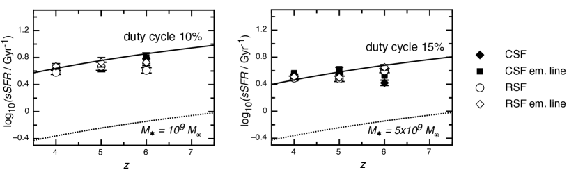
Figure 1: The specific star-formation rate as a function of redshift calculated based on equation (1) for duty-cycles of 10% and 15% (solid lines) and 100% (dotted lines), in comparison with measurements at stellar masses of $10^{9}$ and $5\times 10^{9}$ M_⊙. The data points are from Gonzalez et al. (2012), and the labels represent stellar masses based on the assumptions of a constant (CSF) and rising (RSF) star-formation history without and with emission lines included (em. line) as described in that paper.

A complication that arises when modelling the luminosity function is that models predict a star formation rate, which must then be converted to an observed luminosity assuming a dust extinction and an initial mass function (IMF) for the stars. A better comparison between theory and observations is therefore to estimate the star formation rate density observationally, where the correction is made from luminosity to star formation rate using the observed continuum properties of the galaxies under study. Following the approach of Wyithe & Loeb (2013) we therefore focus on modelling the SFRD function (Smit et al., 2012) rather than the luminosity function of high redshift galaxies.

In this section we briefly summarise the model for star formation in high redshift galaxies presented in Wyithe & Loeb (2013). The reader is referred to that paper for further details of this model. The star formation rate in a galaxy halo of mass $M$ that turns a fraction $f_{\star}$ of its disk mass $m_{d}M$ into stars over a time $t_{\rm SF}$ is

$$SFR=0.15\mbox{M}_{\odot}\mbox{yr}^{-1}\left(\frac{m_{\rm d}}{0.17}\right)\left(\frac{f_{\star}}{0.1}\right)\left(\frac{M}{10^{8}\mbox{M}_{\odot}}\right)\left(\frac{t_{\rm SF}}{10^{7}\mbox{yr}}\right)^{-1}.$$ (2)

The model assumes that major mergers trigger bursts of star formation. The star formation rate density function (i.e. galaxies per Mpc³ per unit of $SFR$) can be estimated as

$$\Phi(SFR)=$$

$$\epsilon_{\rm duty}\left(\Delta M\left.t_{\rm H}\frac{dN^{2}_{\rm merge}}{dtd\Delta M}\right|_{M_{1},\Delta M}\frac{dn}{dM}\right)\left(\frac{dSFR}{dM}\right)^{-1},$$ (3)

where $\epsilon_{\rm duty}$ is the fraction of the Hubble time ($t_{\rm H}$) over which each burst lasts, and $dn/dM$ is mass function of dark matter halos (Press & Schechter, 1974; Sheth & Tormen, 1999). The rate of major mergers ($dN_{\rm merge}/dt$) is calculated as the number of halos per logarithm of mass $\Delta M$ per unit time that merge with a halo of mass $M_{1}$ to form a halo of mass $M$ (Lacey & Cole, 1993). We assign a 2:1 mass ratio to major mergers (i.e. $M_{1}=\frac{2}{3}M$ and $\Delta M=M/3$).

The most massive stars fade away on a timescale of $t_{\rm s}\sim 3\times 10^{6}$ years (Barkana & Loeb, 2001). If the starburst lifetime is $t_{\rm SF}$ the duty-cycle can be written as

$$\epsilon_{\rm duty}=\frac{t_{\rm s}+t_{\rm SF}}{t_{\rm H}}.$$ (4)

For comparison with observations we define

$$\Psi(SFR)=\ln{10}\times SFR\times\Phi,$$ (5)

which has units of Mpc^-3 per dex.

We expect that SNe feedback will alter the fraction of gas in a galaxy that is turned into stars (e.g. Dekel & Woo, 2003). To determine the mass and redshift dependence of $f_{\star}$ in the presence of SNe we suppose that stars form with an efficiency $f_{\star}$ out of the gas that collapses and cools within a dark matter halo and that a fraction $F_{\rm SN}$ of each supernova energy output, $E_{\rm SN}$, heats the galactic gas mechanically (allowing for some losses due to cooling). The mechanical feedback will halt the star formation once the cumulative energy returned to the gas by supernovae equals the total thermal energy of gas at the virial velocity of the halo (e.g. Wyithe & Loeb, 2003). Hence, the limiting stellar mass is set by the condition

$$\frac{M_{\star}}{w_{\rm SN}}E_{\rm SN}F_{\rm SN}f_{\rm t}f_{\rm d}=E_{\rm b}=\frac{1}{2}m_{\rm d}Mv_{\rm vir}^{2}.$$ (6)

In this relation $E_{\rm b}$ is the binding energy in the halo, $w_{\rm SN}$ is the mass in stars per supernova explosion, and the total stellar mass is $M_{\star}=m_{\rm d}\,M\,f_{\rm\star,tot}$ where $f_{\rm\star,tot}=N_{\rm merge}f_{\star}$ is the total fraction of the gas that is converted to stars during major mergers, and $N_{\rm merge}$ is the number of major mergers per Hubble time. The parameters $f_{\rm t}$ and $f_{\rm d}$ denote the fraction of the SNe energy that contributes because of the finite timescale of the SNe feedback or the disk scale height being smaller than the SNe bubble. These terms are described in more detail below.

The ratio between the total mass in stars and dark matter is observed to increase with halo mass as $(M_{\star}/M)\propto M^{0.5}$ for $M_{\star}\la 3\times 10^{10}$M_⊙, but is constant for larger stellar masses (Kauffmann et al., 2003). Thus, the star formation efficiency within dwarf galaxies decreases towards low masses. For comparison with equation (6), a Scalo (1998) mass function of stars has $w_{\rm SN}\sim 126$ M_⊙ per supernova and $E_{\rm SN}=10^{51}$ ergs, and so we find that $M_{\star}=3\times 10^{10}$ M_⊙ and $v_{\rm c}\sim 175$ km/s (the typical value observed locally; see e.g. Bell & de Jong, 2001) implies $f_{\rm\star,tot}\sim 0.1$ for a value of $F_{\rm SN}\sim 0.5$. Smaller galaxies have smaller values of $f_{\star}$. Equation (6) indicates that

$$f_{\star}=$$

$$\min\left[f_{\rm\star,max},\frac{0.008}{N_{\rm merge}}\left(\frac{M}{10^{10}\mbox{M}_{\odot}}\right)^{\frac{2}{3}}\left(\frac{1+z}{10}\right)\left(f_{\rm t}f_{\rm d}F_{\rm SN}\right)^{-1}\right].$$ (7)

We utilise equation (3) with equation (3) as a function of the parameters $t_{\rm SF}$ and $f_{\rm\star,max}$.

3.1 Disk structure

The effect of SNe feedback is dependent on the conditions of the interstellar medium (ISM) gas. We assume that the cold gas (out of which stars form) occupies a self-gravitating exponential disk where $R_{\rm d}$ is the scale radius, $m_{\rm d}$ is the mass fraction of the disk relative to the halo and $\lambda\sim 0.05$ is the spin parameter of the halo (Mo et al., 1998). The scale height of the disk at radius $r$ is

$$H=\frac{c_{\rm s}^{2}}{\pi G\Sigma(r)},$$ (8)

where $c_{\rm s}$ is the sound speed in the gas, which we assume to have a temperature of $10^{4}$K, and $\Sigma(r)$ is the surface density. We adopt the density in the mid plane at the scale radius, within which half the gas is contained, as representative of the density of the ISM.

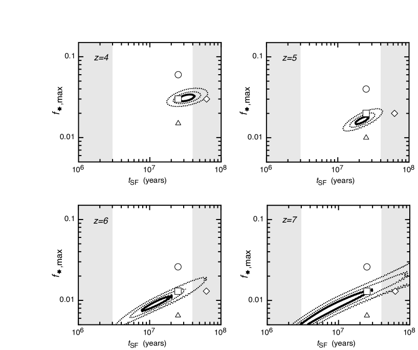
Figure 2: Constraints on the model parameters $f_{\rm\star,max}$ and $t_{\rm SF}$ at four different redshifts (constraints are independent at each redshift). In each case, three contours are shown corresponding to differences in $\chi^{2}$ relative to the best-fitting model of $\Delta\chi^{2}=\chi^{2}-\chi^{2}_{\rm min}=1$, 2.71 and 6.63. Projections of these contours on to the axes provide the 68.3, 90 and 99 per cent confidence intervals on individual parameter values. The vertical grey regions represent time-scales longer/shorter than the lifetime of the highest/lowest mass SNe progenitor ($3\times 10^{6}$yr$/4\times 10^{7}$yr).

3.2 Supernova evacuation of the ISM

Clarke & Oey (2002) presented a simple analytic model for the effect of supernovae on the interstellar medium which we apply to high redshift galaxies. In this model, clusters of $N_{\rm e}$ SNe produce super-bubbles in the ISM with a radius $R_{\rm e}$ at which the super-bubble comes into pressure balance with the ISM. This radius can be found by approximating $R_{\rm e}$ as the radius within which the thermal energy of the ISM equals the mechanical energy of the SNe cluster. The timescale associated with the evacuation of a super bubble in the ISM by a SNe cluster is $t_{\rm e}=4\times 10^{7}$ years, corresponding to the lifetime of the lowest mass SNe progenitor. The evacuation radius for a cluster of $N_{\rm e}$ SNe, each with energy output $E_{\rm SN}$ within an ISM of sound speed $c_{\rm s}$ is

$$R_{e} = 0.08\,\mbox{kpc}\left(\frac{N_{\rm e}}{10}\right)^{\frac{1}{3}}\left(\frac{E_{\rm SN}}{10^{51}\mbox{erg}}\right)^{\frac{1}{3}}\left(\frac{\lambda}{0.05}\right)^{\frac{4}{3}}\left(\frac{m_{\rm d}}{0.17}\right)^{-\frac{2}{3}}$$ (9)

$$\hskip 14.22636pt\times\left(\frac{M}{10^{8}\mbox{M}_{\odot}}\right)^{-\frac{2}{9}}\left(\frac{1+z}{10}\right)^{-\frac{4}{3}}.$$

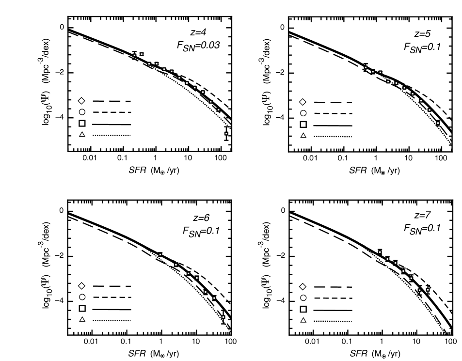
Figure 3: Comparison between the observed and modelled SFRD function (plotted as $\Psi=\ln{10}\times SFR\times\Phi$). The four panels show results for different redshift values. The observed SFRD functions from Smit et al. (2012) are shown as small open squares. In each panel, the four curves correspond to a different choice of model parameters $t_{\rm SF}$ and $f_{\rm\star,max}$, labelled by the symbols in Figure 2. The thick solid lines represent values close to the best fit.

In the limit where SNe evacuated regions are smaller than the scale height of the disk, and the starburst lifetime $t_{\rm SF}$ is much larger than the gas evacuation timescale $t_{\rm e}$, the fraction $F_{\rm SN}$ of the SNe energy may be used in feedback suppressing subsequent star formation. However, if the SNe evacuated regions break out of the disk, or $t_{\rm SF}<t_{\rm e}$, not all of the energy will be available for feedback. Based on the ISM porosity model of Clarke & Oey (2002), a fraction $f_{\rm d}=2H/R_{\rm e}$ of the SNe energy goes to increasing the ISM porosity for disks where $R_{\rm e}>H$. In this case we find

$$f_{\rm d} = 0.85\left(\frac{N_{\rm e}}{10}\right)^{-\frac{1}{3}}\left(\frac{E_{\rm SN}}{10^{51}\mbox{erg}}\right)^{-\frac{1}{3}}\left(\frac{\lambda}{0.05}\right)^{\frac{2}{3}}\left(\frac{m_{\rm d}}{0.17}\right)^{-\frac{1}{3}}$$ (10)

$$\times \hskip 14.22636pt\left(\frac{M}{10^{8}\mbox{M}_{\odot}}\right)^{-\frac{1}{9}}\left(\frac{1+z}{10}\right)^{-\frac{2}{3}}\left(\frac{c_{\rm s}}{10\mbox{km/s}}\right)^{2},$$

as long as $f_{\rm d}<1$ and $f_{\rm d}=1$ otherwise. Similarly, in cases where $t_{\rm SF}<t_{\rm e}\sim 4\times 10^{7}$ yrs, only

$$f_{\rm t}\equiv(t_{\rm SF}/t_{\rm e})^{2}$$ (11)

of the overall SNe energy output is generated by the time the starburst concludes. The quadratic dependence on time arises because the number of bubbles produced grows in proportion to time, while the maximum size of a bubble at time $t<t_{\rm e}$ is also proportional to time (Oey & Clarke, 1997). In cases where $t_{\rm SF}>t_{\rm e}$ we have $f_{\rm t}=1$.

4 Results

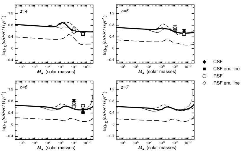
Figure 4: The specific star-formation rate for the models in Figure 3 as a function of stellar mass (as predicted by the star-burst only model). The data points are from Gonzalez et al. (2012), and the labels represent stellar masses based on the assumptions of a constant (CSF) and rising (RSF) star-formation history without and with emission lines included (em. line) as described in that paper.

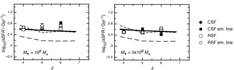
Figure 5: The specific star-formation rate for the models in Figure 3 as a function of redshift at stellar masses of $10^{9}$M_⊙ and $5\times 10^{9}$M_⊙. The data points are from Gonzalez et al. (2012), and the labels represent stellar masses based on the assumptions of a constant (CSF) and rising (RSF) star-formation history without and with emission lines included (em. line) as described in that paper.

Wyithe & Loeb (2013) used the merger driven model described above to argue that the duty cycle for star formation in high redshift galaxies was a few percent. However, while much lower than unity the model independent estimate based on the specific star formation rate shown in Figure 1 is significantly larger, with a value of $\sim 0.1$. To understand the origin of this difference we note that there is a degeneracy in the model between the duty-cycle $\epsilon_{\rm duty}$ and the parameter $F_{\rm SN}$ which governs the fraction of SNe energy that is harnessed for feedback. Wyithe & Loeb (2013) arbitrarily chose a value for this parameter since it is unconstrained by just the SFR density function. However, for the analysis in this paper the inclusion of the constraint on specific star formation rate allows us to constrain the value of $F_{\rm SN}$ in addition to the values of $f_{\rm\star,max}$ and $t_{\rm SF}$.

4.1 Comparison with observations

We fit our model to the recent determination of the SFRD function from Smit et al. (2012), and the specific star formation rate from Gonzalez et al. (2012) in order to constrain the three free parameters of our star formation model $t_{\rm SF}$ and $f_{\star}$. We fit separately for four different redshifts $z\sim 4$, 5, 6 and 7. Specifically we use the model to calculate SFRD functions and sSFR for combinations of these parameters and calculate the $\chi^{2}$ of the model as

$$\chi^{2}(f_{\rm\star,max},t_{\rm SF}) =$$ (12)

$$\sum_{i=0}^{N_{\rm obs}}\left(\frac{\log{\Psi(SFR_{i},f_{\rm\star,max},t_{\rm SF},z)}-\log{\Psi_{\rm obs}(SFR_{i},z)}}{\sigma_{SFR}(SFR_{i},z)}\right)^{2}$$

$$+\left(\frac{\log{sSFR(f_{\rm\star,max},t_{\rm SF},z)}-\log{sSFR_{\rm obs}(z)}}{\sigma_{sSFR}(z)}\right)^{2}$$

Here $\Psi_{\rm obs}(SFR_{i},f_{\rm\star,max},t_{\rm SF},z)$ is the observed star formation rate density measured at redshift $z$, with uncertainty in dex of $\sigma_{SFR}(SFR_{i})$. In calculating likelihoods at $z\sim 4$ and $z\sim 5$ we increased the quoted error bars by factors of 3 and 2 respectively in order to obtain a reduced $\chi^{2}$ of order unity. The value of sSFR is evaluated at a stellar mass of $M_{\star}=10^{9}$M_⊙, with uncertainties corresponding to the range of estimates for the two assumed star formation histories and the two cases of with/without emission lines considered in Gonzalez et al. (2012). The SFRD function and sSFR are sensitive to the value of $F_{\rm SN}$, and we therefore integrate the likelihood over a range of values uniformly distributed between $-2.5<\log_{10}{F_{\rm SN}}<0$

$$\mathcal{L}(f_{\rm\star,max},t_{\rm SF})\propto\int_{-1}^{0}d(\log_{\rm 10}{F_{\rm SN}})e^{-\chi^{2}/2}.$$ (13)

We note that the relation between $SFR$ and $M$ in equation (2) is not perfect. As part of our comparison with observations, and to account for scatter in this relationship, we convolve the predicted SFRD function from equation (3) with a Gaussian of width $0.5$ dex in $SFR$. An intrinsic scatter of 0.5 dex is motivated by the scatter in stellar mass at constant $SFR$ found by González et al. (2011). However, in addition we find that the value of 0.5 dex provides the best statistical fit to the observations. Our qualitative results are not sensitive to the choice of this scatter.

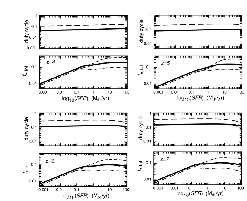
Figure 6: The values of total star formation efficiency $f_{\rm\star,tot}$ (i.e. the sum of $f_{\rm\star}$ over all mergers), and the overall duty-cycle (i.e. the fraction of a Hubble time during which a galaxy is star bursting) as a function of $SFR$. The four curves shown correspond to the SFRD functions shown in Figure 3, with model parameters $t_{\rm SF}$ and $f_{\rm\star,max}$ designated by the symbols in Figure 2.

4.2 Parameter constraints

In Figure 2 we show constraints on models. Given these sSFR driven constraints on $F_{\rm SN}$, we find that the shape of the SFRD function requires starburst durations of a few tens of Myr at $z\sim 5$, $z\sim 6$ and $z\sim 7$, with a few percent of the gas turned into stars per burst. For comparison the left and right hand vertical grey regions represent times smaller than the lifetime of the most massive stars ($t_{\rm s}\sim 3\times 10^{6}$ years), and times in excess of the lifetime of the least massive stars that produce SNe respectively. Our results therefore indicate that star formation in high redshift galaxies is terminated on the same timescale as feedback from SNe can be produced (Wyithe & Loeb, 2013).

Figure 3 shows the comparison between observed and modelled SFRD functions for four different redshifts $z\sim 4$, 5, 6 and 7 with values of $F_{\rm SN}=0.03$ at $z=4$ and $F_{\rm SN}=0.1$ at $z=5,6$ and 7 (c.f. $F_{\rm SN}=0.1$ and 0.3 in Wyithe & Loeb (2013)). The burst lifetime is $t_{\rm SF}=2.5\times 10^{7}$ years in each case. The four curves shown correspond to model parameters $t_{\rm SF}$ and $f_{\rm\star,max}$ labeled by the symbols in Figure 2. The thick solid lines show models close to the best fit to the observational data. The other three values were chosen so as to illustrate the dependence of the predicted SFRD function on the different parameters.

4.3 Specific star formation rate

Figure 4 shows the specific star formation rate as a function of mass for the models listed in Figure 3 at $z=4$, 5, 6 and 7, illustrating the success of the model in reproducing the observed specific star formation rate for the constrained parameters (particularly $F_{\rm SN}$). Beyond the narrow range of observed stellar mass values, the model predicts that the specific star-formation rate remains quite insensitive to stellar mass (or star formation rate). In this figure the wiggles result from the simple assumption of an abrupt change in efficiency with halo mass in equation (3). Figure 5 shows the specific star formation rate as a function of redshift for these models, illustrating the model prediction that the specific star-formation rate does not evolve with redshift. This finding is in agreement with observations, but in contrast to results from many hydrodynamical models of galaxy formation, indicating that star formation activity does not directly follow the gas accretion rate.

4.4 Star formation efficiency and average duty-cycle

The parameters $f_{\rm\star,max}$ and $t_{\rm SF}$ refer to single bursts, whereas our model includes multiple bursts occurring at the rate of major mergers. We therefore calculate the total star formation efficiency $f_{\rm\star,tot}=H^{-1}\,dN_{\rm merge}/dt\,f_{\star}$ (i.e. the sum of $f_{\rm\star}$ over all mergers during a Hubble time), as well as the overall duty-cycle $\epsilon_{\rm duty,tot}=N_{\rm merge}t_{\rm SF}/t_{\rm H}=t_{\rm SF}\,dN_{\rm merge}/dt$. These quantities are plotted in Figure 6 based on our model with parameter choices corresponding to the examples in Figure 3. We find that $\sim 5-10\%$ of the gas forms stars in bright galaxies of $SFR\sim 1-100$M_⊙ per year, with lower fractions down to a percent in fainter galaxies. This trend is in qualitative agreement with the observations of Lee et al. (2012) to explain the stellar mass vs UV luminosity relation. We find duty-cycles of $\sim 10-20$%, with higher duty-cycles at higher redshift reflecting the increased ratio between the lifetime of massive stars and the age of the Universe. The duty cycle is also larger for systems of higher star formation rate. This trend is in agreement with the observational estimate of Lee et al. (2009) based on a comparison of the luminosity and clustering of luminous $z\ga 4$ galaxies. These authors find that star-formation is constrained to be bursty, and infer a duty-cycle at $z\sim 4$ of 15%-60% (at 1-$\sigma$).

4.5 The stellar mass function

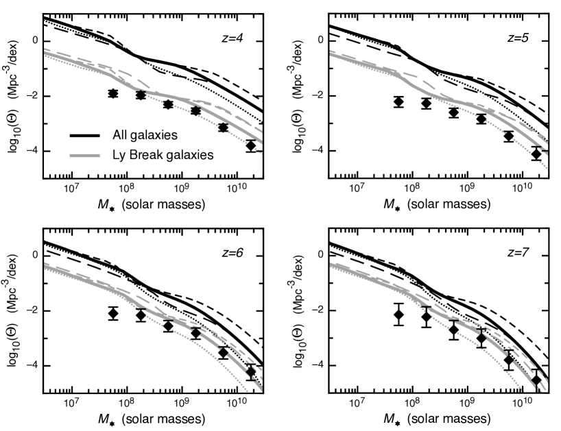
Figure 7: The stellar mass function of a Ly-break selected sample. This is plotted as the grey curves in the attached figure. These curves are for the same models as Figures 3-8. The data points are from González et al. (2011). We also calculate the mass function that would be seen if the sample were selected in stellar mass rather than SFR. The black curves show these models, which are a factor of 5 to 10 higher.

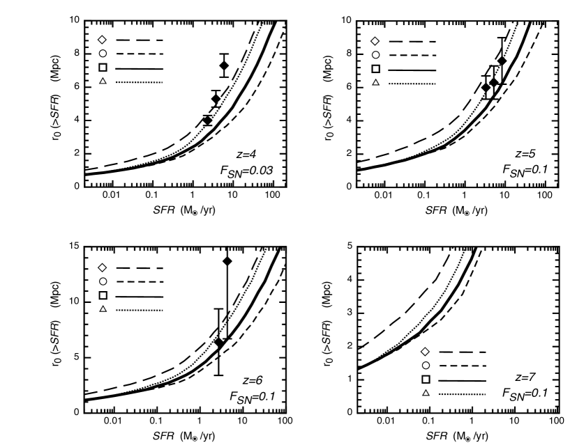
Figure 8: The correlation length in samples above a limiting SFR. The data points are from Lee et al. (2009) and Overzier et al. (2006). The correlation length was calculated for each sample above the limiting star-formation rate by averaging over correlation functions weighted by the SFR density function. Clearly, our model predictions are in good agreement with current observational clustering measurements at $z\sim 5-6$, providing an independent verification of the viability of the model. At $z\sim 4$, our models underestimate the clustering strength somewhat, which may indicate that a smooth contribution to the star formation is required at lower redshifts in a population of more massive, biased halos.

The next observable that we consider is the stellar mass function. Observationally, the stellar mass function at $z~{}\hbox to0.0pt{$>$\hss}{\lower 4.30554pt\hbox{$\sim$}}4$ is currently derived for star-forming, UV-bright, Ly-break selected galaxies. This can be estimated from our model as

$$\Theta(M_{\star})=\Phi(SFR)\times\left(\frac{dSFR}{dM_{\star}}\right)=\Phi(SFR)\times sSFR\\ .$$ (14)

The resulting stellar mass function is plotted as the grey curves in Figure 7 for the models shown in Figure 3-8. The data points are from González et al. (2011). Since our model produces both the correct specific star formation rate and the correct SFRD function, it is no surprise that the agreement is good. This agreement is in contrast to many hydrodynamical models of galaxy formation, in which the constant accretion leads to high duty cycles, and hence a SFR to halo mass ratio which is too low. This low mass-to-light ratio in turn results in a stellar mass function that is too steep.

The low duty-cycle of our bursty model predicts the existence of many galaxies of large stellar mass that are not star forming, and which may therefore be missing from a Ly-break selected stellar mass function. Using our model we therefore also calculate the predicted mass function in the case where the sample was selected based on stellar mass rather than on SFR. This is

$$\Theta_{\rm all}(M_{\star}) = \frac{1}{\epsilon_{\rm duty,tot}}\Phi(SFR)\times\left(\frac{dSFR}{dM_{\star}}\right)$$ (15)

$$= \frac{1}{\epsilon_{\rm duty,tot}}\Phi(SFR)\times sSFR$$

$$= \frac{1}{\epsilon_{\rm duty,tot}}\times\Theta(M_{\star}).$$

In Figure 7 we show the resulting predicted stellar mass functions for the models shown in Figure 3-8 (black curves). Owing to the low duty-cycle, these curves are a factor of $\sim 5-10$ higher than the Ly-break selected case, indicating that high redshift surveys may currently be missing most of the stellar mass produced at early times.

4.6 Clustering of star forming galaxies

Finally, to check whether the relationship between halo mass and SFR is correctly reproduced in our model we calculate the correlation length in samples above a limiting SFR for the four models in this paper. The results are plotted in Figure 8. The correlation length is calculated for a sample above the limiting star-formation rate by averaging over correlation functions weighted by the SFR density function. For comparison we also include clustering measurements from Lee et al. (2009) and Overzier et al. (2006). To convert from an apparent magnitude limit to an intrinsic star formation rate, we assumed a flat SED with $\beta=-2$ for computation of a K-correction, and a conversion from UV luminosity to SFR using Kennicutt (1998). We find that the clustering length increases rapidly towards high SFRs, in agreement with observations. Our model yields a clustering length in the best fit model which is consistent with clustering measurements at $z\sim 5-6$, but underestimates observations at $z\sim 4$. This underestimate may indicate that a smooth contribution to the star formation is required at lower redshifts which would require a population of more massive, biased halos.

5 The Observability of a Passive High-Redshift Population

As outlined above, due to the low effective duty cycle, our model predicts a significant population of galaxies that is not star-forming at a given point in time and might therefore be missed by current high-redshift surveys, which are only sensitive to the rest-frame UV. An accurate estimate for the extent of this missing population should be derived through detailed spectral energy distribution modelling of the whole galaxy population, which is beyond the scope of this paper. However, we briefly outline the likely impact of a low duty cycle and bursty star formation history on the observability of the full galaxy population at high redshift.

There are two ways for a non-starforming galaxy at high-redshift to be missed in a Lyman-break selected sample. Firstly, because the UV luminosity could dim below the detection limit of a survey, and secondly the UV continuum colour could evolve too far to the red where the effective survey volume of a typical LBG selection drops significantly for sources with UV continuum slopes $\beta~{}\hbox to0.0pt{$>$\hss}{\lower 4.30554pt\hbox{$\sim$}}-1$. In practice however, the drop in the UV luminosity is likely the main cause for a galaxy not being selected. Based on simple star-formation histories with short star-formation times ($t_{\mathrm{SF}}<100$ Myr) and using Bruzual & Charlot (2003) stellar population models, one finds that a galaxy dims by an order of magnitude (i.e. 2.5 mag) in the rest-frame UV light after $~{}\hbox to0.0pt{$<$\hss}{\lower 4.30554pt\hbox{$\sim$}}100$ Myr of a passive phase. Given the star formation lifetime of $t_{\rm SF}\sim 10^{7}$ yr and duty-cycle of $\sim 10\%$, this value of $\sim 100$ Myr is comparable to, but shorter than the average time between bursts in our model at $z>4$, leading to sources being missed from current surveys. Furthermore, after 100 Myr, a galaxy’s rest-frame UV continuum slope would have reddened by $\Delta\beta>1$, which would further diminish its chance to be selected as a robust high-redshift source.

Our model therefore predicts a significant population of UV faint galaxies with red UV continuum slopes of $\beta~{}\hbox to0.0pt{$>$\hss}{\lower 4.30554pt\hbox{$\sim$}}-1$. Such sources could in principle be searched for based on $Spitzer$/IRAC imaging which samples rest-frame optical wavelengths of $z\sim 4-8$ sources. In the rest-frame optical, a galaxy would only dim by $\sim 1.5$ mag after 100 Myr without star formation. Such galaxies would be detectable in the deepest current IRAC images over the Hubble Ultra-Deep Field (reaching down to $\sim 27$ mag_AB; see Oesch et al., 2013) out to $z\sim 6$ if their stellar masses are a few times 10${}^{9}M_{\odot}$. However the selection of such galaxies is complicated by possible contamination from very dusty low-redshift sources (see e.g. Caputi et al., 2012; Wiklind et al., 2008), as well as by confusion due to the broad IRAC point-spread function. The advent of JWST will, therefore, greatly facilitate the identification of passive high-redshift sources due to its higher resolution and much better sensitivity in several filters sampling the observed $>2~{}\mu$m regime, and will for the first time enable a full census of high-redshift galaxies.

6 Discussion

In this paper we have described a bursty model for SNe regulated high redshift star formation. Our model successfully reproduces the star-formation selected stellar mass function because it predicts both the star formation rate density function and the correct specific star formation rate of star forming galaxies. However, if we are considering the stellar mass function of the whole galaxy population then there is stellar mass missing from the observed census. Indeed, based on our model, we argue that surveys currently find only $\sim 10-20\%$ of the total stellar mass density at $z\ga 4$.We argue that the low duty-cycle of star formation in this model produces possible solutions to two observed puzzles in high redshift galaxy formation.

The first puzzle relates to the observation that the specific star-formation rate does not evolve significantly with redshift or mass at $z\geq 4$, in contrast to theoretical expectation. Our bursty model naturally produces this behaviour. We point out that the value of the specific star formation rate, and its observed evolution at high redshift directly constrain the duty-cycle (averaged over a Hubble time) of high redshift star-formation to be approximately 10%, independent of a specific model for star-formation.

The second puzzle lies in the relation between the observed growth of stellar mass and the observed instantaneous star formation rate. The stellar mass density that is directly observed in samples at high redshift is the stellar mass density in the population of star forming galaxies (González et al., 2011). This quantity may be different from the total stellar mass density in the Universe. There seems to be disagreement between the relationship of star formation rate to stellar mass observed at $z\sim 6$ (Bouwens et al., 2011) and at $z\sim 2-4$ (Wilkins et al., 2008). Specifically, at $z\sim 2-4$, Wilkins et al. (2008) find that there is not enough growth in stellar mass to account for all of the star-formation observed. Wilkins et al. (2008) calculate the stellar mass density ($\rho_{\rm\star,obs}$) using fits to the stellar mass function, and take the derivative across a redshift interval $\Delta z\sim 0.5$ to find an inferred star formation rate $\dot{\rho}_{\rm\star,inf}$ in units of mass per time per Mpc³. Comparing with the observed star formation rate $\dot{\rho}_{\rm\star,obs}$ at $z\sim 2-4$, Wilkins et al. (2008) found that $\dot{\rho}_{\rm\star,obs}>\dot{\rho}_{\rm\star,inf}$ with a difference of $\sim 0.6$ dex. However with a duty-cycle smaller than unity, the stellar mass in the star forming galaxies was built up over a time shorter than the survey depth, meaning that $\rho_{\rm\star,inf}$ is an overestimate relative to the observed stellar mass. In this case only a fraction $\epsilon_{\rm duty}$ of galaxies with stellar mass $M_{\star}$ are observed in a particular survey, but all galaxies would have starbursts during a time corresponding to the survey depth (note this does not imply that the instantaneous SFRD is underestimated). Thus, if a Ly-break is needed to identify the galaxies in which stellar mass is observed, much of the stellar mass at a particular time would be missed by the survey since it is contained in non-star forming galaxies. The difference is a factor of inverse the duty-cycle, explaining the disagreement between observed and inferred quantities found by Wilkins et al. (2008). We note that if the galaxy sample were selected on stellar mass rather than on UV luminosity, the estimates of star formation rate density based on instantaneous SFRD and the derivative of stellar mass density would agree.

In a complementary analysis Bouwens et al. (2011) have taken the stellar mass function at $z\sim 6-8$ determined by González et al. (2011) and differentiated to get the star formation rate in a survey at $z>6$. However, in contrast to the results of Wilkins et al. (2008) at $z\sim 2-4$, in this higher redshift case the resulting stellar mass is found to agree well with the stellar mass inferred directly. At first sight this is a failure for our model, which predicts that these estimates should differ by a factor of inverse duty-cycle as they do at lower redshift. The solution to this apparent contradiction lies in the fact that at $z\sim 6-8$ the survey depth of $\Delta z\sim 0.5$ corresponds to a time difference across the survey that is similar to the starburst lifetime (but shorter than the time between major mergers), in contrast to the case at $z\sim 2-4$ where $\Delta z\sim 0.5$ corresponds to a time that is longer than the star-burst lifetime.

Thus, in difference to observations at $z\sim 2-4$, at $z\ga 6$ we expect that the observed galaxies had star formation episodes for a time that is similar to the survey depth, meaning that the stellar mass census within star forming galaxies does include all the stellar mass that was generated during the survey depth time interval. As a result, in the $z\ga 6$ samples, integrating the observed star formation rate between the upper and lower redshifts of the survey gives a stellar mass that approximately equals the mass observed in those $z\sim 6$ galaxies, in agreement with the comparison of Bouwens et al. (2011) (see also Robertson et al., 2013). However this equivalence is a coincidence, and does not correspond to a large duty cycle. Rather, galaxies that are not star forming, and therefore not seen in the survey did not form stars during the survey interval. Thus as in the $z\sim 2-4$ case, there is additional stellar mass in quiescent galaxies that is not accounted for in the observed stellar mass function.

We note that this finding is in contrast to recent work at $z\la 3$ that has used the UltraVISTA survey to construct a K-selected catalog covering masses $M_{\star}\ga 10^{11}$M_⊙ (Muzzin et al., 2013; Ilbert et al., 2013). These authors find stellar mass functions selected by stellar mass to agree reasonably well with UV selected samples, and that star-forming galaxies dominate the stellar mass density at low redshift. This would indicate that $z\la 3$ UV selections are not necessarily missing too many galaxies at the very massive end of the population. At $z\ga 4$ our model is not consistent with this behaviour, which is indicative of a larger duty-cycle or a component of continuous star-formation. Full SED modelling of a galaxy population based on merger trees will be required to understand all the observational selection effects on the observability of the predicted non-star forming galaxy population from our model in detail.

7 Conclusion

We have shown that a bursty model of high redshift star formation reproduces a range of observations of the high redshift galaxy population. In particular, we point out that the observed specific star formation rate requires a duty-cycle of $\sim 10\%$, which follows directly from the fact that the observed star formation rate in galaxies integrated over a Hubble time exceeds the observed stellar mass by an order of magnitude. We use this observational constraint to calibrate the efficiency of feedback in a model for the high redshift star formation rate which includes merger driven star formation regulated by SNe feedback. This model reproduces the star formation rate density function and the stellar mass function of galaxies at $4\la z\la 7$.

The finding of a $\sim 10\%$ duty cycle implies that there are ten times the number of known galaxies at fixed stellar mass that have not yet been detected. Since current observations select galaxies by their UV luminosity, and hence only detect star-forming galaxies without too much extinction, our model predicts a large undetected population of UV-faint galaxies that accounts for most of the stellar mass density at $z=4-8$. Unfortunately, at $z>4$ there are currently no good constraints on non star-forming galaxies. These UV faint galaxies would be detectable through their rest-frame optical emission with the Spitzer Space Telescope or JWST. However, it is difficult to define selection criteria that select such sources without significant contamination from lower redshift dusty galaxies (Caputi et al., 2012; Wiklind et al., 2008). The existence of a large population of undetected galaxies which are not forming stars would not affect the global star formation rate history or inferences about the reionization of the intergalactic medium (IGM), but would affect the estimated cumulative stellar mass as a function of redshift and the number density of passive galaxies at each redshift.

Acknowledgments JSBW acknowledges the support of an Australian Research Council Laureate Fellowship. AL was supported in part by NSF grant AST-0907890 and NASA grants NNX08AL43G and NNA09DB30A. PO acknowledges support by NASA through Hubble Fellowship grant HF-51278.01 awarded by the Space Telescope Science Institute, which is operated by the Association of Universities for Research in Astronomy, Inc., for NASA, under contract NAS 5- 26555.

References

- Barkana & Loeb (2001) Barkana R., Loeb A., 2001, ApJS, 349, 125
- Bell & de Jong (2001) Bell E. F., de Jong R. S., 2001, ApJ, 550, 212
- Bouwens et al. (2011) Bouwens R. J., Illingworth G. D., Oesch P. A., Labbé I., Trenti M., van Dokkum P., Franx M., Stiavelli M., Carollo C. M., Magee D., Gonzalez V., 2011, ApJ, 737, 90
- Bruzual & Charlot (2003) Bruzual G., Charlot S., 2003, MNRAS, 344, 1000
- Caputi et al. (2012) Caputi K. I., Dunlop J. S., McLure R. J., Huang J.-S., Fazio G. G., Ashby M. L. N., Castellano M., et al. 2012, ApJL, 750, L20
- Clarke & Oey (2002) Clarke C., Oey M. S., 2002, MNRAS, 337, 1299
- Dekel & Woo (2003) Dekel A., Woo J., 2003, MNRAS, 344, 1131
- Ellis et al. (2013) Ellis R. S., McLure R. J., Dunlop J. S., Robertson B. E., Ono Y., Schenker M. A., Koekemoer A., Bowler R. A. A., Ouchi M., Rogers A. B., Curtis-Lake E., Schneider E., Charlot S., Stark D. P., Furlanetto S. R., Cirasuolo M., 2013, ApJL, 763, L7
- Finlator et al. (2011) Finlator K., Oppenheimer B. D., Davé R., 2011, MNRAS, 410, 1703
- Gonzalez et al. (2012) Gonzalez V., Bouwens R., llingworth G., Labbe I., Oesch P., Franx M., Magee D., 2012, ArXiv e-prints
- González et al. (2011) González V., Labbé I., Bouwens R. J., Illingworth G., Franx M., Kriek M., 2011, ApJL, 735, L34
- González et al. (2010) González V., Labbé I., Bouwens R. J., Illingworth G., Franx M., Kriek M., Brammer G. B., 2010, ApJ, 713, 115
- Ilbert et al. (2013) Ilbert O., McCracken H. J., Le Fèvre O., Capak P., Dunlop J., Karim A., Renzini M. A., Caputi K., et al. 2013, A&A, 556, A55
- Jaacks et al. (2012) Jaacks J., Nagamine K., Choi J.-H., 2012, ArXiv e-prints
- Kauffmann et al. (2003) Kauffmann G., Heckman T. M., White S. D. M., Charlot S., Tremonti C., Peng E. W., Seibert M., Brinkmann J., Nichol R. C., SubbaRao M., York D., 2003, MNRAS, 341, 54
- Komatsu et al. (2011) Komatsu E., Smith K. M., Dunkley J., Bennett C. L., Gold B., Hinshaw G., Jarosik N., Larson D., et al. 2011, ApJS, 192, 18
- Lacey & Cole (1993) Lacey C., Cole S., 1993, MNRAS, 262, 627
- Lee et al. (2012) Lee K.-S., Ferguson H. C., Wiklind T., Dahlen T., Dickinson M. E., Giavalisco M., Grogin N., Papovich C., Messias H., Guo Y., Lin L., 2012, ApJ, 752, 66
- Lee et al. (2009) Lee K.-S., Giavalisco M., Conroy C., Wechsler R. H., Ferguson H. C., Somerville R. S., Dickinson M. E., Urry C. M., 2009, ApJ, 695, 368
- Loeb & Furlanetto (2012) Loeb A., Furlanetto S., 2012, Princeton University Press, Chapter 10
- McLure et al. (2012) McLure R. J., Dunlop J. S., Bowler R. A. A., Curtis-Lake E., Schenker M., Ellis R. S., Robertson B. E., Koekemoer A. M., Rogers A. B., Ono Y., Ouchi M., Charlot S., Wild V., Stark D. P., Furlanetto S. R., Cirasuolo M., Targett T. A., 2012, ArXiv e-prints
- Mo et al. (1998) Mo H. J., Mao S., White S. D. M., 1998, MNRAS, 295, 319
- Muñoz & Loeb (2011) Muñoz J. A., Loeb A., 2011, ApJ, 729, 99
- Muzzin et al. (2013) Muzzin A., Marchesini D., Stefanon M., Franx M., McCracken H. J., Milvang-Jensen B., Dunlop J. S., Fynbo J. P. U., Le Fevre O., Brammer G., Labbe I., 2013, ArXiv e-prints
- Neistein & Dekel (2008) Neistein E., Dekel A., 2008, MNRAS, 383, 615
- Oesch et al. (2012) Oesch P. A., Bouwens R. J., Illingworth G. D., Gonzalez V., Trenti M., van Dokkum P. G., Franx M., Labbé I., Carollo C. M., Magee D., 2012, ApJ, 759, 135
- Oesch et al. (2013) Oesch P. A., Bouwens R. J., Illingworth G. D., Labbé I., Franx M., van Dokkum P. G., Trenti M., Stiavelli M., Gonzalez V., Magee D., 2013, ApJ, 773, 75
- Oesch et al. (2013) Oesch P. A., Labbe I., Bouwens R. J., Illingworth G. D., Gonzalez V., Franx M., Trenti M., Holden B. P., van Dokkum P. G., Magee D., 2013, ApJ, 772, 136
- Oey & Clarke (1997) Oey M. S., Clarke C. J., 1997, MNRAS, 289, 570
- Overzier et al. (2006) Overzier R. A., Bouwens R. J., Illingworth G. D., Franx M., 2006, ApJL, 648, L5
- Press & Schechter (1974) Press W. H., Schechter P., 1974, ApJ, 187, 425
- Raičević et al. (2011) Raičević M., Theuns T., Lacey C., 2011, MNRAS, 410, 775
- Robertson et al. (2013) Robertson B. E., Furlanetto S. R., Schneider E., Charlot S., Ellis R. S., Stark D. P., McLure R. J., Dunlop J. S., Koekemoer A., Schenker M. A., Ouchi M., Ono Y., Curtis-Lake E., Rogers A. B., Bowler R. A. A., Cirasuolo M., 2013, ApJ, 768, 71
- Salvaterra et al. (2011) Salvaterra R., Ferrara A., Dayal P., 2011, MNRAS, 414, 847
- Scalo (1998) Scalo J., 1998, in Gilmore G., Howell D., eds, The Stellar Initial Mass Function (38th Herstmonceux Conference) Vol. 142 of Astronomical Society of the Pacific Conference Series, The IMF Revisited: A Case for Variations. p. 201
- Sheth & Tormen (1999) Sheth R. K., Tormen G., 1999, MNRAS, 308, 119
- Smit et al. (2012) Smit R., Bouwens R. J., Franx M., Illingworth G. D., Labbé I., Oesch P. A., van Dokkum P. G., 2012, ArXiv e-prints
- Smit et al. (2013) Smit R., Bouwens R. J., Labbe I., Zheng W., Bradley L., Donahue M., Lemze D., et al. 2013, ArXiv e-prints
- Stark et al. (2009) Stark D. P., Ellis R. S., Bunker A., Bundy K., Targett T., Benson A., Lacy M., 2009, ApJ, 697, 1493
- Stark et al. (2013) Stark D. P., Schenker M. A., Ellis R., Robertson B., McLure R., Dunlop J., 2013, ApJ, 763, 129
- Trenti et al. (2010) Trenti M., Stiavelli M., Bouwens R. J., Oesch P., Shull J. M., Illingworth G. D., Bradley L. D., Carollo C. M., 2010, ApJL, 714, L202
- Weinmann et al. (2011) Weinmann S. M., Neistein E., Dekel A., 2011, MNRAS, 417, 2737
- Wiklind et al. (2008) Wiklind T., Dickinson M., Ferguson H. C., Giavalisco M., Mobasher B., Grogin N. A., Panagia N., 2008, ApJ, 676, 781
- Wilkins et al. (2008) Wilkins S. M., Trentham N., Hopkins A. M., 2008, MNRAS, 385, 687
- Wyithe & Loeb (2003) Wyithe J. S. B., Loeb A., 2003, ApJ, 595, 614
- Wyithe & Loeb (2013) Wyithe J. S. B., Loeb A., 2013, MNRAS, 428, 2741