Energy-density-functional calculations including the proton-neutron mixing

Abstract

We present results of calculations based on the Skyrme energy density functional including the arbitrary mixing between protons and neutrons. In this framework, single-particle states are superpositions of proton and neutron components and the energy density functional is fully invariant with respect to three-dimensional rotations in the isospin space. The isospin of the system is controlled by means of the isocranking method, which carries over the standard cranking approach to the isospin space. We show numerical results of the isocranking calculations performed for isobaric analogue states in the $A=14$ and $A=40-56$ nuclei. We also present such results obtained for high-isospin states in ⁴⁸Cr, with constraints on the isospin implemented by using the augmented Lagrange method.

The superfluidity and superconductivity phenomena manifest themselves at different physical scales in condensed matter, nuclear, and elementary particle physics. They reflect the universality of the underlying Bardeen-Cooper-Schrieffer (BCS) mechanism of forming Cooper pairs and pair condensates, irrespective of details of attractive interactions at the Fermi energy. In atomic nuclei, which are composite systems built of two types of fermions interacting strongly in charge independent way, the BCS mechanism offers a unique possibility to form, apart of conventional neutron-neutron and proton-proton Cooper pairs, also the proton-neutron (p-n) pairs of isoscalar ($T=0$) or isovector ($T=1$) type.

Although the attempts to incorporate the p-n pairing into the independent-quasi-particle approach date back to the late sixties, see Refs. [Goo79] ; [Per04w] and Refs. quoted therein for a review, a consistent theory of nuclear pairing in the vicinity of the $N=Z$ line, where the p-n correlations are expected to be strongest, is still missing. The reason is that the existing approaches concentrate on introducing the p-n pairing mixing on top of unmixed proton and neutron single-particle (s.p.) orbitals. However, a consistent approach to the problem of the p-n pairing requires implementing the p-n mixing on the mean-field (MF) level, whereby the s.p. wave functions are linear combinations of proton and neutron components. Basic self-consistency principles require such mixing to accompany any anticipated p-n mixing on the pairing level. Moreover, the stability and existence of the p-n pairing condensate may critically depend on the restoring force related to the p-n mixing on the MF level, and thus, to obtain meaningful estimates of the effect, in the theoretical description both must be simultaneously included.

Our ultimate goal is to develop a consistent symmetry-unrestricted energy-density-functional (EDF) approach including the p-n mixing both in the pairing (p-p) and particle-hole (p-h) channels, with rigorous treatment of the isospin degree of freedom, which is of vital importance for the understanding of elementary excitations along the $N=Z$ line. In this work, being a first step in achieving our goal, we report on a development of the EDF approach based on extended Skyrme EDF including the p-n mixing in the p-h channel, with the isospin degree of freedom controlled by means of three-dimensional isocranking model.

The calculations performed below are based on a local Skyrme EDF generalized to include the p-n mixing according to the general rules given by Perlińska et al. [Per04w] . At present we consider only scalar-isoscalar EDFs preserving both the rotational and isospin symmetries but further generalizations are rather straightforward. The explicit form of the employed EDF is given in Eqs. (39), (40), (62), and Table I of Ref. [Per04w] . This model, hereinafter referred to as pnEDF, was implemented within the HFODD code (v2.56e) [Sch12s] solving the nuclear Skyrme-Hartree-Fock(-Bogoliubov) problem by using the Cartesian deformed harmonic-oscillator basis.

Since the model breaks distinction between proton and neutron orbitals, the underlying Kohn-Sham equations must be solved in $A$-dimensional space, where $A$ denotes the number of nucleon. The neutron and proton numbers $N,Z$ or, alternatively, the third component of the isospin $T_{z}$, must be fixed by additional constraints. This is achieved by adding the isocranking term to the MF Hamiltonian [Sat01] :

$$\hat{h}^{\prime}=\hat{h}-\vec{\lambda}\cdot\hat{\vec{t}},$$ (1)

where $\hat{\vec{t}}$ denotes the s.p. isospin operator. The isocranking model is analogous to that used successfully in the standard tilted-axis-cranking calculations for high-spin states and can be viewed as the lowest-order approximation to isospin projection in a sense of Kamlah expansion [Kam68] . By changing the isocranking frequency $\vec{\lambda}$, we can control the magnitude and direction of the isospin of the system. In the following, we shall show numerical results of the isocranking calculations for selected isobaric multiplets. In all calculations we shall use the SkM* parameter set of Ref. [Bar82s] .

For pedagogical reasons, we begin the discussion with the isocranking calculations without Coulomb interaction, which is the only source of the isospin-symmetry breaking in our model. Indeed, at present we disregard the proton-neutron mass difference as well as any hadronic charge-dependent and charge-symmetry-violating terms, and thus we limit ourselves to a purely isoscalar EDF. Hence, as long as the Coulomb energy is switched off, the model Hamiltonian is invariant under rotations in the isospace and the total and s.p. energies become independent of the direction of the isospin, whereas the s.p. wave functions all acquire common p-n mixing coefficients. This property considerably simplifies the physics, helps to verify the validity of the code, and, in particular, helps to work out a strategy of adjusting the isocranking frequency.

The absolute value (length) of the isocranking frequency is determined from the results of the standard EDF calculation without the p-n mixing for non-zero isospin states. The key role is played by the isoaligned states, $T_{z}=\pm T$, in the isobaric multiplet. In even-even nuclei these states correspond to ground-states, which are uniquely defined by occupying pairwise the Kramers degenerated levels from the bottom of the potential well and are very well represented by p-n unmixed Slater determinants [Sat09a] . Hence, in the first step, we perform standard EDF calculation for the ground state of $T=T_{z}$ nucleus and find the difference between the proton and neutron Fermi energies. The difference sets the length of the isocranking frequency as $|\vec{\lambda}|=\lambda_{z}$. With this choice the resulting proton and neutron Fermi energies roughly coincide, because the isocranking term, $-\lambda_{z}\hat{t}_{z}$, raises the proton s.p. energies by $\lambda_{z}/2$ and lowers the neutron energies by $-\lambda_{z}/2$. Next, by keeping the value of $\lambda=|\vec{\lambda}|$ fixed, we change gradually the direction of $\vec{\lambda}$ from $\theta=0^{\circ}$ to $\theta=180^{\circ}$ where $\theta$ denotes the polar angle of $\vec{\lambda}$,

$$\vec{\lambda}=(\lambda\sin\theta,0,\lambda\cos\theta).$$ (2)

In this way we gradually reduce $T_{z}$ or, alternatively, decrease $N$ and increase $Z$. The results are entirely independent of the azimuthal angle $\phi$ in the isospace.

The procedure is illustrated for a representative example of $A=48$ nuclei. In Fig. 1(a), we plot the total energies of the $T=2$ and $T=4$ states in $A=48$ nuclei obtained within the isocranking calculations together with that of the $T=0$ state (the ground state of ⁴⁸Cr). For the $T=2$ and $T=4$ states, we take the standard EDF solutions of ⁴⁸Ti and ⁴⁸Ca, respectively, as initial states and iteratively solve the isocranking pnEDF equations. The direction of isospin is controlled by changing the direction of $\vec{\lambda}$ while keeping its magnitude $|\vec{\lambda}|$ fixed and equal to 11 MeV (6 MeV) for $T=4$ $(T=2)$, respectively. Let us recall that these values are inferred from the differences in proton and neutron Fermi energies obtained in the p-n unmixed EDF calculations in ⁴⁸Ca and ⁴⁸Ti, respectively. Going from ⁴⁸Ca ($T_{z}=4$) to ⁴⁸Ni ($T_{z}=-4$) or from ⁴⁸Ti ($T_{z}=2$) to ⁴⁸Fe ($T_{z}=-2$), $\vec{\lambda}$ draws a semicircle trajectory ($\theta=0^{\circ}\rightarrow 180^{\circ}$) whose radius is $|\vec{\lambda}|$ with the center at the origin. Fig. 1(a) shows the results for different values of the polar angles of isocranking frequency $\theta$. No p-n mixing takes place in the states with $T=|T_{z}|$, such as ⁴⁸Ca ($T=T_{z}=4$), ⁴⁸Ti ($T=T_{z}=2$) ⁴⁸Ni ($T=-T_{z}=4$), ⁴⁸Fe ($T=T_{z}=2$), and ⁴⁸Cr ($T=T_{z}=0$). These correspond to either $\theta=0^{\circ}$ or $180^{\circ}$.

In these calculations, the azimuthal angle $\phi$ was set to $0^{\circ}$. We have confirmed that the results do not depend on $\phi$ even if the Coulomb interaction is included. This is so, because the Coulomb interaction is aligned along the $T_{z}$ axis and thus commutes with isorotations around this axis. Therefore, in what follows the isocranking is investigated only in the $T_{z}-T_{x}$ ($\lambda_{z}-\lambda_{x}$) plane. This choice has an additional advantage of avoiding the time-reversal symmetry breaking inherent to isorotations along the $T_{y}$ axis, see discussion in Ref. [Per04w] .

The procedure outlined above can also be used to calculate odd-$T$ states, see also Fig. 1 in Ref. [Sat01a] . In $A=4n$ cases it would require to carry out first the standard EDF calculation for an odd-odd nucleus with $T=T_{z}$, e.g., in ${}^{48}_{21}$Sc₂₇ for the $A=48$ isobars discussed above. Having the initial state, the odd-$T$ multiplet can be calculated by following essentially the same isocranking procedure as used for the even-$T$ cases. However, the calculation of odd (odd-odd) nuclei involves breaking of the time-reversal symmetry. In order to avoid complications caused by the time-reversal symmetry non-conservation which, among the others, creates ambiguities in configuration assignment of the initial state we shall concentrate here on the isobaric multiplets obtained by applying isocranking to the ground states of even-even $T=|T_{z}|$ nuclei that preserve the time-reversal symmetry. In $A=4n+2$ nuclei, this assumption will limit our calculations to odd-$T$ isobaric multiplets. In particular, in odd-odd $N=Z$ nuclei, it will allow us to represent the $T=1$ IASs by means of a single time-symmetry-conserving (anti-aligned in space) Slater determinant. More general situations will be discussed elsewhere.

In Fig. 1(a) we plot the IASs obtained by isocranking the $T=T_{z}$ states. As expected from the isospin symmetry, the energy curves are flat, that is, independent of the direction of the isospin or value of $T_{z}$. We have independently verified that the non-zero isospin states shown in Fig. 1(a) can be obtained by isocranking the initial $T=0$ state, that is, by starting with the $T=0$ state and performing the $T_{x}$-axis isocranking. Then, the term $-\lambda_{x}\hat{t}_{x}$ gives vertical excitations: $T=0\rightarrow T=2\rightarrow T=4$ with $\langle\hat{T}_{z}\rangle=0$. Similarly, the $T_{z}$-axis isocranking term, $-\lambda_{z}\hat{t}_{z}$, applied to the same $T=0$ state produces a sequence of diagonal excitations: $T=0\rightarrow T=2\rightarrow T=4$ with $T=|\langle\hat{T}_{z}\rangle|$. Irrespective of the direction of the isocranking axis, one always obtains only even-$T$ states. This is because, owing to the time-reversal symmetry, with increasing isocranking frequency only a configuration change with $\Delta T=2$ occurs at each level crossing. To obtain odd-$T$ states, explicit 1p-1h excitations are required [Sat01] .

Figure 1(b) shows s.p. Routhians, that is, the eigenenergies of $\hat{h}^{\prime}$ (1), calculated for $T=4$ states as functions of $\langle\hat{T}_{z}\rangle$. We can clearly see that they are independent of $\langle\hat{T}_{z}\rangle$. The Routhians are pure proton or neutron s.p. states only at $\theta=0^{\circ}$ and $180^{\circ}$. At all other tilting angles $0^{\circ}<\theta<180^{\circ}$ the Routhians are p-n mixed.

Quantitative features of the p-n mixing are listed in Table 1 for the two highest occupied s.p. spherical orbitals. In the discussion it is enough to focus on one state, say, the $f_{7/2}$ state, which, at $\theta=0^{\circ}$, corresponds to a pure neutron state. Gradual tilting of the isorotation axis increases proton component of the state, which, at $\theta=90^{\circ}$, reaches exactly 50%. Eventually, at $\theta=180^{\circ}$ the state becomes a pure proton state. This result applies to all orbitals, which interchange their character from pure proton/neutron at $\theta=0^{\circ}$ to pure neutron/proton at $\theta=180^{\circ}$ and are fifty-fifty mixed exactly at $\theta=90^{\circ}$. It is worth stressing that when the Coulomb interaction is switched off, the total isospin is exactly parallel to $\vec{\lambda}$. Moreover, the isospin of each s.p. state is either parallel or anti-parallel to $\vec{\lambda}$. The s.p. eigenstates of Eq. (1) are, at the same time, the eigenstates of $\hat{h}$, whose eigenvalues are also independent of $\langle\hat{T}_{z}\rangle$. As we shall see later, these features occur only when the Coulomb interaction is neglected.

Figure 1: (Color online) (a) Energies of the $T=0$, 2, and 4 states in $A=48$ isobars obtained by the isocranking calculation without the Coulomb interaction as functions of $\langle\hat{T}_{z}\rangle$. (b) The s.p. Routhians for $|\vec{\lambda}|=11$ MeV ($T=4$ states) calculated without the Coulomb interaction as functions of $\langle\hat{T}_{z}\rangle$. There is no p-n mixing at $T_{z}=4$ and -4, where each s.p. orbital is either proton ($\pi$) or neutron ($\nu$) state. Note that the $\pi$-$\nu$ character at $T_{z}=-4$ is opposite to that at $T_{z}=4$.

Table 1: Calculated expectation values of twice the isospin operators $2\hat{t}_{x}$ and $2\hat{t}_{z}$ for the two highest occupied orbitals of the $T=4$ states in $A=48$ isobars. The Coulomb interaction is switched off. The expectation values of the $T_{x}$ and $T_{z}$ components of the total isospin as well as its polar angles $\theta_{T}$ are also shown.

$\theta$		$0^{\circ}$	$60^{\circ}$	$90^{\circ}$	$120^{\circ}$	$180^{\circ}$
$\theta_{T}$		$0^{\circ}$	$60^{\circ}$	$90^{\circ}$	$120^{\circ}$	$180^{\circ}$
$f_{7/2}$	$\langle\hat{\tau}_{x}\rangle$	0.00	0.87	1.00	0.87	0.00
	$\langle\hat{\tau}_{z}\rangle$	1.00	0.50	0.00	-0.50	-1.00
$d_{3/2}$	$\langle\hat{\tau}_{x}\rangle$	0.00	-0.87	-1.00	-0.87	0.00
	$\langle\hat{\tau}_{z}\rangle$	-1.00	-0.50	0.00	0.50	1.00
$\langle\hat{T}_{x}\rangle$		0.00	3.46	4.00	3.46	0.00
$\langle\hat{T}_{z}\rangle$		4.00	2.00	0.00	-2.00	-4.00

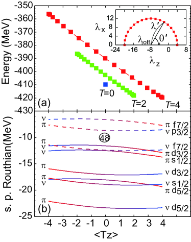
Figure 2: (Color online) (a) Energies of the $T\simeq 0$, 2, and 4 states in $A=48$ isobars obtained by the isocranking calculation with the Coulomb interaction included. Results for every 10^∘ of $\theta^{\prime}$ are plotted. The inset shows the isocranking frequencies used for the $T\simeq 4$ calculation in the $\lambda_{x}-\lambda_{z}$ plane. (b) Same as Fig. 1(b) but with the Coulomb interaction included.

Table 2: Same as Table I but calculated with the Coulomb interaction. Note that the polar angles $\theta$ of $\vec{\lambda}$, defined in Eq. (2) are very different from the polar angles $\theta^{\prime}$ of $\vec{\lambda}^{\prime}$, defined in Eq. (3), and that the latter are close to the polar angles $\theta_{T}$ of $\langle\hat{\vec{T}}\rangle$.

$\theta$		$0^{\circ}$	$100.9^{\circ}$	$108.4^{\circ}$	$133.9^{\circ}$	$180^{\circ}$
$\theta^{\prime}$		$0^{\circ}$	$60^{\circ}$	$90^{\circ}$	$120^{\circ}$	$180^{\circ}$
$\theta_{T}$		$0^{\circ}$	$62.3^{\circ}$	$90.3^{\circ}$	$118.0^{\circ}$	$180^{\circ}$
$f_{7/2}$	$\langle\hat{\tau}_{x}\rangle$	0.00	0.89	1.00	0.88	0.00
	$\langle\hat{\tau}_{z}\rangle$	1.00	0.46	0.01	-0.47	-1.00
$d_{3/2}$	$\langle\hat{\tau}_{x}\rangle$	0.00	-0.90	-1.00	-0.88	0.00
	$\langle\hat{\tau}_{z}\rangle$	-1.00	-0.44	0.00	0.47	1.00
$\langle\hat{T}_{x}\rangle$		0.00	3.54	4.00	3.53	0.00
$\langle\hat{T}_{z}\rangle$		4.00	1.86	-0.02	-1.88	-4.00

Next, we discuss calculations performed with the Coulomb interaction included and treated exactly both in the direct and exchange channels [Dob09ds] . To reduce the Coulomb repulsion, the Coulomb interaction always tends to increase (decrease) the neutron (proton) components of all states; therefore states with larger values of $\langle T_{z}\rangle$ are always energetically favored. Moreover, the s.p. Routhians now vary as functions of the tilting angle $\theta$, and in the interval of $0^{\circ}\leq\theta\leq 180^{\circ}$ many level crossings may take place. This often becomes a source of the ping-pong divergence during the iteration [Dob00c] , rising technical difficulties in the applications.

A simple and efficient prescription to avoid the level crossings of Routhians is to parametrize the isocranking frequencies as

$$\vec{\lambda}=(\lambda^{\prime}\sin\theta^{\prime},0,\lambda^{\prime}\cos\theta^{\prime}+\lambda_{\rm off}).$$ (3)

The semicircle trajectory, which we introduced above, is now shifted in the $T_{z}$-direction of the isospace by the offset value of $\lambda_{\rm off}$, as depicted in the inset of Fig. 2(a). The rationale for this choice is in the fact that the Coulomb interaction depends on the $T_{z}$-component of the isospin. It can thus be regarded as an effective additional contribution to the isocranking term in the $T_{z}$-direction. The offset $\lambda_{\rm off}$ in Eq. (3) is added to compensate for this additional contribution.

In practice, we proceed as follows: First, we perform the standard EDF calculation for the $T\simeq|T_{z}|$ nuclei, so as to specify the endpoints $\lambda_{\rm off}\pm\lambda^{\prime}$ at $\theta^{\prime}=0^{\circ}$ and $180^{\circ}$. Again, they are determined from the differences of the proton and neutron Fermi energies, as was the case without the Coulomb interaction. For example, in the representative example of the $T\simeq 4$ states in $A=48$ isobars, in ⁴⁸Ca we obtain $\lambda_{n}-\lambda_{p}\simeq 4$ MeV, and in ⁴⁸Ni we obtain $\lambda_{n}-\lambda_{p}\simeq-20$ MeV. Hence, we take $\lambda_{\rm off}=-8$ and $\lambda^{\prime}=12$ MeV . The same procedure applied to $T\simeq 2$ multiplet gives $(\lambda_{\rm off},\lambda^{\prime})=(-8.0,6.4)$ MeV.

Figure 2(a) shows calculated energies of the $T\simeq 0,2$, and 4 multiplets in $A=48$ isobars. Approximate linear dependence of the total energies on $\langle\hat{T}_{z}\rangle$ results from a dominance of the isovector part of the Coulomb interaction, over its isotensor component, in the isospin symmetry-breaking mechanism. In terms of the Coulomb energy, which macroscopically behaves as $Z^{2}=T_{z}^{2}-AT_{z}+A^{2}/4$, this fact reflects a dominant role of the linear term $-AT_{z}$. It is worth stressing that, in the presence of the isospin-symmetry breaking fields, the rotation in the isospace becomes nonuniform. Indeed, as shown in Table 2, the direction of isospin is no longer parallel to $\vec{\lambda}$ (angle $\theta$). However, the direction of the shifted cranking axis $\vec{\lambda}^{\prime}$ (angle $\theta^{\prime}$) is approximately parallel with the direction of the isospin meaning that the use of shifted semicircle can be viewed as effective way of restoring the isospin symmetry in the vicinity of the Fermi energy.

The usefulness of the shifted semicircle technique is illustrated in Fig. 2(b) and Fig. 3(a). Fig. 2(b) shows the s.p. Routhians in function of $\langle\hat{T}_{z}\rangle$ calculated for the $T\simeq 4$ states in $A=48$ isobars. In this case, the endpoint nuclei ${}^{48}_{28}$Ca₂₀ and ${}^{48}_{20}$Ni₂₈ are doubly-magic. The shifted semicircle method causes the neutron and proton Fermi energies and, in turn, the proton and neutron magic gaps, to match one another, independently, to a large extent, of values of $\langle\hat{T}_{z}\rangle$. As a result, for all values of $\langle\hat{T}_{z}\rangle$, a sizable gap at $A=48$ stays open in the s.p. spectrum and the crossings are avoided. Fig. 3(a) shows the results obtained for the $T\simeq 4$ multiplets in $A=40-56$ isobars. Systems with $|T_{z}|=4$ and $A\neq 48$ are not magic nuclei, so there is no large shell gap at the Fermi surface in their s.p. spectra. Nevertheless, the shifted semicircle method works nicely.

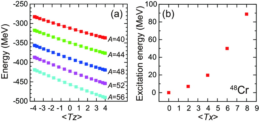
Figure 3: (Color online) Left, energies of the $T\simeq 4$ states in $A=40-56$ isobars with even $A/2$ as functions of $\langle\hat{T}_{z}\rangle$. For $A=40$, 44, 48, 52, and 56, we used the values of $(\lambda_{\rm off},\lambda^{\prime})=(-6.8,13.6)$, $(-7.4,12.4)$, $(-8.0,12.0)$, $(-8.4,11.6)$, and $(-8.8,12.4)$ MeV, respectively. Right, excitation energies of ⁴⁸Cr for $\langle\hat{T}_{x}\rangle=0$, 2, 4, 6, and 8, calculated by using the augmented Lagrange method.

The isocranking calculations are based on a simple linear constraint method, whereupon fixed values of the isocranking frequencies $\vec{\lambda}$ or $\vec{\lambda}^{\prime}$ lead, in general, to non-integer values of $\langle\hat{T}_{z}\rangle$. To improve on that, we also implemented in our code a method for optimization with constraints, known as the augmented Lagrange method [Sta10] ; [Sch12s] , which is widely used in quantum chemistry. Using this method, one can obtain states with $\langle\hat{T}_{z}\rangle$ having exactly integer values. In Fig. 3(b), we plot the excitation energies of the $T\simeq 0$, 2, 4, 6, and 8 states of ⁴⁸Cr, calculated with the augmented Lagrange method. In these calculations, we employed the constraints on $\langle\hat{T}_{z}\rangle=0$ and $\langle\hat{T}_{x}\rangle=0$, 2, 4, 6 ,and 8, respectively. The obtained (quasi)parabolic behavior of the calculated energies is determined mostly by the nuclear symmetry energy. One should bear in mind, however, that the energies along the parabola also depend on shell effects, manifesting themselves, among the other, in rapid shape changes. The calculated quadrupole deformations for states with $\langle\hat{T}_{x}\rangle=0$, 2, 4, 6, and 8 are equal to $\beta_{2}=0.27$, 0.19, 0, 0.07, and 0, respectively. The latter four values are in perfect agreement with the ground state equilibrium deformations calculated directly by using the EDF method in the ⁴⁸Ti, ⁴⁸Ca, ⁴⁸Ar, and ⁴⁸S nuclei, respectively, which are their $T\simeq T_{z}$ IASs. This constitutes an explicit illustration of the fact that the isospin symmetry and isospin quantum number, albeit approximate, are very powerful concepts in nuclear structure.

To conclude, we consider the case of $A=4n+2$ nuclei, focusing our attention on the well-known $I=0^{+},T=1$ triplet of states in the $A=14$ isobars [Boh69] . Here, two members of the triplet, namely the $I=0^{+},T\simeq|T_{z}|=1$ ground states of ¹⁴C and ¹⁴O nuclei are represented in our model by the standard EDF ground states without the p-n mixing. Their $T_{z}=0$ IAS representing the excited $I=0^{+},T=1$ state in ¹⁴N, is calculated by using the isocranking model, and is described by a single time-even Slater determinant built of s.p. p-n mixed orbitals. Let us recall that in the case of $A=4n+2$ nuclei the odd-$T$ states are represented as the time-even Slater determinants, whereas the even-$T$ states break the time-reversal symmetry.

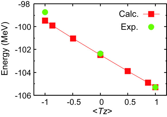
Figure 4: (Color online) Energies of $T\simeq 1$ states in $A=14$ isobars in comparison with the experimental data [Brookhaven] . The calculated energies are shifted by 3.2 MeV such that the experimental and calculated binding energies of ¹⁴C coincide. The results of isocranking calculations for every $30^{\circ}$ of $\theta^{\prime}$ between $\theta^{\prime}=0^{\circ}$ and $180^{\circ}$ are plotted.

The calculated energies and the corresponding experimental data are depicted in Fig. 4. To correct for a deficiency of the SkM* EDF, which overestimates the binding energy of ¹⁴C, the entire theoretical curve is shifted up by 3.2 MeV. In ¹⁴N, the calculated state, representing the excited $0^{+},T=1$ state (the IAS with $T_{z}=0$), is described by a single Slater determinant built of the p-n mixed s.p. states. The isocranking calculation correctly reproduce its energy relative to the IAS with $T_{z}=1$. This proves that the model is indeed capable of quantitatively describing the excitation energies of the $0^{+},T=1$ IASs. This can be contrasted with single-reference p-n unmixed EDF models, wherein such states do not exist at all [Sat10] .

In summary, for the first time we solved the generalized Skyrme Kohn-Sham equations including the arbitrary mixing of protons and neutrons. Values of the average total isospin and its $T_{x}$, $T_{y}$, and $T_{z}$ components were controlled by using the isocranking approximation. The model was applied to the isobaric analogue states in even-even $A=40-56$ and odd-odd $A=14$ isobars. We have demonstrated that the p-n mixed single-reference EDF approach is capable of quantitatively describing the isobaric analogue excited states. Of particular importance are the $I=0^{+},T=1,T_{z}=0$ states in odd-odd $N=Z$ nuclei because of their participation in the superallowed Fermi beta decay that is used to test the Standard Model of particle physics [Tow10] . We have also shown the results of the augmented Lagrange method for high-isospin states in ⁴⁸Cr. Such calculations can be used to study the nuclear symmetry energy.

This work is a first step toward the EDF calculations including the p-n mixing in both p-p and p-h channels. Such simultaneous mixing in both channels is required by fundamental self-consistency arguments. When implemented, it will allow us to reexamine, from a completely new perspective, the fundamental questions concerning formation and stability of static p-n pairing correlations, coexistence of different condensates, microscopic nature of the Wigner energy and properties of the symmetry energy in paired systems.

As discussed in Ref. [Sat10] , the MF approach is affected by spurious isospin mixing, which can be quantified and removed by performing the isospin projection and subsequent Coulomb rediagonalization. The implementation of the isospin projection of pnEDF states is now in progress. Furthermore, by using the technology of iterative methods [Nak07a] ; [Ina09x] ; [Toi10s] ; [Avo11] ; [Sto11s] ; [Car12a] ; [Hin13] , we plan to construct an efficient numerical code solving equations of the quasiparticle random phase approximation based on the p-n mixed EDF. This may open new possibilities of investigating collective excitations of the isobaric analogue states and charge-exchange reactions to/from these states.

This work was partly supported by JSPS KAKENHI (Grant numbers 20105003, 21340073, and 25287065), by the Academy of Finland and University of Jyväskylä within the FIDIPRO programme, and by the Polish National Science Center under Contract No. 2012/07/B/ST2/03907. The numerical calculations were carried out on SR16000 at Yukawa Institute for Theoretical Physics in Kyoto University and on RIKEN Integrated Cluster of Clusters (RICC) facility. We also acknowledge the CSC - IT Center for Science Ltd, Finland, for the allocation of computational resources.

References

- [1] A.L. Goodman, Adv. Nucl. Phys. 11, 263 (1979).
- [2] E. Perlińska et al., Phys. Rev. C 69, 014316 (2004).
- [3] N. Schunck et al., Comput. Phys. Commun. 183, 166 (2012); J. Dobaczewski et al., to be published.
- [4] W. Satuła and R. Wyss. Phys. Rev. Lett. 86, 4488 (2001); 87, 052504 (2001).
- [5] A. Kamlah, Z. Phys. 216, 52 (1968).
- [6] J. Bartel et al., Nucl. Phys. A386, 79 (1982).
- [7] W. Satuła, J. Dobaczewski, W. Nazarewicz, and M. Rafalski, Phys. Rev. Lett. 103, 012502 (2009).
- [8] W. Satuła and R. Wyss, Acta Phys. Pol. B 32, 2441 (2001).
- [9] J. Dobaczewski et al., Comput. Phys. Commun. 180, 2361 (2009).
- [10] J. Dobaczewski and J. Dudek, Comput. Phys. Commun. 131, 164 (2000).
- [11] A. Staszczak, M. Stoitsov, A. Baran, and W. Nazarewicz, Eur. Phys. J. A 46, 85 (2010).
- [12] A. Bohr and B.R. Mottelson, Nuclear Structure (Benjamin, New York, 1969), Vol. I.
- [13] National Nuclear Data Center, Brookhaven National Laboratory, http://www.nndc.bnl.gov/.
- [14] W. Satuła, J. Dobaczewski, W. Nazarewicz, and M. Rafalski, Phys. Rev. C 81, 054310 (2010).
- [15] I.S. Towner and J.C. Hardy, Phys. Rev. C 82, 065501 (2010).
- [16] T. Nakatsukasa, T. Inakura, and K. Yabana, Phys. Rev. C 76, 024318 (2007).
- [17] T. Inakura, T. Nakatsukasa, and K. Yabana, Phys. Rev. C 80, 044301 (2009); Phys. Rev. C 84, 021302 (2011).
- [18] J. Toivanen et al., Phys. Rev. C 81, 034312 (2010).
- [19] P. Avogadro and T. Nakatsukasa, Phys. Rev. C 84, 014314 (2011).
- [20] M. Stoitsov et al., Phys. Rev. C 84, 041305 (2011).
- [21] B.G. Carlsson, J. Toivanen, and A. Pastore, Phys. Rev. C 86, 014307 (2012).
- [22] N. Hinohara, M. Kortelainen, and W. Nazarewicz, arXiv:1304.4008.