Calculation of the Autocorrelation Function of the Stochastic Single Machine Infinite Bus System

Abstract

Critical slowing down (CSD) is the phenomenon in which a system recovers more slowly from small perturbations. CSD, as evidenced by increasing signal variance and autocorrelation, has been observed in many dynamical systems approaching a critical transition, and thus can be a useful signal of proximity to transition. In this paper, we derive autocorrelation functions for the state variables of a stochastic single machine infinite bus system (SMIB). The results show that both autocorrelation and variance increase as this system approaches a saddle-node bifurcation. The autocorrelation functions help to explain why CSD can be used as an indicator of proximity to criticality in power systems revealing, for example, how nonlinearity in the SMIB system causes these signs to appear.

I Introduction

Insufficient stability monitoring and situational awareness have been identified as critical contributors to recent large power system failures, such as August 14, 2003 [1] and Sept. 8, 2011 [2]. Recent deployment of phasor measurement units (PMU) produce large quantities of time-series data, which open tremendous opportunities to improve power system stability monitoring and control. However doing so requires algorithms and methods that transform these data into useful information about power system stability.

To address this problem, this paper draws from research on critical transitions in stochastic dynamical systems. The statistics of time-series data change notably in most stochastic dynamical systems as they approach critical transitions; systems are more easily perturbed from equilibrium, and take longer to return after being displaced [3], [4]. Collectively, this phenomenon is known as Critical Slowing Down (CSD), and is most easily observed by testing for autocorrelation and variance in time-series data. Increasing autocorrelation and variance have been shown to indicate proximity to critical transitions in climate models [5], ecosystems [6] and the human brain [7]. In prior work by the authors [8], CSD has been shown to be an early warning sign of critical transition in power systems. A deep understanding of CSD in power systems could lead to new tools for wide area measurement and control.

In many systems with critical transitions, slow-varying continuous parameters cause gradual trends in state variables, which generally move the system closer to, or further from, unstable operating points. Simultaneously, random perturbations cause fast changes. As a result, such systems have two time scales: fast and slow. In power systems, loads have slow predictable trends, such as load ramps in the morning hours, and fast stochastic ones, such as random load switching. Whereas conventional generators tend to vary slowly, intermittent renewable generation, such as PV on a partly cloudy day, can have fast stochastic changes. Because of this, the mathematical framework of fast-slow systems [9] and stochastic differential equations [10] can help to explain phenomena in these systems, such as the manner in which autocorrelation and variance increase with proximity to critical points. In [9], the variance and autocorrelation of state variables for several prototypical fast-slow systems is calculated using the Fokker-Planck approach and numerical simulations.

Estimating the proximity of a power system to a particular critical transition (e.g., voltage collapse) has been the focus of a number of papers in the power systems literature. References [11]-[14] present methods to measure the distance between an operating condition and voltage collapse with respect to slow-moving state variables, such as load. While these methods provide useful information about system stability, they require accurate network models all of which contain some error.

Another approach to estimating the distance to critical transitions is to identify statistical patterns in the response of a system to stochastic forcing, such as fluctuations in load, or production from renewable energy sources. To this end, a growing number of papers study power system stability using stochastic models [15]-[18]. Reference [15] models power systems using Stochastic Differential Equations (SDEs) and solves the SDEs using It$\hat{o}$ calculus to develop a measure of voltage security. In [10], the Euler and Milstein methods for numerically solving SDEs are used to assess transient stability in power systems, given fluctuating loads and random faults. Reference [18] uses the time evolution of the probability density function for state variables in a Single Machine Infinite Bus (SMIB) system to show how random load fluctuations affect system stability.

The results above clearly show that power system stability is affected by noise in the system. However, more work is needed to identify useful statistical trends in high sample-rate measurements from power systems. Results from the literature on CSD suggest that the combination of both increased autocorrelation and variance in time-series data are needed in order to gain insight into the proximity to critical transitions from data. Reference [8] provides empirical evidence of increasing autocorrelation and variance for an SMIB model and the 9-bus test case. Reference [19] shows that voltage variance at the end of a distribution feeder increases as it approaches voltage collapse. However, these results do not provide insight into autocorrelation. To our knowledge, only [20] derives an approximate analytical autocorrelation function (from which either autocorrelation or variance can be found) for state variables in a power system model. However, the autocorrelation function in [20] is limited to the operating regime very close to the threshold of instability. In this paper, we derive exact autocorrelation functions for the state variables of an SMIB system. The results provide insight into the conditions under which autocorrelation and variance signal proximity to critical transitions in power systems. We use the results to explain why CSD occurs in power systems, and describe conditions under which autocorrelation and variance signal proximity to critical transitions.

The rest of the paper is organized as follows. Section II provides a brief review of SDEs and solution methods. Section III describes our model, analytical and numerical results. Section IV discusses the implications for power system operations, and Sec. V summarizes the results and contributions of this paper.

II A Brief Review of Stochastic Differential Equations

There are two different approaches to modeling and solving Stochastic Differential Equations (SDEs): the It$\hat{o}$ and the Stratonovich interpretations. In the It$\hat{o}$ interpretation [21], noise is considered to be uncorrelated, whereas in the Stratonovich interpretation [22] noise has finite, albeit very small, correlation time [23]. It$\hat{o}$ calculus is often used in discrete systems, such as finance, though a few papers have applied the It$\hat{o}$ approach to power systems [15], [10]. On the other hand, the Stratonovich method is often used in continuous physical systems where noise is band-limited [24]. The Stratonovich interpretation also facilitates the use of ordinary calculus, which is not possible under the It$\hat{o}$ interpretation.

In this paper we organize our model to use the multivariate Ornstein-Uhlenbeck stochastic differential equation, as described in [23]:

$$d\underline{Z}\left(t\right)=A\underline{Z}\left(t\right)dt+Bd\mathbf{\underline{\textrm{W}}}\left(t\right)$$ (1)

where $\underline{Z}\left(t\right)$ is the vector of the state variables, $A$ and $B$ are constant matrices, and $\underline{W}\left(t\right)$ represents an $n$-dimensional Wiener process. The increments of the Wiener process ($d\underline{W}(t)$) are independent, normally distributed random variables, such that:

$$\underline{W}\left(t_{i}\right)-\underline{W}\left(t_{i-1}\right)\sim\mathcal{N}\left(0,t_{i}-t_{i-1}\right)$$ (2)

Because $B$ is a constant matrix in this paper, the It$\hat{o}$ and Stratonovich interpretations result in the same solution [24]. We will follow the Stratonovich interpretation because it allows for the use of ordinary calculus.

III Stochastic Single Machine Infinite Bus System

Analysis of small power system models can be very helpful for understanding the concepts of power system stability. The single machine infinite bus system has long been used for this purpose. Reference [25] explores the small signal stability of synchronous machines using the SMIB system. In [26], Wang et al. use a novel control technique to improve the transient stability and voltage regulation of a SMIB system. In the recent literature, there is increasing interest in stochastic analysis of power systems, in part due to the increasing integration of variable renewable energy sources. A few of these papers use stochastic SMIB models. In [27], it is suggested that increasing noise in the stochastic SMIB system can make the system unstable and induce chaotic behavior. Reference [18] (mentioned in Sec. I) also studied stability in a stochastic SMIB system.

In this section, we derive autocorrelation functions of the state variables for a stochastic SMIB system. Analysis of these functions provides analytical evidence for, and insight into, CSD in a small power system.

III-A Stochastic SMIB System Model

Fig. 1 shows an stochastic SMIB system. Equation (3), which combines the mechanical swing equation and the electrical power produced by the generator, fully describes the dynamics of this system:

$$M\ddot{\delta}+D\dot{\delta}+\frac{(1+\eta)E^{\prime}_{a}}{X}\sin\left(\delta\right)=P_{m}$$ (3)

where $(\eta\sim\mathcal{N}(0,0.01))$ is a white Gaussian random variable added to the voltage magnitude of the infinite bus to account for the noise in the system, $M$ and $D$ are the combined inertia constant and damping coefficient of the generator and turbine, and $E_{a}^{{}^{\prime}}$ and $\delta$ are the transient emf and the rotor angle of the generator. The rotor angle is the angle difference between the rotor position and a synchronously rotating reference axis. The reactance $X$ is the sum of the generator transient reactance $(X_{d}^{{}^{\prime}})$ and the line reactance $\left(X_{l}\right)$, and $P_{m}$ is the input mechanical power. The third term in the left-hand side of (3) is the generator’s electrical power $\left(P_{g}\right)$. In order to test the system with varying amounts of stress, we solved the system for different equilibria, considering that generator’s mechanical and electrical power are equal at each equilibrium:

$$P_{m}=P_{g0}=\frac{E_{a}^{{}^{\prime}}}{X}\sin\left(\delta_{0}\right)$$ (4)

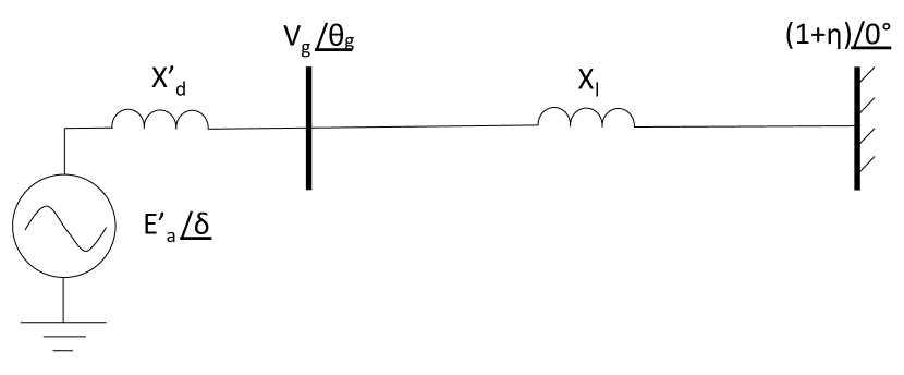
Figure 1: Stochastic single machine infinite bus system model used in sec. III.

III-B Autocorrelation and Variance of the Differential Variables

In order to solve (3) analytically, we linearized it around the equilibrium point using the first-order Taylor expansion:

$$\Delta\ddot{\delta}+\frac{D}{M}\Delta\dot{\delta}+\frac{E^{\prime}_{a}}{MX}\cos\left(\delta_{0}\right)\Delta\delta=-\frac{\eta}{M}P_{g0}$$ (5)

where $\delta_{0}$ is the value of the rotor angle at the equilibrium, and $\Delta\delta$ is the deviation of the rotor angle from its mean value. Equation (6) is the standard form of (5), which is known as the damped harmonic oscillator equation with noisy forcing:

$$\ddot{Z}+2\gamma\dot{Z}+\omega_{0}^{2}Z=-f\eta$$ (6)

for which the following equalities hold:

$$Z=\Delta\delta;\gamma=\frac{D}{2M};\omega_{0}=\sqrt{\frac{E_{a}^{{}^{\prime}}\cos\delta_{0}}{MX}};f=\frac{P_{g0}}{M}$$ (7)

Equalities in (7) show that $f$ increases with $\delta_{0}$ while $\omega_{0}$ decreases with $\delta_{0}$.

Rewriting (6) as (1) results in a set of two first order SDEs. Here, $\underline{\textrm{Z}}\left(t\right)=\left[\begin{array}[]{cc}\Delta\delta&\Delta\dot{\delta}\end{array}\right]^{T}$ where $\Delta\dot{\delta}$ is the deviation of the generator speed from its mean value, and $\underline{W}(t)$ is a 2-variable Wiener process. The matrices A and B in (1) are as follows:

$$A=\left[\begin{array}[]{cc}0&1\\ -\omega_{0}^{2}&-2\gamma\end{array}\right],\qquad B=\left[\begin{array}[]{cc}0&0\\ 0&-f\end{array}\right]$$ (8)

At $\delta_{0}=\pi/2$, $\omega_{0}$ is equal to zero, so one of the eigenvalues of matrix $A$ becomes zero. As a result, the system experiences a saddle-node bifurcation.

Following the method in [23], the solution of (6) is as follows:

$$\Delta\delta\left(t\right) = f\cdot\int_{-\infty}^{t}[\exp\left(\gamma\left(t^{\prime}-t\right)\right)\eta\left(t^{\prime}\right)$$

$$\hskip 10.00002pt\cdot\frac{\sin\left(\omega^{\prime}(t^{\prime}-t)\right)}{\omega^{\prime}}]dt^{\prime}$$

$$\Delta\dot{\delta}\left(t\right) = f\cdot\int_{-\infty}^{t}[\exp\left(\gamma\left(t^{\prime}-t\right)\right)\eta\left(t^{\prime}\right)$$

$$\quad\cdot\frac{-\sin\left(\omega^{\prime}(t^{\prime}-t)+\phi\right)\omega_{0}}{\omega^{\prime}}]dt^{\prime}$$

where $\omega^{\prime}=\sqrt{\omega_{0}^{2}-\gamma^{2}}$ is the frequency of the underdamped harmonic oscillator, and $\phi=\arctan(\omega^{\prime}/\gamma)$. Note that $\omega^{\prime}$ and $\phi$ decrease with $\delta_{0}$. Using (III-B) and (III-B), we calculated the stationary variances and autocorrelations of $\Delta\delta$, $\Delta\dot{\delta}$. Note that the eigenvalues of $A$ have negative real part before the bifurcation point since $\gamma>0$. The variances are as follows:

$$\sigma_{\Delta\delta}^{2} = \frac{f^{2}\sigma_{\eta}^{2}}{4\gamma\omega_{0}^{2}}$$ (11)

$$\sigma_{\Delta\dot{\delta}}^{2} = \frac{f^{2}\sigma_{\eta}^{2}}{4\gamma}$$ (12)

If $\gamma<\omega_{0}$, which holds until $\delta_{0}\approx\frac{\pi}{2}$ in our system, the autocorrelation functions for $\Delta\delta$ and $\Delta\dot{\delta}$ are as follows:

$$E\left[\Delta\delta\left(t\right)\Delta\delta\left(s\right)\right] = \exp\left(-\gamma\Delta t\right)\frac{f^{2}}{4\gamma\omega^{\prime}\omega_{0}}$$

$$\cdot\sin\left(\omega^{\prime}\Delta t+\phi\right)\sigma_{\eta}^{2}$$

$$E\left[\Delta\dot{\delta}\left(t\right)\Delta\dot{\delta}\left(s\right)\right] = \exp\left(-\gamma\Delta t\right)\frac{-f^{2}\omega_{0}}{4\gamma\omega^{\prime}}$$

$$\cdot\sin\left(\omega^{\prime}\Delta t-\phi\right)\sigma_{\eta}^{2}$$

where $t$ and $s$ are two different times such that $t>s$, and $\Delta t=t-s$.

III-C Numerical example

Using (11)-(III-B), we calculated the variances and autocorrelations of $\Delta\delta$, $\Delta\dot{\delta}$ at different equilibria; see Figs. 2, 3. Here, the bifurcation parameter is the input mechanical power $P_{m}$. The parameters are given below:

$E^{\prime}_{a}=1.2\textrm{pu},D=0.03\frac{\textrm{pu}}{rad/s},H=4\frac{MW.s}{MVA},X_{d}^{\prime}=0.15\textrm{pu,}$

$X_{l}=0.1\textrm{pu},\omega_{s}=2\pi\cdot 60$

Note that $M=2H/\omega_{s}$, where $H$ is the inertia constant, and $\omega_{s}$ is the rated speed in $rad/s$.

Fig. 4 shows the autocorrelation function of $\Delta\delta$ for different values of $P_{m}$. It shows that choosing $\Delta t$ close to 1/4 of the smallest period of the function allows one to observe the monotonic increase of the autocorrelation as $P_{m}$ increases. For larger values of $\Delta t$, the increase of the autocorrelation may not be observed since the frequency of the function’s oscillations varies with $P_{m}$. For smaller values of $\Delta t$, the increase of the autocorrelation is less noticeable since the function curves become closer to each other as the time lag approaches zero. We chose $\Delta t=0.1$s.

In Figs. 2 and 3, the analytical and numerical results are compared with each other. In order to calculate the numerical results, (3) was solved using a fixed-step trapezoidal ordinary differential equation solver. At each time step, $\eta\left(t\right)$ changes according to its normal probability density function. The minimum period of oscillations in this system $(T=2\pi/\omega^{\prime})$ is 0.4 sec. We chose the integration step size to be 0.01 sec which is much shorter than the period of the shortest oscillation. For each equilibrium, we integrated (6) 100 times; the average results are shown in the plots. The numerical results are shown for the range of the bifurcation parameter values for which the numerical solutions were stable. The ratio $q_{4}/q_{1}$ in Figs. 2 and 3 is equal to the value of the variance or autocorrelation for $P_{m}=4\textrm{pu}$ divided by the corresponding value for $P_{m}=1\textrm{pu}$.

Fig. 2 shows that the variances of $\Delta\delta$ and $\Delta\dot{\delta}$ increase with $P_{m}$, and seem to be good indicators of proximity to the bifurcation. However, the growth rates of the two variances are different. The difference becomes more significant near the bifurcation where the variance of $\Delta\delta$ increases much faster than the variance of $\Delta\dot{\delta}$. This is caused by the term $\omega_{0}^{2}$ in the denominator of the expression for the variance of $\Delta\delta$ in (11) . In Fig. 3, the autocorrelations of $\Delta\delta$ and $\Delta\dot{\delta}$ increase with $P_{m}$. Similar to the variances, the autocorrelations are good indicators of proximity to the bifurcation as well.

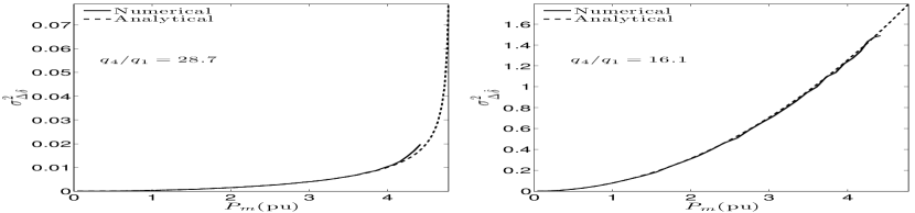
Figure 2: Variance of $\Delta\delta,\Delta\dot{\delta}$ for different mechanical power $(P_{m})$ values.

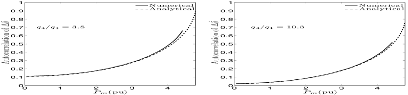
Figure 3: Autocorrelation of $\Delta\delta,\Delta\dot{\delta}$ for different mechanical power $(P_{m})$ values. The autocorrelation values are normalized by dividing by the variances of the variables.

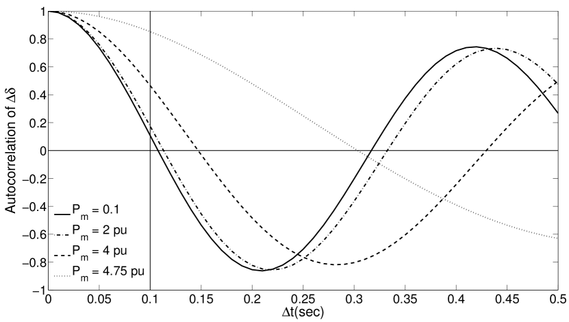
Figure 4: Autocorrelation function of $\Delta\delta$. $\Delta t=0.1$ is close to 1/4 of the smallest period of the function (for different values of $P_{m}$).

III-D Autocorrelation and Variance of the Algebraic Variables

In order to calculate the variance and autocorrelation of the algebraic variables (the generator’s terminal voltage magnitude and angle), we wrote KCL at the generator’s terminal:

$$\frac{E^{\prime}_{a}e^{i\delta}-V_{g}e^{i\theta_{g}}}{jX^{\prime}_{d}}+\frac{1+\eta-V_{g}e^{i\theta_{g}}}{jX_{l}}=0$$ (15)

Separating the real and imaginary parts in (15), gives the following:

$$V_{g}\sin\left(\theta_{g}\right) = \alpha E_{a}^{{}^{\prime}}\sin\left(\delta\right)$$ (16)

$$V_{g}\cos\left(\theta_{g}\right) = \alpha E_{a}^{{}^{\prime}}\cos\left(\delta\right)$$

$$+\left(1+\eta\right)\left(1-\alpha\right)$$

where $\alpha=X_{l}/(X_{l}+X_{d}^{{}^{\prime}})$. Linearizing (16) and (III-D) around the equilibrium results in $\Delta V_{g}$ and $\Delta\theta_{g}$ as linear combinations of $\Delta\delta$ and $\eta$:

$$\Delta V_{g} = \alpha E_{a}^{{}^{\prime}}\sin\left(\theta_{g0}-\delta_{0}\right)\Delta\delta$$

$$+\left(1-\alpha\right)\cos\left(\theta_{g0}\right)\eta$$

$$\Delta\theta_{g} = (\alpha E_{a}^{{}^{\prime}}\cos\left(\theta_{g0}-\delta_{0}\right)\Delta\delta$$

$$-\left(1-\alpha\right)\sin\left(\theta_{g0}\right)\eta)/V_{g0}$$

Then, we rewrote (III-D) and (III-D) as follows:

$$\Delta V_{g} = C_{1}\Delta\delta+C_{2}\eta$$ (20)

$$\Delta\theta_{g} = C_{3}\Delta\delta+C_{4}\eta$$ (21)

where $C_{1},C_{2},C_{3},C_{4}$ are constants that replace the coefficients in (III-D) and (III-D). Then, the autocorrelation of $\Delta V_{g}$ is as follows $\left(t>s\right)$:

$$E\left[\Delta V_{g}\left(t\right)\Delta V_{g}\left(s\right)\right] = C_{1}^{2}\cdot E\left[\Delta\delta\left(t\right)\Delta\delta\left(s\right)\right]$$ (22)

$$+C_{1}C_{2}\mbox{$\cdot$}E\left[\Delta\delta\left(t\right)\eta\left(s\right)\right]$$

In deriving (22), we observed that $E\left[\Delta\delta\left(s\right)\eta\left(t\right)\right]=0$ since the system is causal. Also, $E\left[\eta\left(t\right)\eta\left(s\right)\right]=0$ because $\eta$ is a white random variable. Similarly,

$$E\left[\Delta\theta_{g}\left(t\right)\Delta\theta_{g}\left(s\right)\right] = C_{3}^{2}\cdot E\left[\Delta\delta\left(t\right)\Delta\delta\left(s\right)\right]$$

$$+C_{3}C_{4}\cdot E\left[\Delta\delta\left(t\right)\eta\left(s\right)\right]$$

Equations (22), (III-D) show that in order to calculate the autocorrelation of $\Delta V_{g}$ and $\Delta\theta_{g}$, it is necessary to calculate $E\left[\Delta\delta\left(t\right)\eta\left(s\right)\right]$. We calculated $E\left[\Delta\delta\left(t\right)\eta\left(s\right)\right]$ using (III-B):

$$E\left[\Delta\delta\left(t\right)\eta\left(s\right)\right] = -\exp\left(-\gamma\Delta t\right)\cdot\frac{f}{\omega^{\prime}}$$

$$\cdot\sin\left(\omega^{\prime}\Delta t\right)\sigma_{\eta}^{2}$$

We can infer from (III-D) that $\textrm{cov}\left(\Delta\delta,\eta\right)=0$. As a result, using (11), (III-D) and (III-D), the variances of $\Delta V_{g}$ and $\Delta\theta_{g}$ are as follows:

$$\sigma_{\Delta V_{g}}^{2} = \left(\frac{C_{1}^{2}f^{2}}{4\gamma\omega_{0}^{2}}+C_{2}^{2}\right)\sigma_{\eta}^{2}$$ (25)

$$\sigma_{\Delta\theta_{g}}^{2} = \left(\frac{C_{3}^{2}f^{2}}{4\gamma\omega_{0}^{2}}+C_{4}^{2}\right)\sigma_{\eta}^{2}$$ (26)

Utilizing (III-B), (22), (III-D) and (III-D), we calculated the autocorrelation of $\Delta V_{g}$ :

$$E\left[\Delta V_{g}\left(t\right)\Delta V_{g}\left(s\right)\right] = \exp\left(-\gamma\Delta t\right)\frac{C_{1}f}{4\omega^{\prime}\omega_{0}\gamma}\cdot$$

$$\sqrt{C_{1}f\left(C_{1}f-8C_{2}\gamma^{2}\right)+\left(4C_{2}\omega_{0}\gamma\right)^{2}}$$

$$\cdot\sin\left(\omega^{\prime}\Delta t+\phi_{v_{g}}\right)\cdot\sigma_{\eta}^{2}$$

where $\phi_{v_{g}}=\arctan(\frac{C_{1}f\omega^{\prime}}{C_{1}f\gamma-4C_{2}\gamma\omega_{0}^{2}})$. The autocorrelation function of $\Delta\theta_{g}$ is similar to (III-D) ($C_{1}$ and $C_{2}$ are replaced by $C_{3}$ and $C_{4}$).

Figs. 5,6 show the variance and autocorrelation of $\Delta V_{g},\Delta\theta_{g}$ at different equilibria for this system. In Fig. 5, although the variances of both variables increase with $P_{m}$, the increase of the variance of $\Delta\theta_{g}$ is much more significant. Also, the variance of $\Delta V_{g}$ does not increase with $P_{m}$ until the system gets close to the bifurcation while the variance of $\Delta\theta_{g}$ increases even if the system is far from the bifurcation. Both autocorrelations of $\Delta V_{g}$ and $\Delta\theta_{g}$ in Fig. 6 increase with $P_{m}$. However, the ratio $q_{4}/q_{1}$ is much larger for $\Delta V_{g}$ than $\Delta\theta_{g}$.

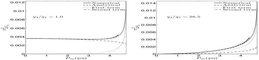
Figure 5: Variance of $\Delta V_{g}$ and $\Delta\theta_{g}$ at different mechanical power $\left(P_{m}\right)$ levels. The two terms comprising the variances in (25) and (26) are also shown.

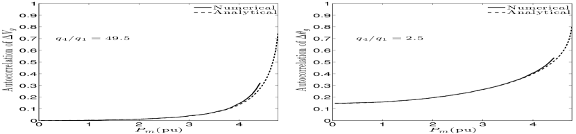
Figure 6: Autocorrelation of $\Delta V_{g}$ and $\Delta\theta_{g}$ versus $P_{m}$.

IV Discussion

Fig. 7 shows the trajectory of the eigenvalues of the state matrix $A$. The system passes through a saddle-node bifurcation as the mechanical power is increased. Near the bifurcation, the eigenvalues are very sensitive to the change of the bifurcation parameter. As a result, the system is in the overdamped regime $(\omega_{0}<\gamma)$ for much less than 0.1% distance in terms of $P_{m}$ to the critical transition. This is consistent with [20], where the autocorrelation function is valid when the system is within 0.1% to the saddle-node bifurcation such that the lowest eigenvalue determines the system dynamics. Accordingly, it can provide a good estimate of the autocorrelation and variance of the system states for a very short range of the bifurcation parameter, but the result of [20] can not be used as an early warning sign.

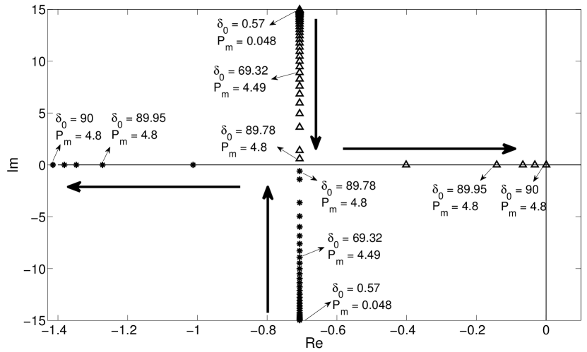
Figure 7: Eigenvalues of the first system as the bifurcation parameter (mechanical power) is increased. The arrows show the direction of the eigenvalues’ movement in the complex plane as $P_{m}$ is increased. The values of $P_{m}$ and $\delta_{0}$ are given for several eigenvalues.

Figs. 2-6 show that the variance and autocorrelation of all four state variables increase when the system is more stressed. This demonstrates that CSD occurs in this system as it approaches the bifurcation, as suggested both general results [9], and prior work for power systems [8, 20].

In addition to validating these prior results, several new observations can be made. For example, the signs of CSD are more clearly observable in some variables, and not others. While all of the variables show some increases in autocorrelation and variance, they are less clearly observable in $\Delta V_{g}$. The variance of $\Delta V_{g}$ decreases with $P_{m}$ slightly until the vicinity of the bifurcation. On the other hand, the variance of $\Delta\theta_{g}$ always increases with $P_{m}$. Fig. 5 shows the two terms in the expressions for $\sigma_{\Delta V_{g}}^{2}$ and $\sigma_{\Delta\theta_{g}}^{2}$, from (25) and (26). The first term in $\sigma_{\Delta V_{g}}^{2}$ is always dominant and growing. On the other hand, the second term in $\sigma_{\Delta V_{g}}^{2}$ is larger for small $P_{m}$. The fact that this term decreases with $P_{m}$ can be observed from $C_{2}$ in (III-D). Accordingly, the decrease of $C_{2}$ with $P_{m}$ causes $\sigma_{\Delta V_{g}}^{2}$ to decrease until $P_{m}$ reaches the vicinity of the bifurcation. With respect to $\sigma_{\Delta\theta_{g}}^{2}$, the second term in (26) increases with $P_{m}$, and adds to the increase caused by the first term. In conclusion, the variance of $\Delta\theta_{g}$ is a better indicator of proximity to the bifurcation.

The results also show that the nonlinearity of this system causes CSD to occur within it. In (8), one of the elements of the state matrix $(-\omega_{0}^{2})$ changes with $P_{m}$ because of the nonlinear relationship between the electrical power $(P_{g})$ and the rotor angle, and that element causes the eigenvalues to change with $P_{m}$. If the relationship between $P_{g}$ and $\delta$ were linear, the state matrix would be constant. In [23], it is shown that the stationary time correlation matrix of (1) can be calculated using the following equation:

$$E\left[\mathbf{\mathbf{\underline{\mathrm{\mathit{Z}}}\left(\mathit{t}\right)}}\underline{Z}{}^{T}\left(s\right)\right]=\exp\left[-A\Delta t\right]\sigma$$ (28)

where $\sigma$ is the covariance matrix of the state variables. From (28), it can be inferred that the normalized autocorrelation matrix only depends on $A$ and the time lag. As a result, if the state matrix is constant, the autocorrelations for an specific time lag will be constant as well. Accordingly, in this system, CSD is caused by the nonlinear relationship between $P_{g}$ and the rotor angle.

Further research is required to design methods that can use CSD to accurately determine whether a particular state is approaching instability in larger power systems. However, the following are some ideas for using this method in a real power system. Using the analytical approaches in this paper in combination with data, we expect to be able to estimate baseline (normal) values for the variance and autocorrelation of system variables. Doing so will require some extension of the analytical approaches in this paper. While it is unlikely that this approach can be used to produce explicit autocorrelation functions, the method should be able to produce numerical values for autocorrelations and variances. Also, using the approach outlined here, the ratio of the statistics in critical conditions to those in normal conditions can be calculated from off-line studies. Using the base values and critical ratios, one can calculate thresholds for CSD signs, which help in informing system operators regarding a critical condition. Calculating autocorrelation and variance from data is not computationally expensive, which makes this method well-suited for real-time application in large power grids.

V Conclusion

In this paper, we derive analytical autocorrelation functions for the state variables in a stochastic single machine infinite bus system. The analytical results were confirmed by numerical simulations. The functions show that this system does indeed express critical slowing down, as evidenced by both increased autocorrelation and variance, before the bifurcation occurs. We also showed that the occurrence of CSD in this system is due to its nonlinearity. Moreover, the results reveal that there are some differences in the growth rate of the CSD signs for different state variables; some variables are better indicators of proximity to the bifurcation than others. These findings suggest ways to better understand CSD in large multi- machine power systems. Understanding the statistical behavior of stochastic power systems as they approach instability should allow for the development of new indicators of power system stability based on the statistical properties of PMU data.

References

- [1] S. Abraham and J. Efford, eds., “Final report on the august 14, 2003 blackout in the United States and Canada: Causes and recommendations,” US-Canada Power System Outage Task Force, Tech. Rep., 2004.
- [2] —, “Arizona-Southern California outages on September 8, 2011: Causes and recommendations,” FERC and NERC Staff, Tech. Rep., Apr. 2012.
- [3] M. Scheffer, J. Bascompte, W. A. Brock, V. Brovkin, S. R. Carpenter, V. Dakos, H. Held, E. H. Van Nes, M. Rietkerk, and G. Sugihara, “Early-warning signals for critical transitions,” Nature, vol. 461, no. 7260, pp. 53–59, Sep. 2009.
- [4] T. Lenton, V. Livina, V. Dakos, E. Van Nes, and M. Scheffer, “Early warning of climate tipping points from critical slowing down: Comparing methods to improve robustness,” Philosophical Transactions of the Royal Society A: Mathematical, Physical and Engineering Sciences, vol. 370, no. 1962, pp. 1185–1204, 2012.
- [5] V. Dakos, M. Scheffer, E. H. van Nes, V. Brovkin, V. Petoukhov, and H. Held, “Slowing down as an early warning signal for abrupt climate change,” Proceedings of the National Academy of Sciences, vol. 105, no. 38, pp. 14 308–14 312, Sep. 2008.
- [6] V. Dakos, S. Kéfi, M. Rietkerk, E. H. van Nes, and M. Scheffer, “Slowing down in spatially patterned ecosystems at the brink of collapse,” The American Naturalist, vol. 177, no. 6, pp. E153–E166, 2011.
- [7] B. Litt, R. Esteller, J. Echauz, M. D’Alessandro, R. Shor, T. Henry, P. Pennell, C. Epstein, R. Bakay, M. Dichter et al., “Epileptic seizures may begin hours in advance of clinical onset: a report of five patients,” Neuron, vol. 30, no. 1, pp. 51–64, 2001.
- [8] E. Cotilla-Sanchez, P. Hines, and C. Danforth, “Predicting critical transitions from time series synchrophasor data,” IEEE Transactions on Smart Grid, vol. 3, no. 4, pp. 1832 –1840, Dec. 2012.
- [9] C. Kuehn, “A mathematical framework for critical transitions: Bifurcations, fast-slow systems and stochastic dynamics,” Physica D: Nonlinear Phenomena, vol. 240, no. 12, pp. 1020–1035, Jun. 2011.
- [10] Z. Y. Dong, J. H. Zhao, and D. Hill, “Numerical simulation for stochastic transient stability assessment,” IEEE Transactions on Power Systems, vol. 27, no. 4, pp. 1741 –1749, Nov. 2012.
- [11] C. A. Canizares et al., “Voltage stability assessment: concepts, practices and tools,” Power System Stability Subcommittee Special Publication IEEE/PES, 2002.
- [12] H. Chiang, I. Dobson, R. J. Thomas, J. S. Thorp, and L. Fekih-Ahmed, “On voltage collapse in electric power systems,” IEEE Transactions on Power Systems, vol. 5, no. 2, pp. 601–611, 1990.
- [13] M. M. Begovic and A. G. Phadke, “Control of voltage stability using sensitivity analysis,” IEEE Transactions on Power Systems, vol. 7, no. 1, pp. 114–123, 1992.
- [14] M. Glavic and T. Van Cutsem, “Wide-area detection of voltage instability from synchronized phasor measurements. part i: Principle,” IEEE Transactions on Power Systems, vol. 24, no. 3, pp. 1408 –1416, Aug. 2009.
- [15] C. De Marco and A. Bergen, “A security measure for random load disturbances in nonlinear power system models,” IEEE Transactions on Circuits and Systems, vol. 34, no. 12, pp. 1546 – 1557, Dec. 1987.
- [16] C. Nwankpa, S. Shahidehpour, and Z. Schuss, “A stochastic approach to small disturbance stability analysis,” IEEE Transactions on Power Systems, vol. 7, no. 4, pp. 1519–1528, Nov. 1992.
- [17] M. Anghel, K. A. Werley, and A. E. Motter, “Stochastic model for power grid dynamics,” in 40th Annual Hawaii International Conference on System Sciences, 2007. IEEE, Jan. 2007.
- [18] K. Wang and M. L. Crow, “The Fokker-Planck equation for power system stability probability density function evolution,” IEEE Transactions on Power Systems, vol. 28, no. 3, 2013.
- [19] M. Chertkov, S. Backhaus, K. Turtisyn, V. Chernyak, and V. Lebedev, “Voltage collapse and ode approach to power flows: Analysis of a feeder line with static disorder in consumption/production,” arXiv preprint arXiv:1106.5003, 2011.
- [20] D. Podolsky and K. Turitsyn, “Random load fluctuations and collapse probability of a power system operating near codimension 1 saddle-node bifurcation,” arXiv preprint arXiv:1212.1224, 2012.
- [21] W. Rümelin, “Numerical treatment of stochastic differential equations,” SIAM Journal on Numerical Analysis, pp. 604–613, 1982.
- [22] R. L. Stratonovich, Introduction to the Theory of Random Noise. Gordon and Breach, 1963.
- [23] C. W. Gardiner, Stochastic Methods: A Handbook for the Natural and Social Sciences, 4th ed. Springer, 2010.
- [24] R. Mannella and V. Peter, “Itô versus stratonovich: 30 years later,” Fluctuation and Noise Letters, vol. 11, no. 01, Mar. 2012.
- [25] F. P. Demello and C. Concordia, “Concepts of synchronous machine stability as affected by excitation control,” IEEE Transactions on Power Apparatus and Systems, vol. PAS-88, no. 4, pp. 316–329, 1969.
- [26] Y. Wang, D. J. Hill, R. H. Middleton, and L. Gao, “Transient stability enhancement and voltage regulation of power systems,” IEEE Transactions on Power Systems, vol. 8, no. 2, pp. 620–627, 1993.
- [27] D. Wei and X. Luo, “Noise-induced chaos in single-machine infinite-bus power systems,” Europhysics Letters, vol. 86, no. 5, p. 50008, 2009.