Nested particle filters for online parameter estimation in discrete–time state–space Markov models

Abstract

We address the problem of approximating the posterior probability distribution of the fixed parameters of a state-space dynamical system using a sequential Monte Carlo method. The proposed approach relies on a nested structure that employs two layers of particle filters to approximate the posterior probability measure of the static parameters and the dynamic state variables of the system of interest, in a vein similar to the recent “sequential Monte Carlo square” (SMC²) algorithm. However, unlike the SMC² scheme, the proposed technique operates in a purely recursive manner. In particular, the computational complexity of the recursive steps of the method introduced herein is constant over time. We analyse the approximation of integrals of real bounded functions with respect to the posterior distribution of the system parameters computed via the proposed scheme. As a result, we prove, under regularity assumptions, that the approximation errors vanish asymptotically in $L_{p}$ ($p\geq 1$) with convergence rate proportional to $\frac{1}{\sqrt{N}}+\frac{1}{\sqrt{M}}$, where $N$ is the number of Monte Carlo samples in the parameter space and $N\times M$ is the number of samples in the state space. This result also holds for the approximation of the joint posterior distribution of the parameters and the state variables. We discuss the relationship between the SMC² algorithm and the new recursive method and present a simple example in order to illustrate some of the theoretical findings with computer simulations.

1308.1883

and

1 Introduction

1.1 Problem statement

The problem of parameter estimation in state-space dynamical systems has received considerable attention, from different viewpoints (Kitagawa, 1998; Liu and West, 2001; Andrieu et al., 2004; Kantas et al., 2015; Carvalho et al., 2010), as it is almost ubiquitous in practical applications. In this paper, we investigate the use of particle filtering methods for the online Bayesian estimation of the static parameters of a state-space system.

In order to ease the discussion, let us consider two (possibly vector-valued) random sequences $\{X_{t}\}_{t=0,1,...}$ and $\{Y_{t}\}_{t=1,2,...}$ representing the (hidden) state of a dynamical system and some related observations, respectively, with $t$ denoting discrete time. We assume that the state process is Markov and the observation $Y_{t}$ is independent of any other observations $\{Y_{k};k\neq t\}$, conditional on the state $X_{t}$. Both the conditional probability distribution of $X_{t}$ given the value of the previous state, $X_{t-1}=x_{t-1}$, and the probability density function (pdf) of $Y_{t}$ given $X_{t}=x_{t}$ are assumed to be known up to a vector of static (random) parameters, denoted by $\Theta$. These assumptions are commonly made in the literature and actually hold for many practical systems of interest (see, e.g., (Ristic, Arulampalam and Gordon, 2004; Cappé, Godsill and Moulines, 2007)). Given a sequence of actual observations, $Y_{1}=y_{1},\ldots,Y_{t}=y_{t},\ldots$, the goal is to track the posterior probability distributions of the state $X_{t}$, $t\geq 0$, and the parameter vector $\Theta$ over time.

In the sequel, we briefly review various existing approaches to the parameter estimation problem that involve particle filtering in some relevant manner. See (Kantas et al., 2015) for a more detailed survey of the field.

1.2 Particle filters and parameter estimation

When the parameter vector is given, i.e., $\Theta=\theta$ is known, the problem reduces to the standard stochastic filtering setting, which consists in tracking the posterior probability distribution of the state $X_{t}$, given the record of observations up to time $t>0$. In a few special cases (e.g., if the system is linear and Gaussian or the state-space is discrete and finite) there exist closed form solutions for the probability distribution of $X_{t}$ given $Y_{1}=y_{1},...,Y_{t}=y_{t}$, which is often termed the filtering distribution. However, analytical solutions do not exist for general, possibly nonlinear and non-Gaussian, systems and numerical approximation methods are then needed. One popular class of such methods are the so-called particle filters (Gordon, Salmond and Smith, 1993; Kitagawa, 1996; Liu and Chen, 1998; Doucet, Godsill and Andrieu, 2000). This is a family of recursive Monte Carlo algorithms that generate discrete random approximations of the sequence of probability measures associated to the filtering distributions at discrete time $t\geq 0$.

Particle filters are well suited for solving the standard stochastic filtering problem. However, the design of particle filters that can account for a random vector of parameters in the dynamic system (i.e., a static but unknown $\Theta$) has been an open issue for the past two decades.

When the system of interest is endowed with some structure, there are some elegant techniques to handle the unknown parameters efficiently. For example, there are various conditionally-linear and Gaussian models that admit the analytical integration of $\Theta$ using the Kalman filter as an auxiliary tool, see, e.g., (Doucet, Godsill and Andrieu, 2000; Chen, Wang and Liu, 2000). A similar approach can be taken with some non-Gaussian models appearing, e.g., in signal processing (Bruno, 2013). In other cases, the analytical integration may not be feasible but the structure of the model can be such that the conditional probability law of $\Theta$ given $X_{0}=x_{0},\ldots,X_{t}=x_{t}$ and $Y_{1}=y_{1},\ldots,Y_{t}=y_{t}$ is tractable. In particular, if $\Theta$ depends on $X_{1:t}=\{X_{1},...,X_{t}\}$ through a low-dimensional sufficient statistic then it is possible to draw efficiently from the posterior distribution of $\Theta$ (given $X_{0:t}=x_{0:t}$ and $Y_{1:t}=y_{1:t}$) (Storvik, 2002; Carvalho et al., 2010) and then integrate the parameters out numerically.

For arbitrary systems, with no particular structure, the more straightforward approach is to augment the state-space by including $\Theta$ as a constant-in-time state variable. This has been proposed in a number of forms and in various applications but it can be shown that standard particle filters working on this augmented state-space do not necessarily converge in general because the resulting systems are non-ergodic (Andrieu et al., 2004; Papavasiliou, 2006). Another popular technique to handle static parameters within particle filtering consists in building a suitable kernel estimator of the posterior probability density function (pdf) of $\Theta$ given $Y_{1:t}=y_{1:t}$ from where new samples in the parameter space can be drawn (Liu and West, 2001). The latter step is often called “rejuvenation” or “jittering” (we adopt the latter term in the sequel). One key feature of this technique is the “shrinkage” of the density estimator in order to control the variance of the jittered particles. This method has been shown to work in some examples with low-dimensional $\Theta$, but has also been found to deliver poor performance in other simple setups (Miguez, Bugallo and Djuric, 2005). A rigorous analysis of this technique is missing as well.

Finally, there exists a large body of research on maximum likelihood estimation (MLE) for unknown parameters. Instead of handling $\Theta$ as a random variable and building an approximation of its posterior distribution, MLE techniques aim at computing a single-point estimate of the parameters. This is typically done by way of gradient optimisation methods, that lend themselves naturally to online implementations. A popular example is the recursive maximum likelihood (RML) algorithm (LeGland and Mevel, 1997; Poyiadjis, Doucet and Singh, 2011; Moral, Doucet and Singh, 2015). As an alternative to gradient search methods, expectation maximization (EM) techniques have also been proposed for the optimisation of the parameter likelihood, both in offline and online versions (Andrieu et al., 2004; Kantas et al., 2015). These techniques use particle filtering as an ancillary tool to approximate either the gradient of the likelihood function (Moral, Doucet and Singh, 2015) or some sufficient statistics (Andrieu et al., 2004) and have been advocated as more robust than those based on state-space augmentation, artificial evolution or kernel density estimation (Andrieu et al., 2004; Kantas et al., 2015).

1.3 Non-recursive methods

A number of new methods related to particle filtering have been proposed in the past few years that tackle the problem of approximating the distribution of the parameter vector $\Theta$ given the observations $Y_{1:T}=y_{1:T}$. These techniques include the iterated batch importance sampling (IBIS) algorithm of (Chopin, 2002) and extensions of it that rely on the nesting of particle methods (such as in (Papavasiliou, 2006) or (Chopin, Jacob and Papaspiliopoulos, 2013)), combinations of Markov chain Monte Carlo (MCMC) and particle filtering (Andrieu, Doucet and Holenstein, 2010), variations of the population Monte Carlo methodology (Koblents and Míguez, 2013) and particle methods for the approximation of the parameter likelihood function (Olsson et al., 2008).

The IBIS method is a sequential Monte Carlo (SMC) algorithm that updates a population of samples $\theta_{t}^{(i)}$, $i=1,...,N$, in the space of $\Theta$, with associated importance weights, at every time step. The technique involves regular MCMC steps, in order to rejuvenate the population of samples, and the ability to compute the pdf of every observation variable $Y_{t}$, given the previous observation record $Y_{1:t-1}=y_{1:t-1}$ and a fixed value of the parameters, $\Theta=\theta$. Let us denote such densities as $d(y_{t}|y_{1:t-1},\theta)$ for the sake of conciseness. The need to obtain $d(y_{t}|y_{1:t-1},\theta)$ in closed-form has two important implications. First, IBIS is not a recursive algorithm, since each time we need to compute $d(y_{t}|y_{1:t-1},\theta)$ for a new sample point $\Theta=\theta$ in the parameter space it is necessary to process the entire sequence of observations $Y_{1:t-1}=y_{1:t-1}$. Second, the algorithm can only be applied when the dynamic model has some suitable structure (e.g., the system may be linear and Gaussian conditional on $\Theta$) that enables us to actually find $d(y_{t}|y_{1:t-1},\theta)$ in closed form.

In (Papavasiliou, 2006), these difficulties with the IBIS method are addressed by using two layers of Monte Carlo methods. First, a random grid of points in the space of $\Theta$, say $\theta^{(1)},...,\theta^{(N)}$, is generated. Then, for each $\Theta=\theta^{(i)}$, $i=1,...,N$, a particle filter is employed targeting the signal $\{X_{t}\}_{t=0,1,...}$. The latter particle filters provide approximations of $d(y_{t}|y_{1:t-1},\theta^{(i)})$, $i=1,...,N$, and, since the grid in the parameter space is fixed, a single sweep over the observations $Y_{1:T}=y_{1:T}$, $T<\infty$, is sufficient, hence the algorithm is recursive. The practical weakness of this approach is that the random grid over the parameter space is generated a priori (irrespective of the observations $Y_{1:T}=y_{1:T}$) and it is not updated as the observations are processed. Therefore, when the prior distribution of $\Theta$ differs from the posterior distribution (of $\Theta$ conditional on $Y_{1:T}=y_{1:T}$) significantly, a very large number, $N$, of samples in the parameter space is needed to guarantee a fair performance.

The methodology proposed in (Chopin, Jacob and Papaspiliopoulos, 2013) is also an extension of the IBIS technique. Similarly to the method in (Papavasiliou, 2006), a random grid is created over the parameter space and a particle filter is run for every node in the grid. However, unlike the technique in (Papavasiliou, 2006), the grid of samples in the space of $\Theta$ is updated over time, as the batch of observations $Y_{1:T}=y_{1:T}$ is processed. In particular, if $\{\theta_{t-1}^{(i)},i=1,...,N\}$ is the grid at time $t-1$, a particle filter is used to process $y_{t}$ and then a new grid $\{\theta_{t}^{(i)},i=1,...,N\}$ can be generated. This filter involves the computation of weights that depend on the densities $d(y_{t}|y_{1:t-1},\theta_{t}^{(i)})$, $i=1,...,N$ (similar to the original IBIS). For each point $\Theta=\theta_{t}^{(i)}$, a particle filter is run to approximate $d(y_{t}|y_{1:t-1},\theta_{t}^{(i)})$. The resulting method is called SMC² in (Chopin, Jacob and Papaspiliopoulos, 2013) because of the two nested layers of particle filters. It is more flexible and general than the original IBIS and its extension in (Papavasiliou, 2006), but it is not a recursive algorithm. New samples in the parameter space are generated by way of particle MCMC (Andrieu, Doucet and Holenstein, 2010) (see below) moves and resampling steps in order to avoid the degeneracy of the particle filter. However, each time a new point in the parameter space is generated at time $t$, say $\theta_{t}^{\prime}$, a new filter has to be run from time 0 to time $t$. Therefore, the computationally complexity of the method grows quadratically with time. A major advantage of the SMC² algorithm is that the approximation errors vanish asymptotically as the number of samples $N$ on the parameter space increases, independently of the number of particles used to approximate the densities $d(y_{t}|y_{1:t-1},\theta_{t}^{(i)})$ in the second layer of particle filters, which can stay fixed. This is shown in (Chopin, Jacob and Papaspiliopoulos, 2013) resorting to a well known unbiasedness property proved in (Del Moral, 2004).

A technique that has quickly gained popularity for parameter estimation is the particle MCMC method of (Andrieu, Doucet and Holenstein, 2010) (employed as a building block for the SMC² method described above). It essentially consists in an MCMC algorithm to approximate the posterior distribution of $\Theta$ given $Y_{1:t}=y_{1:t}$. Such construction is intractable if addressed directly because the likelihoods $d(y_{1:t}|\theta)$ cannot be conmputed exactly. To circumvent this difficulty, it was proposed in (Andrieu, Doucet and Holenstein, 2010) to use particle filters in order to approximate them. The same trick has been used in the population Monte Carlo (Cappé et al., 2004) framework to tackle the approximation of the posterior distribution of $\Theta$ using particles with nonlinearly transformed weights (Koblents and Míguez, 2013). The latter technique has been reported to be computationally more efficient than particle MCMC methods in some examples. These two types of algorithms, as well as the SMC² scheme, revolve around the ability to approximate the factors $d(y_{t}|y_{1:t-1},\theta)$ using particle filtering.

An alternative, and conceptually simple, approach to compute the likelihood of $\Theta$ given $Y_{1:t}$ has been proposed in (Olsson et al., 2008). The problem is addressed by generating a random grid over the parameter space (either random or deterministic, but fixed), then using particle filters to compute the value of the likelihood at each node and finally obtaining an approximation of the whole function by interpolating the nodes. If a point estimate of the parameters is needed, standard optimisation techniques can be applied to the interpolated approximation. Convergence of the $L_{p}$ error norms is proved in (Olsson et al., 2008) for problems where both the parameter space and the state space are compact.

1.4 Contributions

We introduce a particle filtering method for the approximation of the joint posterior distribution of the signal and the unknown parameters, $X_{t}$ and $\Theta$, respectively, given the data $Y_{1:t}=y_{1:t}$. Similar to (Papavasiliou, 2006) and (Chopin, Jacob and Papaspiliopoulos, 2013), the algorithm consists of two nested layers of particle filters: an “outer” filter that approximates the probability measure of $\Theta$ given the observations and a set of “inner” filters, one per sample generated in the outer filter, that yield approximations of the posterior measures that result for $X_{t}$ conditional on the observations and each specific sample of $\Theta$. The outer filter directly provides an approximation of the marginal posterior distribution of $\Theta$, whereas a suitable combination of the latter with the outcomes of the inner filters yields an approximation of the joint posterior probability measure of $X_{t}$ and $\Theta$.

The method is very similar to the SMC² scheme of (Chopin, Jacob and Papaspiliopoulos, 2013) in its structure. However, unlike SMC², it is a purely recursive procedure and, therefore, it is more suitable for an online implementation. At every time step, all the probability measure approximations (both marginal and joint) are updated recursively, with a fixed computational cost. Also, the jittering of particles in the SMC² algorithm is carried out using a particle MCMC kernel (Chopin, Jacob and Papaspiliopoulos, 2013), that leaves the target distribution invariant but cannot be implemented recursively, while the proposed scheme works with simpler Markov kernels easily amenable to online implementations. A detailed comparison between the proposed algorithm and the SMC² method of (Chopin, Jacob and Papaspiliopoulos, 2013) is presented in Section 4.3.

The core of the paper is devoted to the analysis of the proposed algorithm. We study the approximation, via the nested particle filtering scheme, of 1-dimensional statistics of the posterior distribution of the system parameters. Under regularity assumptions, we prove that the $L_{p}$ norms of the approximation errors vanish with rate proportional to $\frac{1}{\sqrt{N}}+\frac{1}{\sqrt{M}}$, where $N$ and $N\times M$ are the number of samples in the parameter space and the number of particles in the state space, respectively. This result also holds for the approximation of the joint posterior distribution of the parameters and the state variables.

The analysis builds upon two basic assumptions, which determine the applicability of the algorithm. The most important one is that the optimal filter for the state space model of interest is continuous with respect to (w.r.t.) the parameter $\theta$, i.e., that small changes to the parameter lead to small changes to the posterior probability measure of the state given the available observations. It is this continuity property that makes the implementation of the proposed recursive algorithm feasible and determines some key practical elements of the algorithm, including the magnitude of the jittering of the particles. Non-recursive methods, such as particle MCMC or SMC², are not subject to this constraint. The second basic assumption is that the parameter space is a compact set and the the conditional pdf of the observations is well behaved (positive and upper bounded) uniformly over that set. The proposed technique is not guaranteed to work if the parameters have to be searched over an infinite support or, most importantly, if the conditional pdf of the observations has some singularity (e.g., it becomes unbounded) for some parameter values.

To complement the analysis, we also provide a numerical example, where we apply the proposed algorithm to jointly track the state variables and estimate the fixed parameters of a (stochastic version of the) Lorenz 63 system. The length of the observation periods for this example ($\sim 40,000$ discrete time steps) is large enough to make the application of the non-recursive SMC² method impractical, while the proposed technique attains accurate estimates of the unknown parameters and tracks the state variables closely.

1.5 Organisation of the paper

We present a general description of the random state-space Markov models of interest in this paper in Section 2, including a brief review of the standard particle filter with known parameters. The recursive nested particle filter scheme is introduced in Section 3. In Section 4 we provide a summary of the main theoretical properties of the proposed algorithm and discuss how it compares to the (non recursive) SMC² method of (Chopin, Jacob and Papaspiliopoulos, 2013). The analysis of the approximation errors in $L_{p}$ is contained in Section 5, together with a brief discussion on the computation of an effective sample size for the proposed algorithm. Section 6 presents some illustrative numerical results for a simple example and, finally, Section 7 is devoted to the conclusions.

2 Background

2.1 Notation and preliminaries

We first introduce some common notation to be used through the paper, broadly classified by topics. Below, $\mathbb{R}$ denotes the real line, while for an integer $d\geq 1$, $\mathbb{R}^{d}=\overbrace{\mathbb{R}\times\ldots\times\mathbb{R}}^{d\mbox{ {\tiny times}}}$.

• Functions. Let $S\subseteq\mathbb{R}^{d}$ be a subset of $\mathbb{R}^{d}$.

  • The supremum norm of a real function $f:S\rightarrow\mathbb{R}$ is denoted as $\|f\|_{\infty}=\sup_{x\in S}|f(x)|$.

  • $B(S)$ is the set of bounded real functions over $S$, i.e., $f\in B(S)$ if, and only if, $\|f\|_{\infty}<\infty$.

• Measures and integrals.

  • ${\mathcal{B}}(S)$ is the $\sigma$-algebra of Borel subsets of $S$.

  • ${\mathcal{P}}(S)$ is the set of probability measures over the measurable space $({\mathcal{B}}(S),S)$.

  • $(f,\mu)\triangleq\int f(x)\mu(dx)$ is the integral of a real function $f:S\rightarrow\mathbb{R}$ w.r.t. a measure $\mu\in{\mathcal{P}}(S)$.

  • Given a probability measure $\mu\in{\mathcal{P}}(S)$, a Borel set $A\in{\mathcal{B}}(S)$ and the indicator function

    $$I_{A}(x)=\left\{\begin{array}[]{ll}1,&\mbox{if }x\in A\\ 0,&\mbox{otherwise}\end{array}\right.,$$

    $\mu(A)=(I_{A},\mu)=\int I_{A}(x)\mu(dx)$ is the probability of $A$.

• Sequences, vectors and random variables (r.v.).

  • We use a subscript notation for finite sequences, namely $x_{t_{1}:t_{2}}\triangleq\{x_{t_{1}},\ldots,x_{t_{2}}\}$.

  • For an element $x=(x_{1},\ldots,x_{d})\in\mathbb{R}^{d}$ of an Euclidean space, its norm is denoted as $\|x\|=\sqrt{x_{1}^{2}+\ldots+x_{d}^{2}}$.

  • Let $Z$ be a r.v. taking values on $\mathbb{R}^{d}$, with associated probability measure $P\in{\mathcal{P}}(\mathbb{R}^{d})$. The $L_{p}$ norm of $Z$, with $p\geq 1$, is $\|Z\|_{p}\triangleq E[|Z|^{p}]^{1/p}=\left(\int|z|^{p}P(dz)\right)^{\frac{1}{p}}$ (where $E[\cdot]$ denotes expectation).

Remark 1.

Let $\alpha,\beta,\bar{\alpha},\bar{\beta}\in{\mathcal{P}}(S)$ be probability measures and let $f,h\in B(S)$ be two real bounded functions on $S$ such that $(h,\bar{\alpha})>0$ and $(h,\bar{\beta})>0$. If the identities

$$(f,\alpha)=\frac{(fh,\bar{\alpha})}{(h,\bar{\alpha})}\quad\mbox{and}\quad(f,\beta)=\frac{(fh,\bar{\beta})}{(h,\bar{\beta})}$$

hold, then it is straightforward to show (see, e.g., (Crisan, 2001)) that

$$|(f,\alpha)-(f,\beta)|\leq\frac{1}{(h,\bar{\alpha})}\left|(fh,\bar{\alpha})-(fh,\bar{\beta})\right|+\frac{\|f\|_{\infty}}{(h,\bar{\alpha})}\left|(h,\bar{\alpha})-(h,\bar{\beta})\right|.$$ (2.1)

2.2 State-space Markov models in discrete time

Consider two random sequences, $\{X_{t}\}_{t\geq 0}$ and $\{Y_{t}\}_{t\geq 1}$ taking values in $\mathbb{R}^{d_{x}}$ and $\mathbb{R}^{d_{y}}$, respectively, and a r.v. $\Theta$ taking values on a compact set $D_{\theta}\subset\mathbb{R}^{d_{\theta}}$. Let $\mathbb{P}_{t}$ be the joint probability measure for the triple $\left(\{X_{k}\}_{0\leq k\leq t},\{Y_{k}\}_{0<k<t},\Theta\right)$, that we assume to be absolutely continuous w.r.t. the Lebesgue measure on ${\mathcal{B}}(\mathbb{R}^{d_{x}(t+1)}\times\mathbb{R}^{d_{y}t}\times D_{\theta})$.

We refer to the sequence $\{X_{t}\}_{t\geq 0}$ as the state (or signal) process and we assume that it is an inhomogeneous Markov chain governed by an initial probability measure $\tau_{0}\in{\mathcal{P}}(\mathbb{R}^{d_{x}})$ and a sequence of transition kernels $\tau_{t,\theta}:{\mathcal{B}}(\mathbb{R}^{d_{x}})\times\mathbb{R}^{d_{x}}\rightarrow[0,1]$ indexed by a realisation of the r.v. $\Theta=\theta$. To be specific, we define

$$\tau_{0}(A) \triangleq \mathbb{P}_{0}\left\{X_{0}\in A\right\},$$ (2.2)

$$\tau_{t,\theta}(A|x_{t-1}) \triangleq \mathbb{P}_{t}\left\{X_{t}\in A|X_{t-1}=x_{t-1},\Theta=\theta\right\},\quad t\geq 1,$$ (2.3)

where $A\in{\mathcal{B}}(\mathbb{R}^{d_{x}})$ is a Borel set. The sequence $\{Y_{t}\}_{t\geq 1}$ is termed the observation process. Each r.v. $Y_{t}$ is assumed to be conditionally independent of other observations given $X_{t}$ and $\Theta$, namely

$$\mathbb{P}_{t}\left\{Y_{t}\in A|X_{0:t}=x_{0:t},\Theta=\theta,\{Y_{k}=y_{k}\}_{k\neq t}\right\}=\mathbb{P}_{t}\left\{Y_{t}\in A|X_{t}=x_{t},\Theta=\theta\right\}$$

for any $A\in{\mathcal{B}}(\mathbb{R}^{d_{y}})$. Additionally, we assume that every probability measure $\gamma_{t,\theta}\in{\mathcal{P}}(\mathbb{R}^{d_{y}})$ in the family

$$\gamma_{t,\theta}(A|x_{t})\triangleq\mathbb{P}_{t}\left\{Y_{t}\in A|X_{t}=x_{t},\Theta=\theta\right\},\quad A\in{\mathcal{B}}(\mathbb{R}^{d_{x}}),\quad\theta\in D_{\theta},\quad t\geq 1,$$ (2.4)

has a nonnegative density w.r.t. the Lebesgue measure. The function $g_{t,\theta}(y|x)\geq 0$ is proportional to this density, hence we write

$$\gamma_{t,\theta}(A|x_{t})=\int cI_{A}(y)g_{t,\theta}(y|x_{t})dy,$$ (2.5)

where $c$ is a (possibly unknown) normalisation constant, assumed independent of $y$, $x$ and $\theta$.

The prior $\tau_{0}$, the kernels $\{\tau_{t,\theta}\}_{t\geq 1}$, and the functions $\{g_{t,\theta}\}_{t\geq 1}$, describe a stochastic Markov state-space model in discrete time. Note that the model is indexed by $\theta\in D_{\theta}$, which is henceforth termed the system parameter. The a priori probability measure of the r.v. $\Theta$ is denoted $\mu_{0}$, i.e., for any $A\in{\mathcal{B}}(D_{\theta})$, $\mu_{0}(A)\triangleq\mathbb{P}_{0}\{\theta\in A\}$.

If $\Theta=\theta$ (the parameter is given), then the stochastic filtering problem consists in the computation of the posterior probability measure of the state $X_{t}$ given the parameter and a sequence of observations up to time $t$. Specifically, for a given observation record $\{y_{t}\}_{t\geq 1}$, we seek the measures

$$\phi_{t,\theta}(A)\triangleq\mathbb{P}_{t}\left\{X_{t}\in A|Y_{1:t}=y_{1:t},\Theta=\theta\right\},\quad t=0,1,2,...$$

where $A\in{\mathcal{B}}(\mathbb{R}^{d_{x}})$. For many practical problems, the interest actually lies in the computation of statistics of the form $(f,\phi_{t,\theta})$ for some integrable function $f:\mathbb{R}^{d_{x}}\rightarrow\mathbb{R}$. Note that, for $t=0$, we recover the prior signal measure, i.e., $\phi_{0,\theta}=\tau_{0}$ independently of $\theta$.

There are many applications in which the parameter $\Theta$ is unknown and the goal is to fit the model using a given sequence of observations. In that case, the sequence of probability measures of interest is

$$\mu_{t}(A)\triangleq\mathbb{P}_{t}\left\{\Theta\in A|Y_{1:t}=y_{1:t}\right\},\quad t=0,1,2,...,\mbox{ where }A\in{\mathcal{B}}(D_{\theta}).$$

If both the fitting of the model and the tracking of the state variables $\{X_{t}\}_{t\geq 0}$ are sought, then we need to approximate the joint probability measures

$$\pi_{t}(A\times A^{\prime})\triangleq\mathbb{P}_{t}\left\{X_{t}\in A,\Theta\in A^{\prime}|Y_{1:t}=y_{1:t}\right\},\quad t=0,1,2,...,$$

where $A\in{\mathcal{B}}(\mathbb{R}^{d_{x}})$ and $A^{\prime}\in{\mathcal{B}}(D_{\theta})$. Note that we can write the joint measure $\pi_{t}$ as a function of the marginals $\phi_{t,\theta}$ and $\mu_{t}$. Indeed, if given $A\in{\mathcal{B}}(\mathbb{R}^{d_{x}})$ we introduce the real function ${\sf f}_{t}^{A}:D_{\theta}\rightarrow[0,1]$, where ${\sf f}_{t}^{A}(\theta)=\phi_{t,\theta}(A)$, then

$$\pi_{t}(A\times A^{\prime})=(I_{A^{\prime}}{\sf f}_{t}^{A},\mu_{t})=\int I_{A^{\prime}}(\theta){\sf f}_{t}^{A}(\theta)\mu_{t}(d\theta)=\int\int I_{A^{\prime}}(\theta)I_{A}(x)\phi_{t,\theta}(dx)\mu_{t}(d\theta).$$ (2.6)

2.3 Standard particle filter

Assume that both the parameter $\Theta=\theta$ and a sequence of observations $Y_{1:T}=y_{1:T}$, $T<\infty$, are fixed. Then, the sequence of measures $\{\phi_{t,\theta}\}_{t\geq 1}$ can be numerically approximated using particle filtering. Particle filters are numerical methods based on the recursive relationship between $\phi_{t,\theta}$ and $\phi_{t-1,\theta}$. In particular, let us introduce the predictive measure $\xi_{t,\theta}\triangleq\tau_{t,\theta}\phi_{t-1,\theta}$ such that, for any integrable function $f:\mathbb{R}^{d_{x}}\rightarrow\mathbb{R}$, we obtain

$$(f,\xi_{t,\theta})=\int\int f(x)\tau_{t,\theta}(dx|x^{\prime})\phi_{t-1,\theta}(dx^{\prime})=\left((f,\tau_{t,\theta}),\phi_{t-1,\theta}\right),$$ (2.7)

where we note that $\int f(x)\tau_{t,\theta}(dx|x^{\prime})$ is itself a map $\mathbb{R}^{d_{x}}\rightarrow\mathbb{R}$. Integrals w.r.t. the filter measure $\phi_{t,\theta}$ can be rewritten by way of $\xi_{t,\theta}$ as

$$(f,\phi_{t,\theta})=\frac{(fg_{t,\theta}^{y_{t}},\xi_{t,\theta})}{(g_{t,\theta}^{y_{t}},\xi_{t,\theta})},$$ (2.8)

where $g_{t,\theta}^{y_{t}}(x)\triangleq g_{t,\theta}(y_{t}|x)$ is the likelihood of $x\in\mathbb{R}^{d_{x}}$. Eqs. (2.7) and (2.8) are used extensively through the paper. They are instances of the Chapman-Kolmogorov equation and the Bayes theorem, respectively.

The simplest particle filter, often called ‘standard particle filter’ or ‘bootstrap filter’ (Gordon, Salmond and Smith, 1993) (see also (Doucet, de Freitas and Gordon, 2001)), can be described as follows.

Algorithm 1.

Bootstrap filter conditional on $\Theta=\theta$.

1. Initialisation. At time $t=0$, draw $N$ i.i.d. samples, $x_{0}^{(i)}$, $n=1,\ldots,N$, from the prior $\tau_{0}$.

2. Recursive step. Let $\{x_{t-1}^{(n)}\}_{1\leq n\leq N}$ be the particles (Monte Carlo samples) generated at time $t-1$. At time $t$, proceed with the two steps below.

   1. For $n=1,...,N$, draw a sample $\bar{x}_{t}^{(n)}$ from the probability distribution $\tau_{t,\theta}(\cdot|x_{t-1}^{(n)})$ and compute the normalised weight

      $$w_{t}^{(n)}=\frac{g_{t,\theta}^{y_{t}}(\bar{x}_{t}^{(n)})}{\sum_{k=1}^{N}g_{t,\theta}^{y_{t}}(\bar{x}_{t}^{(k)})}.$$ (2.9)

   2. For $n=1,...,N$, let $x_{t}^{(n)}=\bar{x}_{t}^{(k)}$ with probability $w_{t}^{(k)}$, $k\in\{1,...,N\}$.

Step 2.(b) is referred to as resampling or selection. In the form stated here, it reduces to the so-called multinomial resampling algorithm (Doucet, Godsill and Andrieu, 2000; Douc, Cappé and Moulines, 2005) but convergence of the filter can be easily proved for various other schemes (see, e.g., the treatment of the resampling step in (Crisan, 2001)). Using the set $\{x_{t}^{(n)}\}_{1\leq n\leq N}$, we construct random approximations of $\xi_{t,\theta}$ and $\phi_{t,\theta}$, namely

$$\xi_{t,\theta}^{N}(dx_{t})=\frac{1}{N}\sum_{n=1}^{N}\delta_{\bar{x}_{t}^{(n)}}(dx_{t})\quad\mbox{and}\quad\phi_{t,\theta}^{N}(dx_{t})=\frac{1}{N}\sum_{n=1}^{N}\delta_{x_{t}^{(n)}}(dx_{t}),$$ (2.10)

where $\delta_{x_{t}^{(n)}}$ is the Dirac delta measure located at $X_{t}=x_{t}^{(n)}$. For any integrable function $f$ in the state space, it is straightforward to approximate the integrals $(f,\xi_{t,\theta})$ and $(f,\phi_{t,\theta})$ as

$$(f,\xi_{t,\theta})\approx(f,\xi_{t,\theta}^{N})=\frac{1}{N}\sum_{n=1}^{N}f(\bar{x}_{t}^{(n)})\quad\mbox{and}\quad(f,\phi_{t,\theta})\approx(f,\phi_{t,\theta}^{N})=\frac{1}{N}\sum_{n=1}^{N}f(x_{t}^{(n)}),$$ (2.11)

respectively.

The convergence of particle filters has been analysed in a number of different ways. Here we use results for the convergence of the $L_{p}$ norms ($p\geq 1$) of the approximation errors.

Theorem 1.

Assume that both the system parameter $\Theta=\theta$ and the sequence of observations $Y_{1:T}=y_{1:T}$ are fixed (with $T<\infty$), $g_{t,\theta}^{y_{t}}\in B(\mathbb{R}^{d_{x}})$ and $g_{t,\theta}^{y_{t}}>0$ (in particular, $(g_{t,\theta}^{y_{t}},\xi_{t,\theta})>0$) for every $t=1,2,...,T$. Then for any $f\in B(\mathbb{R}^{d_{x}})$, any $p\geq 1$ and every $t=1,\ldots,T$,

$$\left\|(f,\xi_{t,\theta}^{N})-(f,\xi_{t,\theta})\right\|_{p}\leq\frac{\bar{c}_{t,\theta}\|f\|_{\infty}}{\sqrt{N}}\quad\mbox{and}\quad\left\|(f,\phi_{t,\theta}^{N})-(f,\phi_{t,\theta})\right\|_{p}\leq\frac{c_{t,\theta}\|f\|_{\infty}}{\sqrt{N}},$$

where $\bar{c}_{t,\theta},c_{t,\theta}<\infty$ are constants independent of $N$, $\|f\|_{\infty}=\sup_{x\in\mathbb{R}^{d_{x}}}|f(x)|$ and the expectations are taken over the distributions of the random measures $\xi_{t,\theta}^{N}$ and $\phi_{t,\theta}^{N}$, respectively.

Proof: This result is a special case of, e.g., Lemma 1 in (Míguez, Crisan and Djurić, 2013). $\Box$

Theorem 1 is fairly standard. A similar proposition was already proved in (Del Moral and Miclo, 2000), albeit under additional assumptions on the state-space model, and bounds for $p=2$ and $p=4$ can also be found in a number of references (see, e.g., (Crisan, 2001; Crisan and Doucet, 2002; Del Moral, 2004)). It is also possible to establish conditions that make the convergence result of Theorem 1 uniform over the parameter space. Recall that the r.v. $\Theta$ has compact support $D_{\theta}\subset\mathbb{R}^{d_{\theta}}$ and denote

$$\|g_{t}^{y_{t}}\|_{\infty} \triangleq \sup_{\theta\in D_{\theta}}\|g_{t,\theta}^{y_{t}}\|_{\infty},$$ (2.12)

$$u_{t}(\theta) \triangleq (g_{t,\theta}^{y_{t}},\xi_{t,\theta})\quad\mbox{and}$$ (2.13)

$$u_{t,\inf} \triangleq \inf_{\theta\in D_{\theta}}u_{t}(\theta).$$ (2.14)

We can state a result very similar to Theorem 1, but with the constant in the upper bound of the approximation error being independent of the parameter $\theta$. For convenience in the exposition of the rest of the paper, we first establish the convergence, uniform over the parameter space $D_{\theta}$, of the recursive step in the particle filter.

Lemma 1.

Choose any $\theta\in D_{\theta}$ and any $f\in B(\mathbb{R}^{d_{x}})$. Assume that the sequence of observations $Y_{1:t}=y_{1:t}$ is fixed (for some $t<\infty$) and a discrete random measure $\phi_{t-1,\theta}^{N}(dx_{t-1})=\frac{1}{N}\sum_{n=1}^{N}\delta_{x_{t-1}^{(n)}}(dx_{t-1})$ is available such that, for any $p\geq 1$,

$$\|(f,\phi_{t-1,\theta}^{N})-(f,\phi_{t-1,\theta})\|_{p}\leq\frac{c_{t-1}\|f\|_{\infty}}{\sqrt{N}}+\frac{\bar{c}_{t-1}\|f\|_{\infty}}{\sqrt{M}},$$ (2.15)

where $M\geq 1$ is an integer and $c_{t-1},\bar{c}_{t-1}<\infty$ are constants independent of $N$, $M$ and $\theta$.

If $g_{t,\theta}^{y_{t}}>0$, $\|g_{t}^{y_{t}}\|<\infty$ and $u_{t,\inf}>0$, then, for any $p\geq 1$,

$$\left\|(f,\xi_{t,\theta}^{N})-(f,\xi_{t,\theta})\right\|_{p} \leq \frac{\tilde{c}_{t}\|f\|_{\infty}}{\sqrt{N}}+\frac{\bar{\tilde{c}}_{t}\|f\|_{\infty}}{\sqrt{M}}\quad\mbox{and}$$

$$\left\|(f,\phi_{t,\theta}^{N})-(f,\phi_{t,\theta})\right\|_{p} \leq \frac{c_{t}\|f\|_{\infty}}{\sqrt{N}}+\frac{\bar{c}_{t}\|f\|_{\infty}}{\sqrt{M}},$$

where $\xi_{t,\theta}^{N}$ and $\phi_{t,\theta}^{N}$ are computed as in the recursive step of the standard particle filter, $\tilde{c}_{t}$, $\bar{\tilde{c}}_{t}$, $c_{t}$ and $\bar{c}_{t}$ are finite constants independent of $N$, $M$ and $\theta$, and the expectations are taken over the distributions of the random measures $\xi_{t,\theta}^{N}$ and $\phi_{t,\theta}^{N}$. If $\bar{c}_{t-1}=0$ then $\bar{c}_{t}=\bar{\tilde{c}}_{t}=0$.

Proof: See Appendix A. $\Box$

The (arbitrary) integer $M$ introduced for notational convenience and the error term $\propto\frac{1}{\sqrt{M}}$ plays no role in the proof of Lemma 2 below. It is included exclusively to ease the exposition of some proofs in Section 5. Given Lemma 1, it is straightforward to establish the convergence, uniform over $D_{\theta}$, of the standard particle filter.

Lemma 2.

Assume that the sequence of observations $Y_{1:T}=y_{1:T}$ is fixed (for some $T<\infty$), $g_{t,\theta}^{y_{t}}>0$, $\|g_{t}^{y_{t}}\|<\infty$ and $u_{t,\inf}>0$ for every $t=1,2,...,T$. Then, for any $f\in B(\mathbb{R}^{d_{x}})$, any $\theta\in D_{\theta}$ and any $p\geq 1$,

$$\left\|(f,\xi_{t,\theta}^{N})-(f,\xi_{t,\theta})\right\|_{p}\leq\frac{\tilde{c}_{t}\|f\|_{\infty}}{\sqrt{N}}\quad\mbox{and}\quad\left\|(f,\phi_{t,\theta}^{N})-(f,\phi_{t,\theta})\right\|_{p}\leq\frac{c_{t}\|f\|_{\infty}}{\sqrt{N}}$$

for $t=0,1,\ldots,T$, where $\tilde{c}_{t}(f)$ and $c_{t}(f)$ are finite constants, independent of both $N$ and $\theta$, and the expectations are taken over the distributions of the random measures $\xi_{t,\theta}^{N}$ and $\phi_{t,\theta}^{N}$.

Proof: See Appendix B. $\Box$

Remark 2.

Lemmas 1 and 2 also hold for any test function $f^{\theta}:\mathbb{R}^{d_{x}}\rightarrow\mathbb{R}$ (i.e., dependent on $\theta$) as long as the upper bounds

$$\|f\|_{\infty}=\sup_{\theta\in D_{\theta}}\|f^{\theta}\|_{\infty},\quad\mbox{and}\quad\|g_{t}^{y_{t}}\|_{\infty}=\sup_{\theta\in D_{\theta}}\|g_{t,\theta}^{y_{t}}\|_{\infty}$$

are finite and the lower bound $\inf_{\theta\in D_{\theta}}g_{t,\theta}^{y_{t}}(x)$ is positive for every $x\in\mathbb{R}^{d_{x}}$ and every $t=1,...,T$. Note that $\inf_{\theta\in D_{\theta}}g_{t,\theta}^{y_{t}}(x)>0$ implies that $u_{t,inf}=\inf_{\theta\in D_{\theta}}u_{t}(\theta)>0$. Under these assumptions the constants $c_{t}$ and $\bar{c}_{t}$ in the statement of Lemma 1 are independent of $\theta$ (they depend on $u_{t,\inf}$ and $\|g_{t}^{y_{t}}\|_{\infty}$, though).

3 Nested particle filter

3.1 Sequential importance sampling in the parameter space

We aim at devising a recursive algorithm that generates approximations of the posterior probability measures $\mu_{t}(d\theta)$, $t=1,2,...$, using a sequential importance sampling scheme. The key object needed to attain this goal is the marginal likelihood of the parameter $\Theta$ at time $t$, i.e., the conditional probability density of the observation $Y_{t}$ given a parameter value $\Theta=\theta$ and a record of observations $Y_{1:t-1}=y_{1:t-1}$.

To be specific, assume that the observations $Y_{1:t-1}=y_{1:t-1}$ are fixed and let

$$\upsilon_{t,\theta}(A)\triangleq\mathbb{P}_{t}\left\{Y_{t}\in A|Y_{1:t-1}=y_{1:t-1},\Theta=\theta\right\},\quad A\in{\mathcal{B}}(\mathbb{R}^{d_{y}}),$$

be the probability measure associated to the (random) observation $Y_{t}$ conditional on $Y_{1:t-1}=y_{1:t-1}$ and the parameter vector $\Theta=\theta$. Let us assume that $\upsilon_{t,\theta}$ has a density $u_{t,\theta}:\mathbb{R}^{d_{y}}\rightarrow[0,+\infty)$ w.r.t. the Lebesgue measure, i.e.,

$$\upsilon_{t,\theta}(A)=\int I_{A}(y)u_{t,\theta}(y)dy,\quad\mbox{for any $A\in{\mathcal{B}}(\mathbb{R}^{d_{y}})$.}$$

When the actual obsevation $Y_{t}=y_{t}$ is collected, the density $u_{t,\theta}(y_{t})$ can be evaluated as an integral, namely $u_{t,\theta}(y_{t})=(g_{t,\theta}^{y_{t}},\xi_{t,\theta})$, and it yields the marginal likelihood of the parameter value $\theta$, denoted as

$$u_{t}(\theta)\triangleq u_{t,\theta}(y_{t})=(g_{t,\theta}^{y_{t}},\xi_{t,\theta}).$$

A straightforward Monte Carlo approximation of $\mu_{t}$ could be obtained in two steps, namely,

• drawing $N$ i.i.d. samples $\{\bar{\theta}_{t}^{(i)}\}_{1\leq i\leq N}$ from the posterior measure at time $t-1$, $\mu_{t-1}$,

• and then computing normalised importance weights proportional to the marginal likelihoods $u_{t}(\bar{\theta}_{t}^{(i)})$.

Unfortunately, neither sampling from $\mu_{t-1}$ nor the computation of the likelihood $u_{t}(\theta)$ can be carried out exactly, hence some approximations are in order.

3.2 Jittering

Let us consider the problem of sampling first. Assume that a particle approximation $\mu_{t-1}^{N}=\frac{1}{N}\sum_{i=1}^{N}\delta_{\theta_{t-1}^{(i)}}$ of $\mu_{t-1}$ is available. In order to track the variations in $\mu_{t}$, it is convenient to have a procedure to generate a new set $\{\bar{\theta}_{t-1}^{(i)}\}_{1\leq i\leq N}$ which still yields an approximation of $\mu_{t-1}$ similar to $\mu_{t-1}^{N}$. A simple and practically appealing way to generate the new samples is to mutate the particles $\theta_{t-1}^{(1)},...,\theta_{t-1}^{(N)}$ independently using a jittering kernel $\kappa_{N}:{\mathcal{B}}(D_{\theta})\times D_{\theta}\rightarrow[0,1]$, that we denote as

$$\kappa_{N}(d\theta|\theta_{t-1}^{(i)})=\kappa_{N}^{\theta_{t-1}^{(i)}}(d\theta),\quad i=1,2,\ldots,N.$$ (3.1)

The subscript $N$ in $\kappa_{N}$ indicates that the kernel may depend on the sample size $N$. This is a key feature in order to keep the distortion introduced by this mutation step sufficiently small, as will be made explicit in Section 5 (see also Section 4.2).

3.3 Conditional bootstrap filter and marginal likelihoods

Let $\bar{\theta}_{t}^{(i)}$ be a Monte Carlo sample from $\kappa_{N}(d\theta|\theta_{t-1}^{(i)})$, i.e., a random mutation of $\theta_{t-1}^{(i)}$ as described above. The likelihood $u_{t}(\bar{\theta}_{t}^{(i)})$ can be approximated using Algorithm 1 (the standard particle filter), conditional on $\Theta=\bar{\theta}_{t}^{(i)}$. For notational convenience, we introduce two random transformations of discrete sample sets on $\mathbb{R}^{d_{x}}$, that will later be used to write down the conditional bootstrap filter.

Definition 1.

Let $\{x^{(j)}\}_{1\leq j\leq M}$ be a set of $M$ points on the state space $\mathbb{R}^{d_{x}}$. The set

$$\{\bar{x}^{(j)}\}_{1\leq j\leq M}=\Upsilon_{n,\theta}\left(\{x^{(j)}\}_{1\leq j\leq M}\right)$$

is obtained by sampling each $\bar{x}^{(j)}$ from the corresponding transition kernel $\tau_{n,\theta}(dx|x^{(j)})$, for $j=1,...,M$.

Definition 2.

Let $\{\bar{x}^{(j)}\}_{1\leq j\leq M}$ be a set of $M$ points on the state space $\mathbb{R}^{d_{x}}$. The set

$$\{x^{(j)}\}_{1\leq j\leq M}=\Upsilon_{n,\theta}^{y_{n}}\left(\{\bar{x}^{(j)}\}_{1\leq j\leq M}\right)$$

is obtained by

• computing normalised weights proportional to the likelihoods,

  $$v_{n}^{(j)}=\frac{g_{n,\theta}^{y_{n}}(\bar{x}_{n}^{(j)})}{\sum_{k=1}^{M}g_{n,\theta}^{y_{n}}(\bar{x}_{n}^{(k)})},\quad j=1,...,M.$$

• and then resampling with replacement the set $\{\bar{x}^{(j)}\}_{1\leq j\leq M}$ according to the weights $\{v_{n}^{(j)}\}_{1\leq j\leq M}$, i.e., assigning $x^{(j)}=\bar{x}^{(k)}$ with probability $v^{(k)}$, for $j=1,...,M$ and $k\in\{1,...,M\}$.

Let us now rewrite the bootstrap filter algorithm using this new notation.

Algorithm 2.

Bootstrap filter conditional on $\Theta=\theta_{t}^{(i)}$.

1. Initialisation. Draw $M$ i.i.d. samples $x_{0}^{(i,j)}$, $j=1,...,M$, from the prior distribution $\tau_{0}$.

2. Recursive step. Let $\{x_{n-1}^{(i,j)}\}_{1\leq j\leq M}$ be the set of available samples at time $n-1$, with $n\leq t$. The particle set is updated at time $n$ in two steps:

   1. Compute $\{\bar{x}_{n}^{(i,j)}\}_{1\leq j\leq M}=\Upsilon_{n,\theta_{t}^{(i)}}\left(\{x_{n-1}^{(i,j)}\}_{1\leq j\leq M}\right)$.

   2. Compute $\{x_{n}^{(i,j)}\}_{1\leq j\leq M}=\Upsilon_{n,\theta_{t}^{(i)}}^{y_{n}}\left(\{\bar{x}_{n}^{(i,j)}\}_{1\leq j\leq M}\right)$.

For $n=t$, we obtain approximations of the posterior measures $\xi_{t,\bar{\theta}_{t}^{(i)}}(dx_{t})$ and $\phi_{t,\bar{\theta}_{t}^{(i)}}(dx_{t})$ of the form

$$\xi_{t,\bar{\theta}_{t}^{(i)}}^{M}(dx_{t})=\frac{1}{M}\sum_{j=1}^{M}\delta_{\bar{x}_{t}^{(i,j)}}(dx_{t})\quad\mbox{and}\quad\phi_{t,\bar{\theta}_{t}^{(i)}}^{M}(dx_{t})=\frac{1}{M}\sum_{j=1}^{M}\delta_{x_{t}^{(i,j)}}(dx_{t}),$$ (3.2)

respectively, hence the likelihood $u_{t}(\bar{\theta}_{t}^{(i)})$ can be approximated as

$$u_{t}^{M}(\bar{\theta}_{t}^{(i)})=(g_{t,\bar{\theta}_{t}^{(i)}}^{y_{t}},\xi_{t,\bar{\theta}_{t}^{(i)}}^{M})=\frac{1}{M}\sum_{j=1}^{M}g_{t,\bar{\theta}_{t}^{(i)}}^{y_{t}}(\bar{x}_{t}^{(i,j)}).$$ (3.3)

3.4 Recursive algorithm

If a new sample $\theta_{t}^{(i)}\in D_{\theta}$ is produced at time $t$, one can approximate the likelihood $u_{t}^{M}(\bar{\theta}_{t}^{(i)})=(g_{t,\bar{\theta}_{t}^{(i)}}^{y_{t}},\xi_{t,\bar{\theta}_{t}^{(i)}}^{M})$ by running a standard particle filter from time $0$ to time $t$, as shown in Section 3.3. However, the computational cost of this procedure obviously increases with time. We need to avoid this limitation in order to design a recursive algorithm.

Let us assume that the optimal filters $\phi_{t,\theta}(dx)$ are continuous w.r.t the parameter $\theta$, i.e., that if we have two candidate parameters $\theta$ and $\tilde{\theta}$ such that $\theta\approx\tilde{\theta}$, then $\phi_{t-1,\theta}\approx\phi_{t-1,\tilde{\theta}}$. If the latter approximation holds, then we can naturally expect that the predictive measure at time $t$ for the parameter $\tilde{\theta}$, namely $\xi_{t,\tilde{\theta}}$, can also be approximated using $\phi_{t-1,\theta}$ instead of $\phi_{t-1,\tilde{\theta}}$. To be specific, we can expect that

$$\xi_{t,\tilde{\theta}}=\tau_{t,\tilde{\theta}}\phi_{t-1,\tilde{\theta}}\approx\tau_{t,\tilde{\theta}}\phi_{t-1,\theta}$$

and, hence, the likelihood of the parameter $u_{t}(\tilde{\theta})=(g_{t,\tilde{\theta}}^{y_{t}},\xi_{t,\tilde{\theta}})$, can be approximated from the filter at time $t-1$ computed for the mismatched parameter value $\theta$ (instead of the actual $\tilde{\theta}$), i.e.,

$$u_{t}(\tilde{\theta})=(g_{t,\tilde{\theta}}^{y_{t}},\xi_{t,\tilde{\theta}})\approx(g_{t,\tilde{\theta}}^{y_{t}},\tau_{t,\tilde{\theta}}\phi_{t-1,\theta}).$$ (3.4)

If we accept the approximation in Eq. (3.4), then it is possible to devise a truly recursive particle filter for the approximation of the posterior probability measures $\mu_{t}(d\theta)$. Assume that, at time $t-1$, we have been able to generate a set of particles in the parameter space $\{\theta_{t-1}^{(i)}\}_{1\leq i\leq N}$ and, for each $\theta_{t-1}^{(i)}$, we have the set of particles in the state space $\{x_{t-1}^{(i,j)}\}_{1\leq j\leq M}$. The latter set yields an approximation of the optimal filter conditional on $\theta_{t-1}^{(i)}$, i.e., we have

$$\phi_{t-1,\theta_{t-1}^{(i)}}\approx\phi_{t-1,\theta_{t-1}^{(i)}}^{M}=\frac{1}{M}\sum_{j=1}^{M}\delta_{x_{t-1}^{(i,j)}}.$$

Now we generate a new parameter sample $\bar{\theta}_{t}^{(i)}$ by jittering the previous sample $\theta_{t-1}^{(i)}$ in a controlled manner (as suggested in Section 3.2). If the modulus of the difference, $\|\bar{\theta}_{t}^{(i)}-\theta_{t-1}^{(i)}\|$, is small enough, then we can expect that

$$\phi_{t-1,\bar{\theta}_{t}^{(i)}}\approx\phi_{t-1,\theta_{t-1}^{(i)}}\approx\phi_{t-1,\theta_{t-1}^{(i)}}^{M}=\frac{1}{M}\sum_{j=1}^{M}\delta_{x_{t-1}^{(i,j)}},$$ (3.5)

i.e., we can use the particle approximation of the filter computed for $\theta_{t-1}^{(i)}$ as a particle approximation of the filter for the new sample $\bar{\theta}_{t}^{(i)}$. Once we have this approximation, it is straightforward to sample from the Markov kernels $\tau_{t,\bar{\theta}_{t}^{(i)}}(dx_{t}|x_{t-1}^{(i,j)})$ (this is the transformation $\Upsilon_{n,\bar{\theta}_{t}^{(i)}}$ applied to the set $\{x_{t-1}^{(i,j)}\}_{1\leq j\leq M}$ from which $\phi_{t-1,\theta_{t-1}^{(i)}}^{M}$ is constructed) in order to obtain the new predictive measure $\xi_{t,\bar{\theta}_{t}^{(i)}}^{M}$ and then approximate the likelihood of $\bar{\theta}_{t}^{(i)}$ as $u_{t}^{M}(\bar{\theta}_{t}^{(i)})=(g_{t,\bar{\theta}_{t}^{(i)}}^{y_{t}},\xi_{t,\bar{\theta}_{t}^{(i)}}^{M})$. In this process, we do not need to run a new particle filter from scratch, but simply to take a recursive step at time $t$. The price to pay is the introduction of an additional approximation error, that arises from (3.5) and needs to be quantified.

The complete recursive algorithm for the particle approximation of the sequence of measures $\mu_{t}$ is described below.

Algorithm 3.

Nested particle filtering for the approximation of $\mu_{t}$, $t=0,1,2,...$

1. Initialisation. Draw $N$ i.i.d. samples $\{\theta_{0}^{(i)}\}_{1\leq i\leq N}$ from the prior distribution $\pi_{0}(d\theta)$ and $N\times M$ i.i.d. samples $\{x_{0}^{(i,j)}\}_{1\leq i\leq N;1\leq j\leq M}$ from the prior distribution $\tau_{0}$.

2. Recursive step. For $t\geq 1$, assume the particle set $\left\{\theta_{t-1}^{(i)},\{x_{t-1}^{(i,j)}\}_{1\leq j\leq M}\right\}_{1\leq i\leq N}$ is available and update it taking the following steps.

   • For each $i=1,...,N$

     • draw $\bar{\theta}_{t}^{(i)}$ from $\kappa_{N}^{\theta_{t-1}^{(i)}}(d\theta)$,

     • update $\{\bar{x}_{t}^{(i,j)}\}_{1\leq j\leq M}=\Upsilon_{t,\bar{\theta}_{t}^{(i)}}\left(\{x_{t-1}^{(i,j)}\}_{1\leq j\leq M}\right)$ and construct $\xi_{t,\bar{\theta}_{t}^{(i)}}^{M}=\frac{1}{M}\sum_{j=1}^{M}\delta_{\bar{x}_{t}^{(i,j)}}$,

     • compute the approximate likelihood $u_{t}^{M}(\bar{\theta}_{t}^{(i)})=(g_{t,\bar{\theta}_{t}^{(i)}}^{y_{t}},\xi_{t,\bar{\theta}_{t}^{(i)}}^{M})$, and

     • update the particle set $\{\tilde{x}_{t}^{(i,j)}\}_{1\leq j\leq M}=\Upsilon_{t,\bar{\theta}_{t}^{(i)}}^{y_{t}}\left(\{\bar{x}_{t}^{(i,j)}\}_{1\leq j\leq M}\right)$.

   • Compute normalised weights $w_{t}^{(i)}\propto u_{t}^{M}(\bar{\theta}_{t}^{(i)})$, $i=1,...,N$.

   • Resample: for each $i=1,...,N$, set $\left\{\theta_{t}^{(i)},x_{t}^{(i,j)}\right\}_{1\leq j\leq M}=\left\{\bar{\theta}_{t}^{(l)},\tilde{x}_{t}^{(l,j)}\right\}_{1\leq j\leq M}$ with probability $w_{t}^{(l)}$, where $l\in\{1,...,N\}$.

Step 2(a) in Algorithm 3 involves jittering the samples in the parameter space and then taking a single recursive step of a bank of $N$ standard particle filters. In particular, for each $\bar{\theta}_{t}^{(i)}$, $1\leq i\leq N$, we have to propagate the particles $\{x_{t-1}^{(i,j)}\}_{1\leq j\leq M}$ so as to obtain a new set $\{\tilde{x}_{t}^{(i,j)}\}_{1\leq j\leq M}$.

Remark 3.

The cost of the recursive step in Algorithm 3 is independent of $t$. We only have to carry out regular ‘prediction’ and ‘update’ operations in a bank of standard particle filters. Hence, Algorithm 3 is sequential, purely recursive and can be implemented online.

Remark 4.

Algorithm 3 yields several approximations. While $\mu_{t}^{N,M}=\frac{1}{N}\sum_{i=1}^{N}\delta_{\theta_{t}^{(i)}}$ is an estimate of $\mu_{t}$, the joint posterior measure $\pi_{t}$ is approximated as $\pi_{t}^{N,M}=\frac{1}{NM}\sum_{i=1}^{N}\sum_{j=1}^{M}\delta_{\theta_{t}^{(i)},x_{t}^{(i,j)}}$. Conditional predictive and filter measures on the state space are also computed by the inner filters, namely $\xi_{t,\bar{\theta}_{t}^{(i)}}^{M}=\frac{1}{M}\sum_{j=1}^{M}\delta_{\bar{x}_{t}^{(i,j)}}$and $\phi_{t,\theta_{t}^{(i)}}^{M}=\frac{1}{M}\sum_{j=1}^{M}\delta_{x_{t}^{(i,j)}}.$

4 Summary of results

4.1 Convergence of the approximation errors in $L_{p}$

We pursue a characterisation of the $L_{p}$ norms of the approximation errors for $\mu_{t}^{N,M}$, $\phi_{t,\theta_{t}^{(i)}}^{M}$ ($i=1,...,N$) and $\pi_{t}^{N,M}$ which can be stated in a form similar to Lemma 2. Towards this aim, we prove in Section 5 that, under regularity assumptions on the state-space model and the jittering kernel $\kappa_{N}^{\theta}$, the $L_{p}$ norms of the errors asymptotically decrease toward 0, and provide explicit convergence rates. To be specific, our analysis relies on the following basic assumptions (to be stated in a precise manner in Section 5):

• The optimal filters $\phi_{t,\theta}$ are continuous w.r.t. the parameter $\theta$.

• The jittering steps are “small enough” and, in particular, the variance of the jittering kernel is a decreasing function of the number of particles $N$.

• The parameter $\theta$ is restricted to take values on a compact set $D_{\theta}$, and the conditional pdf of the observations, $g_{t,\theta}^{y_{t}}(x_{t})$ is positive and uniformly bounded over $D_{\theta}$.

The continuity of the optimal filters and the constraint on the variance of the jittering kernel are at the core of Algorithm 3. If these conditions are not satisfied, it cannot be expected to converge, as the errors due to the jittering steps may grow without bound. Under the assumptions above, we have proved the results below, that hold true for an arbitrary-but-fixed sequence of observations $y_{1:T}$, with $T<\infty$, and arbitrary test functions $h\in B(D_{\theta})$ and $f\in B(D_{\theta}\times\mathbb{R}^{d_{x}})$.

Result 1.

(Theorem 2, Section 5). There exist constants $c_{t},\bar{c}_{t}<\infty$, independent of $N$ and $M$, such that

$$\|(h,\mu_{t}^{N,M})-(h,\mu_{t})\|_{p}\leq\frac{c_{t}\|h\|_{\infty}}{\sqrt{N}}+\frac{\bar{c}_{t}\|h\|_{\infty}}{\sqrt{M}}$$

for any $p\geq 1$ and every $t=0,\ldots,T$.

Result 2.

(Theorem 3, Section 5). There exist constants $c_{t},\bar{c}_{t}<\infty$, independent of $N$ and $M$, such that

$$\|(f,\pi_{t}^{N,M})-(f,\pi_{t})\|_{p}\leq\frac{c_{t}\|h\|_{\infty}}{\sqrt{N}}+\frac{\bar{c}_{t}\|h\|_{\infty}}{\sqrt{M}}$$

for any $p\geq 1$ and every $t=0,\ldots,T$.

Additionally, Algorithm 3 yields explicit approximations of the conditional filter measures (for $\Theta=\theta_{t}^{(i)}$, $i=1,...,N$). In particular, we will show that the statement below also holds under mild assumptions.

Result 3.

(Remark 10, Section 5). For any $l\in B(\mathbb{R}^{d_{x}})$ there exist constants $k_{t},\bar{k}_{t}<\infty$, independent of $M$ and $N$, such that

$$\sup_{1\leq i\leq N}\|(l,\phi_{t,\theta_{t}^{(i)}}^{M})-(l,\phi_{t,\theta_{t}^{(i)}})\|_{p}\leq\frac{k_{t}\|l\|_{\infty}}{\sqrt{N}}+\frac{\bar{k}_{t}\|l\|_{\infty}}{\sqrt{M}}$$

for any $p\geq 1$ and every $t=0,\ldots,T$.

Remark 5.

In most practical applications we can expect constraints on the computational effort that can be invested at each time step. Typically, this occurs because a full sequential step of the algorithm must be completed before a new observation is received. This is likely to impose a limitation on the overall number of samples that can be generated, namely the product $K=MN$. For a given value of $K$ (say with integer $\sqrt{K}$), Results 1 and 2 above indicate that the choice of $M$ and $N$ that minimises the error rate is $M=N=\sqrt{K}$. In this case, we obtain approximate measures

$$\hat{\mu}_{t}^{K}\triangleq\frac{1}{\sqrt{K}}\sum_{i=1}^{\sqrt{K}}\delta_{\theta_{t}^{(i)}}\quad\mbox{and}\quad\hat{\pi}_{t}^{K}\triangleq\frac{1}{K}\sum_{i=1}^{\sqrt{K}}\sum_{j=1}^{\sqrt{K}}\delta_{\theta_{t}^{(i)},x_{t}^{(i,j)}}$$

such that

$$\|(h,\hat{\mu}_{t}^{K})-(h,\mu_{t})\|_{p}\leq\frac{\hat{c}_{t}\|h\|_{\infty}}{K^{\frac{1}{4}}}\quad\mbox{and}\quad\|(f,\hat{\pi}_{t}^{K})-(f,\pi_{t})\|_{p}\leq\frac{\hat{c}_{t}\|f\|_{\infty}}{K^{\frac{1}{4}}},$$

for any test functions $h\in B(D_{\theta})$ and $f\in B(D_{\theta}\times\mathbb{R}^{d_{x}})$, and some finite constants $\hat{c}_{t}$ and $\hat{c}_{t}$.

4.2 Jittering

The main choice to be made when implementing the algorithm is the type of jittering kernel, as in Eq. (3.1), to be used. This can actually be very simple. Assume for instance a standard Gaussian kernel $\hat{\kappa}^{\theta^{\prime}}$, with mean $\theta^{\prime}$ and covariance matrix $C={\mathcal{I}}_{d_{\theta}}$, where ${\mathcal{I}}_{d_{\theta}}$ is the $d_{\theta}\times d_{\theta}$ identity matrix, and let $\kappa^{\theta^{\prime}}$ the corresponding kernel truncated within the parameter support set $D_{\theta}$. Any kernel of the form

$$\kappa_{N}^{\theta^{\prime}}=(1-\epsilon_{N})\delta_{\theta^{\prime}}+\epsilon_{N}\kappa^{\theta^{\prime}},$$ (4.1)

with $\epsilon_{N}\leq\frac{1}{N^{\frac{p}{2}}}$ is sufficient to make Results 1 and 2 hold with a prescribed value of $p$. Note that the choice of $\kappa_{N}$ in (4.1) amounts to perturbing each particle with probability $\epsilon_{N}$ (or leave it unchanged with probability $1-\epsilon_{N}$). The perturbations applied can be large, but not many particles are actually perturbed.

Alternatively, we can choose a standard Gaussian kernel $\hat{\kappa}_{N}^{\theta^{\prime}}$, with mean $\theta^{\prime}$ and covariance matrix $C_{N}\propto\frac{1}{N^{\frac{p+2}{p}}}{\mathcal{I}}_{d_{\theta}}$. The jittering kernel $\kappa_{N}^{\theta^{\prime}}$ is then obtained by truncating $\hat{\kappa}_{N}^{\theta^{\prime}}$ within the parameter support set $D_{\theta}$. In this case we perturb every particle, but each single perturbation is small. This choice of $\kappa_{N}$ is also sufficient for Results 1 and 2 to hold. See Section 5.1 and Appendix C for a detailed description.

In practice, the magnitude of the jittering introduced by the kernel $\kappa_{N}$ is relevant for the performance of the algorithm, because it determines how fast the support of the approximating measure $\mu_{t}^{N,M}$ can be adapted over time to track changes. If the jittering variance is too small, it may turn out hard to track large changes in the posterior measure $\mu_{t}$. Such large changes can be expected for small $t$ (when the amount of accumulated data is still limited), in the presence of outliers, due to change-points not accounted for by the model, etc. Some specific techniques can be adapted from (Maíz et al., 2012) to deal with outliers, and we show a simple numerical example at the end of Section 6 to illustrate the effect of change-points. On the other hand, if the jittering variance is made too large, the adaptivity of the algorithm can be improved but its converge rate can be compromised (see Remark 9 in Section 5.2).

4.3 Comparison with the SMC² method

The natural benchmark for the algorithm introduced in this paper is the SMC² method of (Chopin, Jacob and Papaspiliopoulos, 2013). This technique is similar in structure to Algorithm 3 and, in particular, it generates and maintains over time $N$ particles in the parameter space and, for each one of them, $M$ particles in the state space. However, it displays two key differences w.r.t. Algorithm 3:

• The particles in the parameter space are jittered using a particle MCMC kernel, with the aim of leaving the approximate posterior distribution of the parameters invariant.

• The weights for the particles in the parameter space at time $t$ are computed using the complete sequence of observations $y_{1:t}$.

The SMC² algorithm is consistent (Chopin, Jacob and Papaspiliopoulos, 2013, Proposition 1), as it targets a sequence of probability measures (of increasing dimension) that have the parameter posterior measures, $\{\mu_{t}\}_{t\geq 0}$, as marginals. Although this is not expicitly proved in (Chopin, Jacob and Papaspiliopoulos, 2013), under adequate assumptions it can be shown that the SMC² method produces approximate measures $\mu_{t,SMC}^{N,M}$ such that the $L_{p}$ norms of the approximation errors can be bounded as

$$\|(h,\mu_{t,SMC}^{N,M}-(h,\mu_{t})\|_{p}\leq\frac{C_{t}}{\sqrt{N}}$$ (4.2)

for some constant $C_{t}$, independent of $N$ and $M$. This implies that the approximation errors vanish asymptotically as $N\rightarrow\infty$, even if $M<\infty$ is kept fixed. Also, if $K=NM$ is the total number of particles in the state space generated by the SMC² algorithm, and $M$ is assumed to be constant, the the inequality (4.2) implies that the approximation errors converge as $K^{-\frac{1}{2}}$.

The obvious drawback of the SMC² method is that it is not recursive: both the use of a particle MCMC kernel and the computation of the particle weights at time $t$ involve the processing of the whole sequence of observations $y_{1:t}$. In particular, a straightforward implementation of the SMC² algorithm with periodic resampling steps and a sequence of $T$ observations, $y_{1:T}$, yields complexity $O(NMT^{2})$. In comparison, Algorithm 3 is purely recursive, hence for a sequence of observations $y_{1:T}$ the computational cost is $O(NMT)$, i.e., linear in $T$ versus the quadratic complexity of the original SMC² approach.

The linear complexity $O(NMT)$ of Algorithm 3, however, comes at the expense of some limitations compared to the SMC² technique. The most important one is that the approximation errors converge with $\frac{1}{\sqrt{N}}+\frac{1}{\sqrt{M}}$ (see Result 1), hence we need to let $N\rightarrow\infty$ and $M\rightarrow\infty$ for the errors to vanish, while in the SMC² method it is enough to have $N\rightarrow\infty$ (and keep $M$ fixed). If $K=NM$ is the total number of particles in the state space, the optimal allocation for Algorithm 3 is $N=M=\sqrt{K}$ and the convergence rate is $K^{-\frac{1}{4}}$ (see Remark 5) while the SMC² attains a rate $K^{-\frac{1}{2}}$.

We finally remark that the conditional optimal filters $\phi_{t,\theta}$ need to be continuous w.r.t. $\theta\in D_{\theta}$ in order to ensure the convergence of Algorithm 3, while this is not necessary for the SMC², the particle MCMC (Andrieu, Doucet and Holenstein, 2010) or the nonlinear population Monte Carlo (Koblents and Míguez, 2015) methods. This limitation of the proposed scheme is a direct consequence of not using the full sequence of observations to compute the weights.

5 Convergence analysis

We split the analysis of the recursive Algorithm 3 in three steps: jittering, weight computation and resampling. At the beginning of time step $t$, the approximation $\mu_{t-1}^{N,M}$ of $\mu_{t-1}$ is available. After the jittering step we have a new approximation,

$$\bar{\mu}_{t-1}^{N,M}=\frac{1}{N}\sum_{i=1}^{N}\delta_{\bar{\theta}_{t}^{(i)}},$$

and we need to prove that it converges to $\mu_{t-1}$. After the computation of the weights, the measure

$$\tilde{\mu}_{t}^{N,M}=\sum_{i=1}^{N}w_{t}^{(i)}\delta_{\bar{\theta}_{t}^{(i)}}$$

is obtained (note that the weights $w_{t}^{(i)}\propto\left(g_{t,\bar{\theta}_{t}^{(i)}}^{y_{t}},\xi_{t,\bar{\theta}_{t}^{(i)}}^{M}\right)$ depend on $M$, although we skip this dependence for notational simplicity) and its convergence toward $\mu_{t}$ must be established. Finally, after the resampling step, we need to prove that

$$\mu_{t}^{N,M}=\frac{1}{N}\sum_{i=1}^{N}\delta_{\theta_{t}^{(i)}}$$

converges to $\mu_{t}$ in an appropriate manner. We prove the convergence of $\bar{\mu}_{t-1}^{N}$, $\tilde{\mu}_{t}^{N}$ and $\mu_{t}^{N}$ in three corresponding lemmas and then combine them to prove the asymptotic convergence of Algorithm 3. Splitting the proof has the advantage that we can “reuse” these partial lemmas easily in order to prove different statements. For example, it is straightforward to show that $\pi_{t}^{N,M}\rightarrow\pi_{t}$, when $N,M\rightarrow\infty$, as well (see Section 5.5).

5.1 Jittering step

In the jittering step, a rejuvenated cloud of particles is generated by propagating the existing samples across the kernels $\kappa_{N}^{\theta_{t-1}^{(i)}}$, $i=1,...,N$. For the analysis, we abide by the following assumption.

A. 1.

The family of kernels $\kappa_{N}^{\theta^{\prime}}$, $\theta^{\prime}\in D_{\theta}$, used in the jittering step satisfy the inequality

$$\sup_{\theta^{\prime}\in D_{\theta}}\int|h(\theta)-h(\theta^{\prime})|\kappa_{N}^{\theta^{\prime}}(d\theta)\leq\frac{c_{\kappa}\|h\|_{\infty}}{\sqrt{N}}$$ (5.1)

for any $h\in B(D_{\theta})$ and some constant $c_{\kappa}<\infty$.

Remark 6.

One simple class of kernels that complies with A.1 has the form

$$\kappa_{N}^{\theta^{\prime}}(d\theta)=(1-\epsilon_{N})\delta_{\theta^{\prime}}(d\theta)+\epsilon_{N}\bar{\kappa}_{N}^{\theta^{\prime}}(d\theta),$$ (5.2)

where $0\leq\epsilon_{N}\leq\frac{1}{\sqrt{N}}$ and $\bar{\kappa}_{N}^{\theta^{\prime}}\in{\mathcal{P}}(D_{\theta})$ for every $\theta^{\prime}\in D_{\theta}$. Note that substituting (5.2) into (5.1) yields

$$\sup_{\theta^{\prime}\in D_{\theta}}\int|h(\theta)-h(\theta^{\prime})|\kappa_{N}^{\theta^{\prime}}(d\theta)\leq 2\epsilon_{N}\|h\|_{\infty}\leq\frac{2\|h\|_{\infty}}{\sqrt{N}},$$

hence A.1 is satisfied with $c_{\kappa}=2$.

When using a kernel of the form in (5.2) only a small fraction of particles are actually changed in the jittering step. However, when a particle is actually jittered, the move can be large. Note that the variance of $\bar{\kappa}_{N}^{\theta^{\prime}}(d\theta)$ can be independent of $N$ and possibly large, since the variance of $\kappa_{N}^{\theta^{\prime}}(d\theta)$ is controlled by the choice of $\epsilon_{N}\leq\frac{1}{\sqrt{N}}$ alone.

Remark 7.

Assume that $h\in B(D_{\theta})$ is Lipschitz, i.e., there is a constant $c_{L}<\infty$ such that

$$|h(\theta)-h(\theta^{\prime})|\leq c_{L}\|h\|_{\infty}\|\theta-\theta^{\prime}\|$$

for any $\theta,\theta^{\prime}\in D_{\theta}$. If there exists a constant $\breve{c}<\infty$ independent of $N$ such that the inequality

$$\sigma_{\kappa,N}^{2}=\sup_{\theta^{\prime}\in D_{\theta}}\int\|\theta-\theta^{\prime}\|^{2}\kappa_{N}^{\theta^{\prime}}(d\theta)\leq\frac{\breve{c}}{\epsilon_{N}^{3}N^{\frac{3}{2}}}$$ (5.3)

is satisfied, then Eq. (5.1) in A.1 holds with $c_{\kappa}=c_{L}\left(1+\breve{c}\sup_{\theta_{1},\theta_{2}\in D_{\theta}}\|\theta_{1}-\theta_{2}\|\right)<\infty$. A generalization of this statement is proved in Appendix C. Note that with this class of kernels every particle is jittered at each time step, but the moves are very small.

Lemma 3.

Let $Y_{1:T}=y_{1:T}$ be arbitrary but fixed and choose any $0<t\leq T$. If $h\in B(D_{\theta})$, A.1 holds and

$$\|(h,\mu_{t-1}^{N,M})-(h,\mu_{t-1})\|_{p}\leq\frac{c_{t-1}\|h\|_{\infty}}{\sqrt{N}}+\frac{\bar{c}_{t-1}\|h\|_{\infty}}{\sqrt{M}}$$ (5.4)

for some $p\geq 1$ and some constants $c_{t-1},\bar{c}_{t-1}<\infty$ independent of $N$ and $M$, then

$$\|(h,\bar{\mu}_{t-1}^{N,M})-(h,\mu_{t-1})\|_{p}\leq\frac{c_{1,t}\|h\|_{\infty}}{\sqrt{N}}+\frac{\bar{c}_{1,t}\|h\|_{\infty}}{\sqrt{M}},$$ (5.5)

where the constants $c_{1,t},\bar{c}_{1,t}<\infty$ are also independent of $N$ and $M$.

Proof: Recall that we draw the particles $\bar{\theta}_{t}^{(i)}$, $i=1,\ldots,N$, independently from the kernels $\kappa_{N}^{\theta_{t-1}^{(i)}}$, $i=1,\ldots,N$, respectively. In order to prove that (5.5) holds, we start from the iterated triangle inequality

$$\|(h,\bar{\mu}_{t-1}^{N,M})-(h,\mu_{t-1})\|_{p} \leq \|(h,\bar{\mu}_{t-1}^{N,M})-(h,\kappa_{N}\mu_{t-1}^{N,M})\|_{p}$$ (5.6)

$$+\|(h,\kappa_{N}\mu_{t-1}^{N,M})-(h,\mu_{t-1}^{N,M})\|_{p}$$

$$+\|(h,\mu_{t-1}^{N,M})-(h,\mu_{t-1})\|_{p},$$

where

$$(h,\kappa_{N}\mu_{t-1}^{N,M})=\frac{1}{N}\sum_{i=1}^{N}\int h(\theta)\kappa_{N}^{\theta_{t-1}^{(i)}}(d\theta),$$

and then analyse each of the terms on the right hand side of (5.6) separately. Note that the last term, in particular, is straightforward: its bound follows directly from the assumption in Eq. (5.4).

Let ${\mathcal{G}}_{t-1}$ be the $\sigma$-algebra generated by the random particles $\{\bar{\theta}_{1:t-1}^{(i)},\theta_{0:t-1}^{(i)}\}_{1\leq i\leq N}$. Then

$$E\left[(h,\bar{\mu}_{t-1}^{N,M})|{\mathcal{G}}_{t-1}\right]=\frac{1}{N}\sum_{i=1}^{N}\int h(\theta)\kappa_{N}^{\theta_{t-1}^{(i)}}(d\theta)=(h,\kappa_{N}\mu_{t-1}^{N,M})$$

and the difference $(h,\bar{\mu}_{t-1}^{N,M})-(h,\kappa_{N}\mu_{t-1}^{N,M})$ can be written as

$$(h,\bar{\mu}_{t-1}^{N,M})-(h,\kappa_{N}\mu_{t-1}^{N,M})=\frac{1}{N}\sum_{i=1}^{N}\bar{Z}_{t-1}^{(i)},$$

where the random variables $\bar{Z}_{t-1}^{(i)}=h(\bar{\theta}_{t}^{(i)})-E[h(\bar{\theta}_{t}^{(i)})|{\mathcal{G}}_{t-1}]$, $i=1,...,N$, are conditionally independent (given ${\mathcal{G}}_{t-1}$), have zero mean and can be bounded as $|\bar{Z}_{t-1}^{(i)}|\leq 2\|h\|_{\infty}$. It is an exercise in combinatorics to show that the number of non-zero terms in

$$E\left[\left(\sum_{i=1}^{N}\bar{Z}_{t-1}^{(i)}\right)^{p}\left|{\mathcal{G}}_{t-1}\right.\right]=\sum_{i_{1}}\cdots\sum_{i_{p}}E\left[\bar{Z}_{t-1}^{(i_{1})}\ldots\bar{Z}_{t-1}^{(i_{p})}\left|{\mathcal{G}}_{t-1}\right.\right]$$

is a polynomial of order no greater than $N^{\frac{p}{2}}$ with coefficients independent of $N$. As a consequence, there exists a constant $\tilde{c}_{1}$, independent of $N$, $M$ and $h$ (actually independent of the distribution of the $\bar{Z}_{t-1}^{(i)}$’s) such that

$$E\left[\left|(h,\bar{\mu}_{t-1}^{N,M})-(h,\kappa_{N}\mu_{t-1}^{N,M})\right|^{p}|{\mathcal{G}}_{t-1}\right]=E\left[\left|\frac{1}{N}\sum_{i=1}^{N}\bar{Z}_{t-1}^{(i)}\right|^{p}|{\mathcal{G}}_{t-1}\right]\leq\frac{\tilde{c}_{1}^{p}\|h\|_{\infty}^{p}}{N^{\frac{p}{2}}}.$$ (5.7)

From (5.7) we readily obtain that

$$\|(h,\bar{\mu}_{t-1}^{N,M})-(h,\kappa_{N}\mu_{t-1}^{N,M})\|_{p}\leq\frac{\tilde{c}_{1}\|h\|_{\infty}}{\sqrt{N}}.$$ (5.8)

For the remaining term in (5.6), namely, $\|(h,\kappa_{N}\mu_{t-1}^{N,M})-(h,\mu_{t-1}^{N,M})\|_{p}$, we simply note that

$$\left|(h,\kappa_{N}\mu_{t-1}^{N,M})-(h,\mu_{t-1}^{N,M})\right| = \left|\frac{1}{N}\sum_{i=1}^{N}\int\left(h(\theta)-h(\theta_{t-1}^{(i)})\right)\kappa_{N}^{\theta_{t-1}^{(i)}}(d\theta)\right|$$

$$\leq \frac{1}{N}\sum_{i=1}^{N}\int\left|h(\theta)-h(\theta_{t-1}^{(i)})\right|\kappa_{N}^{\theta_{t-1}^{(i)}}(d\theta)\leq\frac{c_{\kappa}\|h\|_{\infty}}{\sqrt{N}},$$

where the last inequality follows from assumption A.1, with the constant $c_{\kappa}<\infty$ independent of $N$ and $M$.

Substituting the inequalities (5.4), (5.8) and (LABEL:eqBoundingSecond-1) into Eq. (5.6) yields the desired conclusion, viz., Eq. (5.5), with constants $c_{1,t}=c_{t-1}+c_{\kappa}+\tilde{c}_{1}$ and $\bar{c}_{1,t}=\bar{c}_{t-1}$ independent of $N$ and $M$. $\Box$

5.2 Computation of the weights

Since the integral $u_{t}(\theta)=(g_{t,\theta}^{y_{t}},\xi_{t,\theta})$ is intractable, the importance weights are computed as

$$w_{t}^{(i)}\propto(g_{t,\bar{\theta}_{t}^{(i)}}^{y_{t}},\xi_{t,\bar{\theta}_{t}^{(i)}}^{M})=u_{t}^{M}(\bar{\theta}_{t}^{(i)}),\quad i=1,...,N.$$

We also recall that the particles in the set $\{x_{t-1}^{(i,j)}\}_{1\leq j\leq M}$, which yield the approximate filter $\phi_{t-1,\theta_{t-1}^{(i)}}^{M}=\frac{1}{M}\sum_{j=1}^{M}\delta_{x_{t-1}^{(i,j)}}$, are propagated through the transition kernels as

$$\bar{x}_{t}^{(i,j)}\sim\tau_{t,\bar{\theta}_{t}^{(i)}}(dx_{t}|x_{t-1}^{(i)}),\quad j=1,\ldots,M,\quad\mbox{to obtain}\quad\xi_{t,\bar{\theta}_{t}^{(i)}}^{M}=\frac{1}{M}\sum_{j=1}^{M}\delta_{\bar{x}_{t}^{(i,j)}}.$$

This means that we are using $\phi_{t-1,\theta_{t-1}^{(i)}}^{M}$ as an estimate of $\phi_{t-1,\bar{\theta}_{t}^{(i)}}$ in order to compute the predictive measure $\xi_{t,\bar{\theta}_{t}^{(i)}}^{M}$ and, as a consequence, it is necessary to prove that the error introduced at this step can be bounded in the same way as the approximation errors in Lemma 3. To attain that result, we need to strengthen slightly our assumptions on the structure of the kernel $\kappa_{N}$.

A. 2.

The family of kernels $\kappa_{N}^{\theta^{\prime}}$, $\theta^{\prime}\in D_{\theta}$, used in the jittering step satisfies the inequality

$$\sup_{\theta^{\prime}\in D_{\theta}}\int\|\theta-\theta^{\prime}\|^{p}\kappa_{N}^{\theta^{\prime}}(d\theta)\leq\frac{c_{\kappa}^{p}}{N^{\frac{p}{2}}}$$ (5.10)

for some prescribed $p\geq 1$ and some constant $c_{\kappa}<\infty$.

Remark 8.

It is simple to prove that kernels of the class

$$\kappa_{N}^{\theta^{\prime}}=(1-\epsilon_{N})\delta_{\theta^{\prime}}+\epsilon_{N}\bar{\kappa}_{N}^{\theta^{\prime}},$$ (5.11)

with $0<\epsilon_{N}\leq\frac{1}{N^{\frac{p}{2}}}$ and $\bar{\kappa}_{N}^{\theta^{\prime}}\in{\mathcal{P}}(D_{\theta})$, satisfy assumption A.2 for every $p\geq 1$. Simply note that

$$\sup_{\theta^{\prime}\in D_{\theta}}\int\|\theta-\theta^{\prime}\|^{p}\kappa_{N}^{\theta^{\prime}}(d\theta)\leq\epsilon_{N}\hat{C}^{p}\leq\frac{\hat{C}^{p}}{N^{\frac{p}{2}}},$$

where $\hat{C}^{p}=\sup_{\theta_{1},\theta_{2}\in D_{\theta}}\|\theta_{1}-\theta_{2}\|^{p}<\infty$, since $D_{\theta}$ is compact. The inequality (5.10) also holds for any kernel $\kappa_{N}^{\theta^{\prime}}$ that satisfies the inequality

$$\sigma_{\kappa,N}^{2}=\sup_{\theta,\theta^{\prime}\in D_{\theta}}\int\|\theta-\theta^{\prime}\|^{2}\kappa_{N}^{\theta^{\prime}}(d\theta)\leq\frac{\breve{c}}{N^{\frac{p+2}{2}}}$$ (5.12)

for some constant $\breve{c}<\infty$ (see Appendix C for a generalisation of this result).

In the first case, $\epsilon_{N}\leq\frac{1}{\sqrt{N}}$, we control the number of particles that are jittered. However, those which are actually jittered may experience large perturbations. In the second case, we allow for the jittering of all particles but, in exchange, the second order moment of the perturbation is controlled. Kernels of the class in (5.11) with $\epsilon_{N}\leq\frac{1}{\sqrt{N}}$ trivially satisfy A.1. The inequality (5.1) in A.1 also holds for any kernel $\kappa_{N}^{\theta^{\prime}}$ that satisfies (5.12) for the prescribed value of $p$.

Remark 9.

It is possible to replace the factor $N^{-\frac{1}{2}}$ in assumptions A.1 and A.2 by some strictly decreasing function of $N$, say $r(N)$, and still prove the convergence of the nested particle filtering scheme (Algorithm 3). However, the error rates would depend directly on the choice of $r(N)$, so that if $r(N)>N^{-\frac{1}{2}}$, then convergence would be attained at a slower pace (relative to $N$). If $r(N)$ were chosen to be constant, convergence would not be guaranteed.

Using $\phi_{t-1,\theta_{t-1}^{(i)}}^{M}$ as an estimate of $\phi_{t-1,\bar{\theta}_{t}^{(i)}}$ can only work consistently if the filter measure $\phi_{t-1,\theta}$ is continuous in the parameter $\theta$. Here we assume that $\phi_{t-1,\theta}$ is Lipschitz, as stated below.

A. 3.

The measures $\phi_{t,\theta}$, $t\geq 1$, are Lipschitz in the parameter $\theta\in D_{\theta}$. Specifically, for every function $f\in B(\mathbb{R}^{d_{x}})$ there exists a constant $b_{t}<\infty$ such that

$$|(f,\phi_{t,\theta^{\prime}})-(f,\phi_{t,\theta^{\prime\prime}})|\leq b_{t}\|f\|_{\infty}\|\theta^{\prime}-\theta^{\prime\prime}\|\quad\mbox{for any }\theta^{\prime},\theta^{\prime\prime}\in D_{\theta}.$$

Assumptions A.2 and A.3 enable us to quantify the error $\|(f,\phi_{t-1,\bar{\theta}_{t}^{(i)}})-(f,\phi_{t-1,\theta_{t-1}^{(i)}}^{M})\|_{p}$, as made explicit by the following lemma.

Lemma 4.

Assume that:

• A.3 holds (i.e., $\phi_{t-1,\theta}$ is Lipschitz in $\theta$);

• for any $\theta^{\prime}\in D_{\theta}$ and $f\in B(\mathbb{R}^{d_{x}})$, $\phi_{t-1,\theta^{\prime}}^{M}$ is a random measure that satisfies the inequality

  $$\|(f,\phi_{t-1,\theta^{\prime}}^{M})-(f,\phi_{t-1,\theta^{\prime}})\|_{p}\leq\frac{c_{t-1}\|f\|_{\infty}}{\sqrt{N}}+\frac{\bar{c}_{t-1}\|f\|_{\infty}}{\sqrt{M}},$$

  for some constants $c_{t-1},\bar{c}_{t-1}<\infty$ independent of $N$, $M$ and $\theta^{\prime}$; and

• the random parameter $\theta^{\prime\prime}$ is distributed according to a probability measure $\kappa_{N}^{\theta^{\prime}}(d\theta)$ that complies with A.2 for some prescribed $p\geq 1$.

Then, for every $f\in B(\mathbb{R}^{d_{x}})$ and every $\theta^{\prime}\in D_{\theta}$, there exist constants $\tilde{c}_{t-1},\bar{\tilde{c}}_{t-1}<\infty$, independent of $N$, $M$ and $\theta^{\prime}$, such that

$$\|(f,\phi_{t-1,\theta^{\prime}}^{M})-(f,\phi_{t-1,\theta^{\prime\prime}})\|_{p}\leq\frac{\tilde{c}_{t-1}\|f\|_{\infty}}{\sqrt{N}}+\frac{\bar{\tilde{c}}_{t-1}\|f\|_{\infty}}{\sqrt{M}}.$$

Proof: Consider the triangle inequality

$$\|(f,\phi_{t-1,\theta^{\prime}}^{M})-(f,\phi_{t-1,\theta^{\prime\prime}})\|_{p}\leq\|(f,\phi_{t-1,\theta^{\prime}}^{M})-(f,\phi_{t-1,\theta^{\prime}})\|_{p}+\|(f,\phi_{t-1,\theta^{\prime}})-(f,\phi_{t-1,\theta^{\prime\prime}})\|_{p}.$$ (5.13)

We aim at bounding the two terms on the right hand side of (5.13).

For the first term, we simply apply assumption (b) in the statement of Lemma 4, which yields

$$\|(f,\phi_{t-1,\theta^{\prime}}^{M}-(f,\phi_{t-1,\theta^{\prime}})\|_{p}\leq\frac{c_{t-1}\|f\|_{\infty}}{\sqrt{N}}+\frac{\bar{c}_{t-1}\|f\|_{\infty}}{\sqrt{M}},$$ (5.14)

where $c_{t-1},\bar{c}_{t-1}<\infty$ are constants independent of $N$, $M$ and $\theta^{\prime}$.

To control the second term on the right hand side of (5.13) we resort to assumption A.3. In particular, note that for any $\theta^{\prime},\theta^{\prime\prime}\in D_{\theta}$ and any $f\in B(\mathbb{R}^{d_{x}})$, we have

$$|(f,\phi_{t-1,\theta^{\prime}})-(f,\phi_{t-1,\theta^{\prime\prime}})|\leq b_{t-1}\|f\|_{\infty}\|\theta^{\prime}-\theta^{\prime\prime}\|$$ (5.15)

where the constant $b_{t-1}<\infty$ is independent of $\theta^{\prime}$ and $\theta^{\prime\prime}$. Moreover, if $\theta^{\prime\prime}$ is random with probability distribution given by $\kappa_{N}^{\theta^{\prime}}$, from assumption A.2 we obtain that

$$E\left[\left\|\theta^{\prime}-\theta^{\prime\prime}\right\|^{p}\right] \leq \sup_{\theta^{\prime}\in D_{\theta}}\int\left\|\theta^{\prime}-\theta\right\|^{p}\kappa_{N}^{\theta^{\prime}}(d\theta)\leq\frac{c_{\kappa}^{p}}{N^{\frac{p}{2}}}.$$ (5.16)

Combining the inequalities (5.15) and (5.16) yields

$$\|(f,\phi_{t-1,\theta^{\prime}})-(f,\phi_{t-1,\theta^{\prime\prime}})\|_{p}\leq\frac{b_{t-1}c_{\kappa}\|f\|_{\infty}}{\sqrt{N}}.$$ (5.17)

Finally, substituting (5.17) and (5.14) into the triangle inequality (5.13) completes the proof, with constants $\tilde{c}_{t-1}=c_{t-1}+b_{t-1}c_{\kappa}$ and $\bar{\tilde{c}}_{t-1}=\bar{c}_{t-1}$. $\Box$

Lemma 4 implies that we can “leap” from $\theta_{t-1}^{(i)}$ to $\bar{\theta}_{t}^{(i)}$ and still keep the associated particle filter in the inner layer running recursively, i.e., we do not have to start it over every time the particle position in the parameter space changes. If we incorporate some regularity assumptions on the likelihoods $g_{t,\theta}^{y_{t}}$, $t\geq 1$ (in such a way that we can resort to Lemma 2), then we arrive at an upper bound for the error $\|(h,\tilde{\mu}_{t}^{N,M})-(h,\mu_{t})\|_{p}$ after the weight update step. These assumptions are made explicit below.

A. 4.

Given a fixed sequence $Y_{1:T}=y_{1:T}$, the family of functions $\{g_{t,\theta}^{y_{t}};1\leq t\leq T,\theta\in D_{\theta}\}$ satisfies the following inequalities:

1. $\|g_{t}^{y_{t}}\|_{\infty}=\sup_{\theta\in D_{\theta}}\|g_{t,\theta}^{y_{t}}\|_{\infty}<\infty$ (which implies $\sup_{\theta\in D_{\theta}}u_{t}(\theta)=\sup_{\theta\in D_{\theta}}(g_{t,\theta}^{y_{t}},\xi_{t,\theta})\leq\|g_{t}^{y_{t}}\|_{\infty}$), and

2. $\inf_{\theta\in D_{\theta}}g_{t,\theta}^{y_{t}}(x)>0$ (which implies $u_{t,\inf}=\inf_{\theta\in D_{\theta}}u_{t}(\theta)=\inf_{\theta\in D_{\theta}}(g_{t,\theta}^{y_{t}},\xi_{t,\theta})>0)$

for every $0<t\leq T$.

Lemma 5.

Let $Y_{1:T}=y_{1:T}$ be fixed and choose any $0<t\leq T$, any $h\in B(D_{\theta})$ and any $f\in B(\mathbb{R}^{d_{x}})$. Let $p\geq 1$ and assume that A.2, A.3 and A.4 hold. In Algorithm 3, if

$$\|(h,\bar{\mu}_{t-1}^{N,M})-(h,\mu_{t-1})\|_{p}\leq\frac{c_{1,t}\|h\|_{\infty}}{\sqrt{N}}+\frac{\bar{c}_{1,t}\|h\|_{\infty}}{\sqrt{M}}$$ (5.18)

for some constants $c_{1,t},\bar{c}_{1,t}<\infty$ independent of $N$ and $M$, and the random measures $\{\phi_{t-1,\theta_{t-1}^{(i)}}^{M}\}_{1\leq i\leq N}$ satisfy

$$\sup_{1\leq i\leq N}\|(f,\phi_{t-1,\theta_{t-1}^{(i)}}^{M})-(f,\phi_{t-1,\theta_{t-1}^{(i)}})\|_{p}\leq\frac{k_{1,t-1}\|f\|_{\infty}}{\sqrt{N}}+\frac{\bar{k}_{1,t-1}\|f\|_{\infty}}{\sqrt{M}},$$ (5.19)

for some constants $k_{1,t-1},\bar{k}_{1,t-1}<\infty$ independent of $N$ and $M$, then

$$\|(h,\tilde{\mu}_{t}^{N,M})-(h,\mu_{t})\|_{p} \leq \frac{c_{2,t}\|h\|_{\infty}}{\sqrt{N}}+\frac{\bar{c}_{2,t}\|h\|_{\infty}}{\sqrt{M}},$$ (5.20)

$$\sup_{1\leq i\leq N}\|(f,\xi_{t,\bar{\theta}_{t}^{(i)}}^{M})-(f,\xi_{t,\bar{\theta}_{t}^{(i)}})\|_{p} \leq \frac{\tilde{k}_{2,t}\|f\|_{\infty}}{\sqrt{N}}+\frac{\bar{\tilde{k}}_{2,t}\|f\|_{\infty}}{\sqrt{M}},$$ (5.21)

$$\sup_{1\leq i\leq N}\|(f,\phi_{t,\theta_{t}^{(i)}}^{M})-(f,\phi_{t,\theta_{t}^{(i)}})\|_{p} \leq \frac{k_{2,t}\|f\|_{\infty}}{\sqrt{N}}+\frac{\bar{k}_{2,t}\|f\|_{\infty}}{\sqrt{M}}$$ (5.22)

where the constants $c_{2,t},\bar{c}_{2,t},\tilde{k}_{2,t},\bar{\tilde{k}}_{2,t},k_{2,t},\bar{k}_{2,t}<\infty$ are independent of $N$ and $M$.

Proof: Recall that the particle $\bar{\theta}_{t}^{(i)}$ is drawn from the kernel $\kappa_{N}^{\theta_{t-1}^{(i)}}(d\theta)$. Therefore, the inequality (5.19) together with Lemma 4 yields

$$\sup_{1\leq i\leq N}\|(f,\phi_{t-1,\theta_{t-1}^{(i)}}^{M})-(f,\phi_{t-1,\bar{\theta}_{t}^{(i)}})\|_{p}\leq\frac{\tilde{c}_{t-1}\|f\|_{\infty}}{\sqrt{N}}+\frac{\bar{\tilde{c}}_{t-1}\|f\|_{\infty}}{\sqrt{M}},$$ (5.23)

where the constants $\tilde{c}_{t-1},\bar{\tilde{c}}_{t-1}<\infty$ are independent of $N$, $M$. However, the key feature of Algorithm 3 is to set the approximation

$$\phi_{t-1,\bar{\theta}_{t}^{(i)}}^{M}\triangleq\phi_{t-1,\theta_{t-1}^{(i)}}^{M}=\frac{1}{M}\sum_{j=1}^{M}\delta_{x_{t-1}^{(i,j)}},\quad i=1,...,N.$$

This choice of $\phi_{t-1,\bar{\theta}_{t}^{(i)}}^{M}$, together with the inequality (5.23) and Lemma 1, yields the inequalities (5.21) and (5.22) in the statement of Lemma 5.

Now we address the characterisation of the weights and, therefore, of the approximate measure $\tilde{\mu}_{t}^{N,M}=\sum_{i=1}^{N}w_{t}^{(i)}\delta_{\bar{\theta}_{t}^{(i)}}$. From the Bayes’ theorem, the integral of $h$ w.r.t. $\mu_{t}$ can be written as

$$(h,\mu_{t})=\frac{(u_{t}h,\mu_{t-1})}{(u_{t},\mu_{t-1})},\quad\mbox{while}\quad(h,\tilde{\mu}_{t}^{N,M})=\frac{(u_{t}^{M}h,\bar{\mu}_{t-1}^{N,M})}{(u_{t}^{M},\bar{\mu}_{t-1}^{N,M})}.$$ (5.24)

Therefore, from the inequality (2.1) we readily obtain

$$|(h,\tilde{\mu}_{t}^{N,M})-(h,\mu_{t-1})| \leq \frac{1}{(u_{t},\mu_{t-1})}\left[\|h\|_{\infty}|(u_{t}^{M},\bar{\mu}_{t-1}^{N,M})-(u_{t},\mu_{t-1})|\right.$$ (5.25)

$$\left.+|(hu_{t}^{M},\bar{\mu}_{t-1}^{N,M})-(hu_{t},\mu_{t-1})|\right],$$

and (5.25), together with Minkowski’s inequality, yields

$$\|(h,\tilde{\mu}_{t}^{N,M})-(h,\mu_{t-1})\|_{p} \leq \frac{1}{(u_{t},\mu_{t-1})}\left[\|h\|_{\infty}\|(u_{t}^{M},\bar{\mu}_{t-1}^{N,M})-(u_{t},\mu_{t-1})\|_{p}\right.$$ (5.26)

$$\left.+\|(hu_{t}^{M},\bar{\mu}_{t-1}^{N,M})-(hu_{t},\mu_{t-1})\|_{p},\right]$$

where $(u_{t},\mu_{t-1})>0$ from assumption A.4-2

We need to find upper bounds for the two terms on the right hand side of (5.26). Consider first the term $\|(u_{t}^{M},\bar{\mu}_{t-1}^{N,M})-(u_{t},\mu_{t-1})\|_{p}$. A simple triangle inequality yields

$$\|(u_{t}^{M},\bar{\mu}_{t-1}^{N,M})-(u_{t},\mu_{t-1})\|_{p}\leq\|(u_{t}^{M},\bar{\mu}_{t-1}^{N,M})-(u_{t},\bar{\mu}_{t-1}^{N,M})\|_{p}+\|(u_{t},\bar{\mu}_{t-1}^{N,M})-(u_{t},\mu_{t-1})\|_{p}.$$ (5.27)

On one hand, since $\sup_{\theta\in D_{\theta}}|u_{t}(\theta)|\leq\|g_{t}^{y_{t}}\|_{\infty}<\infty$ (see A.4), it follows from the assumption in Eq. (5.18) that

$$\|(u_{t},\bar{\mu}_{t-1}^{N,M})-(u_{t},\mu_{t-1})\|_{p}\leq\frac{c_{1,t}\|g_{t}^{y_{t}}\|_{\infty}}{\sqrt{N}}+\frac{\bar{c}_{1,t}\|g_{t}^{y_{t}}\|_{\infty}}{\sqrt{M}}.$$ (5.28)

On the other hand, we may note that

$$|(u_{t}^{M},\bar{\mu}_{t-1}^{N,M})-(u_{t},\bar{\mu}_{t-1}^{N,M})|^{p} = \left|\frac{1}{N}\sum_{i=1}^{N}\left(u_{t}^{M}(\bar{\theta}_{t}^{(i)})-u_{t}(\bar{\theta}_{t}^{(i)})\right)\right|^{p}$$ (5.29)

$$\leq \frac{1}{N}\sum_{i=1}^{N}|u_{t}^{M}(\bar{\theta}_{t}^{(i)})-u_{t}(\bar{\theta}_{t}^{(i)})|^{p},$$

which is readily obtained from Jensen’s inequality. However, the $i$-th term of the summation above is simply the ($p$-th power of the) approximation error of the integral $u_{t}(\bar{\theta}_{t}^{(i)})=(g_{t,\bar{\theta}_{t}^{(i)}}^{y_{t}},\xi_{t,\bar{\theta}_{t}^{(i)}})$. Indeed, taking expectations on both sides of the inequality (5.29) yields

$$E\left[\left|(u_{t}^{M},\bar{\mu}_{t-1}^{N,M})-(u_{t},\bar{\mu}_{t-1}^{N,M})\right|^{p}\right] \leq \frac{1}{N}\sum_{i=1}^{N}E\left[\left|(g_{t,\bar{\theta}_{t}^{(i)}}^{y_{t}},\xi_{t,\bar{\theta}_{t}^{(i)}}^{M})-(g_{t,\bar{\theta}_{t}^{(i)}}^{y_{t}},\xi_{t,\bar{\theta}_{t}^{(i)}})\right|^{p}\right]$$

$$\leq \frac{1}{N}\sum_{i=1}^{N}\sup_{\theta\in D_{\theta}}\sup_{i\leq 1\leq N}E\left[\left|(g_{t,\theta}^{y_{t}},\xi_{t,\bar{\theta}_{t}^{(i)}}^{M})-(g_{t,\theta}^{y_{t}},\xi_{t,\bar{\theta}_{t}^{(i)}})\right|^{p}\right]$$

From assumption A.4 we have $\sup_{\theta\in D_{\theta}}\|g_{t,\theta}^{y_{t}}\|_{\infty}\leq\|g_{t}^{y_{t}}\|_{\infty}$ and $\inf_{\theta\in D_{\theta}}g_{t,\theta}^{y_{t}}(x)>0$ for every $t=1,...,T$ and every $x\in\mathbb{R}^{d_{x}}$, hence Lemma 1 (see also Remark 2) readily yields

$$\sup_{\theta\in D_{\theta}}\sup_{1\leq i\leq N}E\left[\left|(g_{t,\theta}^{y_{t}},\xi_{t,\bar{\theta}_{t}^{(i)}}^{M})-(g_{t,\theta}^{y_{t}},\xi_{t,\bar{\theta}_{t}^{(i)}})\right|^{p}\right]\leq\frac{\hat{k}_{2,t}^{p}\|g_{t}^{y_{t}}\|_{\infty}^{p}}{N^{\frac{p}{2}}}+\frac{\bar{\hat{k}}_{2,t}^{p}\|g_{t}^{y_{t}}\|_{\infty}^{p}}{M^{\frac{p}{2}}}$$ (5.31)

for some finite constants $\hat{k}_{2,t}$ and $\bar{\hat{k}}_{2,t}$ independent of $N$ and $M$. Substituting (5.31) into (LABEL:eqError_p) yields

$$E\left[\left|(u_{t}^{M},\bar{\mu}_{t-1}^{N,M})-(u_{t},\bar{\mu}_{t-1}^{N,M})\right|^{p}\right]\leq\frac{\hat{k}_{2,t}^{p}\|g_{t}^{y_{t}}\|_{\infty}^{p}}{N^{\frac{p}{2}}}+\frac{\bar{\hat{k}}_{2,t}^{p}\|g_{t}^{y_{t}}\|_{\infty}^{p}}{M^{\frac{p}{2}}}$$

or, equivalently,

$$\|(u_{t}^{M},\bar{\mu}_{t-1}^{N,M})-(u_{t},\bar{\mu}_{t-1}^{N,M})\|_{p}\leq\frac{\hat{k}_{2,t}\|g_{t}^{y_{t}}\|_{\infty}}{\sqrt{N}}+\frac{\bar{\tilde{k}}_{2,t}\|g_{t}^{y_{t}}\|_{\infty}}{\sqrt{M}}.$$ (5.32)

Substituting (5.32) and (5.28) into (5.27) yields

$$\|(u_{t}^{M},\bar{\mu}_{t-1}^{N,M})-(u_{t},\mu_{t-1})\|_{p}\leq\frac{c_{t}^{\prime}\|g_{t}^{y_{t}}\|_{\infty}}{\sqrt{N}}+\frac{\bar{c}_{t}^{\prime}\|g_{t}^{y_{t}}\|_{\infty}}{\sqrt{M}},$$ (5.33)

where $c_{t}^{\prime}=c_{1,t}+\hat{k}_{2,t}$ and $\bar{c}_{t}^{\prime}=\bar{c}_{1,t}+\bar{\hat{k}}_{2,t}$ are constants independent of $N$ and $M$.

Since $\|hu_{t}\|_{\infty}\leq\|h\|_{\infty}\|g_{t}^{y_{t}}\|_{\infty}$ (the bound is independent of $\theta$), the same argument leading to the bound in (5.33) can be repeated, step by step, on the norm $\|(hu_{t}^{N},\bar{\mu}_{t-1}^{N})-(hu_{t},\mu_{t-1})\|_{p}$, to arrive at

$$\|(hu_{t}^{M},\bar{\mu}_{t-1}^{N,M})-(hu_{t},\mu_{t-1})\|_{p}\leq\frac{c_{t}^{\prime\prime}\|h\|_{\infty}\|g_{t}^{y_{t}}\|_{\infty}}{\sqrt{N}}+\frac{\bar{c}_{t}^{\prime\prime}\|h\|_{\infty}\|g_{t}^{y_{t}}\|_{\infty}}{\sqrt{M}},$$ (5.34)

where $c_{t}^{\prime\prime},\bar{c}_{t}^{\prime\prime}<\infty$ are constants independent of $N$ and $M$.

To complete the proof, we substitute (5.33) and (5.34) back into (5.26) and so obtain

$$\|(h,\tilde{\mu}_{t}^{N,M})-(h,\mu_{t-1})\|_{p}\leq\frac{c_{2,t}\|h\|_{\infty}}{\sqrt{N}}+\frac{\bar{c}_{2,t}\|h\|_{\infty}}{\sqrt{M}},$$

where the constants $c_{2,t}=\|g_{t}^{y_{t}}\|_{\infty}\left(c_{t}^{\prime}+c_{t}^{\prime\prime}\right)/(u_{t},\mu_{t-1})<\infty$ and $\bar{c}_{2,t}=\|g_{t}^{y_{t}}\|_{\infty}\left(\bar{c}_{t}^{\prime}+\bar{c}_{t}^{\prime\prime}\right)/(u_{t},\mu_{t-1})<\infty$ are independent of $N$ and $M$. $\Box$

5.3 Resampling

We quantify the error in the resampling step 2(c) of Algorithm 3.

Lemma 6.

Let the sequence $Y_{1:T}=y_{1:T}$ be fixed and choose any $0<t\leq T$. If $h\in B(\mathbb{R}^{d_{\theta}})$ and

$$\|(h,\tilde{\mu}_{t}^{N,M})-(h,\mu_{t})\|_{p}\leq\frac{c_{2,t}\|h\|_{\infty}}{\sqrt{N}}+\frac{\bar{c}_{2,t}\|h\|_{\infty}}{\sqrt{M}}$$ (5.35)

for some constants $c_{2,t},\bar{c}_{2,t}<\infty$ independent of $N$ and $M$, then

$$\|(h,\mu_{t}^{N,M})-(h,\mu_{t})\|_{p}\leq\frac{c_{3,t}\|h\|_{\infty}}{\sqrt{N}}+\frac{\bar{c}_{3,t}\|h\|_{\infty}}{\sqrt{M}},$$

where the constants $c_{3,t},\bar{c}_{3,t}<\infty$ are independent of $N$ and $M$ as well.

Proof: The proof of this Lemma is straightforward. The resampling step is the same as in a standard particle filter. See, e.g., the proof of (Míguez, Crisan and Djurić, 2013, Lemma 1) or simply the argument leading from Eq. (A.16) to Eq. (A.19) in Appendix A. $\Box$

5.4 Asymptotic convergence of the errors in $L_{p}$

Finally, we can put Lemmas 3, 5 and 6 together in order to prove the convergence of the recursive Algorithm 3.

Theorem 2.

Let the sequence $Y_{1:T}=y_{1:T}$ be fixed ($T<\infty$), take an arbitrary test function $h\in B(\mathbb{R}^{d_{\theta}})$, and assume that A.1–A.4 hold. Then, for Algorithm 3,

$$\|(h,\mu_{t}^{N,M})-(h,\mu_{t})\|_{p}\leq\frac{c_{t}\|h\|_{\infty}}{\sqrt{N}}+\frac{\bar{c}_{t}\|h\|_{\infty}}{\sqrt{M}},\quad 1\leq t\leq T,$$ (5.36)

where $\{c_{t},\bar{c}_{t}\}_{0\leq t\leq T}$ is a sequence of constants independent of $N$ and $M$.

Proof: We prove (5.36) by induction in $t$. At time $t=0$, we draw $\theta_{0}^{(i)}$, $i=1,...,N$, independently from the prior $\mu_{0}$ and it is straightforward to show that $\|(h,\mu_{0}^{N,M})-(h,\mu_{0})\|_{p}\leq\frac{c_{0}\|h\|_{\infty}}{\sqrt{N}}$, where $c_{0}$ does not depend on $N$. Similarly, for each $i=1,...,N$ we draw $M$ i.i.d. samples $\{x_{0}^{(i,j)}\}_{1\leq j\leq M}$ from the distribution with measure $\tau_{0}$ and it is not difficult to check that the random measures $\phi_{0,\theta_{0}^{(i)}}^{M}=\frac{1}{M}\sum_{j=1}^{M}\delta_{x_{0}^{(i,j)}}$ satisfy

$$\|(f,\phi_{0,\theta_{0}^{(i)}}^{M})-(f,\phi_{0,\theta_{0}^{(i)}})\|_{1}\leq\frac{\bar{k}_{0}\|f\|_{\infty}}{\sqrt{M}}$$

for every $i\in\{1,...,N\}$ and any $f\in B(\mathbb{R}^{d_{x}})$. The constant $k_{0}$ is independent of $M$ and $\{\theta_{0}^{(i)}\}_{1\leq i\leq N}$ (note that $\tau_{0}=\phi_{0,\theta}$ is actually independent of $\theta$).

Assume that, at time $t-1$,

$$\|(h,\mu_{t-1}^{N,M})-(h,\mu_{t-1})\|_{p}\leq\frac{c_{t-1}\|h\|_{\infty}}{\sqrt{N}}+\frac{\bar{c}_{t-1}\|h\|_{\infty}}{\sqrt{M}},$$

where $c_{t-1},\bar{c}_{t-1}<\infty$ are independent of $N$ and $M$, and, for any $f\in B(\mathbb{R}^{d_{x}})$,

$$\sup_{1\leq i\leq N}\|(f,\phi_{t-1,\theta_{t-1}^{(i)}}^{M})-(f,\phi_{t-1,\theta_{t-1}^{(i)}})\|_{p}\leq\frac{k_{t-1}\|f\|_{\infty}}{\sqrt{N}}+\frac{\bar{k}_{t-1}\|f\|_{\infty}}{\sqrt{M}},$$

where $k_{t-1},\bar{k}_{t-1}<\infty$ are constants independent of $N$ and $M$. Then, we simply “concatenate” Lemmas 3, 5 and 6 (in that order) to obtain

$$\|(h,\mu_{t}^{N,M})-(h,\mu_{t})\|_{p} \leq \frac{c_{t}\|h\|_{\infty}}{\sqrt{N}}+\frac{\bar{c}_{t}\|h\|_{\infty}}{\sqrt{M}},$$

$$\sup_{1\leq i\leq N}\|(f,\phi_{t,\theta_{t}^{(i)}}^{M})-(f,\phi_{t,\theta_{t}^{(i)}})\|_{p} \leq \frac{k_{t}\|f\|_{\infty}}{\sqrt{N}}+\frac{\bar{k}_{t}\|f\|_{\infty}}{\sqrt{M}},$$ (5.37)

for some constants $c_{t},\bar{c}_{t},k_{t},\bar{k}_{t}<\infty$ independent of $N$ and $M$. $\Box$

Remark 10.

The argument of the proof of Theorem 2 also yields, as a by-product, error rates for the (approximate) conditional filters $\phi_{t,\theta_{t}^{(i)}}^{M}$ computed for each particle in the parameter space, as shown by the inequality in (5.37). These rates are uniform for any $\theta\in D_{\theta}$.

5.5 Approximation of the joint measure $\pi_{t}$

Integrals w.r.t. the joint measure $\pi_{t}$ introduced in (2.6) can be written naturally in terms of the marginal measures $\phi_{t,\theta}$ and $\mu_{t}$. To be specific, choose any integrable function $f:D_{\theta}\times\mathbb{R}^{d_{x}}\rightarrow\mathbb{R}$ and define $f^{\theta}:\mathbb{R}^{d_{x}}\rightarrow\mathbb{R}$, where $f^{\theta}(x_{t})\triangleq f(\theta,x_{t})$, and ${\sf f}_{t}:D_{\theta}\rightarrow\mathbb{R}$, where ${\sf f}_{t}(\theta)\triangleq\int f^{\theta}(x_{t})\phi_{t,\theta}(dx_{t})=(f^{\theta},\phi_{t,\theta})$. Then we can write

$$(f,\pi_{t})=\int\int f(\theta,x_{t})\pi_{t}(d\theta,dx_{t})=\int{\sf f}_{t}(\theta)\mu_{t}(d\theta)=({\sf f}_{t},\mu_{t}).$$ (5.38)

It is straightforward to approximate $\pi_{t}$ as

$$\pi_{t}^{N,M}(d\theta\times dx_{t})=\frac{1}{NM}\sum_{i=1}^{N}\sum_{j=1}^{M}\delta_{\theta_{t}^{(i)},x_{t}^{(i,j)}}(d\theta\times dx_{t}),$$

which yields

$$(f,\pi_{t}^{N,M})=\frac{1}{NM}\sum_{i=1}^{N}\sum_{j=1}^{M}f(\theta_{t}^{(i)},x_{t}^{(i,j)})=({\sf f}_{t}^{M},\mu_{t}^{N}),$$ (5.39)

where ${\sf f}_{t}^{M}(\theta_{t}^{(i)})=(f^{\theta^{(i)}_{t}},\phi_{t,\theta_{t}^{(i)}}^{M})$.

It is relatively easy to use the results obtained earlier in this Section in order to show that, for any $f\in B(D_{\theta}\times\mathbb{R}^{d_{x}})$, the $L_{p}$ error norm $\|(f,\pi_{t}^{N,M})-(f,\pi_{t})\|_{p}$ has an upper bound of order $\frac{1}{\sqrt{N}}+\frac{1}{\sqrt{M}}$.

Theorem 3.

Let the sequence $Y_{1:T}=y_{1:T}$ be fixed, take an arbitrary test function $f\in B(D_{\theta}\times\mathbb{R}^{d_{\theta}})$ and assume that A.1–A.4 hold. Then, for any $p\geq 1$, Algorithm 3 yields

$$\|(f,\pi_{t}^{N,M})-(f,\pi_{t})\|_{p}\leq\frac{c_{t}\|f\|_{\infty}}{\sqrt{N}}+\frac{\bar{c}_{t}\|f\|_{\infty}}{\sqrt{M}},\quad 1\leq t\leq T,$$ (5.40)

where $\{c_{t},\bar{c}_{t}\}_{1\leq t\leq T}$ is a sequence of finite constants independent of $N$ and $M$.

Proof: From Eqs. (5.38) and (5.39), $(f,\pi_{t}^{N,M})-(f,\pi_{t})=({\sf f}_{t}^{M},\mu_{t}^{N,M})-({\sf f}_{t},\mu_{t})$ and a triangle inequality yields

$$\|({\sf f}_{t}^{M},\mu_{t}^{N,M})-({\sf f}_{t},\mu_{t})\|_{p}\leq\|({\sf f}_{t}^{M},\mu_{t}^{N,M})-({\sf f}_{t},\mu_{t}^{N,M})\|_{p}+\|({\sf f}_{t},\mu_{t}^{N,M})-({\sf f}_{t},\mu_{t})\|_{p}.$$ (5.41)

Since ${\sf f_{t}}\in B(D_{\theta})$ (namely, $\|{\sf f}_{t}\|_{\infty}\leq\|f\|_{\infty}$), Theorem 2 yields a bound for the second term on the right hand side of (5.41), i.e.,

$$\|({\sf f}_{t},\mu_{t}^{N,M})-({\sf f}_{t},\mu_{t})\|_{p}\leq\frac{\hat{c}_{t}\|f\|_{\infty}}{\sqrt{N}}+\frac{\bar{\hat{c}}_{t}\|f\|_{\infty}}{\sqrt{M}},$$ (5.42)

where $\hat{c}_{t},\bar{\hat{c}}_{t}<\infty$ are constants independent of $N$ and $M$.

In order to control the first term on the right hand side of (5.41), we note that

$$E\left[\left|({\sf f}_{t}^{M},\mu_{t}^{N,M})-({\sf f}_{t},\mu_{t}^{N,M})\right|^{p}\right] \leq \frac{1}{N}\sum_{i=1}^{N}E\left[\left|(f^{\theta_{t}^{(i)}},\phi_{t,\theta_{t}^{(i)}}^{M})-(f^{\theta_{t}^{(i)}},\phi_{t,\theta_{t}^{(i)}})\right|^{p}\right]$$

$$\leq \sup_{\theta\in D_{\theta}}\sup_{1\leq i\leq N}E\left[\left|(f^{\theta},\phi_{t,\theta_{t}^{(i)}}^{M})-(f^{\theta},\phi_{t,\theta_{t}^{(i)}})\right|^{p}\right],$$

where (5.5) follows from Jensen’s inequality. However, since $f^{\theta}\leq\|f\|_{\infty}<\infty$, we can resort to Remark 10 in order to obtain

$$\sup_{1\leq i\leq N}E\left[\left|(f^{\theta},\phi_{t,\theta_{t}^{(i)}}^{N})-(f^{\theta},\phi_{t,\theta_{t}^{(i)}})\right|^{p}\right]\leq\frac{k_{t}^{p}\|f\|_{\infty}^{p}}{N^{\frac{p}{2}}}+\frac{\bar{k}_{t}^{p}\|f\|_{\infty}^{p}}{M^{\frac{p}{2}}},$$

where the constants $k_{t},\bar{k}_{t}<\infty$ are independent of $N$ and $M$. Since the latter upper bound is uniform over $D_{\theta}$ (recall Remark 2), it follows that

$$E\left[\left|({\sf f}_{t}^{M},\mu_{t}^{N,M})-({\sf f}_{t},\mu_{t}^{N,M})\right|^{p}\right] \leq \sup_{\theta\in D_{\theta}}\sup_{1\leq i\leq N}E\left[\left|(f^{\theta},\phi_{t,\theta_{t}^{(i)}}^{N})-(f^{\theta},\phi_{t,\theta_{t}^{(i)}})\right|^{p}\right]$$

$$\leq \frac{k_{t}^{p}\|f\|_{\infty}^{p}}{N^{\frac{p}{2}}}+\frac{\bar{k}_{t}^{p}\|f\|_{\infty}^{p}}{M^{\frac{p}{2}}}$$

as well or, equivalently,

$$\|({\sf f}_{t}^{M},\mu_{t}^{N,M})-({\sf f}_{t},\mu_{t}^{N,M})\|_{p}\leq\frac{k_{t}\|f\|_{\infty}}{\sqrt{N}}+\frac{\bar{k}_{t}\|f\|_{\infty}}{\sqrt{M}}.$$ (5.44)

Substituting (5.44) and (5.42) into the triangle inequality (5.41) yields the desired result, with constants $c_{t}=\hat{c}_{t}+k_{t}$ and $\bar{c}_{t}=\bar{\hat{c}}_{t}+\bar{k}_{t}$, $1\leq t\leq T$, independent of $N$ and $M$. $\Box$

5.6 Effective sample size

After completing all operations at time $t-1$, Algorithm 3 produces a system of particles $\{\theta_{t-1}^{(i)}\}_{1\leq i\leq N}$, where many of its elements may be located at the same position in the parameter space because of the resampling step. At time $t$, the first operation of Algorithm 3 is the jittering of the particles in order to restore their diversity. After jittering, the new system $\{\bar{\theta}_{t}^{(i)}\}_{1\leq i\leq N}$ is available. However, depending on the choice of kernel $\kappa_{N}$, it is possible that not every particle in $\{\theta_{t-1}^{(i)}\}_{1\leq i\leq N}$ has actually been changed, hence the jittered system $\{\bar{\theta}_{t}^{(i)}\}_{1\leq i\leq N}$ may still contain replicated elements, i.e., particles with different indices that correspond to the same position in the parameter space $D_{\theta}$.

Let $\hat{N}_{t}$ denote the number of distinct particles in the system $\{\bar{\theta}_{t}^{(i)}\}_{1\leq i\leq N}$ and let $\{\tilde{\theta}_{t}^{(i)}\}_{1\leq i\leq\hat{N}_{t}}$ be the set of those distinct particles. Obviously, $1\leq\hat{N}_{t}\leq N$. We use $n_{t}^{(i)}$ to denote the number of replicas of $\tilde{\theta}_{t}^{(i)}$ included in the original system $\{\bar{\theta}_{t}^{(i)}\}_{1\leq i\leq N}$. It is straightforward to check that, for every $i=1,...,\hat{N}_{t}$,

$$1\leq n_{t}^{(i)}\leq N-\hat{N}_{t}+1,$$

while $\sum_{i=1}^{\hat{N}_{t}}n_{t}^{(i)}=N.$

The size of the set $\{\tilde{\theta}_{t}^{(i)}\}_{1\leq i\leq\hat{N}_{t}}$ is particularly relevant to the computation of the so-called effective sample size (ESS) (Kong, Liu and Wong, 1994) (see also (Doucet, Godsill and Andrieu, 2000)) of the particle approximation produced by Algorithm 3. The ESS, which is commonly used to assess the numerical stability of particle filters (Chopin, Jacob and Papaspiliopoulos, 2013; Beskos et al., 2014), was defined in (Kong, Liu and Wong, 1994) as

$$\mbox{ESS}_{t}(N)=\frac{N}{1+V_{t}^{2}},$$

where $V_{t}^{2}$ denotes the variance of the non-normalised importance weights (namely, the variance of $u_{t}^{M}(\theta)$ in the case of Algorithm 3). Since this variance cannot be computed in closed form, the ESS has to be estimated and the most commonly used estimator takes the form (Kong, Liu and Wong, 1994; Doucet, Godsill and Andrieu, 2000)

$$\widehat{\mbox{ESS}}_{t}(N) = \frac{1}{\sum_{i=1}^{N}w_{t}^{(i)^{2}}}$$ (5.45)

$$= \frac{\left(\sum_{i=1}^{N}u_{t}^{M}(\bar{\theta}_{t}^{(i)})\right)^{2}}{\sum_{i=1}^{N}u_{t}^{M}(\bar{\theta}_{t}^{(i)})^{2}}$$

$$= \frac{\left(\sum_{i=1}^{\hat{N}_{t}}n_{t}^{(i)}u_{t}^{M}(\tilde{\theta}_{t}^{(i)})\right)^{2}}{\sum_{i=1}^{\hat{N}_{t}}n_{t}^{(i)}u_{t}^{M}(\tilde{\theta}_{t}^{(i)})^{2}},$$ (5.46)

where (5.45) follows from the construction of the normalised weights in Algorithm 3 and in (5.46) we write the estimator explicitly in terms of the system of distinct particles $\{\tilde{\theta}_{t}^{(i)}\}_{1\leq i\leq\hat{N}_{t}}$.

The estimator of the ESS in Eq. (5.46) takes values between 1 and $N$, with 1 being the worst and $N$ being the best outcome. However, it can become uninformative when we actually have replicated particles, i.e., when $\hat{N}_{t}<N$. To see the problem, let us consider the extreme case in which $\hat{N}_{t}=1$ and, as a consequence, $n_{t}^{(1)}=N$. If we substitute these values in (5.46) and realise that $\sum_{i=1}^{\hat{N}_{t}}n_{t}^{(i)}u_{t}^{M}(\tilde{\theta}_{t}^{(i)})=Nu_{t}^{M}(\tilde{\theta}_{t}^{(1)})$, then we readily obtain that $\widehat{\mbox{ESS}}_{t}(N)=N$. This seems to indicate that we have an “optimal” set of particles, as the maximum ESS is attained, when it is actually a fully degenerate set with one single particle replicated $N$ times. This difficulty does not arise in standard particle filtering applications because the ESS is typically estimated after the weight update step, before resampling, when all particles are different with probability 1.

To overcome this problem, we propose to use a different estimator of the ESS. Recall that $w_{t}^{(i)}=\frac{u_{t}^{M}(\bar{\theta}_{t}^{(i)})}{\sum_{k=1}^{N}u_{t}^{M}(\bar{\theta}_{t}^{(k)}}$, $1\leq i\leq N$, are the normalised weights. When there are multiple samples at the same position in $D_{\theta}$, the resulting probability measure

$$\mu_{t}^{N,M}=\sum_{i=1}^{N}w_{t}^{(i)}\delta_{\bar{\theta}_{t}^{(i)}}$$

can be rewritten as

$$\mu_{t}^{N,M}=\sum_{i=1}^{\hat{N}_{t}}v_{t}^{(i)}\delta_{\tilde{\theta}_{t}^{(i)}},$$ (5.47)

where $v_{t}^{(i)}=n_{t}^{(i)}w_{t}^{(i)}$ is the probability mass that $\mu_{t}^{N,M}$ allocates at position $\tilde{\theta}_{t}^{(i)}$. If we are given $\mu_{t}^{N,M}$ in the form of (5.47), a fairly natural estimator the ESS is

$$\overline{\mbox{ESS}}_{t}(N)=\frac{1}{\sum_{i=1}^{\hat{N}_{t}}\left(v_{t}^{(i)}\right)^{2}}=\frac{\left(\sum_{k=1}^{N}u_{t}^{M}(\bar{\theta}_{t}^{(k)})\right)^{2}}{\sum_{i=}^{\hat{N}_{t}}\left(n_{t}^{(i)}u_{t}^{M}(\tilde{\theta}_{t}^{(i)})\right)^{2}}$$ (5.48)

where we note that $\sum_{k=1}^{\hat{N}_{t}}n_{t}^{(i)}u_{t}(\tilde{\theta}_{t}^{(k)})=\sum_{k=1}^{N}u_{t}(\bar{\theta}_{t}^{(k)})$.

When all the particles are distinct, $\hat{N}_{t}=N$ and $n_{t}^{(i)}=1$ for every $i$, the estimator in (5.48) reduces to the standard one in (5.46). On the other hand, when $\hat{N}_{t}=1$ and $n_{t}^{(1)}=N$, the formula in (5.48) yields $\overline{\mbox{ESS}}_{t}(N)=1$, which is the minimal ESS and the expected result in this fully degenerate case. We recall that $\widehat{\mbox{ESS}}_{t}(N)=N$ in the same scenario. Finally, if we divide the expression in (5.48) by $N$ then we obtain an estimate of the normalised ESS (NESS) (Doucet, Godsill and Andrieu, 2000) of the form

$$\overline{\mbox{NESS}}_{t}(N)=\frac{\left(\sum_{k=1}^{N}u_{t}^{M}(\bar{\theta}_{t}^{(k)})\right)^{2}}{N\sum_{i=1}^{\hat{N}_{t}}\left(n_{t}^{(i)}u_{t}^{M}(\tilde{\theta}_{t}^{(i)})\right)^{2}}$$ (5.49)

that takes values in the interval $[N^{-1},1]$.

6 A numerical example

Let us consider the problem of jointly tracking the dynamic variables and estimating the fixed parameters of a 3-dimensional Lorenz system (Lorenz, 1963) with additive dynamical noise and partial observations (Chorin and Krause, 2004). To be specific, consider a 3-dimensional stochastic process $\{X(s)\}_{s\in(0,\infty)}$ taking values on $\mathbb{R}^{3}$, whose dynamics is described by the system of stochastic differential equations

$$dX_{1}=-S(X_{1}-Y_{1})+dW_{1},\quad dX_{2}=RX_{1}-X_{2}-X_{1}X_{3}+dW_{2},\quad dX_{3}=X_{1}X_{2}-BX_{3}+dW_{3},$$

where $\{W_{i}(s)\}_{s\in(0,\infty)}$, $i=1,2,3$, are independent 1-dimensional Wiener processes and $(S,R,B)\in\mathbb{R}$ are static model parameters. A discrete-time version of the latter system using the Euler-Maruyama method with integration step ${\sf T}_{e}>0$ is straightforward to obtain and yields the model

$$X_{1,t} = X_{1,t-1}-{\sf T}_{e}S(X_{1,t-1}-X_{2,t-1})+\sqrt{{\sf T}_{e}}U_{1,t},$$ (6.1)

$$X_{2,t} = X_{2,t-1}+{\sf T}_{e}(RX_{1,t-1}-X_{2,t-1}-X_{1,t-1}X_{3,t-1})+\sqrt{{\sf T}_{e}}U_{2,t},$$ (6.2)

$$X_{3,t} = X_{3,t-1}+{\sf T}_{e}(X_{1,t-1}X_{2,t-1}-BX_{3,t-1})+\sqrt{{\sf T}_{e}}U_{3,t},$$ (6.3)

where $\{U_{i,t}\}_{t=0,1,...}$, $i=1,2,3$, are independent sequences of i.i.d. normal random variables with 0 mean and variance 1. System (6.1)-(6.3) is partially observed every 40 discrete-time steps, i.e., we collect a sequence of 2-dimensional observations $\{Y_{n}=(Y_{1,n},Y_{3,n})\}_{n=1,2,...}$, of the form

$$Y_{1,n}=k_{o}X_{1,40n}+V_{1,n},\quad Y_{3,n}=k_{o}X_{3,40n}+V_{3,n},$$ (6.4)

where $k_{o}>0$ is a fixed scale parameter and $\{V_{i,n}\}_{n=1,2,...}$, $i=1,3$, are independent sequences of i.i.d. normal random variables with zero mean and variance $\sigma^{2}=\frac{1}{10}$.

Let $X_{t}=(X_{1,t},X_{2,t},X_{3,t})$ be the state vector, let $Y_{n}=(Y_{1,n},Y_{3,n})$ be the observation vector and let $\Theta=(S,R,B,k_{o})$ be the set of model parameters to be estimated. The dynamic model given by Eqs. (6.1)–(6.3) yields the family of kernels $\tau_{t,\theta}(dx|x_{t-1})$ and the observation model of Eq. (6.4) yields the likelihood function $g_{n,\theta}^{y_{n}}(x_{n})$, both in a straightforward manner. The goal is to track the sequence of joint posterior probability measures $\pi_{n}$, $n=1,2,...$, for $\{\hat{X}_{n},\Theta\}_{n=1,...}$, where $\hat{X}_{n}=X_{40n}$. Note that one can draw a sample $\hat{X}_{n}=\hat{x}_{n}$ conditional on some $\theta$ and $\hat{X}_{n-1}=\hat{x}_{n-1}$ by successively simulating

$$\tilde{x}_{t}\sim\tau_{t,\theta}(dx|\tilde{x}_{t-1}),\quad t=40(n-1)+1,...,40n,$$

where $\tilde{x}_{40(n-1)}=\hat{x}_{n-1}$ and $\hat{x}_{n}=\tilde{x}_{40n}$. For the sake of the example, the prior probability measure for the parameters, $\mu_{0}(d\theta)$, is chosen to be uniform, namely

$$S\sim{\mathcal{U}}(5,20),\quad R\sim{\mathcal{U}}(18,50),\quad R\sim{\mathcal{U}}(1,8)\quad\mbox{and}\quad k_{o}\in{\mathcal{U}}(0.5,3),$$

where ${\mathcal{U}}(a,b)$ is the uniform probability distribution in the interval $(a,b)$. The prior measure for the state variables is normal, namely $X_{0}\sim{\mathcal{N}}(x_{*},v_{0}^{2}{\mathcal{I}}_{3}),$ where $x_{*}=(-5.91652;-5.52332;24.5723)$ is the mean and $v_{0}^{2}{\mathcal{I}}_{3}$ is the covariance matrix, with $v_{0}^{2}=10$. (The value $x_{*}$ is taken from a typical run of the deterministic Lorenz 63 model, once in its stationary regime.)

We have applied the nested particle filter (Algorithm 3), with $N=M$ (i.e., the same number of particles in the outer and inner filters, following Remark 5), to estimate the fixed parameters $S,R,B$ and $k_{o}$. Besides selecting the total number of particles $K=NM$, the only “tuning” necessary for the algorithm is the choice of the jittering kernel. One of the simplest possible choices is to jitter each parameter independently from the others, using Gaussian distributions truncated to fit the support of each parameter. To be specific, let ${\sf TN}(\mu,\sigma^{2},A,B)$ denote the Gaussian distribution with mean $\mu$ and variance $\sigma^{2}$ truncated to have support on the interval $(A,B)$, i.e., the distribution with pdf

$$p_{\sf TN}(x;\mu,\sigma^{2},A,B)=\frac{\exp\left\{\frac{1}{2\sigma^{2}}(x-\mu)^{2}\right\}}{\int_{A}^{B}\exp\left\{\frac{1}{2\sigma^{2}}(z-\mu)^{2}\right\}dz}.$$

We choose the jittering kernel $\kappa_{N}^{\theta^{\prime}}$, with $\theta^{\prime}=(S^{\prime},R^{\prime},B^{\prime},k_{o}^{\prime})$, to be the conditional probability distribution with density

$$\kappa_{N}^{S^{\prime},R^{\prime},B^{\prime},k_{o}^{\prime}}(S,R,B,k_{o}) = p_{\sf TN}(S;S^{\prime},\sigma_{N,S}^{2},5,20)\times p_{\sf TN}(R;R^{\prime},\sigma_{N,R}^{2},18,50)$$

$$\times p_{\sf TN}(B;B^{\prime},\sigma_{N,B}^{2},1,8)\times p_{\sf TN}(k_{o};k_{o}^{\prime},\sigma_{N,k_{o}}^{2},0.5,3).$$

This choice of kernel is possibly far from optimal (in terms or estimation accuracy) but it is simple and enables us to show that Algorithm 3 works without having to fit a sophisticated kernel.

If we are merely interested in estimating the parameter values, then the test function $h\in B(D_{\theta})$ in Theorem 2 is simply the projection of the parameter vector on the desired component, i.e., for $\theta=(\theta_{1},...,\theta_{4})=(S,R,B,k_{o})$ we are interested in the functions $h_{i}(\theta)=\theta_{i},\quad i=1,...,4$. Therefore, the estimator of the parameter $\theta_{i}$ at time $t$ has the form

$$\theta_{i,t}^{N,N}=(h_{i},\mu_{t}^{N,N})=\frac{1}{N}\sum_{j=1}^{N}h_{i}(\theta_{t}^{(j)}),\quad i=1,...,4.$$

Furthermore, if we aim at the minimising the $L_{1}$ errors, $E\left[|\theta_{i,t}^{N}-\theta_{i}|\right]$, Proposition 1 in Appendix C shows that it is enough to choose the jittering variances as

$$(\sigma_{N,S}^{2},\sigma_{N,R}^{2},\sigma_{N,B}^{2},\sigma_{N,k_{o}}^{2})=\frac{1}{N^{\frac{3}{2}}}(c_{S},c_{R},c_{B},c_{k_{o}})$$

for arbitrary positive constants $c_{S},c_{R},c_{B}$ and $c_{k_{o}}$ in order to satisfy the assumptions A.1 and A.2. For the simulations in this section we have set $(c_{S},c_{R},c_{B},c_{k_{o}})=(60,60,10,1)$ (we roughly choose bigger constants for the parameters with bigger support).

Figure 1 shows the average, over 50 independent simulations, of the normalised absolute errors $|\theta_{i,t}^{N,N}-\theta_{i}|/\theta_{i}$ versus continuous time when we run Algorithm 3 with $N=M=300$. The figure shows how the errors converge over time (as $\mu_{t}$ concentrates around the true value $\theta=(10,28,8/3,0.8)$). We have also included the errors attained by a modified version of Algorithm 3 in which the jittering step is removed. It is seen that the particle representation of $\mu_{t}$ soon collapses and the algorithm without jittering turns out unable to estimate the parameters. The integration period for all the simulations shown in this section is ${\sf T}_{e}=10^{-3}$, hence $100\times 10^{3}$ discrete-time steps amount to 100 continuous time units. Observations are collected every 40 discrete steps. Even for this relatively simple system, running a non-recursive algorithm such as SMC² becomes impractical (recall that the computational complexity of the SMC² method increases quadratically with the number of discrete-time steps).

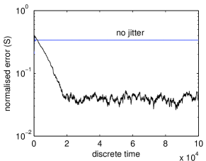
(a) Parameter $S$.

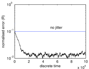
(b) Parameter $R$.

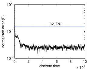
(c) Parameter $B$.

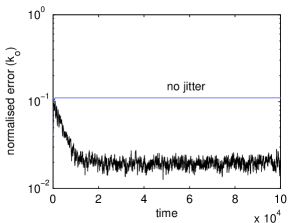
(d) Parameter $k_{o}$.

Figure 1: Average of the absolute parameter estimation errors over 50 independent simulation runs using Algorithm 3 with $N=M=300$ particles ($K=N^{2}=90\times 10^{3}$ particles overall). The absolute errors are normalised w.r.t. the true parameter values, $S=10,R=28,B=\frac{8}{3}$ and $k_{o}=\frac{4}{5}$. The results obtained when jittering is suppressed in Algorithm 3 (labeled as no jitter) are shown for comparison. The horizontal axis is in discrete-time units. As the integration period is ${\sf T}_{e}=10^{-3}$, $100,000$ discrete-time steps amount 100 continuous time units. Observations are collected every 40 discrete-time steps.

In Figure 2 we plot the average of the normalised errors versus the number of particles in Algorithm 3 (namely, for $N=150,300,600$). We have carried out 20 independent simulation trials (per point in the plot). In each simulation, the Lorenz system is run from continous time 0 to 24 (i.e., $24,000$ discrete time steps), with the errors computed by averaging $|\theta_{i,t}^{N,N}-\theta_{i}|/\theta_{i}$ over the continuous time interval (22,24). As in Figure 1, the performace of Algorithm 3 with the jittering step removed is also displayed, and again we observe how it fails to yield accurate parameter estimates. For the outputs of Algorithm 3 with jittering, we also display a least squares fit of the function $e(N)=\frac{c}{\sqrt{N}}$ to the averaged errors (with $c$ constant w.r.t. $N$), as suggested by Theorem 2.

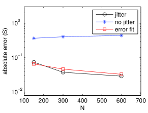
(a) Parameter $S$. The least squares fit of the errors yields $c\approx 0.807$.

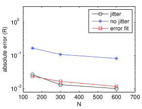
(b) Parameter $R$. The least squares fit of the errors yields $c\approx 0.290$.

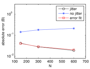
(c) Parameter $B$. The least squares fit of the errors yields $c\approx 0.496$.

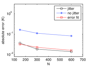
(d) Parameter $k_{o}$. The least squares fit of the errors yields $c\approx 0.397$.

Figure 2: Average of the absolute parameter estimation errors over 20 independent simulation runs using Algorithm 3 with $N=M=150$, $N=M=300$ and $N=M=600$ (the total number of particles is $N^{2}$). The errors are normalised w.r.t. the true parameter values, $S=10,R=28,B=\frac{8}{3}$ and $k_{o}=\frac{4}{5}$. The curves labeled error fit have the form $\frac{c}{\sqrt{N}}$, where the constant $c$ is a least squares estimate computed independently for each parameter. The results obtained when jittering is suppressed in Algorithm 3 (labeled as no jitter) are also shown for comparison. In each simulation, the Lorenz system was run for 24,000 discrete-time steps ($24$ continuous-time steps, for ${\sf T}_{e}=10^{-3}$), with observations collected every $40$ discrete steps.

Figure 3 displays the empirical variance for the average errors of Figure 2, with and without jittering. It shows that the variability of the estimators is relatively large for small $t$ and it reduces considerably as a longer observation record is accumulated.

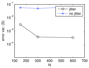
(a) Parameter $S$.

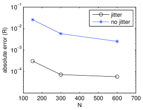
(b) Parameter $R$.

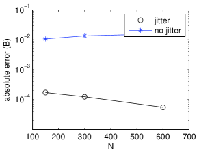
(c) Parameter $B$.

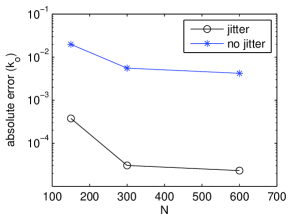
(d) Parameter $k_{o}$.

Figure 3: Empirical variance of the absolute parameter estimation errors over 20 independent simulation runs using Algorithm 3 with $N=M=150$, $N=M=300$ and $N=M=600$ (the total number of particles is $N^{2}$). The errors are normalised w.r.t. the true parameter values, $S=10,R=28,B=\frac{8}{3}$ and $k_{o}=\frac{4}{5}$. The results obtained when jittering is suppressed in Algorithm 3 (labeled as no jitter) are also shown for comparison. In each simulation, the Lorenz system was run for 24,000 discrete-time steps ($24$ continuous-time steps, for ${\sf T}_{e}=10^{-3}$), with observations collected every $40$ discrete steps.

Finally, we have carried out a simple computer experiment to test the effect of a change-point in one of the parameters (the observation scale factor $k_{o}$). The simulation setup is the same as in the rest of this Section except that we extend the support of the parameter $k_{o}$ to be the interval $\left[\frac{1}{2},8\right]$, with uniform a priori probability distribution, and artificially introduce a change-point at continuous time instant 30, where $k_{o}$ changes its value from $0.8$ to $5$. This change-point is not described by the model, that represents $k_{o}$ as strictly constant. We have run Algorithm 3 once, with $N=M=500$ particles, and observed the evolution over time of the posterior-mean estimators for $S$, $B$, $R$ and $k_{o}$.

Figure 4 shows that the posterior-mean estimates fluctuate considerably for (relatively) small $t$, as we concluded from observing their empirical variance. The value of $k_{o}$ is changed at discrete time $3\times 10^{4}$, which corresponds to continuous time 30 and a sequence of 750 observations. The change is instantaneous, yielding a step function for $k_{o}$ as plotted in Figure 4(d). Before the change-point, the random support of the posterior distribution of $k_{o}$ concentrates around the original value $k_{o}=0.8$. After the change-point, this support has to be adapted. However, the pace of this adaptation is limited by the variance of the jittering kernel and, hence, we observe a transition in the sequence of estimates that lasts for nearly $10^{4}$ time steps (10 continuous time units, 250 observations). Eventually, the posterior mean settles around the new value of $k_{o}$ in this simulation; however, further investigation is needed regarding the speed at which the random support of $\mu_{t}^{N,N}$ can be adapted and its interplay with estimation errors.

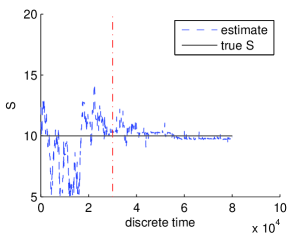
(a) Parameter $S$.

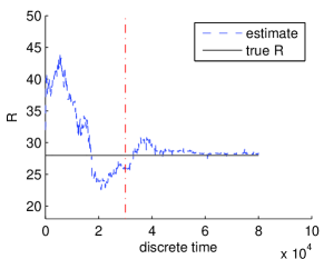
(b) Parameter $R$.

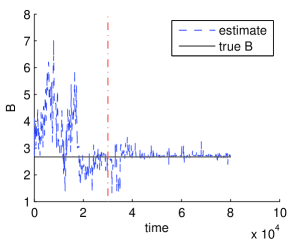
(c) Parameter $B$.

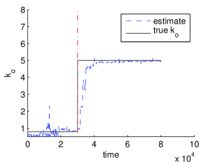
(d) Parameter $k_{o}$, with a change-point at time $3\times 10^{4}$.

Figure 4: Evolution over time of the posterior-mean estimates of the parameters $S$, $B$, $R$ and $k_{o}$ for a single run of Algorithm 3 with $N=M=500$. The actual parameter values of $S$, $R$, and $B$ are indicated with a horizontal solid line. The value of $k_{o}$ is also indicated, however it has a change-point at discrete time $3\times 10^{4}$ (from $0.8$ to 5). The change-point itself is marked by a vertical dashed line in the four plots. The algorithm is capable of tracking the change in $k_{o}$, however the adaptation of the estimator is limited by the variance of the jittering kernel and we observe a relatively long transition period of $\approx 10^{4}$ discrete time steps until the posterior mean settles around the new value.

7 Conclusions

We have introduced a recursive Monte Carlo scheme, consisting of two (nested) layers of particle filters, for the approximation and tracking of the posterior probability distribution of the unknown parameters of a state-space Markov system. Unlike existing SMC² and particle MCMC methods, the proposed algorithm is purely recursive and can be seen as a natural adaptation of the classic bootstrap filter to operate on the space of the static system-parameters.

The main theoretical contribution of the paper is the analysis of the errors in the approximation of integrals of bounded functions w.r.t. the posterior probability measure of the parameters. Using induction arguments, and placing only mild constraints on the state-space model and the parameters, we have proved that the $L_{p}$ norms of the approximation errors for the proposed algorithm vanish with rate proportional to $\frac{1}{\sqrt{N}}+\frac{1}{\sqrt{M}}$, where $N$ is the number of particles in the parameter space and $N\times M$ is the number of particles in the state space. This is achieved with a computational cost that grows only linearly with time. In comparison, the computational load of the SMC² method increases quadratically with time. The price to pay for this reduction in computational cost is that in the new scheme we need $N\rightarrow\infty$ and $M\rightarrow\infty$ in order to make the error converge towards 0, while the SMC² algorithm is consistent for fixed $M$, i.e., $N\rightarrow\infty$ is sufficient for the errors to vanish, independently of $M$. As a consequence, if $K=NM$ is the total number of particles in the state space, then the optimal allocation for the proposed nested particle filter is $N=M=\sqrt{K}$ and the errors converge as $K^{-\frac{1}{4}}$ in $L_{p}$, while the SMC² scheme, with $M$ fixed, converges as $K^{-\frac{1}{2}}$.

The proposed algorithm can be combined with a SMC² scheme for practical convenience. For example, one may run a standard SMC² algorithm on the initial part of the observation sequence (possibly a few tens or a few hundreds of observations, depending on the problem and the available computational resources) to take advantage of its faster convergence rate and then switch to a recursive nested particle filter (Algorithm 3) when the computational cost of batch processing becomes too high.

We also note that the continuity argument that leads to the derivation the the recursive nested particle filter, and the theoretical framework for the analysis of the resulting approximations, can be extended to other similar filtering algorithms. For example, it would be relatively straightforward to obtain a recursive version of the original IBIS algorithm of (Chopin, 2002).

Appendix A Proof of Lemma 1

We consider first the predictive measure

$$\xi_{t,\theta}^{N}(dx)=\frac{1}{N}\sum_{n=1}^{N}\delta_{\bar{x}_{t}^{(n)}}(dx)$$

where $\bar{x}_{t}^{(n)}$, $n=1,...,N$, are the state particles drawn from the transition kernels $\tau_{t,\theta}^{x_{t-1}^{(n)}}(dx)\triangleq\tau_{t,\theta}(dx|x_{t-1}^{(n)})$ at the sampling step of the particle filter. Recall that $\xi_{t,\theta}=\tau_{t,\theta}\phi_{t-1,\theta}$ and consider the triangle inequality

$$\left\|(f,\xi_{t,\theta}^{N})-(f,\xi_{t,\theta})\right\|_{p} = \left\|(f,\xi_{t,\theta}^{N})-(f,\tau_{t,\theta}\phi_{t-1,\theta})\right\|_{p}$$ (A.1)

$$\leq \left\|(f,\xi_{t,\theta}^{N})-(f,\tau_{t,\theta}\phi_{t-1,\theta}^{N})\right\|_{p}$$

$$+\left\|(f,\tau_{t,\theta}\phi_{t-1,\theta}^{N})-(f,\tau_{t,\theta}\phi_{t-1,\theta})\right\|_{p},$$

where

$$(f,\tau_{t,\theta}\phi_{t-1,\theta}^{N})=\frac{1}{N}\sum_{n=1}^{N}\int f(x)\tau_{t,\theta}(dx|x_{t-1}^{(n)})=\frac{1}{N}\sum_{n=1}^{N}(f,\tau_{t,\theta}^{x_{t-1}^{(n)}}).$$ (A.2)

In the sequel we seek upper bounds for the $L_{p}$ norms in the right hand side of (A.1).

Let us introduce the $\sigma$-algebra generated by the random paths $x_{0:t}^{(n)}$ and $\bar{x}_{1:t}^{(n)}$, $n=1,...,N$, denoted ${\mathcal{F}}_{t}=\sigma\left(x_{0:t}^{(n)},\bar{x}_{1:t}^{(n)},\quad n=1,...,N\right)$. The conditional expectation of the integral $(f,\xi_{t,\theta}^{N})$ given ${\mathcal{F}}_{t-1}$ is

$$E\left[(f,\xi_{t,\theta}^{N})|{\mathcal{F}}_{t-1}\right] = \frac{1}{N}\sum_{n=1}^{N}E\left[f(\bar{x}_{t}^{(n)})|{\mathcal{F}}_{t-1}\right]$$

$$= \frac{1}{N}\sum_{n=1}^{N}(f,\tau_{t,\theta}^{x_{t-1}^{(n)}})=(f,\tau_{t,\theta}\phi_{t-1,\theta}^{N})$$

and we note that the random variables $S_{t,\theta}^{(n)}=f(\bar{x}_{t}^{(n)})-(f,\tau_{t,\theta}^{x_{t-1}^{(n)}})$, $n=1,...,N$, are independent and zero-mean conditional on the $\sigma$-algebra ${\mathcal{F}}_{t-1}$. For even $p$, the approximation error between $\xi_{t,\theta}^{N}$ and its (conditional) expected value $\tau_{t,\theta}\phi_{t-1,\theta}^{N}$ can then be written as

$$E\left[\left((f,\xi_{t,\theta}^{N})-(f,\tau_{t}\phi_{t-1,\theta}^{N})\right)^{p}|{\mathcal{F}}_{t-1}\right] = E\left[\left(\frac{1}{N}\sum_{n=1}^{N}S_{t,\theta}^{(n)}\right)^{p}|{\mathcal{F}}_{t-1}\right]$$

$$= \frac{1}{N^{p}}\sum_{n_{1}=1}^{N}\cdots\sum_{n_{p}=1}^{N}E\left[S_{t,\theta}^{(n_{1})}\ldots S_{t,\theta}^{(n_{p})}|{\mathcal{F}}_{t-1}\right].$$

Since the random variables $S_{t,\theta}^{(n_{i})}$ are conditionally independent and zero-mean, every term in the summation of (LABEL:eqCombinations) involving a moment of order 1 vanishes. It is an exercise in combinatorics to show that the number of terms which do not contain any moment of order 1 is a polynomial function of $N$ with degree $\frac{p}{2}$, whose coefficients depend only on $p$. As a consequence, there exists a constant $\tilde{c}$ independent of $N$ such that the number of non-zero terms in (LABEL:eqCombinations) is at most $\tilde{c}^{p}N^{\frac{p}{2}}$. Moreover, for each non-zero term we readily calculate the upper bound $E\left[S_{t,\theta}^{(n_{1})}\ldots S_{t,\theta}^{(n_{p})}|{\mathcal{F}}_{t-1}\right]\leq 2^{p}\|f\|_{\infty}^{p}$. Therefore, for even $p$, we arrive at the inequality

$$E\left[\left((f,\xi_{t,\theta}^{N})-(f,\tau_{t}\phi_{t-1,\theta}^{N})\right)^{p}|{\mathcal{F}}_{t-1}\right]\leq\frac{\tilde{c}^{p}2^{p}\|f\|_{\infty}^{p}}{N^{\frac{p}{2}}}$$ (A.4)

and taking unconditional expectations on both sides of (A.4), we readily find that,

$$\|(f,\xi_{t,\theta}^{N})-(f,\tau_{t}\phi_{t-1,\theta}^{N}\|_{p}\leq\frac{c_{1}\|f\|_{\infty}}{\sqrt{N}},$$ (A.5)

where $c_{1}=2\tilde{c}$ is a constant independent of $N$ and $\theta$. The same inequality (A.5) holds for any real $p$ because of the monotonicity of $L_{p}$ norms (an application of Jensen’s inequality).

For the second term in the right hand side of (A.1), we note that $(f,\tau_{t,\theta}\phi_{t-1,\theta})=(\bar{f}_{\theta},\phi_{t-1,\theta})$, where $\bar{f}_{\theta}\in B(\mathbb{R}^{d_{x}})$ is a bounded function defined as

$$\bar{f}_{\theta}(x)=\int f(x^{\prime})\tau_{t,\theta}^{x}(dx^{\prime})=(f,\tau_{t,\theta}^{x})$$

and, similarly, $(f,\tau_{t,\theta}\phi_{t-1,\theta}^{N})=(\bar{f}_{\theta},\phi_{t-1,\theta}^{N})$. Therefore, assumption (2.15) yields the upper bound

$$\left\|(f,\tau_{t,\theta}\phi_{t-1,\theta}^{N})-(f,\tau_{t,\theta}\phi_{t-1,\theta})\right\|_{p} = \left\|(\bar{f}_{\theta},\phi_{t-1,\theta}^{N})-(\bar{f}_{\theta},\phi_{t-1,\theta})\right\|_{p}Ê$$ (A.6)

$$\leq \frac{c_{t-1}\|f\|_{\infty}}{\sqrt{N}}+\frac{\bar{c}_{t-1}\|f\|_{\infty}}{\sqrt{M}},$$

where the constants $c_{t-1},\bar{c}_{t-1}$ are independent of $N$, $M$ and $\theta$. Substituting (A.5) and (A.6) into (A.1) yields

$$\left\|(f,\xi_{t,\theta}^{N})-(f,\xi_{t,\theta})\right\|_{p} \leq \frac{\tilde{c}_{t}\|f\|_{\infty}}{\sqrt{N}}+\frac{\bar{\tilde{c}}_{t}\|f\|_{\infty}}{\sqrt{M}},$$ (A.7)

where $\tilde{c}_{t}=c_{t-1}+c_{1}$ and $\bar{\tilde{c}}_{t}=\bar{c}_{t-1}$ are finite constants independent of $N$, $M$ and $\theta$.

Next, we use inequality (A.7) to calculate a bound on $\|(f,\phi_{t,\theta}^{N})-(f,\phi_{t,\theta})\|_{p}$. Let us first note that, after the computation of the weights, we obtain a random measure of the form

$$\bar{\phi}_{t,\theta}^{N}(dx)=\sum_{n=1}^{N}w_{t}^{(n)}\delta_{\bar{x}_{t}^{(n)}}(dx),\quad\mbox{where}\quad w_{t}^{(n)}=\frac{g_{t,\theta}^{y_{t}}(\bar{x}_{t}^{(n)})}{\sum_{k=1}^{N}g_{t,\theta}^{y_{t}}(\bar{x}_{t}^{(n)})}.$$

As a consequence, integrals w.r.t. the measure $\bar{\phi}_{t,\theta}^{N}$ can be written in terms of $g_{t,\theta}^{y_{t}}$ and $\xi_{t,\theta}^{N}$, namely

$$(f,\bar{\phi}_{t,\theta}^{N})=\frac{(fg_{t,\theta}^{y_{t}},\xi_{t,\theta}^{N})}{(g_{t,\theta}^{y_{t}},\xi_{t,\theta}^{N})}.$$ (A.8)

This is natural, though, since from the Bayes theorem we readily derive the same relationship between $\phi_{t,\theta}$ and $\xi_{t,\theta}$,

$$(f,\phi_{t,\theta})=\frac{(fg_{t,\theta}^{y_{t}},\xi_{t,\theta})}{(g_{t,\theta}^{y_{t}},\xi_{t,\theta})}.$$ (A.9)

Given (A.8) and (A.9), we can readily apply the inequality (2.1) to obtain

$$\left|(f,\bar{\phi}_{t,\theta}^{N})-(f,\phi_{t,\theta})\right| \leq \frac{1}{(g_{t,\theta}^{y_{t,\theta}},\xi_{t,\theta})}\left(\|f\|_{\infty}\left|(g_{t,\theta}^{y_{t}},\xi_{t,\theta})-(g_{t,\theta},\xi_{t,\theta}^{N})\right|\right.$$ (A.10)

$$\left.+\left|(fg_{t,\theta}^{y_{t}},\xi_{t,\theta})-(fg_{t,\theta},\xi_{t,\theta}^{N})\right|\right),$$

where $u_{t}(\theta)=(g_{t,\theta}^{y_{t,\theta}},\xi_{t,\theta})>0$ by assumption. From (A.10) and Minkowski’s inequality,

$$\left\|(f,\bar{\phi}_{t,\theta}^{N})-(f,\phi_{t,\theta})\right\|_{p} \leq \frac{1}{(g_{t,\theta}^{y_{t,\theta}},\xi_{t,\theta})}\times\left(\|f\|_{\infty}\left\|(g_{t,\theta}^{y_{t}},\xi_{t,\theta})-(g_{t,\theta}^{y_{t}},\xi_{t,\theta}^{N})\right\|_{p}\right.$$ (A.11)

$$\left.+\left\|(fg_{t,\theta}^{y_{t}},\xi_{t,\theta})-(fg_{t,\theta},\xi_{t,\theta}^{N})\right\|_{p}\right)$$

and, since $\|g_{t,\theta}^{y_{t}}\|_{\infty}\leq\|g_{t}^{y_{t}}\|_{\infty}<\infty$ by assumption (in particular, $\|g_{t}^{y_{t}}\|_{\infty}$ is independent of $\theta$), the inequalities (A.7) and (A.11) together yield

$$\left\|(f,\bar{\phi}_{t,\theta}^{N})-(f,\phi_{t,\theta})\right\|_{p}\leq\frac{2\|f\|_{\infty}\|g_{t}^{y_{t}}\|_{\infty}\tilde{c}_{t}}{(g_{t,\theta}^{y_{t,\theta}},\xi_{t,\theta})}\times\frac{1}{\sqrt{N}}+\frac{2\|f\|_{\infty}\|g_{t}^{y_{t}}\|_{\infty}\bar{\tilde{c}}_{t}}{(g_{t,\theta}^{y_{t,\theta}},\xi_{t,\theta})}\times\frac{1}{\sqrt{M}},$$ (A.12)

where the finite constants $\tilde{c}_{t}$ and $\bar{\tilde{c}}_{t}=\bar{c}_{t-1}$ are independent of $N$, $M$ and $\theta$. Indeed, the only factor that depends on $\theta$ in the right-hand side of (A.12) is the integral $u_{t}(\theta)=(g_{t,\theta}^{y_{t,\theta}},\xi_{t,\theta})$. However, we have assumed that

$$u_{t,\inf}=\inf_{\theta\in D_{\theta}}u_{t}(\theta)>0,$$ (A.13)

hence the inequality (A.12) leads to

$$\left\|(f,\bar{\phi}_{t,\theta}^{N})-(f,\phi_{t,\theta})\right\|_{p}\leq\frac{c_{2,t}\|f\|_{\infty}}{\sqrt{N}}+\frac{\bar{c}_{2,t}\|f\|_{\infty}}{\sqrt{M}}$$ (A.14)

where

$$c_{2,t}=\frac{2\|g_{t}^{y_{t}}\|_{\infty}\tilde{c}_{t}}{u_{t,\inf}}<\infty\quad\mbox{and}\quad\bar{c}_{2,t}=\frac{2\|g_{t}^{y_{t}}\|_{\infty}\bar{c}_{t-1}}{u_{t,\inf}}<\infty$$ (A.15)

are constants independent of $N$, $M$ and $\theta$.

Finally, we only need to verify the resampling step, i.e., that the $L_{p}$ norm $\|(f,\phi_{t,\theta}^{N})-(f,\bar{\phi}_{t,\theta}^{N})\|_{p}$ is bounded as well. Let $\bar{\mathcal{F}}_{t}=\sigma\left(x_{0:t-1}^{(n)},\bar{x}_{1:t}^{(n)};n=1,\ldots,N\right)$ be the $\sigma$-algebra generated by the random sequences $x_{0:t-1}^{(n)}$ and $\bar{x}_{1:t}^{(n)}$, $n=1,...,N$. It is straightforward to check that, for every $n=1,...,N$,

$$E\left[f(x_{t}^{(n)})|\bar{\mathcal{F}}_{t}\right]=(f,\bar{\phi}_{t,\theta}^{N}),$$ (A.16)

hence the random variables $\bar{S}_{t,\theta}^{(n)}=f(x_{t}^{(n)})-(f,\bar{\phi}_{t,\theta}^{N})$ are independent and zero-mean conditional on the $\sigma$-algebra $\bar{\mathcal{F}}_{t}$. Therefore, the same combinatorial argument that led to Eq. (A.5) now yields

$$\left\|(f,\phi_{t,\theta}^{N})-(f,\bar{\phi}_{t,\theta}^{N})\right\|_{p}\leq\frac{c_{3}\|f\|_{\infty}}{\sqrt{N}}$$ (A.17)

where the constant $c_{3}$ is independent of both $N$ and $\theta$ (it does not depend on the distribution of the error variables $\bar{S}_{t,\theta}^{(n)}$). Since

$$\|(f,\phi_{t,\theta}^{N})-(f,\phi_{t,\theta})\|_{p}\leq\|(f,\phi_{t,\theta}^{N})-(f,\bar{\phi}_{t,\theta}^{N})\|_{p}+\|(f,\bar{\phi}_{t,\theta}^{N})-(f,\phi_{t,\theta})\|_{p},$$ (A.18)

substituting Eqs. (A.17) and (A.14) into the inequality (A.18) yields

$$\|(f,\phi_{t,\theta}^{N})-(f,\phi_{t,\theta})\|_{p}\leq\frac{c_{t}\|f\|_{\infty}}{\sqrt{N}}+\frac{\bar{c}_{t}\|f\|_{\infty}}{\sqrt{M}},$$ (A.19)

where $c_{t}=c_{3}+c_{2,t}$ and $\bar{c}_{t}=\bar{c}_{2,t}$ are finite constants independent of both $N$, $M$ and $\theta$.

To complete the proof, simply note that $\bar{c}_{t-1}=0$ implies $\bar{c}_{t}=\bar{c}_{2,t}=0$ (see (A.15)). $\Box$

Appendix B Proof of Lemma 2

We proceed by induction in $t$. For $t=0$, the measure $\phi_{0,\theta}^{N}(dx)=\frac{1}{N}\sum_{n=1}^{N}\delta_{x_{0}^{(n)}}(dx)$ is constructed from an i.i.d. sample of size $N$ from the prior distribution $\phi_{0,\theta}\equiv\tau_{0}$. Then, it is straightforward to prove that

$$\|(f,\phi_{0,\theta}^{N})-(f,\phi_{0,\theta})\|_{p}\leq\frac{c_{0}\|f\|_{\infty}}{\sqrt{N}},$$

where $c_{0}<\infty$ is independent of $N$. Note that, since $\phi_{0,\theta}\equiv\tau_{0}$ is actually independent of $\theta$, the constant $c_{0}$ is independent of $\theta$ as well.

For the induction step, we assume that

$$\|(f,\phi_{t-1,\theta}^{N})-(f,\phi_{t-1,\theta})\|_{p}\leq\frac{c_{t-1}\|f\|_{\infty}}{\sqrt{N}}$$ (B.1)

holds true for some constant $c_{t-1}<\infty$ independent of $N$ and $\theta$. Given (B.1), Lemma 1 yields

$$\|(f,\xi_{t,\theta}^{N})-(f,\xi_{t,\theta})\|_{p}\leq\frac{\tilde{c}_{t}\|f\|_{\infty}}{\sqrt{N}}\quad\mbox{and}\quad\|(f,\phi_{t,\theta}^{N})-(f,\phi_{t,\theta})\|_{p}\leq\frac{c_{t}\|f\|_{\infty}}{\sqrt{N}}$$

at time $t$, where $\tilde{c}_{t}$ and $c_{t}$ are finite constants independent of $N$ and $\theta$. $\Box$

Appendix C A family of jittering kernels

Proposition 1.

Assume that $h\in B(D_{\theta})$ is Lipschitz, with constant $c_{L}\|h\|_{\infty}<\infty$, and consider the class of kernels $\kappa_{N}^{\theta^{\prime}}=(1-\epsilon_{N})\delta_{\theta^{\prime}}+\epsilon_{N}\bar{\kappa}_{N}^{\theta^{\prime}}$, where $0\leq\epsilon_{N}\leq 1$ and $\bar{\kappa}_{N}^{\theta^{\prime}}\in{\mathcal{P}}(D_{\theta})$. For any $p\geq 1$, if the kernel $\kappa_{N}^{\theta^{\prime}}$ is selected in such a way that

$$\sigma_{\kappa,N}^{2}=\sup_{\theta^{\prime}\in D_{\theta}}\int\|\theta-\theta^{\prime}\|^{2}\bar{\kappa}_{N}^{\theta^{\prime}}(d\theta)\leq\frac{\breve{c}}{\epsilon_{N}^{\frac{p+2}{p}}N^{\frac{p+2}{2}}}$$ (C.1)

is satisfied for some constant $\breve{c}<\infty$ independent of $N$, then the inequality

$$\sup_{\theta^{\prime}\in D_{\theta}}\int|h(\theta)-h(\theta^{\prime})|^{p}\kappa_{N}^{\theta^{\prime}}(d\theta)\leq\frac{c_{\kappa}^{p}\|h\|_{\infty}^{p}}{N^{\frac{p}{2}}}$$

holds for a constant $c_{\kappa}^{p}=c_{L}^{p}\left(1+\breve{c}\sup_{\theta_{1},\theta_{2}\in D_{\theta}}\|\theta_{1}-\theta_{2}\|^{p}\right)<\infty$ independent of $N$.

Proof. Since $\kappa_{N}^{\theta^{\prime}}=(1-\epsilon_{N})\delta_{\theta^{\prime}}+\epsilon_{N}\bar{\kappa}_{N}^{\theta^{\prime}}$ and $h$ is Lipschitz with constant $c_{L}\|h\|_{\infty}<\infty$, we readily obtain

$$\int|h(\theta)-h(\theta^{\prime})|^{p}\kappa_{N}^{\theta^{\prime}}(d\theta)\leq\epsilon_{N}c_{L}^{p}\|h\|_{\infty}^{p}\int\|\theta-\theta^{\prime}\|^{p}\bar{\kappa}_{N}^{\theta^{\prime}}(d\theta).$$ (C.2)

Let

$$\beta_{N}=\frac{1}{\epsilon_{N}^{\frac{1}{p}}\sqrt{N}}.$$ (C.3)

We can rewrite (C.2) as

$$\int|h(\theta)-h(\theta^{\prime})|^{p}\kappa_{N}^{\theta^{\prime}}(d\theta) \leq \epsilon_{N}c_{L}^{p}\|h\|_{\infty}^{p}\left[\int I_{\theta\in D_{\theta}:\|\theta-\theta^{\prime}\|<\beta_{N}}(\theta)\|\theta-\theta^{\prime}\|^{p}\bar{\kappa}_{N}^{\theta^{\prime}}(d\theta)\right.$$

$$\left.+\int I_{\theta\in D_{\theta}:\|\theta-\theta^{\prime}\|\geq\beta_{N}}(\theta)\|\theta-\theta^{\prime}\|^{p}\bar{\kappa}_{N}^{\theta^{\prime}}(d\theta)\right]$$

$$\leq \epsilon_{N}c_{L}^{p}\|h\|_{\infty}^{p}\left[\beta_{N}^{p}+\hat{C}^{p}\int I_{\theta\in D_{\theta}:\|\theta-\theta^{\prime}\|\geq\beta_{N}}(\theta)\bar{\kappa}_{N}^{\theta^{\prime}}(d\theta)\right],$$

where $\hat{C}^{p}=\sup_{\theta_{1},\theta_{2}\in D_{\theta}}\|\theta_{1}-\theta_{2}\|^{p}<\infty$, since $D_{\theta}$ is compact. Using Chebyshev’s inequality on the right hand side of (LABEL:eqPeque2) yields

$$\int|h(\theta)-h(\theta^{\prime})|^{p}\kappa_{N}^{\theta^{\prime}}(d\theta)\leq\epsilon_{N}c_{L}^{p}\|h\|_{\infty}^{p}\left(\beta_{N}^{p}+\hat{C}^{p}\frac{\sigma_{\kappa,N}^{2}}{\beta_{N}^{2}}\right)$$ (C.5)

and substituting (C.1) and (C.3) into (C.5) we arrive at

$$\int|h(\theta)-h(\theta^{\prime})|^{p}\kappa_{N}^{\theta^{\prime}}(d\theta)\leq\frac{c_{L}^{p}\|h\|_{\infty}^{p}\left(1+\breve{c}\hat{C}^{p}\right)}{N^{\frac{p}{2}}},$$

where all the constants are independent of $\theta^{\prime}$ and $N$. $\Box$

Corollary 1.

Consider the same class of kernels $\kappa_{N}^{\theta^{\prime}}=(1-\epsilon_{N})\delta_{\theta^{\prime}}+\epsilon_{N}\bar{\kappa}_{N}^{\theta^{\prime}}$, where $0\leq\epsilon_{N}\leq 1$ and $\bar{\kappa}_{N}^{\theta^{\prime}}\in{\mathcal{P}}(D_{\theta})$. For any $p\geq 1$, if (C.1) holds for some $\breve{c}<\infty$ independent of $N$ then

$$\sup_{\theta^{\prime}\in D_{\theta}}\int\|\theta-\theta^{\prime}\|^{p}\kappa_{N}^{\theta^{\prime}}(d\theta)\leq\frac{c_{\kappa}^{p}}{N^{\frac{p}{2}}}$$

where $c_{\kappa}^{p}=1+\breve{c}\sup_{\theta_{1},\theta_{2}\in D_{\theta}}\|\theta_{1}-\theta_{2}\|^{p}<\infty$ is constant and independent of $N$.

Proof. Simply note that

$$\int\|\theta-\theta^{\prime}\|^{p}\kappa_{N}^{\theta^{\prime}}(d\theta)\leq\epsilon_{N}\int\|\theta-\theta^{\prime}\|^{p}\bar{\kappa}_{N}^{\theta^{\prime}}(d\theta)$$

and then follow the same argument as in the proof of Proposition 1. $\Box$

References

• Andrieu, Doucet and Holenstein (2010) {barticle}[author] \bauthor\bsnmAndrieu, \bfnmC.\binitsC., \bauthor\bsnmDoucet, \bfnmA.\binitsA. and \bauthor\bsnmHolenstein, \bfnmR.\binitsR. (\byear2010). \btitleParticle Markov chain Monte Carlo methods. \bjournalJournal of the Royal Statistical Society B \bvolume72 \bpages269–342. \endbibitem
• Andrieu et al. (2004) {barticle}[author] \bauthor\bsnmAndrieu, \bfnmC.\binitsC., \bauthor\bsnmDoucet, \bfnmA.\binitsA., \bauthor\bsnmSingh, \bfnmS. S.\binitsS. S. and \bauthor\bsnmTadić, \bfnmV. B.\binitsV. B. (\byear2004). \btitleParticle Methods for Change Detection, System Identification and Control. \bjournalProceedings of the IEEE \bvolume92 \bpages423-438. \endbibitem
• Beskos et al. (2014) {barticle}[author] \bauthor\bsnmBeskos, \bfnmAlexandros\binitsA., \bauthor\bsnmCrisan, \bfnmDan\binitsD., \bauthor\bsnmJasra, \bfnmAjay\binitsA. \betalet al. (\byear2014). \btitleOn the stability of sequential Monte Carlo methods in high dimensions. \bjournalThe Annals of Applied Probability \bvolume24 \bpages1396–1445. \endbibitem
• Bruno (2013) {barticle}[author] \bauthor\bsnmBruno, \bfnmM. G. S.\binitsM. G. S. (\byear2013). \btitleSequential Monte Carlo Methods for Nonlinear Discrete-Time Filtering. \bjournalSynthesis Lectures on Signal Processing \bvolume6 \bpages1–99. \endbibitem
• Cappé, Godsill and Moulines (2007) {barticle}[author] \bauthor\bsnmCappé, \bfnmO.\binitsO., \bauthor\bsnmGodsill, \bfnmS. J.\binitsS. J. and \bauthor\bsnmMoulines, \bfnmE.\binitsE. (\byear2007). \btitleAn overview of existing methods and recent advances in sequential Monte Carlo. \bjournalProceedings of the IEEE \bvolume95 \bpages899–924. \endbibitem
• Cappé et al. (2004) {barticle}[author] \bauthor\bsnmCappé, \bfnmO.\binitsO., \bauthor\bsnmGullin, \bfnmA.\binitsA., \bauthor\bsnmMarin, \bfnmJ. M.\binitsJ. M. and \bauthor\bsnmRobert, \bfnmC. P.\binitsC. P. (\byear2004). \btitlePopulation Monte Carlo. \bjournalJournal of Computational and Graphical Statistics \bvolume13 \bpages907-929. \endbibitem
• Carvalho et al. (2010) {barticle}[author] \bauthor\bsnmCarvalho, \bfnmC. M.\binitsC. M., \bauthor\bsnmJohannes, \bfnmM. S.\binitsM. S., \bauthor\bsnmLopes, \bfnmH. F.\binitsH. F. and \bauthor\bsnmPolson, \bfnmN. G.\binitsN. G. (\byear2010). \btitleParticle learning and smoothing. \bjournalStatistical Science \bvolume25 \bpages88–106. \endbibitem
• Chen, Wang and Liu (2000) {barticle}[author] \bauthor\bsnmChen, \bfnmR.\binitsR., \bauthor\bsnmWang, \bfnmX.\binitsX. and \bauthor\bsnmLiu, \bfnmJ. S.\binitsJ. S. (\byear2000). \btitleAdaptive Joint Detection and Decoding in Flat-Fading Channels via Mixture Kalman Filtering. \bjournalIEEE Transactions Information Theory \bvolume46 \bpages2079-2094. \endbibitem
• Chopin (2002) {barticle}[author] \bauthor\bsnmChopin, \bfnmN.\binitsN. (\byear2002). \btitleA sequential particle filter method for static models. \bjournalBiometrika \bvolume89 \bpages539–552. \endbibitem
• Chopin, Jacob and Papaspiliopoulos (2013) {barticle}[author] \bauthor\bsnmChopin, \bfnmN.\binitsN., \bauthor\bsnmJacob, \bfnmP. E.\binitsP. E. and \bauthor\bsnmPapaspiliopoulos, \bfnmO.\binitsO. (\byear2013). \btitleSMC2: an efficient algorithm for sequential analysis of state space models. \bjournalJournal of the Royal Statistical Society: Series B (Statistical Methodology) \bvolume75 \bpages397–426. \endbibitem
• Chorin and Krause (2004) {barticle}[author] \bauthor\bsnmChorin, \bfnmA. J.\binitsA. J. and \bauthor\bsnmKrause, \bfnmP.\binitsP. (\byear2004). \btitleDimensional Reduction for a Bayesian Filter. \bjournalPNAS \bvolume101 \bpages15013-15017. \endbibitem
• Crisan (2001) {bincollection}[author] \bauthor\bsnmCrisan, \bfnmD.\binitsD. (\byear2001). \btitleParticle Filters - A Theoretical Perspective. In \bbooktitleSequential Monte Carlo Methods in Practice (\beditor\bfnmA.\binitsA. \bsnmDoucet, \beditor\bfnmN.\binitsN. \bparticlede \bsnmFreitas and \beditor\bfnmN.\binitsN. \bsnmGordon, eds.) \bchapter2, \bpages17-42. \bpublisherSpringer. \endbibitem
• Crisan and Doucet (2002) {barticle}[author] \bauthor\bsnmCrisan, \bfnmD.\binitsD. and \bauthor\bsnmDoucet, \bfnmA.\binitsA. (\byear2002). \btitleA Survey of Convergence Results on Particle Filtering. \bjournalIEEE Transactions Signal Processing \bvolume50 \bpages736-746. \endbibitem
• Douc, Cappé and Moulines (2005) {binproceedings}[author] \bauthor\bsnmDouc, \bfnmR.\binitsR., \bauthor\bsnmCappé, \bfnmO.\binitsO. and \bauthor\bsnmMoulines, \bfnmE.\binitsE. (\byear2005). \btitleComparison of Resampling Schemes for Particle Filtering. In \bbooktitleProceedings of the 4th International Symposium on Image and Signal Processing and Analysis \bpages64-69. \endbibitem
• Doucet, de Freitas and Gordon (2001) {bincollection}[author] \bauthor\bsnmDoucet, \bfnmA.\binitsA., \bauthor\bparticlede \bsnmFreitas, \bfnmN.\binitsN. and \bauthor\bsnmGordon, \bfnmN.\binitsN. (\byear2001). \btitleAn introduction to sequential Monte Carlo methods. In \bbooktitleSequential Monte Carlo Methods in Practice (\beditor\bfnmA.\binitsA. \bsnmDoucet, \beditor\bfnmN.\binitsN. \bparticlede \bsnmFreitas and \beditor\bfnmN.\binitsN. \bsnmGordon, eds.) \bchapter1, \bpages4-14. \bpublisherSpringer. \endbibitem
• Doucet, Godsill and Andrieu (2000) {barticle}[author] \bauthor\bsnmDoucet, \bfnmA.\binitsA., \bauthor\bsnmGodsill, \bfnmS.\binitsS. and \bauthor\bsnmAndrieu, \bfnmC.\binitsC. (\byear2000). \btitleOn sequential Monte Carlo Sampling methods for Bayesian filtering. \bjournalStatistics and Computing \bvolume10 \bpages197-208. \endbibitem
• Fearnhead (2002) {barticle}[author] \bauthor\bsnmFearnhead, \bfnmP.\binitsP. (\byear2002). \btitleMarkov chain Monte Carlo, sufficient statistics, and particle filters. \bjournalJournal of Computational and Graphical Statistics \bvolume11 \bpages848–862. \endbibitem
• Gilks and Berzuini (2001) {barticle}[author] \bauthor\bsnmGilks, \bfnmW. R.\binitsW. R. and \bauthor\bsnmBerzuini, \bfnmC.\binitsC. (\byear2001). \btitleFollowing a moving targetÑMonte Carlo inference for dynamic Bayesian models. \bjournalJournal of the Royal Statistical Society: Series B (Statistical Methodology) \bvolume63 \bpages127–146. \endbibitem
• Gordon, Salmond and Smith (1993) {barticle}[author] \bauthor\bsnmGordon, \bfnmN.\binitsN., \bauthor\bsnmSalmond, \bfnmD.\binitsD. and \bauthor\bsnmSmith, \bfnmA. F. M.\binitsA. F. M. (\byear1993). \btitleNovel Approach to Nonlinear and Non-Gaussian Bayesian State Estimation. \bjournalIEE Proceedings-F \bvolume140 \bpages107-113. \endbibitem
• Kantas et al. (2015) {barticle}[author] \bauthor\bsnmKantas, \bfnmN.\binitsN., \bauthor\bsnmDoucet, \bfnmA.\binitsA., \bauthor\bsnmSingh, \bfnmS. S.\binitsS. S., \bauthor\bsnmMaciejowski, \bfnmJ. M.\binitsJ. M. and \bauthor\bsnmChopin, \bfnmN.\binitsN. (\byear2015). \btitleOn Particle Methods for Parameter Estimation in State-Space Models. \bjournalStatistical Science \bvolume30 \bpages328-351. \endbibitem
• Kitagawa (1996) {barticle}[author] \bauthor\bsnmKitagawa, \bfnmG.\binitsG. (\byear1996). \btitleMonte Carlo filter and smoother for non-Gaussian nonlinear state-space models. \bjournalJ. Comput. Graph. Statist. \bvolume1 \bpages1-25. \endbibitem
• Kitagawa (1998) {barticle}[author] \bauthor\bsnmKitagawa, \bfnmG.\binitsG. (\byear1998). \btitleA self-organizing state-space model. \bjournalJournal of the American Statistical Association \bpages1203–1215. \endbibitem
• Koblents and Míguez (2013) {barticle}[author] \bauthor\bsnmKoblents, \bfnmE.\binitsE. and \bauthor\bsnmMíguez, \bfnmJ.\binitsJ. (\byear2013). \btitleA population Monte Carlo scheme with transformed weights and its application to stochastic kinetic models. \bjournalStatistics and Computing. \bdoi10.1007/s11222-013-9440-2 \endbibitem
• Koblents and Míguez (2015) {barticle}[author] \bauthor\bsnmKoblents, \bfnmE.\binitsE. and \bauthor\bsnmMíguez, \bfnmJ.\binitsJ. (\byear2015). \btitleA population Monte Carlo scheme with transformed weights and its application to stochastic kinetic models. \bjournalStatistics and Computing \bvolume25 \bpages407–425. \endbibitem
• Kong, Liu and Wong (1994) {barticle}[author] \bauthor\bsnmKong, \bfnmA.\binitsA., \bauthor\bsnmLiu, \bfnmJ. S.\binitsJ. S. and \bauthor\bsnmWong, \bfnmW. H.\binitsW. H. (\byear1994). \btitleSequential imputations and Bayesian missing data problems. \bjournalJournal of the American Statistical Association \bvolume9 \bpages278-288. \endbibitem
• LeGland and Mevel (1997) {binproceedings}[author] \bauthor\bsnmLeGland, \bfnmF.\binitsF. and \bauthor\bsnmMevel, \bfnmL.\binitsL. (\byear1997). \btitleRecursive estimation in hidden Markov models. In \bbooktitleProceedings of the 36th IEEE Conference on Decision and Control, 1997 \bvolume4 \bpages3468–3473. \bpublisherIEEE. \endbibitem
• Liu and Chen (1998) {barticle}[author] \bauthor\bsnmLiu, \bfnmJ. S.\binitsJ. S. and \bauthor\bsnmChen, \bfnmR.\binitsR. (\byear1998). \btitleSequential Monte Carlo Methods for Dynamic Systems. \bjournalJournal of the American Statistical Association \bvolume93 \bpages1032-1044. \endbibitem
• Liu and West (2001) {bincollection}[author] \bauthor\bsnmLiu, \bfnmJ.\binitsJ. and \bauthor\bsnmWest, \bfnmM.\binitsM. (\byear2001). \btitleCombined parameter and state estimation in simulation-based filtering. In \bbooktitleSequential Monte Carlo Methods in Practice (\beditor\bfnmA.\binitsA. \bsnmDoucet, \beditor\bfnmN.\binitsN. \bparticlede \bsnmFreitas and \beditor\bfnmN.\binitsN. \bsnmGordon, eds.) \bchapter10, \bpages197-223. \bpublisherSpringer. \endbibitem
• Lorenz (1963) {barticle}[author] \bauthor\bsnmLorenz, \bfnmE. N.\binitsE. N. (\byear1963). \btitleDeterministic Nonperiodic Flow. \bjournalJournal of Atmospheric Sciences \bvolume20 \bpages130-141. \endbibitem
• Maíz et al. (2012) {barticle}[author] \bauthor\bsnmMaíz, \bfnmC. S.\binitsC. S., \bauthor\bsnmMolanes-López, \bfnmE.\binitsE., \bauthor\bsnmMíguez, \bfnmJ.\binitsJ. and \bauthor\bsnmDjurić, \bfnmP. M.\binitsP. M. (\byear2012). \btitleA Particle Filtering Scheme for Processing Time Series Corrupted by Outliers. \bjournalIEEE Transactions on Signal Processing \bvolume9. \endbibitem
• Miguez, Bugallo and Djuric (2005) {binproceedings}[author] \bauthor\bsnmMiguez, \bfnmJ.\binitsJ., \bauthor\bsnmBugallo, \bfnmM.\binitsM. and \bauthor\bsnmDjuric, \bfnmP. M.\binitsP. M. (\byear2005). \btitleNovel particle filtering algorithms for fixed parameter estimation in dynamic systems. In \bbooktitleProceedings of the 4th International Symposium on Image and Signal Processing and Analysis (ISPA) \bpages46–51. \bpublisherIEEE. \endbibitem
• Míguez, Crisan and Djurić (2013) {barticle}[author] \bauthor\bsnmMíguez, \bfnmJ.\binitsJ., \bauthor\bsnmCrisan, \bfnmD.\binitsD. and \bauthor\bsnmDjurić, \bfnmP. M.\binitsP. M. (\byear2013). \btitleOn the convergence of two sequential Monte Carlo methods for maximum a posteriori sequence estimation and stochastic global optimization. \bjournalStatistics and Computing \bvolume23 \bpages91–107. \endbibitem
• Del Moral (2004) {bbook}[author] \bauthor\bsnmDel Moral, \bfnmP.\binitsP. (\byear2004). \btitleFeynman-Kac Formulae: Genealogical and Interacting Particle Systems with Applications. \bpublisherSpringer. \endbibitem
• Moral, Doucet and Singh (2015) {barticle}[author] \bauthor\bsnmMoral, \bfnmP. Del\binitsP. D., \bauthor\bsnmDoucet, \bfnmA.\binitsA. and \bauthor\bsnmSingh, \bfnmS.\binitsS. (\byear2015). \btitleUniform stability of a particle approximation of the optimal filter derivative. \bjournalSIAM Journal on Control and Optimization \bvolume53 \bpages1278–1304. \endbibitem
• Del Moral and Miclo (2000) {barticle}[author] \bauthor\bsnmDel Moral, \bfnmP.\binitsP. and \bauthor\bsnmMiclo, \bfnmL.\binitsL. (\byear2000). \btitleBranching and interacting particle systems. Approximations of Feynman-Kac formulae with applications to non-linear filtering. \bjournalLecture Notes in Mathematics \bpages1-145. \endbibitem
• Olsson et al. (2008) {barticle}[author] \bauthor\bsnmOlsson, \bfnmJ.\binitsJ., \bauthor\bsnmCappé, \bfnmO.\binitsO., \bauthor\bsnmDouc, \bfnmR.\binitsR. and \bauthor\bsnmMoulines, \bfnmE.\binitsE. (\byear2008). \btitleSequential Monte Carlo smoothing with Application to Parameter Estimation in Nonlinear State Space Models. \bjournalBernoulli \bvolume14 \bpages155-179. \endbibitem
• Papavasiliou (2006) {barticle}[author] \bauthor\bsnmPapavasiliou, \bfnmA.\binitsA. (\byear2006). \btitleParameter Estimation and Asymptotic Stability in Stochastic Filtering. \bjournalStochastic Processes and Their Applications \bvolume116 \bpages1048-1065. \endbibitem
• Poyiadjis, Doucet and Singh (2011) {barticle}[author] \bauthor\bsnmPoyiadjis, \bfnmG.\binitsG., \bauthor\bsnmDoucet, \bfnmA.\binitsA. and \bauthor\bsnmSingh, \bfnmS. S.\binitsS. S. (\byear2011). \btitleParticle approximations of the score and observed information matrix in state space models with application to parameter estimation. \bjournalBiometrika \bvolume98 \bpages65–80. \endbibitem
• Ristic, Arulampalam and Gordon (2004) {bbook}[author] \bauthor\bsnmRistic, \bfnmB.\binitsB., \bauthor\bsnmArulampalam, \bfnmS.\binitsS. and \bauthor\bsnmGordon, \bfnmN.\binitsN. (\byear2004). \btitleBeyond the Kalman Filter: Particle Filters for Tracking Applications. \bpublisherArtech House, \baddressBoston. \endbibitem
• Storvik (2002) {barticle}[author] \bauthor\bsnmStorvik, \bfnmG.\binitsG. (\byear2002). \btitleParticle filters for state-space models with the presence of unknown static parameters. \bjournalIEEE Transactions Signal Processing \bvolume50 \bpages281-289. \endbibitem