Finite-Size Effects on Return Interval Distributions for Weakest-Link-Scaling Systems

Abstract

The Weibull distribution is a commonly used model for the strength of brittle materials and earthquake return intervals. Deviations from Weibull scaling, however, have been observed in earthquake return intervals and the fracture strength of quasi-brittle materials. We investigate weakest-link scaling in finite-size systems and deviations of empirical return interval distributions from the Weibull distribution function. Our analysis employs the ansatz that the survival probability function of a system with complex interactions among its units can be expressed as the product of the survival probability functions for an ensemble of representative volume elements (RVEs). We show that if the system comprises a finite number of RVEs, it obeys the $\kappa$-Weibull distribution. The upper tail of the $\kappa$-Weibull distribution declines as a power law in contrast with Weibull scaling. The hazard rate function of the $\kappa$-Weibull distribution decreases linearly after a waiting time $\tau_{c}\propto n^{1/m}$, where $m$ is the Weibull modulus and $n$ is the system size in terms of representative volume elements. We conduct statistical analysis of experimental data and simulations which shows that the $\kappa$-Weibull provides competitive fits to the return interval distributions of seismic data and of avalanches in a fiber bundle model. In conclusion, using theoretical and statistical analysis of real and simulated data, we demonstrate that the $\kappa$-Weibull distribution is a useful model for extreme-event return intervals in finite-size systems.

I Introduction

Extreme events correspond to excursions of a random process $X(t)$, where $t$ is the time index, to values above or below a specified threshold $z_{q}$. In natural processes, extreme events include unusual weather patterns, ocean waves, droughts, flash flooding, and earthquakes. Such phenomena have important social, economic and ecological consequences. The Fisher-Tippet-Gnedenko (FTG) theorem states that if $\{X_{i}\}_{i=1}^{n}$ are independent and identically distributed (i.i.d.) variables, then a properly scaled affine transformation of the minimum $\chi_{n}:=\min(X_{1},\ldots,X_{n})$ follows asymptotically (for $n\rightarrow\infty$) one of the extreme value distributions, which include the Gumbel (infinite support), reverse Weibull  (positive support) and Fréchet distributions (negative support) . Whereas the FTG theorem is a valuable starting point, many processes of interest involve complex systems with correlated random variables. The impact of correlations on the statistical behavior of complex physical systems thus needs to be understood. Early research on extreme events statistics focused on purely statistical approaches Gumbel (1935); Weibull (1951). Current efforts are based on nonlinear stochastic models and aim to understand the patterns exhibited by extreme events and to control them Sornette (2004); Eliazar and Klafter (2006); Franzke (2012); Nicolis and Nicolis (2012); de S. Cavalcante et al. (2013); Tallakstad et al. (2013).

To improve risk assessment methodologies, the statistics of the return intervals, i.e., the time that elapses between consecutive crossings of a given threshold by $X(t)$, is an important property. If the threshold crossing implies failure (e.g., fracture), then the return intervals are intimately linked to the strength distribution of the system Hristopulos and Mouslopoulou (2013). Herein we focus on the return intervals of earthquakes, i.e., earthquake return intervals (ERI)  and the return intervals of avalanches in fiber bundle models under compressive loading. From a broader perspective, our scaling analysis can be also applied to other systems or properties governed by weakest-link scaling laws, such as the strength of quasibrittle heterogeneous materials.

This document is structured as follows. In the remainder of this section we review the literature on earthquake return intervals. Section II presents the basic principles of weakest-link scaling and its connection to the Weibull distribution. In Section III we present an extension of weakest-link scaling for finite-size systems and motivate the use of the $\kappa$-Weibull distribution. Section IV links the $\kappa$-Weibull distribution to earthquake return intervals using theoretical arguments. In Section V we apply these ideas to seismic data. Section VI focuses on the return intervals between avalanches in a fiber bundle model with global load sharing and demonstrates the performance of the $\kappa$-Weibull distribution on this synthetic data. Finally, Section VII summarizes our conclusions and briefly discusses the significance of the results.

I.1 Earthquake Return Intervals

Earthquake patterns can be investigated over different spatial supports which range from a single fault to a system of faults Sornette (1999). Both isolated faults and fault systems represent complex problems that combine nonlinear and stochastic elements. Various probability functions have been proposed to model the earthquake return interval distribution (for a recent review see Zhuang et al. (2012)). Several authors have proposed that earthquakes are manifestations of a self-organized system near a critical point Bak et al. (2002); Corral (2003); Saichev and Sornette (2007) or of a system near a spinodal critical point Klein et al. (1997); Serino et al. (2011). Both cases imply the emergence of power laws. Bak et al. Bak et al. (2002) introduced a global scaling law that relates earthquake return intervals with the magnitude and the distance between the earthquake locations. These authors analyzed seismic catalogue data over a period of 16 years from an extended area in California that includes several faults (ca. $3.35\times 10^{5}$ events). They observed power-law dependence over eight orders of magnitude, indicating correlations over a wide range of return intervals, distances and magnitudes. Corral and coworkers Corral (2003, 2004, 2006); Corral and Christensen (2006) introduced a local modification of the scaling law so that the return intervals probability density function (pdf) follows the universal expression $f_{\rm\tau}(\tau)\simeq\lambda\tilde{f}(\lambda\,\tau)$, where $\tilde{f}(\tau)$ is a scaling function and the typical return interval $\bar{\tau}$ is specific to the region of interest.

Saichev and Sornette Saichev and Sornette (2006, 2007) generalized the scaling function by incorporating parameters with local dependence. Their analysis was based on the mean-field approximation of the return intervals pdf in the epidemic-type aftershock sequence (ETAS) model Ogata (1988). ETAS incorporates the main empirical laws of seismicity, such as the Gutenberg-Richter dependence of earthquake frequency on magnitude, the Omori-Utsu law for the rate of the aftershocks, and a similarity assumption that does not distinguish between foreshocks, main events and aftershocks (any event can be considered as a trigger for subsequent events).

Several studies of earthquake catalogues and simulations show that the Weibull distribution is a good match for the empirical return intervals distribution Hagiwara (1974); Rikitake (1976, 1991); Sieh et al. (1989); Yakovlev et al. (2006); Holliday et al. (2006); Abaimov et al. (2007, 2008); Hasumi et al. (2009a, b). In addition to statistical analysis, arguments supporting the Weibull distribution are based on Extreme Value Theory Santhanam and Kantz (2008), numerical simulations of slider-block models Abaimov et al. (2008), and growth-decay models governed by the geometric Langevin equation Eliazar and Klafter (2006). The Weibull distribution is also used to model the fracture strength of brittle and quasibrittle engineered materials Hristopulos and Uesaka (2004); Pang et al. (2008); Bazant et al. (2009) and geologic media Amaral et al. (2008). With respect to extreme value theory, if we ignore correlations the FTG theorem favors the Weibull because the return intervals are non-negative, whereas the Fréchet distribution for minima has negative support and the Gumbel distribution has unbounded support.

A physical connection between the distribution of shear strength of the Earth’s crust and the ERI distribution was proposed in Hristopulos and Mouslopoulou (2013). According to a simplified stick-slip model, if the shear strength follows the Weibull distribution, under certain conditions the ERI also follows the Weibull distribution with parameters which are determined from the respective strength parameters and the exponent of the loading function. The conditions include: (i) the stress increase during the stick phase follows a power-law function of time (ii) the duration of the slip phase can be ignored (iii) the residual stress is uniform across different stick-slip cycles, and (iv) the parameters of the Earth’s crust shear strength distribution are uniform over the study area. In particular, if the shear strength follows the Weibull distribution with modulus $m_{s}$ and the stress increases with time as a power law with exponent $\beta$ between consecutive events, then the ERIs also follow the Weibull distribution with modulus $m=m_{s}\beta$. On a similar track, a recent publication reports strong connections between the statistics of laboratory mechanical fracture experiments and earthquakes Baró et al. (2013); Main (2013).

II Weakest-Link Scaling

The weakest-link scaling theory underlies the Weibull distribution. Weakest-link scaling was founded by the works of Gumbel Gumbel (1935) and Weibull Weibull (1951) on the statistics of extreme values; it is used to model the strength statistics of various disordered materials Curtin (1998); Hristopulos and Uesaka (2004); Alava et al. (2006, 2009). Weakest-link scaling treats a disordered system as a chain of critical clusters, also known as links or representative volume elements (RVEs). The strength of the system is determined by the strength of the weakest link, hence the term weakest-link scaling  Chakrabarti and Benguigui (1997). The concept of links is straightforward in simple systems, such as one-dimensional chains. In higher dimensions the RVEs correspond to critical subsystems, possibly with their own internal structure, failure of which destabilizes the entire system Bazant and Pang (2006). We consider systems that follow weakest-link scaling and comprise $n$ links. We use the symbol $x$ to denote the values of a random variable $X$ which can represent mechanical strength or time intervals between two events.

We denote by $F_{1}^{(i)}(x)={\rm Prob}(X\leq x)$ the cumulative distribution function (cdf) that $X$ takes values that do not exceed $x$. For example, if $X$ denotes mechanical strength (return intervals), then $F_{1}^{(i)}(x)$ is the probability that the i-th link has failed when the loading has reached the value $x$ (when time $\tau=x$ has passed). Respectively, we denote by $F_{n}(x)$ the probability that the entire system fails at $x$. The function $R_{n}(x):=1-F_{n}(x)$ represents the system’s survival probability. The principle of weakest-link scaling is equivalent to the statement that the system’s survival probability is equal to the product of the link survival probabilities; this is expressed mathematically as

$$R_{n}(x)=\prod_{i=1}^{n}R_{1}^{(i)}(x).$$ (1)

If all the RVEs share the same functional form for $R_{1}^{(i)}(x)$, (1) leads to

$$R_{n}(x)=\left[R_{1}^{(i)}(x)\right]^{n}.$$ (2)

Assuming that $R_{1}^{(i)}(x)$ is independent of $n$, Eq. (2) implies the following scaling expression for $n>n^{\prime}$

$$R_{n}(x)=\left[R_{n^{\prime}}(x)\right]^{n/n^{\prime}}.$$ (3)

If the Weibull ansatz $R_{1}^{(i)}(x)={\rm e}^{-\phi(x)}$ is satisfied Weibull (1951), then $R_{n}(x)={\rm e}^{-n\,\phi(x)}.$ Furthermore, if $\phi(x)=(x/x_{0})^{m}$, then $F(x):=F^{(i)}(x)$ for $i=1,\ldots,n$, and

$$F(x)=1-{\rm e}^{-\left(\frac{x}{x_{s}}\right)^{m}},$$ (4)

where $x_{s}$ is the scale parameter and $m>0$ is the Weibull modulus or shape parameter. The size dependence of $x_{s}$ is determined by $x_{s}=x_{0}/n^{1/m}$ .

Let us define the double logarithm of the inverse of the survival function $\Phi_{n}(x)=\ln\ln R^{-1}_{n}(x)$. In light of  (3), the following size-dependent scaling is obtained

$$\Phi_{n}(x)=\Phi_{n^{\prime}}(x)+\ln(n/n^{\prime}).$$ (5)

Based on the weakest-link scaling relation (5) and the pioneering works Daniels (1945); Smith and Phoenix (1981), it can be shown using asymptotic analysis that the system’s cdf tends asymptotically (as $n\rightarrow\infty$) to the Weibull cdf Smith and Phoenix (1981); Phoenix et al. (1997). Curtin then showed that the large-scale cdf parameters depend both on the system and the RVE size Curtin (1998).

The Weibull pdf is given by $f(x)=dF(x)/dx$ and leads to the expression

$$f(x)=m\,\left(\frac{x}{\tau_{s}}\right)^{m-1}\,{\rm e}^{-\left(\frac{x}{x_{s}}\right)^{m}}.$$ (6)

For $m<1$ the Weibull is also known as the stretched exponential distribution Sornette (2004) and finds applications in generalized relaxation models Eliazar and Metzler (2012, 2013), whereas for $m=2$ it is equivalent to the Rayleigh distribution. For $m<1$ the pdf has an integrable divergence at $x=0$ and decays exponentially as $x\rightarrow\infty$. For $m=1$ the exponential pdf is obtained, whereas for $m>1$ the pdf develops a single peak with diminishing width as $m\uparrow$.

Finally, for the Weibull distribution the function $\Phi_{n}(x)$ is linearly related to the logarithm of $x$, i.e., $\Phi_{n}(x)=m\,\ln(x/x_{s})$, and (5) implies the size dependence $\frac{{x}^{\prime}_{s}}{{x}_{s}}=\left(\frac{n}{n^{\prime}}\right)^{1/m}.$

III Weakest-link Scaling and Finite-size Systems

The Weibull model assumes the existence of independent RVEs and $n\gg 1$. Nevertheless, there are systems for which the asymptotic assumption $n\gg 1$ is not a priori justified. For example, fault systems span a wide range of scales $(10^{0}$ - $10^{6}$ m). The size or even the existence of an RVE are not established for fault systems. In quasibrittle materials, the RVE is assumed to exist but its size is not negligible compared to the system size, leading to deviations from the Weibull scaling in the upper tail of the strength pdf Bazant and Pang (2006, 2007); Pang et al. (2008); Bazant et al. (2009). Using a piecewise Weibull-Gaussian model for the RVE strength pdf, Bazant et al. Bazant and Pang (2006, 2007); Pang et al. (2008); Bazant et al. (2009) proposed that the system pdf exhibits a transition from Weibull scaling in the lower (left) tail to Gaussian dependence in the upper tail at a probability threshold that moves upward as the size increases.

We consider a system that follows weakest-link scaling and consists of RVEs with uniform properties. We associate the parameter $\kappa$ with the number of effective RVEs through $n=1/\kappa$. Hence, $\kappa$ (and also $n$) are parameters to be estimated from the data. Note that $n$ does not need to be integer, whereas for systems smaller than one RVE $n<1$ ($\kappa>1$) is possible.

III.1 $\kappa$-Weibull Distribution

The exponential tail of the Weibull pdf defined in (6) follows from the fact that the survival probability $R(x)=\exp(-[x/x_{s}]^{m})$ is defined in terms of the exponential function $\exp(-z)$. On the other hand, in the last decades particular attention has been devoted to pdfs that exhibit power-law tails, namely $Ax^{-\alpha}$. Such dependence has been observed in many branches of natural sciences including seismology, meteorology, and geophysics Eliazar and Klafter (2004); Kaniadakis (2009).

The simplest way to treat systems with these features is to replace the exponential function in the definition of $R(x)$ by another proper function which generalizes the exponential function and presents power-law tails. A one-parameter generalization of the exponential function has been proposed in Kaniadakis (2001, 2005) and is given by

$$\exp_{\kappa}(z)=\left(\sqrt{1+{z^{2}}{\kappa^{2}}}+{z}{\kappa}\right)^{1/\kappa},$$ (7)

with $0\leq\kappa<1$. The above generalization of the ordinary exponential emerges naturally within the framework of special relativity, where the parameter $\kappa$ is proportional to the reciprocal of light speed  Kaniadakis (2009); Lapenta et al. (2007). In that context, $\exp_{\kappa}(z)$ is the relativistic generalization of the classical exponential $\exp(z)$.

The inverse function of the $\kappa$-exponential is the $\kappa$-logarithm, defined by

$$\ln_{\kappa}(z)=\frac{z^{\kappa}-z^{-\kappa}}{2\kappa}.$$ (8)

By direct inspection of the first few terms of the Taylor expansion of $\exp_{\kappa}(z)$, reported in Kaniadakis (2013)

$$\exp_{\kappa}(z)=1+z+\frac{z^{2}}{2}+(1-\kappa^{2})\frac{z^{3}}{3!}+(1-4\kappa^{2})\frac{z^{4}}{4!}+\dots,$$ (9)

it follows that when $z\rightarrow 0$ or $\kappa\rightarrow 0$ the function $\exp_{\kappa}(z)$ approaches the ordinary exponential i.e.

$$\exp_{\kappa}(z){\atop\stackrel{{\scriptstyle\textstyle\sim}}{{\scriptstyle z\rightarrow 0}}}\exp(z),$$ (10a)

$$\exp_{\kappa}(z){\atop\stackrel{{\scriptstyle\textstyle\sim}}{{\scriptstyle\kappa\rightarrow 0}}}\exp(z).$$ (10b)

The most important feature of $\exp_{\kappa}(z)$ regards its power-law asymptotic behavior Kaniadakis (2005, 2013) i.e.

$$\exp_{\kappa}(z){\atop\stackrel{{\scriptstyle\textstyle\sim}}{{\scriptstyle z\rightarrow\pm\infty}}}\big{|}\,2\kappa z\big{|}^{\,\pm 1/\kappa}.$$ (11)

We remark that the function $\exp_{\kappa}(-z)$ for $z\rightarrow 0$ coincides with the ordinary exponential i.e. $\exp_{\kappa}(-z)\sim\exp(-z)$, whereas for $z\rightarrow+\infty$ it exhibits heavy tails i.e. $\exp_{\kappa}(-z)\sim(2\kappa z)^{\,-1/\kappa}$. Therefore the function $\exp_{\kappa}(-z)$ is particularly suitable to define the survival probability Clementi et al. (2007, 2008). Following the change of variables $\kappa=1/n$ and $z=(x/x_{s})^{m}$ we obtain

$$R_{\kappa}(x)=\exp_{\kappa}\left(-\left[x/x_{s}\right]^{m}\right),$$ (12)

The resulting $\kappa$-Weibull distribution exhibits a power-law tail inherited by the $\kappa$-exponential:

$$F_{\kappa}(x)=1-\exp_{\kappa}\left(-\left[x/x_{s}\right]^{m}\right),$$ (13)

$$f_{\kappa}(x)=\frac{m}{x_{s}}\left(\frac{x}{x_{s}}\right)^{m-1}\frac{\exp_{\kappa}\left(-\left[x/x_{s}\right]^{m}\right)}{\sqrt{1+\kappa^{2}(x/x_{s})^{2m}}}.$$ (14)

Plots of the $\kappa$-Weibull pdf for $x_{s}=10$, different $\kappa$, and two values of $m$ ($m<1$ and $m>1$) are shown in Fig. 1. The plots also include the Weibull pdf $(\kappa=0)$ for comparison. For both $m$ higher $\kappa$ lead to a heavier right tail. For $m=3$ the mode of the pdf moves to the left of $x_{s}$ as $\kappa$ increases. To the right of the mode, lower $\kappa$ correspond, at first, to higher pdf values. This is reversed at a crossover point beyond which the higher-$\kappa$ pdfs exhibit slower power-law decay for $x\rightarrow\infty$, i.e., $f_{\kappa}(x)\propto x^{-\alpha}$, where $\alpha=1+m/\kappa$. The crossover point occurs at $\approx 1.5x_{s}$ for $m=3$, whereas for $m=0.7$ at $\approx 5\,x_{s}$. For $m=0.7$ the mode is at zero independently of $\kappa$, since the distribution is zero-modal for $m\leq 1$.

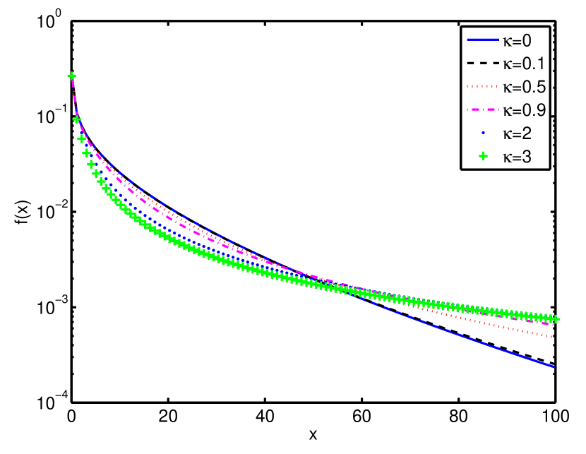
(a) $m=0.7$

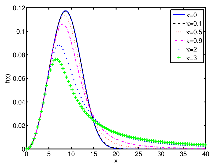
(b) $m=3$

Figure 1: $\kappa$-Weibull pdfs for $x_{s}=10$, different values of $\kappa$, and (a) $m=0.7$ (b) $m=3$.

It is important to note that the $\kappa$-Weibull admits explicit expressions for all the important univariate probability functions. The $\kappa$-Weibull hazard rate function is defined by means of $h_{\kappa}(x)=f_{\kappa}(x)/R_{\kappa}(x)=-d\,\ln R_{\kappa}(x)/dx$, leading to

$$h_{\kappa}(x)=\frac{m}{x_{s}}\frac{\left(x/x_{s}\right)^{m-1}}{\sqrt{1+\kappa^{2}(x/x_{s})^{2m}}}.$$ (15)

The $\kappa$-Weibull quantile function for a given survival probability $r$ is defined by

$$T_{\kappa}(r)=\frac{1}{x_{s}}\left(\ln_{\kappa}{\frac{1}{r}}\right)^{1/m}.$$ (16)

In addition, if we define ${\Phi^{\prime}}_{\kappa}(x)=\ln\ln_{\kappa}(1/R_{\kappa}(x))$ it follows that ${\Phi^{\prime}}_{\kappa}(x)=m\ln\left(\frac{x}{x_{s}}\right)$. Hence, ${\Phi^{\prime}}_{\kappa}(x)$ is independent of $\kappa$ and regains the logarithmic scaling of the double logarithm of the inverse survival function.

III.2 RVE Survival Function

We define the RVE cdf at level $x\in[0,\infty)$ through the equation

$$F_{1}(x)=1+\frac{1}{n}\left(\frac{x}{x_{s}}\right)^{m}-\sqrt{1+\frac{1}{n^{2}}\left(\frac{x}{x_{s}}\right)^{2m}}.$$ (17)

$F_{1}(x)$ is a well defined cdf, because $F_{1}(x=0)=0$, whereas for $x>0$ $F_{1}(x)$ is an increasing function of $x$, and $\lim_{x\rightarrow\infty}F_{1}(x)=1.$ This particular form of $F_{1}(x)$ is motivated by arguments similar to those used in the Weibull case. In Section II, the Weibull survival function $R_{n}(x)$ was derived from (1) assuming that the link survival function is $R^{(i)}_{1}(x)={\rm e}^{-\phi(x)}$ where $\phi(x)=(x/x_{s})^{m}.$ Another approach that does not require the exponential dependence of the RVE survival function is based on the following approximation

$$R_{n}(x)=\left[1-F_{1}(x)\right]^{n}\Rightarrow\ln R_{n}(x)=n\,\ln\left[1-F_{1}(x)\right]\approx-n\,F_{1}(x).$$

The above assumes that $F_{1}(x)\ll 1$ for the link cdfs if $n$ is large. Then, assuming that $F_{1}(x)\propto(x/x_{s})^{m}$ the Weibull form is obtained. The dependence of $F_{1}(x)$ for large $x$ which becomes relevant for finite $n$, however, is not specified. In contrast, (17) generalizes the algebraic dependence so that $F_{1}(x)\sim(x/x_{s})^{m}$ for $x\rightarrow 0$, whereas $F_{1}(x)$ is also well defined for $x\rightarrow\infty$.

From (17) it follows that the respective survival function is

$$R_{1}(x)=\sqrt{1+\frac{1}{n^{2}}\left(\frac{x}{x_{s}}\right)^{2m}}-\frac{1}{n}\left(\frac{x}{x_{s}}\right)^{m}.$$ (18)

Application of the weakest-link scaling relation (2) to (18) leads to the following system survival function

$$R_{n}(x)=\left[\sqrt{1+\frac{1}{n^{2}}\left(\frac{x}{x_{s}}\right)^{2m}}-\frac{1}{n}\left(\frac{x}{x_{s}}\right)^{m}\right]^{n}.$$ (19)

The definition (17) implies that $F_{1}(x)$ and $R_{1}(x)$ depend on the number of RVEs, which destroys the weakest-link scaling relation (3). Based on (18) and using $z=(x/x_{s})^{m}$ it follows that

$$\frac{\partial R_{1}(z)}{\partial n}=\frac{z}{n^{2}}\left(1-\frac{z}{\sqrt{z^{2}+n^{2}}}\right)>0,\;\forall z>0.$$

Hence, the survival probability of single RVEs at a given threshold $z$ increases with $n$.

We propose an ansatz which is consistent with the dependence of $R_{1}(x)$ as given by (18). Assume that the system comprises a number of units (e.g., faults) with inter-dependent RVE survival probabilities, as expected in the presence of correlations. Following a renormalization group (RG) procedure, the interacting units are replaced by non-interacting “effective RVEs”. The RG procedure recovers the product form (2) for the survival probability of independent RVEs, while renormalizing the scale parameter $x_{0}$ by the number of effective RVEs. We can think of $\kappa=1/n$ as a measure of the range of interactions versus the size of the system; $\kappa=0$ yields the classical Weibull pdf for infinite systems, whereas $\kappa\uparrow$ implies that the range of correlations increases thus reducing the number of independent units; the case $\kappa=1$ means that the system can not be reduced to smaller independent units.

IV Weakest-Link Scaling and Return Intervals

Below we focus explicitly on earthquake return intervals; thus, we replace $x$ with $\tau$. In earthquake analysis the spatial support includes either a single fault or a system of several faults. The notion of an RVE with respect to earthquakes is neither theoretically developed nor experimentally validated. Hence, herein we assume that the study domain involves $n$ independent, identically distributed RVEs, where $n$ is not necessarily an integer .

An earthquake catalog is a table of the marked point process Daley and Vere-Jones (2003) $C=\{{{\bf s}}_{i},t_{i},M_{i}\}_{i=1,\ldots,N}$, where ${{\bf s}}_{i}$ is the location, $t_{i}$ the time, and $M_{i}$ the magnitude of the seismic event. Given a threshold magnitude $M_{c}$, an ERI sequence comprises the intervals $\{\tau_{j}=t_{j+k}-t_{j}:(M_{j},M_{j+k}>M_{c})\wedge(M_{j+1},\ldots,M_{j+k-1}\leq M_{c})\}$, where $j=1,\ldots,N_{c}-1,$ $N_{c}$ is the number of events with magnitude exceeding $M_{c}$ (Fig. 2), and $\wedge$ is the logical conjunction symbol. The random variable $T_{M_{c}}^{(i)}$ $(i=1,\ldots,n)$ denotes the quiescent interval for the i-th RVE during which no events of magnitude $M>M_{c}$ occur. The cdf $F_{1}(\tau;M_{c})={\rm Prob}(T_{M_{c}}^{(i)}\leq\tau)$ represents the probability of RVE “failure”, i.e., that an event with $M>M_{c}$ occurs on the RVE within time interval $\tau$ from the previous event. In the following, we suppress the dependence on $M_{c}$ for brevity.

Figure 2: Schematic illustrating the definition of a return interval $\tau_{j}$ as the time between two consecutive events with magnitudes  $M_{j}$ and $M_{j+k}$ that exceed the threshold $M_{c}$, i.e., the events occurring at times $t_{j}$ and $t_{j+k}$.

IV.1 Survival Probability Function

The survival probability $R_{1}(\tau)=1-F_{1}(\tau)$ is the probability that no event with magnitude $M>M_{c}$ occurs on the RVE during the interval $T_{M_{c}}^{(i)}\leq\tau$. For $\tau\rightarrow 0$, it follows from (18) that $R_{1}(\tau)\sim 1-\tau^{m}/(n\,\tau_{s}^{m})$. For $\tau\gg 1$ and finite $n$, it follows that $R_{1}(\tau){\sim}n\,\tau_{s}^{m}/{2\tau^{m}}$, and thus $R_{n}(\tau)$ shows the power-law dependence $R_{n}(\tau){\sim}(n/2)^{n}(\tau_{s}/\tau)^{mn}$, characteristic of the Pareto distribution. In addition, $\lim_{n\rightarrow\infty}R_{n}(\tau)=\exp\left[-(\tau/\tau_{s})^{m}\right]$, thus recovering the Weibull survival probability at the limit of an infinite system. The above equation shows that the interval scale for large $n$ saturates at $\tau_{s}$, in contrast with the classical $\tau_{s}\propto n^{-1/m}$ Weibull scaling. Based on the Gutenberg-Richter law of seismicity which predicts exponential decay of earthquake events as $M_{c}\uparrow$, it follows that $\tau_{s}\uparrow$ as $M_{c}\uparrow$. In contrast, $m$ is expected to vary more slowly with $M_{c}$ Hristopulos and Mouslopoulou (2013).

IV.2 Median of Return Intervals

The median of the single RVE distribution is defined by $R_{1}(\tau_{\rm med;1})=0.5$, and based on (18) it is given by $\tau_{\rm med;1}=\tau_{s}\,\left(\frac{3n}{4}\right)^{1/m}.$ The median of the $\kappa$-Weibull distribution Clementi et al. (2009) for a system of $n=1/\kappa$ RVEs is given by $\tau_{{\rm med;}n}=(\ln_{\kappa}2)^{1/m}\,\tau_{s}$, whereas the median of the Weibull distribution is $\underset{n\rightarrow\infty}{\lim}\tau_{{\rm med;}n}=(\ln 2)^{1/m}\tau_{s}$. Based on the above, the ratio of the median return interval for a finite system over the median return interval of an infinite system both of which have the same $\tau_{s}$, is given by $\tau_{{\rm med};n}/\tau_{\rm med;\infty}=\left(\ln_{\kappa}2/\ln 2\right)^{1/m}$. The ratio is plotted in Fig. 3. For $n$ fixed the ratio is reduced with increasing $m$, whereas for $m>1$ the median return interval varies only slightly with $m$. Keeping $m$ fixed, the median return interval ratio declines with $n$ toward 1. This means that smaller systems have higher median return interval than the infinite system —assuming that the characteristic interval does not change with size. This result is related to the heavier (i.e., power-law) upper tail of the finite-size system.

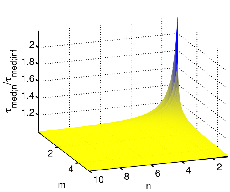
Figure 3: Median ratio $\tau_{{\rm med};n}/\tau_{\rm med;\infty}$ for the $\kappa$-Weibull distribution versus the Weibull modulus $m$ and the system size $n$.

IV.3 Hazard Rate Function

A significant question for seismic risk assessment is whether the probability of an earthquake of given magnitude grows or declines as the waiting time increases Sornette and Knopoff (1997); Corral (2005). An answer to this question involves the hazard rate function of the return intervals. The latter is the conditional probability that an earthquake will occur at time $\tau^{\ast}$ within the infinitesimal time window $\tau<\tau^{\ast}\leq\tau+d\tau$, given that there are no earthquakes in the interval $[0,\tau].$ Hence Sornette and Knopoff (1997),

$$h_{\tau}(\tau)=\frac{{\rm Prob}[\tau<\tau^{\ast}\leq\tau+d\tau|\tau^{\ast}>\tau]}{d\tau}=\frac{f_{\tau}(\tau)}{R(\tau)}.$$

If earthquakes were random (memoryless) processes, distributed in time according to the Poisson law, the ERI would follow the exponential distribution leading to a constant $h_{\tau}(\tau)$. If the ERI follows the Weibull distribution with cdf (4), the hazard rate is given by

$$h_{\tau}(\tau)=\left(\frac{m}{\tau_{s}}\right)\,\left(\frac{\tau}{\tau_{s}}\right)^{m-1}.$$ (20)

According to (20), the hazard rate for $m>1$ increases as $\tau\rightarrow\infty.$ This is believed to apply to characteristic earthquakes that occur on faults located near plate boundaries. In contrast, the Weibull distribution with $m<1$ as well as the lognormal and the power-law distributions exhibit the opposite trend Sornette and Knopoff (1997).

Since Bak proposed a connection between earthquakes and self-organized criticality Bak et al. (2002), universal or locally modified power-law expressions and the gamma probability density function —which is a power law with an exponential cutoff for large times— have been proposed as models of the ERI pdf Corral (2006); Saichev and Sornette (2006); Touati et al. (2009); Baró et al. (2013). The behavior of the gamma distribution depends on the value of the power-law exponent in the same way as the Weibull model. An analysis of two earthquake catalogues based on the gamma distribution concludes that the hazard rate decreases with time (corresponding to an exponent between 0 and 1) Corral (2005).

The hazard rate of the $\kappa$-Weibull is given by (15). For finite $n$ and for $\tau\gg\tau_{s}\,n^{1/m}$, $h_{\tau}(\tau)\sim 1/\tau$. If we take the limit $n\rightarrow\infty$ before $\tau\rightarrow\infty$, the Weibull hazard rate (20) is obtained. For a fixed RVE size, even if $n\gg 1$, the Weibull scaling holds for $\tau<\tau_{s}\,n^{1/m}$ whereas for $\tau\gg\tau_{s}\,n^{1/m}$ the $\tau^{-1}$ scaling dominates. This behavior of $h(\tau)$ is demonstrated in Fig. 4:

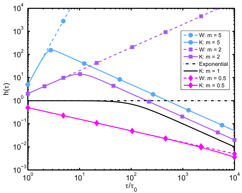
Figure 4: Log-log plot of hazard rates $h(\tau)$ versus $\tau$ for different models. (K): $\kappa$-Weibull hazard rate based on (15) for $n=100$ with $m=0.5$ (magenta solid line and diamonds), $m=1$ (black solid line), $m=2$ (purple solid line with squares), and $m=5$ (cyan line with circles). (W): Weibull hazard rate obtained from (20) with $m=0.5$ (magenta dashed line with diamonds), $m=2$ (purple dashed line with squares), $m=5$ (cyan dashed line with circles). (Exponential): Exponential hazard rate obtained from (20) with $m=1$ (black dash-dot line).

For $m<1$ the dependence is not severely affected by size effects; for $m=1$ there is a constant plateau followed by an $1/\tau$ decay, whereas for $m>1$ the initial increase of $h(\tau)$ turns into an $1/\tau$ decay after a turning point which occurs for $\tau_{c}\approx\tau_{s}\,n^{1/m}.$

V Analysis of Earthquake Return Interval Data

The estimation of the ERI distribution from data is complicated by the fact that the $\kappa$-Weibull distribution and the Weibull distribution are close over the range $0\leq\tau\leq\tau_{w}$, where $\tau_{w}$ is a parameter that depends on $n$ and $m$. Differences in the tail of ERI distributions are best visualized in terms of $\Phi_{n}(\tau)$, as shown in the Weibull plots of Figs. 5-6. On these diagrams, the deviation of the $\kappa$-Weibull distribution from the straight line diminishes with increasing $n$. The gamma distribution is also included for comparison purposes. The gamma probability model with pdf $f(\tau)=\tau^{\alpha-1}\exp(-\tau/b)\big{/}b^{\alpha}\Gamma(\alpha)$ is often used in studies of earthquake return intervals, e.g. Corral (2003),Corral (2005). For $m<1$ the Weibull plot of the gamma probability distribution is a convex function, whereas for $m>1$ it becomes concave. In contrast, the $\kappa$-Weibull distribution is concave for all $m$.

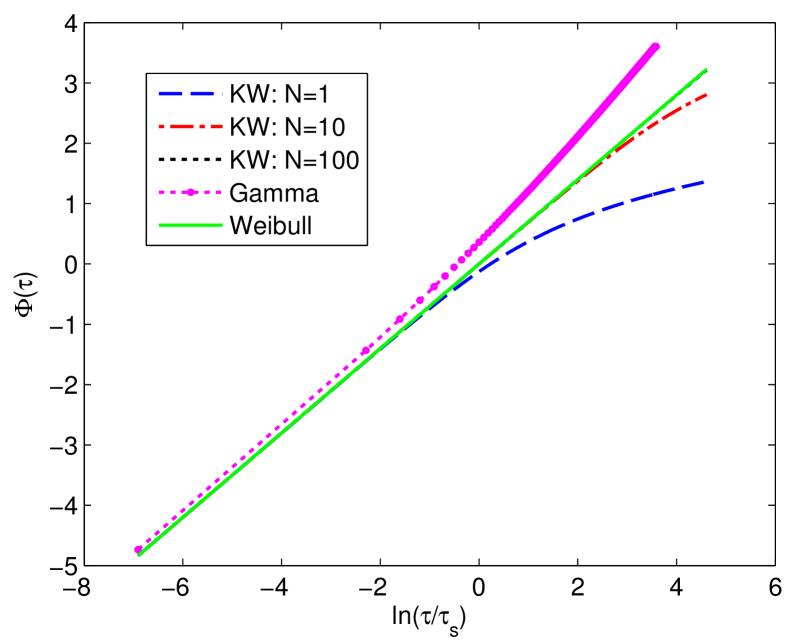
Figure 5: $\Phi_{n}(\tau)$ versus $\ln(\tau/\tau_{s})$ for the Weibull distribution with $m=0.7$ (green solid line), the $\kappa$-Weibull with $m=0.7$ and $n=1$ (blue dashed line), $n=10$ (red dashed and dotted line), $n=100$ (black dotted line), and the gamma distribution with $\alpha=0.7$ (magenta dashed line with small circles).

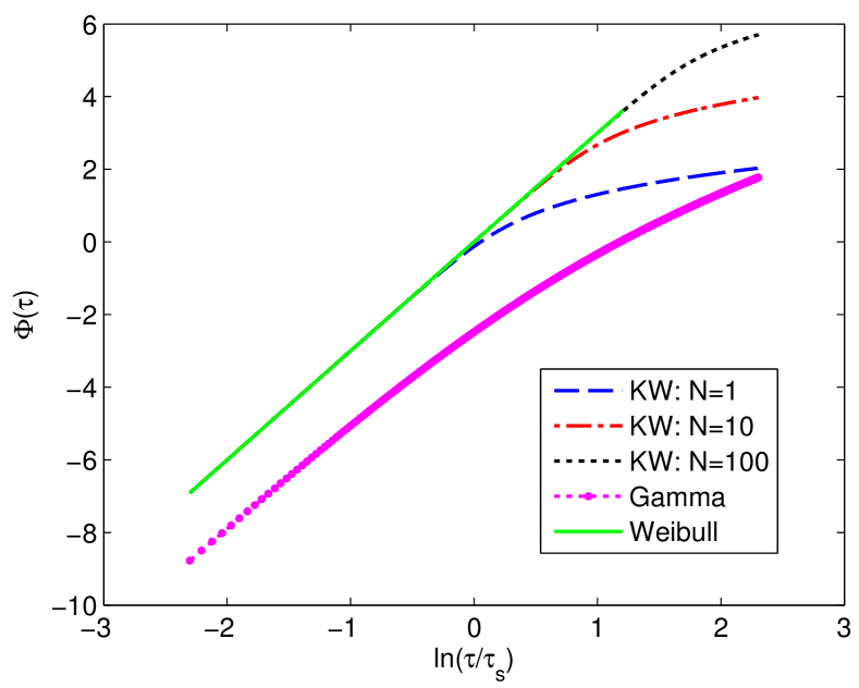
Figure 6: $\Phi_{n}(\tau)$ versus $\ln(\tau/\tau_{s})$ for the Weibull distribution with $m=3$ (green solid line), the $\kappa$-Weibull with $m=3$ and $n=1$ (blue dashed line), $n=10$ (red dashed and dotted line), $n=100$ (black dotted line), and the gamma distribution with $\alpha=3$ (magenta dashed line with small circles).

V.1 Microseismic sequence from Crete

We consider the return intervals for an earthquake sequence from the island of Crete (Greece) which involves over 1 821 micro-earthquake events with magnitudes up to 4.5 (${\rm M_{L}}$) (Richter local magnitude scale) Hristopulos and Mouslopoulou (2013). The sequence was recorded between July 2003 and June 2004 Hristopulos and Mouslopoulou (2013). The return intervals between successive earthquake events range from 1 (sec) to 19.5 (days). The spatial domain covered is approximately between $24.5^{\circ}$ – $27^{\circ}$ (East longitude) and $34^{\circ}$ – $35.5^{\circ}$ (North latitude). The magnitude of completeness for this data set is around 2.2 – 2.3 (${\rm M_{L}}$), which means that all events exceeding this magnitude are registered by the measurement network.

We use the method of maximum likelihood to estimate the parameters of test probability distributions for the return intervals. The optimal $\kappa$-Weibull distribution for events above $M_{c}=2.3$ (${\rm M_{L}}$) is compared with the optimal Weibull distribution in Fig. 7 . Note that the empirical distribution of the return intervals has $m<1$ and a concave tail, in contrast with the gamma density model (cf. Fig. 5). The $\kappa$-Weibull distribution approximates better the upper tail of the return intervals than the Weibull distribution. Both the Weibull distribution and the $\kappa$-Weibull distribution have a lighter lower tail than the data. These trends persist as $M_{c}\uparrow$, but the differences between the distributions progressively decrease. Fig. 8 compares the quantiles of the data distribution with those of the optimal $\kappa$-Weibull model.

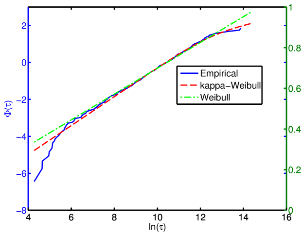
Figure 7: $\Phi(\tau)$ versus $\ln(\tau)$ for earthquake return intervals of the Cretan earthquake sequence (CES). The return intervals refer to 628 events with magnitudes exceeding 2.3 (${\rm M_{L}}$). The magnitude of completeness is $\approx 2.2$ (${\rm M_{L}}$). The maximum likelihood estimates of the $\kappa$-Weibull parameters are $\hat{\tau}_{0}\approx 3.19\times 10^{4}$ (sec), $\hat{m}\approx 0.78$, $\hat{\kappa}\approx 0.33$. The estimate of $\Phi(\tau)$ using the empirical (data-based) cdf is shown with the solid blue line. The optimal $\kappa$-Weibull fit is shown with the red dashed line, whereas the optimal Weibull fit is shown with the green dashed and dotted line. The left vertical axis measures $\Phi(\tau)$, whereas the right vertical axis marks the corresponding cdf values.

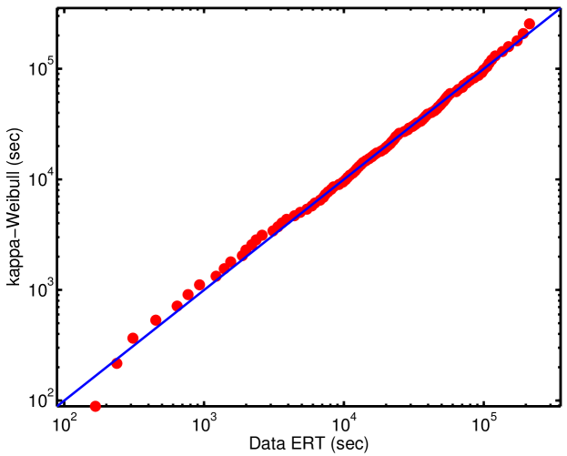
Figure 8: Sample quantiles versus the corresponding quantiles of the optimal $\kappa$-Weibull distribution for the Cretan earthquake sequence return intervals (CES ERI) —$\Phi(\tau)$ of the data shown in Fig. 7. The $\kappa$-Weibull quantiles are obtained from (16) using the maximum likelihood estimates of the $\kappa$-Weibull parameters (see caption of Fig. 7).

We investigate different hypotheses for the ERI distribution using the Kolmogorov-Smirnov test following the methodology described in Clauset et al. (2009). The Kolmogorov-Smirnov distance between the empirical (data) distribution, ${F}_{\rm emp}(\tau)$ and the estimated (model) distribution, $\hat{F}(\tau)$, is given by $D=\sup_{\tau\in\mathbb{R}}|{F}_{\rm emp}(\tau)-\hat{F}(\tau)|$, where $\sup_{A}f(\tau)$ denotes the supremum of $f(\tau)$ for $\tau\in A$. The parameters of $\hat{F}(\tau)$ are also estimated using the method of maximum likelihood as described above. The null hypothesis is that $\hat{F}(\tau)$ represents the probability distribution of the data. We apply the test to the Poisson, normal (Gaussian), lognormal, Weibull, $\kappa$-Weibull, gamma, and generalized gamma distributions. The generalized gamma distribution Stacy (1962), with pdf given by $f(x)=(d/x_{s})^{m}\,x^{d-1}\,{\rm e}^{-(x/x_{s})^{m}}\big{/}\Gamma(d/m)$, incorporates both the gamma distribution (for $m=1$) and the Weibull distribution (for $m=d$).

The Kolmogorov-Smirnov test for a probability model with estimated parameters should be applied using Monte Carlo simulation to generate synthetic data from the estimated probability model. We generate random numbers from the Poisson, normal, lognormal, Weibull, and gamma distributions with the respective MATLAB random number generators. For the $\kappa$-Weibull ($\kappa>0$) and for the generalized gamma distribution we implemented the inverse transform sampling method (see Appendix A). For each realization of return intervals, we estimate the parameters of the optimal distribution model, $\hat{F}^{(j)}(\tau),j=1,\ldots,N_{\rm sim}$. The Kolmogorov-Smirnov distance between the empirical distribution of the specific realization, ${F}^{(j)}_{\rm emp}(\tau)$, and the estimated model distributions for the $j^{\rm th}$ realization are given by $D^{(j)}=\sup_{\tau\in\mathbb{R}}|{F}^{(j)}_{\rm emp}(\tau)-\hat{F}^{(j)}(\tau)|,\;j=1,\ldots,N_{\rm sim}$. The $p$-value of the Kolmogorov-Smirnov distance is defined as $p=\frac{1}{N_{\rm sim}}\sum_{i=j}^{N_{\rm sim}}\mathbbm{1}_{D^{(j)}>D}(D^{(j)})$ —where $\mathbbm{1}_{A}(\tau)=1$, if $\tau\in A$ and $\mathbbm{1}_{A}(\tau)=0$, if $\tau\notin A$, is the indicator function of the set $A$. The $p$-value is the probability the Kolmogorov-Smirnov distance will exceed $D$ purely by chance if the null hypothesis is true. If $p>p_{\rm crit}$, the null hypothesis is accepted, otherwise it is rejected.

If we focus on the return intervals between earthquakes with magnitudes exceeding $2.3$, the Kolmogorov-Smirnov test (based on $1\,000$ simulations) rejects the normal, gamma, and lognormal and Poisson distributions at the $5\%$ significance level. In contrast, the Weibull and $\kappa$-Weibull distributions are accepted with $p\approx 0.09$ and $p\approx 0.75$, respectively, whereas the generalized gamma at $p\approx 0.10$. For $3.5\geq M_{c}\geq 2.3$ (${\rm M_{L}}$) the calculated $p$-values are shown in Table 1. The following remarks summarize the tabulated results: (i) The $\kappa$-Weibull and the Weibull distributions are accepted for all $M_{c}$ except for 2.7 and 3.5. (ii) The gamma distribution is accepted for $M_{c}\geq 2.5$ whereas the generalized gamma is accepted for all $M_{c}$ except for $M_{c}=2.7$. (iii) The lognormal is marginally accepted for $M_{c}=3.5$. (iv) The Poisson distribution is accepted for $M_{c}=3.7,3.9$ (v) The normal and Poisson models are rejected for all $M_{c}\leq 3.7$. (vi) For $M_{c}\leq 3.3$ the Weibull, the gamma, generalized gamma and the $\kappa$-Weibull models have the highest $p$-values but their relative ranking changes with $M_{c}$. Note that for $M_{c}>3.3$ the sample size is quite small $(45\geq N_{c}\geq 18)$ thus prohibiting the observation of long tails.

Table 1: $p$-values of Kolmogorov-Smirnov test for the fit between different probability models and the Crete Earthquake Sequence. Results are based on $1\,000$ simulations. The sample size (number of return intervals) is shown within parentheses next to the cutoff magnitudes.

	Gamma	Weibull	$\kappa$-Weibull	Gen. Gamma	Normal	Lognormal	Poisson
$M_{L,c}=$2.3 (628)	0.00	0.09	0.75	0.10	0.00	0.00	0.00
$M_{L,c}=$2.5 (414)	0.07	0.40	0.14	0.35	0.00	0.00	0.00
$M_{L,c}=$2.7 (273)	0.38	0.01	0.00	0.04	0.00	0.00	0.00
$M_{L,c}=$2.9 (176)	0.14	0.23	0.20	0.25	0.00	0.00	0.00
$M_{L,c}=$3.1 (103)	0.28	0.27	0.20	0.40	0.00	0.00	0.00
$M_{L,c}=$3.3 (69)	0.28	0.11	0.10	0.19	0.00	0.01	0.00
$M_{L,c}=$3.5 (45)	0.15	0.03	0.03	0.08	0.00	0.05	0.00
$M_{L,c}=$3.7 (28)	0.16	0.10	0.08	0.07	0.00	0.00	0.14
$M_{L,c}=$3.9 (18)	0.20	0.19	0.17	0.09	0.27	0.02	0.25

Since for most $M_{c}$ more than one model hypotheses pass the Kolmogorov-Smirnov test, it is desirable to somehow compare the different probability models. For this purpose we use the Akaike Information Criterion (AIC) Akaike (1974). The AIC is defined by $\mathrm{AIC}=2\,\mathrm{NLL}+2k$, where $\mathrm{NLL}$ is the negative log-likelihood of the data for the given model, and $k$ is the number of model parameters ($k=1$ for the Poisson, $k=2$ for the normal, lognormal, Weibull, and gamma, whereas $k=3$ for the $\kappa$-Weibull and the generalized gamma). The term $2k$ in AIC penalizes models with more parameters. In general, a model with lower AIC is preferable to one with higher AIC. We present AIC results for the Crete Earthquake Sequence in Table 2. The tabulated values correspond to $\mathrm{AIC}/N_{c}$. The following conclusions can be reached from this Table: (i) The gamma, generalized Weibull, and $\kappa$-Weibull distributions have similar AIC values which are lower than the normal, lognormal, and Poisson models. (ii) The AIC values of the four top ranking distributions are quite close to each other. (iii) The $\kappa$-Weibull has the lowest AIC for the larger samples (i.e., those with $M_{c}=2.3,2.5$). The observation (i) also explains the somewhat unexpected outcome of Table 1, namely, that the $p$-values of the generalized gamma and the $\kappa$-Weibull are not —for all magnitude cutoffs— equal or higher than the $p$-values of the respective subordinated distributions, i.e., the gamma and the Weibull respectively: The estimates of the probability model parameters are based on the minimization of the negative log-likelihood, which provides a different measure of the fit between the data and the model distribution than the Kolmogorov-Smirnov distance. We checked that the incongruence remains even if the likelihood optimization algorithm for the generalized gamma and the $\kappa$-Weibull is initialized by the respective optimal parameters of the gamma and Weibull distributions for the same data set.

Table 2: Akaike Information Criterion (AIC) values per sample point for different probability models. The model parameters used maximize the likelihood of the Crete Earthquake Sequence given the respective model. The sample size (number of return intervals) is shown within parentheses next to the cutoff magnitudes.

	Gamma	Weibull	$\kappa$-Weibull	Gen. Gamma	Normal	Lognormal	Poisson
$M_{L,c}=$2.3 (628)	23.23	23.16	23.12	23.15	25.95	23.21	23.46
$M_{L,c}=$2.5 (414)	24.05	24.02	24.00	24.02	26.40	24.12	24.29
$M_{L,c}=$2.7 (273)	24.91	24.90	24.90	24.90	26.89	25.07	25.12
$M_{L,c}=$2.9 (176)	25.79	25.78	25.79	25.79	27.59	25.91	26.00
$M_{L,c}=$3.1 (103)	26.81	26.80	26.82	26.82	28.56	26.92	27.08
$M_{L,c}=$3.3 (69)	27.58	27.59	27.62	27.62	29.23	27.76	27.86
$M_{L,c}=$3.5 (45)	28.17	28.20	28.24	28.23	30.22	28.38	28.57
$M_{L,c}=$3.7 (28)	29.30	29.36	29.43	29.41	30.67	29.79	29.46
$M_{L,c}=$3.9 (18)	30.37	30.43	30.54	30.50	31.08	30.92	30.38

V.2 Southern California Data

We also analyze an earthquake sequence which contains 2 446 events in Southern California ($114^{\circ}$ – $122^{\circ}$ West longitude and $32^{\circ}$ – $37^{\circ}$ North latitude) down to depths of $\leq 20$ (km) with magnitudes from 1 (except for 3 events at 0.5) up to 6.5 (${\rm M_{L}}$); 2 444 of these events have magnitudes less than 5.0 (${\rm M_{L}}$), whereas the two main shocks have 6.0 (${\rm M_{L}}$) and 6.5 (${\rm M_{L}}$). The events occurred during the period from January 1, 2000 until March 27, 2012 .

The $p$-values of the Kolmogorov-Smirnov test are listed in Table 3. The Weibull and $\kappa$-Weibull distributions have practically the same $p$-values. The gamma and generalized gamma models, however, show overall better agreement with the observed return intervals than the Weibull or the $\kappa$-Weibull. Most of the $p$-values obtained for this data set are considerably lower than their counterparts for the Cretan data set. To ensure that this difference is not caused by an insufficient number of Monte Carlo simulations, we repeated the numerical experiment with $5\,000$ Monte Carlo simulations, which confirmed the results of Table 3 with minor changes in the $p$-values. On the other hand, as shown in Table 4, the gamma, generalized gamma, Weibull and $\kappa$-Weibull distributions have similar AIC values. The low $p$-values are an indication that none of the models tested match the data very well in terms of the Kolomogorov-Smirnov distance. The gamma, generalized gamma, Weibull and $\kappa$-Weibull, however, are not rejected at the $1\%$ level for most thresholds. It should be noted that recent arguments based on Bayesian analysis of hypothesis testing suggest that the significance level $0.05$ used to reject the null hypothesis is overly conservative and should be shifter to $0.005$ Johnson (2013).

Table 3: $p$-values of Kolmogorov-Smirnov test for the fit between different probability models and the Southern California sequence. Results are based on $5\,000$ simulations. The sample size (number of return intervals) is shown within parentheses next to the cutoff magnitudes.

	Gamma	Weibull	$\kappa$-Weibull	Gen. Gamma	Normal	Lognormal	Poisson
$M_{L,c}=$2.3 (1341)	0.0296	0.0000	0.0000	0.0000	0.0000	0.0000	0.0000
$M_{L,c}=$2.5 (964)	0.0368	0.0000	0.0000	0.0000	0.0000	0.0000	0.0000
$M_{L,c}=$2.7 (687)	0.0348	0.0000	0.0000	0.0000	0.0000	0.0000	0.0000
$M_{L,c}=$2.9 (457)	0.0908	0.0002	0.0004	0.0000	0.0000	0.0000	0.0000
$M_{L,c}=$3.1 (309)	0.5036	0.0638	0.0556	0.0440	0.0000	0.0000	0.0000
$M_{L,c}=$3.3 (206)	0.0254	0.0158	0.0150	0.0270	0.0000	0.0000	0.0000
$M_{L,c}=$3.5 (121)	0.1836	0.0110	0.0086	0.0152	0.0000	0.0000	0.0000
$M_{L,c}=$3.7 (77)	0.0798	0.0304	0.0258	0.0412	0.0000	0.0002	0.0000
$M_{L,c}=$3.9 (44)	0.0150	0.0450	0.0378	0.0580	0.0000	0.0964	0.0000

Table 4: Akaike Information Criterion (AIC) values per sample point for the best-fit models of the Southern California sequence. The model parameters used maximize the likelihood of the Southern California sequence given the respective model. The sample size (number of return intervals) is shown within parentheses next to the cutoff magnitudes.

	Gamma	Weibull	$\kappa$-Weibull	Gen. Gamma	Normal	Lognormal	Poisson
$M_{L,c}=$2.3 (1341)	26.45	26.45	26.45	26.44	29.19	26.68	27.14
$M_{L,c}=$2.5 (964)	26.98	27.01	27.01	27.01	29.73	27.26	27.79
$M_{L,c}=$2.7 (687)	27.55	27.59	27.59	27.60	30.33	27.85	28.47
$M_{L,c}=$2.9 (457)	28.36	28.41	28.42	28.40	30.92	28.65	29.29
$M_{L,c}=$3.1 (309)	28.99	29.02	29.03	29.02	31.82	29.22	30.06
$M_{L,c}=$3.3 (206)	29.28	29.30	29.31	29.31	32.69	29.43	30.88
$M_{L,c}=$3.5 (121)	30.03	30.07	30.08	30.08	33.84	30.22	31.84
$M_{L,c}=$3.7 (77)	30.64	30.72	30.81	30.72	34.65	30.89	32.74
$M_{L,c}=$3.9 (44)	30.70	30.67	30.72	30.72	35.68	30.67	33.46

VI Fiber Bundle Models

Fiber Bundle Models (FBM) are simple statistical models that were introduced to study the fracture of fibrous materials Daniels (1945). To date they are used in many research fields, including fracture of composite materials Phoenix and Tierney (1983), landslides Cohen et al. (2009), glacier avalanches Reiweger et al. (2009) and earthquake dynamics Chakrabarti and Benguigui (1997); Alava et al. (2006); Abaimov et al. (2008). In spite of their conceptual simplicity, FBMs exhibit surprisingly rich behavior.

An FBM consists of an arrangement of parallel fibers subject to an external load $F$ (Fig. 9). The fibers have random strength thresholds that represent the heterogeneity of the medium. Due to the applied loading, each fiber is deformed and subject to stress. If the stress applied to a specific fibre exceeds its failure threshold, the fiber ruptures and the excess load is redistributed either globally or locally between the remaining fibers. The ensuing redistribution of the load to the surviving fibers may trigger an avalanche of breaks. Each fibre break releases the elastic energy accumulated in the fibre.

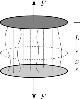
Figure 9: Schematic of a fiber bundle of initial length $L$ elongated by $x$ due to the loading force $F$. Broken fibers do not contribute to the strength of the bundle.

VI.1 FBM Return Interval Statistics

We assume that the strain $\epsilon$ of the fiber bundle increases linearly with time $t$, i.e., $\epsilon\propto t$. Without loss of generality we set the elastic modulus, the initial length $L$ and the strain rate equal to unity, and we use the elongation $x$ instead of $\epsilon$ to measure the loading. The individual fibers have random failure thresholds $x_{\rm c}$ with pdf $f_{\rm x_{\rm c}}(x)$. Failed fibers are removed, and the stress is then redistributed between the surviving fibers using the equal load sharing rule. The energy of each avalanche is equal to the sum of the Hookean energies of the broken fibers Pradhan and Hemmer (2008). Only events that exceed an energy threshold $E_{\rm c}$ are counted. The return intervals are measured as the time difference between two events with energy $E\geq E_{\rm c}$. Avalanches are considered to occur instantaneously. Fig. 10 illustrates the evolution of the avalanche events in time. The plots are obtained by loading a single bundle of $10^{7}$ fibers the strength of which follows the Weibull pdf with $m=5,x_{s}=1$. The avalanche sequences correspond to energy thresholds given by $\log_{10}E_{c}=1,2$, where $\log_{10}$ is the logarithm with base 10.

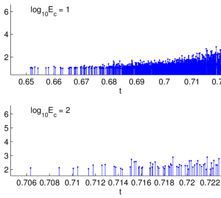
Figure 10: Evolution of avalanche events in time for a bundle of $10^{7}$ fibers with Weibull-distributed strength thresholds ($m=5,x_{s}=1$). The most energetic avalanche $(\log_{10}E_{f}\approx 7.31)$ is generated when the bundle fails (during the last event of the breaking sequence) at time $t_{f}\approx 0.725$.

Figure 11 compares the quantiles of the return interval distribution obtained from a single bundle with those of the optimal $\kappa$-Weibull distribution for different energy thresholds. The optimal $\kappa$-Weibull parameters for each threshold are shown in Table 5. The estimated $\kappa$ values based on maximum likelihood are $\hat{\kappa}\approx 2$. This result suggests that $\kappa>1$ values indicate a highly correlated system that can not be decomposed into RVEs. As stated in Subsection III.1, the $\kappa$-Weibull pdf exhibits a power-law upper tail with exponent $\alpha=1+m/\kappa$. For the FBM investigated above, the exponent of the return interval pdf is $\hat{\alpha}\approx[2.13,2.20]$.

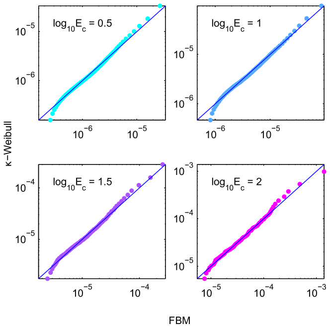
Figure 11: Quantile-quantile plots of FBM return intervals (dimensionless) versus the best-fit $\kappa$-Weibull distribution. Data are based on a bundle of $5\times 10^{7}$ fibers with strength thresholds drawn from the Weibull distribution with $m=5$, $x_{s}=1$, unit elastic constant, and unit strain rate.

Table 5: Maximum Likelihood estimates of $\kappa$-Weibull distribution parameters for the return intervals of Figure 11.

$\log_{10}E_{c}$	$N$	$\hat{\tau}_{s}$	$\hat{m}$	$\hat{\kappa}$
0.5	44094	$1.2\times 10^{-6}$	2.4	2.1
1	8449	$3.7\times 10^{-6}$	2.4	2.0
1.5	1686	$1.0\times 10^{-5}$	2.6	2.2
2	311	$3.1\times 10^{-5}$	2.6	2.3

VII Discussion and Conclusions

We investigated the statistics of return intervals in systems that obey weakest-link scaling. We propose that the $\kappa$-Weibull distribution is suitable for finite-size systems (where the size is measured in terms of RVE size) and that the parameter $\kappa$ is determined by the size of the system. A characteristic property of the $\kappa$-Weibull distribution is the transition from Weibull to power-law scaling in the upper tail of the pdf. This leads to an upper tail which decays slower than the tail of the respective Weibull distribution —a feature useful for describing the statistics of earthquake return intervals. The transition point depends on the system size and the Weibull modulus.

Recent studies have identified a slope change in logarithmic plots of the ERI pdf, attributed to spatial (for earthquakes) or temporal (for lab fracturing experiments) non-stationarity of the background productivity rate Baró et al. (2013). We demonstrated that finite-size effects have a similar impact on the ERI pdf. Hence, finite size can explain deviations of earthquake return intervals from Weibull scaling without invoking non-stationarity (spatial or temporal) in the background earthquake productivity rate.

In addition, we show that a distinct feature of the $\kappa$-Weibull distribution is the dependence of its hazard rate function: for $m>1$ it increases with increasing time interval up to a certain threshold, followed by a $\propto 1/\tau$ drop. This is in contrast with the Weibull hazard rate for $m>1$ which increases indefinitely. Therefore, the $\kappa$-Weibull distribution allows for temporal clustering of earthquakes independently of the value of the Weibull modulus.

The application of the $\kappa$-Weibull distribution to ERI assumes the following:

• Statistical stationarity, i.e., uniform ERI distribution parameters over the spatial and temporal observation window.

• Renormalizability of the interacting fault system into an ensemble comprising a finite number of independent effective RVEs with identical interval scale.

• Specific but simple functional form for the RVE survival probability given by (18).

We believe that the $\kappa$-Weibull distribution is also potentially useful for modeling the fracture strength of heterogeneous quasibrittle structures. The latter involve a finite number of RVEs and their fracture strength obeys weakest-link scaling Bazant and Pang (2006); Bazant et al. (2009). The connection between ERI power-law scaling and fracture mechanics pursued herein and in Hristopulos and Mouslopoulou (2013) also requires further research. Finally, we have used statistical methods (Kolmogorov-Smirnov test, Akaike Information Criterion) to compare different hypotheses for ERI distributions. For example, using the Kolmogorov-Smirnov test we showed that for one sequence of earthquakes the $\kappa$-Weibull, Weibull, gamma, and generalized gamma probability models are acceptable at the $5\%$ level.

Appendix A Inverse Transform Sampling Method

We generate random numbers from the $\kappa$-Weibull and the generalized gamma distributions using the inverse transform sampling method. We first illustrate the algorithm for the $\kappa$-Weibull random numbers.

1. We generate uniform random numbers $u_{\tau}\overset{d}{=}U(0,1)$.

2. We employ the conservation of probability under the variable transformation $\tau\overset{g(\tau)}{\rightarrow}u_{\tau}$, i.e.,

   $$F_{n}(\tau)=F_{U}(u_{\tau})=u_{\tau}\Rightarrow\tau=F^{-1}_{n}(u_{\tau}),$$ (A-21)

   where $F_{n}(\tau)=\left(\sqrt{1+a^{2}\tau^{2m}/n^{2}}-a\tau^{m}/n\right)^{n}$ and $a=\tau_{s}^{-m}$.

3. The above in light of (A-21) leads to

   $$\tau=F^{-1}_{n}(u_{\tau})=\left(\frac{n}{2}\right)^{1/m}\,\tau_{s}\,\left(u^{-1/n}_{\tau}-u^{1/n}_{\tau}\right)^{1/m}=\tau_{s}\,\left[-\ln_{\kappa}(u_{\tau})\right]^{1/m},\quad\kappa=n^{-1}.$$ (A-22)

In the case of the generalized gamma, the cumulative probability distribution is given by

$$F_{n}(\tau)=\gamma\left(\frac{k}{m},(\tau/\tau_{s})^{m}\right),$$ (A-23)

where $\gamma(\alpha,x)$ is the incomplete gamma function defined by

$$\gamma(\alpha,x)=\frac{1}{\Gamma(\alpha)}\int_{0}^{x}dy\,\frac{y^{\alpha-1}}{\tau_{s}^{\alpha}}\,{\rm e}^{-y/\tau_{s}}.$$

The random numbers $\tau$ are then given by inverting $\gamma(\alpha,x(\tau))=u_{\tau}$, that is by

$$\tau=\tau_{s}\,\left[\gamma^{-1}_{n}(\alpha;u_{\tau})\right]^{1/m}.$$

References

- Note (1) The term reverse Weibull refers to the distribution for maxima; this is known as the Weibull distribution in physical sciences and engineering.
- Note (2) Counterpart distributions with reversed supports are obtained for maxima.
- Gumbel (1935) E. J. Gumbel, Ann. Inst. Henri Poincaré 5, 115 (1935).
- Weibull (1951) W. Weibull, J. Appl. Mech. 18, 293 (1951).
- Sornette (2004) D. Sornette, Critical Phenomena in Natural Sciences (Springer, Berlin, 2004).
- Eliazar and Klafter (2006) I. Eliazar and J. Klafter, Physica A 367, 106 (2006).
- Franzke (2012) C. Franzke, Phys. Rev. E 85, 031134 (2012).
- Nicolis and Nicolis (2012) C. Nicolis and G. Nicolis, Phys. Rev. E 85, 056217 (2012).
- de S. Cavalcante et al. (2013) H. L. D. de S. Cavalcante, M. Oriá, D. Sornette, E. Ott, and D. J. Gauthier, Phys. Rev. Lett. 111, 198701 (2013).
- Tallakstad et al. (2013) K. T. Tallakstad, R. Toussaint, S. Santucci, and K. J. Måløy, Phys. Rev. Lett. 110, 145501 (2013).
- Hristopulos and Mouslopoulou (2013) D. T. Hristopulos and V. Mouslopoulou, Physica A 392, 485 (2013).
- Note (3) The terms interevent times, waiting times and recurrence intervals are also used. A subtle distinction can be made between recurrence intervals, which refer to events that take place on the same fault, and interocurrence intervals which encompass all faults in a specified region Abaimov et al. (2008). The statistical properties of recurrence intervals are more difficult to estimate, because less information is available for individual faults. The distinction is, nevertheless, conceptually important, since recurrence intervals characterize the one-body, i.e., the single-fault, problem, while interoccurrence intervals are associated with the activity of the many-body system Sornette (1999). Herein we use the term return intervals without further distinction.
- Sornette (1999) D. Sornette, Phys. Rep. 313, 237 (1999).
- Zhuang et al. (2012) J. Zhuang, D. Harte, M. J. Werner, S. Hainzl, and S. Zhou, Community Online Resource for Statistical Seismicity Analysis (2012), 10.5078/corssa-79905851, available at http://www.corssa.org.
- Bak et al. (2002) P. Bak, K. Christensen, L. Danon, and T. Scanlon, Phys. Rev. Lett. 88, 178501 (2002).
- Corral (2003) A. Corral, Phys. Rev. E 68, 035102 (2003).
- Saichev and Sornette (2007) A. Saichev and D. Sornette, J. Geophys. Res. 112, B04313/1 (2007).
- Klein et al. (1997) W. Klein, J. B. Rundle, and C. D. Ferguson, Phys. Rev. Lett. 78, 3793 (1997).
- Serino et al. (2011) C. A. Serino, K. F. Tiampo, and W. Klein, Phys. Rev. Lett. 106, 108501 (2011).
- Corral (2004) A. Corral, Phys. Rev. Lett. 92, 108501 (2004).
- Corral (2006) A. Corral, Phys. Rev. Lett. 97, 178501 (2006).
- Corral and Christensen (2006) A. Corral and K. Christensen, Phys. Rev. Lett. 96, 109801 (2006).
- Saichev and Sornette (2006) A. Saichev and D. Sornette, Phys. Rev. Lett. 97, 078501 (2006).
- Ogata (1988) Y. Ogata, J. Am. Stat. Assoc. 83, 9 (1988).
- Hagiwara (1974) Y. Hagiwara, Tectonophysics 23, 313 (1974).
- Rikitake (1976) T. Rikitake, Tectonophysics 35, 335 (1976).
- Rikitake (1991) T. Rikitake, Tectonophysics 199, 121 (1991).
- Sieh et al. (1989) K. Sieh, M. Stuiver, and D. Brillinger, J. Geophys. Res. 94, 603 (1989).
- Yakovlev et al. (2006) G. Yakovlev, D. L. Turcotte, J. B. Rundle, and P. B. Rundle, Bull. Seismol. Soc. Am. 96, 1995 (2006).
- Holliday et al. (2006) J. R. Holliday, J. B. Rundle, D. L. Turcotte, W. Klein, K. F. Tiampo, and A. Donnellan, Phys. Rev. Lett. 97, 238501 (2006).
- Abaimov et al. (2007) S. G. Abaimov, D. L. Turcotte, and J. B. Rundle, Geophys. J. Int. 170, 1289 (2007).
- Abaimov et al. (2008) S. G. Abaimov, D. Turcotte, R. Shcherbakov, J. B. Rundle, G. Yakovlev, C. Goltz, and W. I. Newman, Pure Appl. Geophys. 165, 777 (2008).
- Hasumi et al. (2009a) T. Hasumi, T. Akimoto, and Y. Aizawa, Physica A 388, 483 (2009a).
- Hasumi et al. (2009b) T. Hasumi, T. Akimoto, and Y. Aizawa, Physica A 388, 491 (2009b).
- Santhanam and Kantz (2008) M. S. Santhanam and H. Kantz, Phys. Rev. E 78, 051113 (2008).
- Hristopulos and Uesaka (2004) D. T. Hristopulos and T. Uesaka, Phys. Rev. B 70, 064108 (2004).
- Pang et al. (2008) S.-D. Pang, Z. Bazant, and J.-L. Le, Int. J. Fract. 154, 131 (2008).
- Bazant et al. (2009) Z. P. Bazant, J.-L. Le, and M. Z. Bazant, Proc. Natl. Acad. Sci. U.S.A. 1061, 11484 (2009).
- Amaral et al. (2008) P. M. Amaral, L. G. Rosa, and J. C. Fernandes, Rock Mech. Rock Eng. 41, 917–928 (2008).
- Baró et al. (2013) J. Baró, A. Corral, X. Illa, A. Planes, E. K. H. Salje, W. Schranz, D. E. Soto-Parra, and E. Vives, Phys. Rev. Lett. 110, 088702 (2013).
- Main (2013) I. Main, Phys. 6, 20 (2013).
- Curtin (1998) W. A. Curtin, Phys. Rev. Lett. 80, 1445 (1998).
- Alava et al. (2006) M. J. Alava, P. K. V. V. Nukala, and S. Zapperi, Adv. Phys. 55, 349 (2006).
- Alava et al. (2009) M. J. Alava, P. K. V. V. Nukala, and S. Zapperi, J. Phys. D 42, 214012 (2009).
- Chakrabarti and Benguigui (1997) B. K. Chakrabarti and L. G. Benguigui, Statistical Physics of Fracture and Breakdown in Disordered Systems (Clarendon Press, Oxford, UK, 1997).
- Bazant and Pang (2006) Z. P. Bazant and S.-D. Pang, Proc. Natl. Acad. Sci. U.S.A. 103, 9434 (2006).
- Note (4) We assume a fixed RVE size with volume .
- Daniels (1945) H. E. Daniels, Proc. R. Soc. London Ser. A 183, 405 (1945).
- Smith and Phoenix (1981) R. L. Smith and S. L. Phoenix, J. Appl. Mech. 48, 75 (1981).
- Phoenix et al. (1997) S. Phoenix, M. Ibnabdeljalil, and C.-Y. Hui, Int. J. Solids Struct. 34, 545 (1997).
- Eliazar and Metzler (2012) I. Eliazar and R. Metzler, J. Chem. Phys. 137, 234106 (2012).
- Eliazar and Metzler (2013) I. Eliazar and R. Metzler, Phys. Rev. E 87, 022141 (2013).
- Bazant and Pang (2007) Z. P. Bazant and S.-D. Pang, J. Mech. Phys. Solids 55, 91 (2007).
- Eliazar and Klafter (2004) I. Eliazar and J. Klafter, Physica A 334, 1 (2004).
- Kaniadakis (2009) G. Kaniadakis, Eur. Phys. J. B 70, 3 (2009).
- Kaniadakis (2001) G. Kaniadakis, Phys. Lett. A 288, 283 (2001).
- Kaniadakis (2005) G. Kaniadakis, Phys. Rev. E 72, 036108 (2005).
- Kaniadakis (2009) G. Kaniadakis, Eur. Phys. J. A 40, 275 (2009).
- Lapenta et al. (2007) G. Lapenta, S. Markidis, A. Marocchino, and G. Kaniadakis, Astrophys. J. 666, 949 (2007).
- Kaniadakis (2013) G. Kaniadakis, Entropy 15, 3983 (2013).
- Clementi et al. (2007) F. Clementi, M. Gallegati, and G. Kaniadakis, Eur. Phys. J. B 57, 187 (2007).
- Clementi et al. (2008) F. Clementi, T. Di Matteo, M. Gallegati, and G. Kaniadakis, Physica A 387, 3201 (2008).
- Clementi et al. (2009) F. Clementi, M. Gallegati, and G. Kaniadakis, J. Stat. Mech.: Theory Exp. P02037 (2009).
- Note (5) The number of RVEs may also depend on the earthquake cutoff magnitude.
- Daley and Vere-Jones (2003) D. J. Daley and D. Vere-Jones, An Introduction to the Theory of Point Processes. Vol. I, 2nd ed. (Springer-Verlag, New York, 2003) pp. xxii+469 .
- Sornette and Knopoff (1997) D. Sornette and L. Knopoff, Bull. Seismol. Soc. Am. 87, 789– (1997).
- Corral (2005) A. Corral, Phys. Rev. E 71, 017101 (2005).
- Touati et al. (2009) S. Touati, M. Naylor, and I. G. Main, Phys. Rev. Lett. 102, 168501 (2009).
- Note (6) We use the MATLAB fmincon constrained minimization function with a trust region reflective algorithm and explicit gradient information to minimize the negative log-likelihood. The method is applied iteratively (i.e., fmincon is called with the last estimate as initial guess) for fifty times. The optimization parameters used are: Maximum number of objective function evaluation , maximum number of iterations , objective function error tolerance . Tests with the data sequences showed that this number of iterations is sufficient for the parameter estimates to converge. The accuracy and precision of the estimates were also tested using synthetic sequences of -Weibull random numbers generated by means of the inversion method.
- Clauset et al. (2009) A. Clauset, C. Shalizi, and M. Newman, SIAM Rev. 51, 661 (2009).
- Stacy (1962) E. W. Stacy, Ann. Math. Stat. 33, 1187 (1962).
- Akaike (1974) H. Akaike, IEEE Trans. Automat. Contr. 19, 716 (1974).
- Note (7) The facilities of the Southern Californian earthquake Data Center (SCEDC), and the Southern California Seismic Network (SCSN), were used for access to waveforms, parametric data, and metadata required in this study. The SCEDC and SCSN are funded through U.S. Geological Survey Grant G10AP00091, and the Southern Californian earthquake Center, which is funded by NSF Cooperative Agreement EAR-0529922 and USGS Cooperative Agreement 07HQAG0008.
- Johnson (2013) V. E. Johnson, Proc. Nat. Acad. Sci. 110, 19313 (2013).
- Phoenix and Tierney (1983) S. L. Phoenix and L.-J. Tierney, Eng. Fract. Mech. 18, 193 (1983).
- Cohen et al. (2009) D. Cohen, P. Lehmann, and D. Or, Water Resour. Res. 45, W10436 (2009).
- Reiweger et al. (2009) I. Reiweger, J. Schweizer, J. Dual, and H. J. Herrmann, J. Glaciol. 55, 997 (2009).
- Gutenberg and Richter (1956) B. Gutenberg and C. F. Richter, Bull. Seismol. Soc. Am. 46, 105 (1956).
- Gutenberg and Richter (1965) B. Gutenberg and C. F. Richter, Seismicity of the Earth and Associated Phenomena (Hafner New York, 1965).
- Pradhan and Hemmer (2008) S. Pradhan and P. C. Hemmer, Phys. Rev. E 77, 031138 (2008).