Comptonization of photons near the photosphere of relativistic outflows

Abstract

We consider the formation of photon spectrum at the photosphere of ultrarelativistically expanding outflow. We use the Fokker-Planck approximation to the Boltzmann equation, and obtain the generalized Kompaneets equation which takes into account anisotropic distribution of photons developed near the photosphere. This equation is solved numerically for relativistic steady wind and the observed spectrum is found in agreement with previous studies. We also study the photospheric emission for different temperature dependences on radius in such outflows. In particular, we found that for $T\propto r^{-2}$ the Band low energy photon index of the observed spectrum is $\alpha\simeq-1$, as typically observed in Gamma Ray Bursts.

1 Introduction

Gamma Ray Burst (GRB) emission originates from plasma which expands relativistically from initial optically thick phase. It necessarily contains the photospheric component which appears when plasma becomes transparent to radiation initially trapped in it (Goodman, 1986; Paczynski, 1986, 1990; Shemi & Piran, 1990).

The fireshell model, see. e.g. Ruffini et al. (2009) pays special attention to this photospheric component. It is identified as P-GRB (proper GRB). Both its energetics and time separation from the peak of the afterglow are predicted, and comparison with observations allowed identification of this component in many GRBs (970228, 991216, 031203, 050315, 050509B, 060218, 060607A, 060614, 071227, 090618, 090902B, 090423 and others).

The impossibility of explaining observed hard low energy slopes of spectra with traditional synchrotron shock models revived the interest in the photospheric emission from relativistic outflows in the recent literature (Mészáros & Rees, 2000; Mészáros et al., 2002; Daigne & Mochkovitch, 2002; Pe’er et al., 2007; Beloborodov, 2010, 2011; Ryde et al., 2011; Pe’er & Ryde, 2011). Reprocessing of thermal emission assumed to originate from the photosphere by nonthermal distribution of electrons is in the basis of more complicated models with dissipation near the photosphere (Rees & Mészáros, 2005; Giannios, 2006; Toma et al., 2011; Ryde et al., 2011; Vurm et al., 2013; Levinson, 2012). Such models successfully reproduce both high energy and low energy parts of observed spectra in some bursts: e.g. GRB090902B, see Ryde et al. (2011). However, the physics of dissipation is poorly understood. Fine tuning is involved, since such dissipation is required to occur very near the photosphere, see e.g. Vurm et al. (2013).

Several papers claim deviations of theoretically computed spectrum, coming from nondissipative photospheres of relativistic outflows, from the Planck shape at low energies. Beloborodov (2010) found the low energy photon index $\alpha=0.4$ (in contrast with $\alpha=1$ for Planck spectrum) solving the radiative transfer equations by Monte Carlo method in the steady relativistic wind. Pe’er (2008) and Pe’er & Ryde (2011) found both analytically and numerically flattening of the spectrum, considering late time emission from the relativistic wind when it switches off with $\alpha\rightarrow 0$ for late emission. This result is obtained considering the probability density function of the last scattering. Ruffini et al. (2013) found that the increased power at low energies with respect to the Planck spectrum (photon indices are, respectively $\alpha=0.82$ and $0.34$ for accelerating and coasting photon thick instantaneous spectra) is the result of temperature distribution across the Photospheric EQuiTemporal Surface (EQTS) (Bianco et al., 2001; Ruffini et al., 2001).

The formation of photon spectrum at the photosphere of ultrarelativistically expanding outflow can be explained as a combination of several effects. Firstly, there is a contribution from different angles with respect to the line of sight of photons, arriving to the observer at the same time from the EQTS. This effect is purely geometrical. Secondly, photons have different comoving temperatures at each point of EQTS and the observed spectrum is a superposition of that comoving spectra, blueshifted to the observer’s reference frame (a multicolor blackbody) (Pe’er & Ryde, 2011). Thirdly, local spectral distortions arise due to the decoupling of photons from the plasma near the photosphere. In this Letter we are concerned with the latter effect. We use the radiative transfer equation for the steady wind model of Beloborodov (2011) with collision integrals obtained as the Fokker-Planck approximation to exact collision integrals of Compton scattering. This equation reduces to the classic Kompaneets equation for the medium at rest. However, here we consider relativistically expanding outflow, implying that anisotropy of the photon field has to be accounted for in the collision integral. We solve numerically this equation and find the observed spectrum of photospheric emission from relativistic wind.

The paper is organized as follows. In Section 2 we present the radiative transfer equation for coasting relativistic wind. In Section 3 we report our numerical results. Conclusions follow.

2 The radiative transfer equation

We start with the radiative transfer equation in spherically symmetric steady (time independent) medium written in comoving frame, with the only exceptions for radius $r$ and Lorentz factor $\Gamma$ being the quantities measured in the laboratory frame (c.f. Beloborodov (2011)):

$$\frac{\mu+\beta}{1+\beta\mu}\frac{\partial n(r,\epsilon,\mu)}{\partial r}+\frac{1-\mu^{2}}{r}\frac{\partial n}{\partial\mu}-\frac{1-\mu^{2}}{r(1+\beta\mu)}\beta\epsilon\frac{\partial n}{\partial\epsilon}$$

$$=\frac{1}{\Gamma(1+\beta\mu)}\frac{\eta-\chi n}{1+\beta\mu},$$ (1)

where $n$ is photon occupation number, $\mu=\cos\vartheta$ parametrizes the angle between the momentum of the photon and the radius vector, $\eta$ and $\chi$ are emission and absorption coefficients, $\epsilon$ is photon energy.

The collision integral takes into account that photons are scattered by the moving medium (see Fukue et al. (1985); Psaltis & Lamb (1997))  and consequently their distribution is anisotropic in the comoving frame:

$$\eta-\chi n =\frac{3n_{e}\sigma_{\mathrm{T}}\epsilon}{16\pi}\Bigg{\{}\left(1-\frac{2\epsilon}{m_{e}c^{2}}\right)$$ (2)

$$\times\int do^{\prime}\left[\left(1+x^{2}\right)n^{\prime}-n\right]$$

$$+\frac{2\epsilon}{m_{e}c^{2}}\int do^{\prime}\left(x^{3}+x\right)n^{\prime}$$

$$+\frac{2kT_{e}}{m_{e}c^{2}}\int do^{\prime}\left(2x^{3}-3x^{2}-2x+1\right)n^{\prime}$$

$$+\frac{1}{m_{e}c^{2}}\int do^{\prime}\left(1+x^{2}\right)\left(1-x\right)$$

$$\times\left(\frac{kT_{e}}{\epsilon^{2}}\frac{\partial}{\partial\epsilon}\epsilon^{4}\frac{\partial}{\partial\epsilon}+\frac{1}{\epsilon^{2}}\frac{\partial}{\partial\epsilon}\epsilon^{4}+2n\frac{\partial}{\partial\epsilon}\epsilon^{2}\right)n^{\prime}\Bigg{\}},$$

where $T_{e}$ is electron comoving temperature, $n_{e}$ is electron comoving density, $m_{e}$ is electron mass, $\sigma_{\mathrm{T}}$ is Thompson cross section, $c$ is the speed of light, $n=n(\epsilon,\mu)$, $n^{\prime}=n(\epsilon,\mu^{\prime})$, $do^{\prime}=d\mu^{\prime}d\phi^{\prime}$, and $x=\sqrt{1-\mu^{2}}\sqrt{1-\mu^{\prime 2}}\cos(\phi-\phi^{\prime})+\mu\mu^{\prime}$. Here prime denotes angles of particles after scattering.

We integrate Eq. (2) over $d\phi$. Then we introduce the Legendre polynomials

$$n(\epsilon,\mu) =\sum_{l}n_{l}(\epsilon)P_{l}(\mu),$$ (3)

$$P_{0} =1,\quad P_{1}=\mu,\quad P_{2}=\frac{3\mu^{2}-1}{2},\quad P_{3}=\frac{5\mu^{3}-3\mu}{2},$$

and transform to a new variable $\rho\equiv n\epsilon^{2}$. Hence we arrive to the final equation

$$\frac{\partial\rho}{\partial r}+\frac{2\rho}{r}+\frac{1}{r(\beta+\mu)}\frac{\partial}{\partial\mu}\left[(1-\mu^{2})(1+\beta\mu)\rho\right]$$ (4)

$$-\beta\frac{1-\mu^{2}}{r(\beta+\mu)}\frac{\partial(\epsilon\rho)}{\partial\epsilon}=\frac{\epsilon^{2}(\eta-\chi n)}{\Gamma(\beta+\mu)}$$

with

$$\epsilon^{2}(\eta-\chi n)=n_{e}\sigma_{\mathrm{T}}\epsilon\Bigg{\{}\left(1-\frac{2\epsilon}{m_{e}c^{2}}\right)$$ (5)

$$\times\left[\rho_{0}+\frac{1}{10}\rho_{2}P_{2}-\rho\right]$$

$$+\frac{2\epsilon}{m_{e}c^{2}}\left(\frac{2}{5}\rho_{1}P_{1}+\frac{3}{70}\rho_{3}P_{3}\right)$$

$$-\frac{2kT_{e}}{m_{e}c^{2}}\left(\frac{1}{5}\rho_{1}P_{1}\frac{3}{10}\rho_{2}P_{2}+-\frac{3}{35}\rho_{3}P_{3}\right)$$

$$+\frac{1}{m_{e}c^{2}}\left[\frac{\partial}{\partial\epsilon}\left(kT_{e}\epsilon^{2}\frac{\partial}{\partial\epsilon}+\epsilon(\epsilon-kT_{e})\right)+2\rho\frac{\partial}{\partial\epsilon}\right]\times$$

$$\times\left(\rho_{0}-\frac{2}{5}\rho_{1}P_{1}+\frac{1}{10}\rho_{2}P_{2}-\frac{3}{70}\rho_{3}P_{3}\right)\Bigg{\}}.$$

In isotropic case $\rho=\rho_{0}$ and the integration of equation (4) over angles gives the Kompaneets equation for the variable $\rho_{0}$ as

$$\frac{\partial\rho}{\partial r}+\frac{2\rho}{r}=\frac{\epsilon^{2}n_{e}\sigma_{\mathrm{T}}}{\Gamma m_{e}c^{2}}\left(1-\frac{2\epsilon}{m_{e}c^{2}}\right)$$ (6)

$$\times\left[\frac{\partial}{\partial\epsilon}\left(kT_{e}\epsilon^{2}\frac{\partial}{\partial\epsilon}+\epsilon(\epsilon-kT_{e})\right)+2\rho\frac{\partial}{\partial\epsilon}\right]\rho.$$

As expected, the photon number conservation holds, that is $\int d\epsilon r^{2}\rho=\mathrm{const}$. When angle dependence is taken into account photon conservation gives

$$\int d\mu d\epsilon(\beta+\mu)r^{2}\rho=\mathrm{const}.$$ (7)

Equation (4) with collision integral (5) is integrated numerically. We introduced the computational grid for angles and energy and applied lines method for evolutionary equations with coordinate $r$ playing the role of time. Implicit numerical scheme is used. Our scheme for the classical Kompaneets equation is similar to the one used in Nagirner et al. (1997). In numerical calculations one has to assume the temperature and number density of electrons dependence on radius. Following Ruffini et al. (2013) we adopt the comoving density profile

$$n_{e}=n_{0}B\left(\frac{R_{0}}{R}\right)^{2},$$ (8)

where $B=\dot{M}c^{2}/L$ is the baryonic loading parameter, $L$ is luminosity at the base of the wind at radius $R_{0}$ and $\dot{M}$ is mass ejection rate. For the comoving temperature we choose

$$T_{e}=T_{0}B\left(\frac{R_{0}}{BR}\right)^{k},$$ (9)

where $T_{0}=(L/(16\pi\sigma_{SB}R_{0}^{2}))^{1/4}$, $\sigma_{SB}$ is Stefan-Boltzmann constant, $k$ is a constant. This model with $k=2/3$ describes coasting steady relativistic wind.

The electron comoving density decreases with increasing laboratory radius, so does the optical depth. Near the photosphere, where the optical depth reaches unity, the coupling between photons and electrons weakens. We assume that electron comoving temperature on the path of photons propagating outwards is decreasing following eq. (9), even when the outflow becomes optically thin. This effect is parametrized by the coefficient $k\geq 2/3$. Electrons are described by the Maxwellian distribution function in the comoving frame with the temperature given by the relation (9).

Since initially the outflow is highly opaque, photons in the beginning have thermal spectrum and isotropic distribution in the comoving reference frame. Near the photosphere the coupling of photons to the medium is due to Compton scattering on electrons.

Before proceeding with steady wind model, we tested our numerical scheme. Considering a uniform optically thick medium with stimulated emission taken into account and neglected, respectively, convergence to Planck and Wien distributions of photons has been verified.

3 Results

The anisotropy of photon distribution near the photosphere in comoving reference frame found by Beloborodov (2011) is an interesting effect which we have also found in our approach. This result is illustrated in Fig. 1.

This effect can be explained from the geometric point of view. Since collisions tend to isotropize photons, only those photons which are undergoing scatterings have nearly isotropic distribution. In contrast photons that already experienced their last scattering have increasingly anisotropic distribution in the comoving frame due to relativistic aberration. Hence the local photon field at the photosphere which contains all photons, those which continue to scatter and those which already propagate freely, becomes more and more anisotropic.

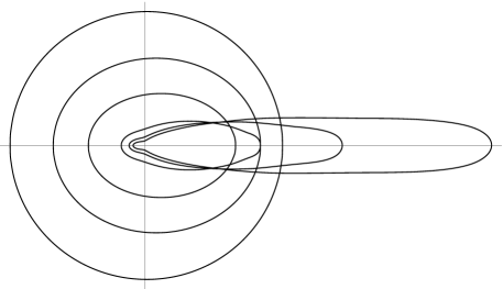
Figure 1: Anisotropy of photon distribution in the comoving reference frame developing near the photosphere. When the outflow has high optical depth the distribution is isotropic, but near the photosphere it becomes increasingly anisotropic. The direction of medium motion is to the right. The optical depth for these curves is $\tau=100,10,5,1.4,0.7,0.3$ with increasing anisotropy.

Our computation is performed in the comoving reference frame. In order to find the photon spectrum which a distant observer will detect we have to transform the spectrum into the laboratory reference frame. One has to use the following transformations

$$N(\epsilon_{L})=2\pi\int_{0}^{1}d\mu_{L}r^{2}\mu_{L}n(\epsilon,\mu))\epsilon_{L}^{2},$$ (10)

$$\epsilon=\Gamma(1-\beta\mu_{L})\epsilon_{L},\quad\quad\mu=\frac{\mu_{L}-\beta}{1-\beta\mu_{L}},$$ (11)

where the subscript ”$L$” denotes quantities in the laboratory frame.

Two asymptotic cases were found in Ruffini et al. (2013) to have very different spectra from the photosphere: photon thick and photon thin ones. Since the photon thin case is characterized by nearly Planck instantaneous observed spectrum, here we concentrate on the photon thick case.

Consider steady relativistic wind with the following parameters:

$$L=10^{54}\text{ erg/s, }\Gamma=500\text{, }R_{0}=10^{8}\text{ cm}\text{, }k=2/3.$$ (12)

Given these values we find for initial optical depth

$$\tau_{0}=\frac{\sigma_{\mathrm{T}}L}{4\pi m_{p}c^{3}R_{0}\Gamma}=2.2\times 10^{10},$$ (13)

where $\sigma_{\mathrm{T}}$ is the Thomson cross section, and initial temperature $T_{0}=1.2$ MeV. The photospheric radius is

$$R_{ph}=\frac{\tau_{0}}{2\Gamma^{2}}R_{0}=4.4\times 10^{12}\text{ cm.}$$ (14)

We start the computation at the beginning of the coasting phase with $R_{i}=5\times 10^{10}$ cm where the optical depth is $\tau_{i}\sim 10^{2}$ and compute the spectrum until it settles to a static solution in the laboratory reference frame well above the photospheric radius $R\gg R_{ph}$.

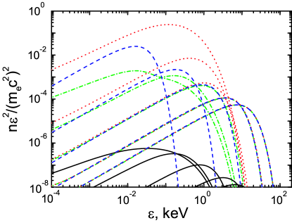
Figure 2: The spectrum of photons ($F_{\nu}$) in the comoving reference frame is shown for selected values of radii: $5\times 10^{10}$, $10^{11}$, $10^{12}$, $10^{13}$ and $5\times 10^{14}$ cm. Solid curves show integrated spectrum over angles, dashed curves show the Planck spectrum with the temperature following the relation (9) with $k=2/3$ for comparison. Dotted curves show the spectra for $\mu=1$ (photons propagating forward in the comoving frame) and dash-dotted curves correspond to $\mu=-1$ (photons propagating backward in the comoving frame).

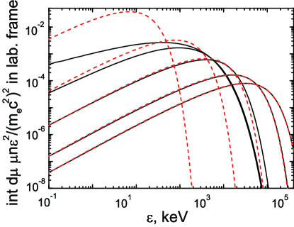
Figure 3: The spectrum of photons ($F_{\nu}$) transformed to the laboratory reference frame is shown for selected values of radii, corresponding to Fig. 2. Solid curves show the observed spectrum of photons integrated over angles, dashed curves show the spectrum of photons arriving to a given radius with thermal spectrum in the comoving reference frame, transformed to the laboratory reference frame.

In Fig. 2 we show the evolution of photon spectrum in comoving reference frame for selected values of radii starting at large optical depth through the photosphere ending up at small optical depth $\tau\sim 10^{-2}$.

While the spectrum in comoving frame initially keeps the Planck shape, it becomes distorted with decreasing optical depth. It is also the consequence of interaction with electrons which on average have smaller energy than photons do, see Fig. 2. In fact, near the photosphere the average energy of photons saturates Beloborodov (2011), but the one of electrons continues to decrease. When this spectrum is transformed to the laboratory frame using Eq. (11) we find increasing deviations from Planck spectrum essentially due to contribution from different angles. Clearly this effect becomes less and less prominent with decreasing optical depth. The final shape of the spectrum is reached for $\tau>10^{-2}$. Our results for the steady coasting relativistic wind agree quantitatively with those obtained by Bégué et al. (2013) and by Ruffini et al. (2013).

In Fig. 2 we also show the spectra of photons propagating forward (for which the angle $\theta$ between the momentum of the photon and the radius vector vanishes, dotted curve) and those propagating backward (for which $\theta=\pi$, dash-dotted curve). While photons propagating forward dominate in the spectrum due to Doppler effect, the contribution of photons with $\theta>0$ changes the shape of the spectrum compared to the black body one, especially near its peak.

We also computed observed spectrum with different values of $k$ parameter. The values of $k>2/3$ imply that the temperature in the wind decreases with radius faster than the one given by the steady solution. More rapid change of temperature with radius may mimic some more realistic profiles of finite radial extension of the outflow, see e.g. Piran et al. (1993). Photons propagating in such outflows scatter on electrons with lower temperature, which leads to additional comptonization of the spectrum. At large optical depths photon spectrum adjusts to the electron temperature. With decreasing optical depth only low energy part of the spectrum is affected by comptonization.

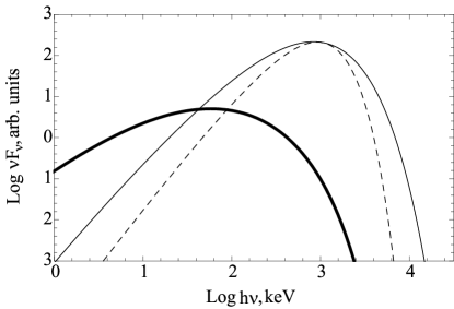
Figure 4: The final observed spectrum of photons ($\nu F_{\nu}$) is shown for two values of $k$ parameter: $k=2/3$ (thin curve) and $k=2$ (thick curve). For comparison Planck spectrum is shown by dashed curve.

In Fig. 4 we show for comparison two final observed spectra $\nu F(\nu)\propto n\epsilon^{4}$ with different values of $k$, namely $k=2/3$ and $k=2$. It is interesting to note that the number of photons in the low energy part of the spectrum increases with increasing $k$. This low energy part of the spectrum can be fit with a power law. Performing the fit in the energy range between 1 and 10 keV we found that the power law index changes as follows

$$\alpha\simeq 1-k.$$ (15)

This power law index $\alpha$ actually coincides with the one used in the Band phenomenological spectrum Band et al. (1993). Thus we find that Compton scattering near the photosphere can change the low energy part of observed spectrum. In particular, the photon index $\alpha$ is shown to depend on the index $k$ which parametrizes the electron temperature dependence on radius.

In our calculations the stationary wind model is used. The observed durations of GRBs range from a fraction of second to thousands of seconds, hence the finite duration effects have to be taken into account for theoretical calculations of light curves and spectra of the photospheric emission. Such finite duration effects give rise to a new classification of relativistic outflows, which is discussed in details by Ruffini et al. (2013), see also Bégué et al. (2013).

Besides one has to keep in mind that the prompt emission of GRBs contains not only photospheric component but in most cases also non-thermal component originating from optically thin regions of the outflow. However, unambiguous identification of the photospheric component in GRBs is crucial since it provides basic information about the physical parameters of GRBs, see e.g. Iyyani et al. (2013).

4 Conclusions

We considered relativistic steady wind and computed the observed spectrum of its photospheric emission. For this goal we solved the equation of radiative transfer in comoving reference frame with exact Compton collision term in Fokker-Planck approximation, including the effect of anisotropy of the photon field. We obtained the photon spectra in the laboratory frame, as seen by a distant observer.

We confirmed the result of Beloborodov (2011) indicating the presence of strong anisotropy developed in the comoving frame at the photosphere. Some qualitative differences in our results are due to the fact that he used approximate collision term, instead of our exact one.

The observed spectrum from the photosphere of the steady coasting relativistic wind is found in agreement with previous studies. We also found that when the temperature decreases with radius faster than in the case of a steady wind the low energy part of the observed spectrum changes significantly with respect to the Planck function. In particular, for the temperature profile $T\propto r^{-2}$ we found for the Band index $\alpha\simeq-1$, in agreement with typical low energy photon index observed in GRBs.

References

- Band et al. (1993) Band D., Matteson J., Ford L., Schaefer B., Palmer D., Teegarden B., Cline T., Briggs M., Paciesas W., Pendleton G., Fishman G., Kouveliotou C., Meegan C., Wilson R., Lestrade P., 1993, ApJ, 413, 281
- Bégué et al. (2013) Bégué D., Siutsou I. A., Vereshchagin G. V., 2013, ApJ, 767, 139
- Beloborodov (2010) Beloborodov A. M., 2010, MNRAS, 407, 1033
- Beloborodov (2011) Beloborodov A. M., 2011, ApJ, 737, 68
- Bianco et al. (2001) Bianco C. L., Ruffini R., Xue S., 2001, A&A, 368, 377
- Daigne & Mochkovitch (2002) Daigne F., Mochkovitch R., 2002, MNRAS, 336, 1271
- Fukue et al. (1985) Fukue J., Kato S., Matsumoto R., 1985, PASJ, 37, 383
- Giannios (2006) Giannios D., 2006, A&A, 457, 763
- Goodman (1986) Goodman J., 1986, ApJ, 308, L47
- Iyyani et al. (2013) Iyyani S., Ryde F., Axelsson M., Burgess J. M., Guiriec S., Larsson J., Lundman C., Moretti E., McGlynn S., Nymark T., Rosquist K., 2013, MNRAS, 433, 2739
- Levinson (2012) Levinson A., 2012, ApJ, 756, 174
- Mészáros et al. (2002) Mészáros P., Ramirez-Ruiz E., Rees M. J., Zhang B., 2002, ApJ, 578, 812
- Mészáros & Rees (2000) Mészáros P., Rees M. J., 2000, ApJ, 530, 292
- Nagirner et al. (1997) Nagirner D. I., Loskutov V. M., Grachev S. I., 1997, Astrophysics, 40, 227
- Paczynski (1986) Paczynski B., 1986, ApJ, 308, L43
- Paczynski (1990) Paczynski B., 1990, ApJ, 363, 218
- Pe’er (2008) Pe’er A., 2008, ApJ, 682, 463
- Pe’er & Ryde (2011) Pe’er A., Ryde F., 2011, ApJ, 732, 49
- Pe’er et al. (2007) Pe’er A., Ryde F., Wijers R. A. M. J., Mészáros P., Rees M. J., 2007, ApJ, 664, L1
- Piran et al. (1993) Piran T., Shemi A., Narayan R., 1993, MNRAS, 263, 861
- Psaltis & Lamb (1997) Psaltis D., Lamb F. K., 1997, ApJ, 488, 881
- Rees & Mészáros (2005) Rees M. J., Mészáros P., 2005, ApJ, 628, 847
- Ruffini et al. (2009) Ruffini R., Aksenov A. G., Bernardini M. G., Bianco C. L., Caito L., Chardonnet P., Dainotti M. G., de Barros G., Guida R., Izzo L., Patricelli B., Lemos L. J. R., Rotondo M., Hernandez J. A. R., Vereshchagin G., Xue S.-S., 2009, in Novello M., Perez S., eds, American Institute of Physics Conference Series Vol. 1132 of American Institute of Physics Conference Series, The Blackholic energy and the canonical Gamma-Ray Burst IV: the “long,” “genuine short” and “fake-disguised short” GRBs. pp 199–266
- Ruffini et al. (2001) Ruffini R., Bianco C. L., Fraschetti F., Xue S.-S., Chardonnet P., 2001, ApJ, 555, L113
- Ruffini et al. (2013) Ruffini R., Siutsou I. A., Vereshchagin G. V., 2013, ApJ, 772, 11
- Ryde et al. (2011) Ryde F., Pe’Er A., Nymark T., Axelsson M., Moretti E., Lundman C., Battelino M., Bissaldi E., Chiang J., Jackson M. S., Larsson S., Longo F., McGlynn S., Omodei N., 2011, MNRAS, 415, 3693
- Shemi & Piran (1990) Shemi A., Piran T., 1990, ApJ, 365, L55
- Toma et al. (2011) Toma K., Wu X.-F., Mészáros P., 2011, MNRAS, 415, 1663
- Vurm et al. (2013) Vurm I., Lyubarsky Y., Piran T., 2013, ApJ, 764, 143