Mechanisms in Environmentally-Assisted One-photon Phase Control

Abstract

The ability of an environment to assist in one-photon phase control relies upon entanglement between the system and bath and on the breaking of the time reversal symmetry. Here, one photon phase control is examined analytically and numerically in a model system, allowing an analysis of the relative strength of these contributions. Further, the significant role of non-Markovian dynamics and of moderate system-bath coupling in enhancing one-photon phase control is demonstrated, and an explicit role for quantum mechanics is noted in the existence of initial non-zero stationary coherences. Finally, desirable conditions are shown to be required to observe such environmentally assisted control, since the system will naturally equilibrate with its environment at longer times, ultimately resulting in the loss of phase control.

I Introduction

The coherent control of molecular processes as been highly successful, both computationally and experimentally, when applied to isolated molecular systems Shapiro and Brumer (2012). Indeed, a wide variety of scenarios has been proposed ranging from the control of products in the continuum, such as photodissociation, to bound state control of radiationless transitionsShu and Henriksen (2011, 2012); Grinev, Shapiro, and Brumer (2013) . By contrast, control of a system in the presence of an environment, where decoherence effects often destroy coherencesSchlosshauer (2007); Elran and Brumer (2013). is only in its early stages of development. To this end, one photon phase control, the subject of this paper, is of particular interest insofar as the environment assists, rather than impedes, control of the system dynamics.

One photon phase control has been the subject of considerable recent discussion and attention Prokhorenko et al. (2006); Joffre (2007); Prokhorenko et al. (2007); Florean et al. (2009); Katz, Ratner, and Kosloff (2010); Spanner, Arango, and Brumer (2010); Kosloff et al. (2011); Prokhorenko et al. (2011); General Disucssion (2011); Arango and Brumer (2013); Pachón, Yu, and Brumer (2013). In this one photon phase control (OPPC) scenario, control is achieved by varying the spectral phase of a weak pulse while keeping its power spectrum fixed. Particular interest in this scenario arises from a seminal proof in which it was shown that OPPC was not possible for isolated molecular systems in which control was over products in the continuumBrumer and Shapiro (1989). However, subsequent experiments on control of retinal isomerization in bacteriorhodopsin in the weak regimeProkhorenko et al. (2006) as well as in the strong field regimeFlorean et al. (2009) motivated controversyJoffre (2007); Prokhorenko et al. (2007); Florean et al. (2009); Prokhorenko et al. (2011) and the need for clarification of conditions under which such control was possible.

This clarification, provided in Refs. 12 and 17, showed that control was possible for both isolated systems and open quantum systems under well defined conditions. In particular, for an observable $\hat{O}$ of a physicochemical system defined by the Hamiltonian $\hat{H}_{\mathrm{S}}$, it was shown that: (i) if the system is isolated and initially devoid of coherence then one-photon phase control is possible only if $[\hat{H}_{\mathrm{S}},\hat{O}]\neq 0$, but (ii) if the system is coupled to an environment, as in any realistic case, then control is possible not only if $[\hat{H}_{\mathrm{S}},\hat{O}]\neq 0$, but even if $[\hat{H}_{\mathrm{S}},\hat{O}]=0$, in which case it is environmentally assistedSpanner, Arango, and Brumer (2010); Arango and Brumer (2013); Pachón, Yu, and Brumer (2013). As it was noted in Refs. 12 and 17, the case of $[\hat{H}_{\mathrm{S}},\hat{O}]\neq 0$ includes, e.g., isomerization since the probability of observing an isomer is an observable that does not commute with $\hat{H}_{\mathrm{S}}$.

The aim of Ref. 12 was to establish these general commutation-based rules, whereas Ref. 17 identified the physical processes responsible for OPPC. In particular, based on a general master equation approach, we qualitatively identified two main mechanisms for OPPC in open systems: the breaking of time-reversal symmetry and the entanglement between the system and the bath. These two mechanisms differ in character; the time-reversal symmetry does not rely upon quantum mechanics, whereas the initial correlations between the system and the bath are quantum in naturePachón, Triana, and Brumer (2013). These mechanisms also work on different time scales, the initial correlations contribute in the short time regime while the time-reversal symmetry dominates in the long time regime. As such, it is the latter that determines the amount of control that can be achieved within this control scheme.

In this paper, we quantitative analyze the magnitude of each of these contributions and demonstrate the significant role of the non-Markovian dynamics and of moderate system-bath coupling in enhancing the extent of one-photon phase control. Note that the system-bath interaction plays a dual role in the OPPC scenario. First, it assists insofar as allowing phase control for systems where such control would not occur if the system were isolated. However, since the system-bath coupling persists long after the laser pulse, it induces relaxation to equilibrium at long times, resulting in long-time loss of phase control. Hence, as we show below, maintaining phase control over an extended period of time requires careful balancing of the system-bath interactions.

II Initial considerations

Consider a quantum system S described by the Hamiltonian $\hat{H}_{\mathrm{S}}$ with $\hat{H}_{\mathrm{S}}|\,n\,\rangle=E_{n}|\,n\,\rangle$. We consider below two cases, where the system is isolated and irradiated with a laser, and the second where the system is irradiated in the presence of an environment (or “bath”). In the latter case, the full Hamiltonian is given by $\hat{H}=\hat{H}_{\mathrm{S}}+\hat{V}_{\mathrm{L}}+\hat{H}_{\mathrm{B}}+\hat{H}_{\mathrm{SB}}$, where $\hat{V}_{\mathrm{L}}$ denotes the term laser, $\hat{H}_{\mathrm{B}}$ is the Hamiltonian of the environment and $\hat{H}_{\mathrm{SB}}$ is the system-bath coupling.

II.1 Initial Considerations on System Dynamics

Under the influence of time-dependent fields and in the presence of an environment, the time evolution of the system density-operator $\hat{\rho}_{\mathrm{S}}$ is given by Pachón and Brumer (2013a)

$$\begin{split}\langle n|\hat{\rho}_{\mathrm{S}}(t)|m\rangle&=\sum_{\nu}J_{nm;\nu\nu}(t)\langle\nu|\hat{\rho}_{\mathrm{S}}(0)|\nu\rangle\\ &+\sum_{\nu\neq\mu}J_{nm;\nu\mu}(t)\langle\nu|\hat{\rho}_{\mathrm{S}}(0)|\mu\rangle,\end{split}$$ (1)

where $J_{nm;\nu\mu}(t)$ denotes the propagation function in the system energy basis representation Pachón and Brumer (2013a). As such, the system dynamics is contained in the propagation function elements $J_{nm;\nu\mu}(t)$ that can be derived, as in Ref. 20, from a path integral representation of the propagation function. The first two indices $nm$ denote the density matrix element in which we are interested and the last two indices $\nu\mu$ refer to the elements of the initial density matrix that contribute, as shown in Eq. (1), to the dynamics of the $nm$-th element. The general picture implied by Eq. (1) is that the time evolution of the diagonal elements $n=m$ (populations) as well as the off-diagonal elements (coherences) of the density matrix depends linearly on the initial diagonal and off-diagonal elements.

To explore the physical meaning and role of the $J_{nm;\nu\mu}(t)$ consider first the case of unitary time-evolution in absence of time dependent external forces. Examining this case allows a reinterpretation of some of the known features of unitary dynamics in terms of this formalism. In the case of unitary time-evolution, the elements of the propagating function in Eq. (1) reduce to the familiar expression

$$J_{nm;\nu\mu}(t)=\mathrm{e}^{-\mathrm{i}(E_{m}-E_{n})t/\hbar}\delta_{n\nu}\delta_{m\mu}.$$ (2)

The Kronecker deltas prevent (a) the transfer of initial population from $\langle\,\nu\,|\hat{\rho}_{\mathrm{S}}(0)|\,\nu\,\rangle$ to $\langle\,n\,|\hat{\rho}_{\mathrm{S}}(t)|\,n\,\rangle$ mediated by $J_{nn;\nu\nu}(t)$, as well as (b) the generation of coherences, $n\neq m$, from initial populations $\langle\nu|\hat{\rho}_{\mathrm{S}}(0)|\nu\rangle$. In addition, the possibility of controlling the populations at time $t$, i.e., the $\langle n|\hat{\rho}_{\mathrm{S}}(t)|n\rangle$, by varying the initial coherences $\langle\nu|\hat{\rho}_{\mathrm{S}}(0)|\mu\rangle$, $\nu\neq\mu$, a possible control objective, is also prevented during the unitary time evolution governed by Eq. (2).

In the presence of time dependent external fields or of an external environment, the propagating function elements $J_{nm;\nu\mu}(t)$ differ from those in Eq. (2), as discussed below. Although the particular form of the $J_{nm;\nu\mu}(t)$ depends upon the environment and on the external field, generally the Kronecker delta restrictions will disappear, allowing for the transfer of population, the generation of coherences and the contribution of the initial coherences to the time evolution of the populations. Specifically, in the presence of dissipation, the delta functions in Eq. (2) broaden, allowing for the additional processes discussed below. In Ref. 20 we provide a deeper description of these extra processes in the context of incoherent excitation of open quantum systems Jiang and Brumer (1991); Hoki and Brumer (2011); Brumer and Shapiro (2012); Pachón and Brumer (2013b, a). These effects are quantitatively considered, for OPPC, below.

II.2 Initial Considerations on Control

Consider now controlling the expectation value of a system observable $\hat{O}$. In general, the time evolution of the expectation value $\hat{O}$ can be expressed as $\langle\hat{O}(t)\rangle=\sum_{n,m}\langle n|\hat{O}|m\rangle\langle m|\hat{\rho}_{\mathrm{S}}(t)|n\rangle.$ We are particularly interested in observables where $[\hat{O},\hat{H}_{\mathrm{S}}]=0$, i.e. those that are not phase controllable Spanner, Arango, and Brumer (2010); Pachón, Yu, and Brumer (2013) in isolated systems. In this case, $\langle\hat{O}(t)\rangle=\sum_{n}\langle n|\hat{O}|n\rangle\langle n|\rho_{\mathrm{S}}(t)|n\rangle.\,$Using Eq. (1), we obtain

$$\begin{split}\langle\hat{O}(t)\rangle&=\sum_{n,\nu}\langle n|\hat{O}|n\rangle J_{nn;\nu\nu}(t)\langle\nu|\hat{\rho}_{\mathrm{S}}(0)|\nu\rangle\\ &+\sum_{n,\nu\neq\mu}\langle n|\hat{O}|n\rangle J_{nn;\nu\mu}(t)\langle\nu|\hat{\rho}_{\mathrm{S}}(0)|\mu\rangle.\end{split}$$ (3)

First consider one-photon phase control from states initially devoid of coherence, i.e., $\langle\nu|\hat{\rho}_{\mathrm{S}}(0)|\mu\rangle=0$ for $\nu\neq\mu$. Under these circumstances, and with the assumption of irradiation with weak laser fields, one-photon phase control is not possible if the molecule is isolated, i.e., if the dynamics is unitarySpanner, Arango, and Brumer (2010); Pachón, Yu, and Brumer (2013). By contrast, for the case of non-unitary dynamics (the open system case), environmentally assisted control is possibleSpanner, Arango, and Brumer (2010); Pachón, Yu, and Brumer (2013).

Below, we examine the origin and nature of this effect. Although Eq. (3) is general, we anticipate two physical mechanisms that could be responsible for one-photon phase control in the open-system case. The first arises from the fact that, in the presence of the environment, the stationary states of the system are no longer diagonal in the system’s Hamiltonian eigenbasis $\{|\,n\,\rangle\}$. Specifically, interaction with the environment produces off-diagonal elements in the initial system density operator $\hat{\rho}_{\mathrm{S}}(0)$ which, by virtue of Eq. (3), will contribute to the evolution of the expectation value of $\hat{O}$. The second relates to time-reversal-symmetry breaking. For unitary evolution, one can decompose $J_{nn;\nu\nu}(t)$ into two terms, one related to the process $|\,\nu\,\rangle\rightarrow|\,n\,\rangle$ and another term related to the dual process, $\langle\,n\,|\leftarrow\langle\,\nu\,|$. These two processes “interfere destructively” in $J_{nn;\nu\nu}(t)$. However, in the particular case of an open system this symmetry is broken, allowing for the encoding of phase information in $J_{nn;\nu\nu}(t)$, as noted below.

A detailed analysis of phase control in an isolated and model system follows below.

III Unitary Evolution and One-photon Phase-control

To examine one-photon phase control we consider an analytically soluble model for both the unitary and non-unitary cases. In particular, consider the vibrations of a diatomic molecule of frequency $\omega_{0}=\sqrt{k/m}$, where $m$ is the reduced mass and $k$ the coupling constant between the atoms. Although an apparently simple model, it will be seen to provide great insight into the physics of phase control. It also provides a model for a wide variety of physical systems such as nano-mechanical resonators, trapped ions, membranes, optical mirrors, etc. Galve, Pachón, and Zueco (2010).

For the unitary case, the Hamiltonian is given by

$$\begin{split}\hat{H}&=\hat{H}_{\mathrm{S}}+\hat{V}_{\mathrm{L}}=\frac{\hat{p}^{2}}{2m}+\frac{m\omega_{0}^{2}}{2}\hat{q}^{2}+\hat{q}E(t),\end{split}$$ (4)

where $E(t)$ denotes the electric field of the laser pulse. This Hamiltonian describes then a linearly-forced harmonic oscillator. The Fourier transform of the electric field is $\tilde{E}(\omega)=\sqrt{|S(\omega)|}\exp[-{\rm i}\varphi(\omega)]$, where $S(\omega)$ is the field amplitude and $\varphi(\omega)$ is the spectral phase. “Phase control” refers to the effects on the molecular dynamics of manipulating the spectral phase $\varphi(\omega)$, while keeping $S(\omega)$ fixed.

III.1 System Unitary Time Evolution

In the position representation, the time evolution of the system-density-matrix element $\rho_{\mathrm{S}}(\mathbf{q}^{\prime},0)=\langle\,q_{+}^{\prime}\,|\hat{\rho}_{\mathrm{S}}(0)|\,q_{-}^{\prime}\,\rangle$ can derived from

$$\begin{split}\rho_{\mathrm{S}}(\mathbf{q}^{\prime\prime},t)=\int\mathrm{d}q^{\prime}J(\mathbf{q}^{\prime\prime},t;\mathbf{q}^{\prime},0)\rho_{\mathrm{S}}(\mathbf{q}^{\prime},0),\end{split}$$ (5)

where $J(\mathbf{q}^{\prime\prime},t;\mathbf{q}^{\prime},0)$ is the propagating function, which for the case of unitary time-evolution is $J(\mathbf{q}^{\prime\prime},t;\mathbf{q}^{\prime},0)=U(q_{+}^{\prime\prime},q_{+}^{\prime},t)U^{*}(q_{-}^{\prime\prime},q_{-}^{\prime},t)$, with $U(q_{+}^{\prime\prime},q_{+}^{\prime},t)=\langle\,q_{+}^{\prime\prime}\,|\hat{U}(t)|\,q_{+}^{\prime}\,\rangle$ and $\hat{U}(t)=\hat{\mathcal{T}}\exp[-\mathrm{i}\int_{t_{0}}^{t}\mathrm{d}s\hat{H}(s)/\hbar]$, $\hat{\mathcal{T}}$ being the time-ordering operator Feynman and Hibbs (1965); Ingold (2002); Pachón, Ingold, and Dittrich (2010). For the unitary case, with time evolution operator $\hat{U}(t)$, one can obtain the propagating function elements $J_{nm;\nu\mu}(t)$ in Eq. (1) by projecting onto the system energy basis Pachón and Brumer (2013a). For the particular case in Eq. (4), the unitary time evolution can be obtained analytically (c.f. Chap. 3 in Ref. 26 or Chap. 2 in Ref. 27), giving analytic propagating function elements.

For the purpose of discussion, consider the case where the system is prepared in a coherent superposition of the ground and first excited states, i.e., $\hat{\rho}_{\mathrm{S}}(0)=\left(|\,0\,\rangle\langle\,0\,|+|\,0\,\rangle\langle\,1\,|+|\,1\,\rangle\langle\,0\,|+|\,1\,\rangle\langle\,1\,|\right)/2$. From Eq. (3), we have

$$\langle\hat{O}(t)\rangle=\frac{1}{2}\sum_{\begin{subarray}{c}n\\ \nu,\mu=0,1\end{subarray}}\langle n|\hat{O}|n\rangle J_{nn;\nu\mu}(t),$$ (6)

where

$$\begin{split}J_{nn;00}(t)&=\frac{1}{n!\mathcal{E}_{0}^{2n}}|\mathcal{E}(t)|^{2n}\exp\left\{-\frac{|\mathcal{E}(t)|^{2}}{\mathcal{E}_{0}^{2}}\right\},\end{split}$$ (7)

$$\begin{split}J_{nn;01}(t)&=\frac{1}{n!{\mathcal{E}_{0}}^{2n+1}}|\mathcal{E}(t)|^{2n-2}\exp\left\{-\frac{|\mathcal{E}(t)|^{2}}{\mathcal{E}_{0}^{2}}\right\}\\ &\times\mathcal{E}(t)\left\{-2n\mathcal{E}_{0}^{2}+|\mathcal{E}(t)|^{2}\right\},\end{split}$$ (8)

$$\begin{split}J_{nn;11}(t)&=\frac{1}{n!{\mathcal{E}_{0}}^{2n+2}}|\mathcal{E}(t)|^{2n-2}\exp\left\{-\frac{|\mathcal{E}(t)|^{2}}{\mathcal{E}_{0}^{2}}\right\}\\ &\times\left\{n^{2}\mathcal{E}_{0}^{4}+|\mathcal{E}(t)|^{2}\left[-2n\mathcal{E}_{0}^{2}+|\mathcal{E}(t)|^{2}\right]\right\},\end{split}$$ (9)

$J_{nn;10}(t)=J_{nn;01}^{*}(t)$, $\mathcal{E}_{0}=\sqrt{2m\omega_{0}\hbar}$, and

$$\mathcal{E}(t) =E_{-}^{2}(t)+2\cos(\omega_{0}t)E_{-}(t)E_{+}(t)+E_{+}^{2}(t)$$ (10)

$$=\int_{-\infty}^{t}\mathrm{d}s\exp(-{\rm i}s\omega_{0})E(s).$$ (11)

For later convenience, we have defined $E_{+}(t)=\int_{-\infty}^{t}\mathrm{d}sE(s)G_{+}(t-s)/G_{+}(t),$ and $E_{-}(t)=\int_{-\infty}^{t}\mathrm{d}sE(s)G_{-}(s)/G_{-}(t),$ where $G_{\pm}(s)$ denotes the inverse Laplace transform of $\hat{G}_{\pm}(z)=\left(z^{2}+\omega_{0}^{2}\right)^{-1}$. The specific combination of $E_{+}(t)$ and $E_{-}(t)$ in Eq. (10) is responsible for the simple result in Eq. (11). As shown below, this precise form is lost in the open system case giving rise to phase control. In the following, we use linearly chirped laser pulses

$$E(t)=E_{0}\mathrm{e}^{-4\left(\frac{t-t_{0}}{\Delta t}\right)^{2}}\cos\left[\Omega_{\mathrm{L}}(t-t_{0})+\chi(t-t_{0})^{2}\right],$$ (12)

where $t_{0}$ and $\Delta t$ are the center and width of the Gaussian pulse envelope, $E_{0}$ and $\Omega_{\mathrm{L}}$ are the field strength and carrier frequency of the laser with chirp rate $\chi$. Changing the sign of $\chi$ causes a change in the laser phase while retaining the intensity profile.

In the long time regime, $t\rightarrow\infty$, $\mathcal{E}(t)$ becomes the Fourier transform of the field $E(t)$. This implies that the term $|\mathcal{E}(t)|$ does not contain any information about the spectral phase. Hence, here, laser phase information is not encoded in either $J_{nn;00}(t)$ or $J_{nn;11}(t)$, but only in $J_{nn;01}(t)$. Thus, if the initial state is an incoherent superposition of $|\,0\,\rangle$ and $|\,1\,\rangle$ then the expectation value of $\hat{O}$ does not depend on the phase function $\varphi(\omega)$. This result makes no reference to the field strength, but is a particularity of the chosen system which is not expected to be true in general.

In order to make a connection with the general weak field results derived in Refs. 12 and 17, we consider Eqs. (7)-(9) in the weak field regime, $\sqrt{|S(\omega_{0})|}/\mathcal{E}_{0}\ll 1$, to get:

$$J_{00;00} (\infty)=1-J_{00;11}(\infty),$$ (13)

$$J_{00;10} (\infty)=\frac{1}{\mathcal{E}_{0}}\int_{-\infty}^{\infty}\mathrm{d}s\,\mathrm{e}^{-\mathrm{i}\omega_{0}s}E(s),$$ (14)

$$J_{00;11} (\infty)=\frac{1}{\mathcal{E}_{0}^{2}}\left|\int_{-\infty}^{\infty}\mathrm{d}s\,\mathrm{e}^{-\mathrm{i}\omega_{0}s}E(s)\right|^{2}.$$ (15)

These expressions correspond to the typical results in lowest order perturbation theory in the field amplitude Shapiro and Brumer (2003). Clearly, phase dependence is not manifest in the long-time diagonal terms $J_{00;00}(\infty)$ or $J_{00;11}(\infty)$. Sample results are shown in Fig. 1, it is clear that no phase dependence is present after the pulse is over. Hence, the long time regime is defined as after the pulse is over. As discussed below, this is no longer the case when environmental effects are considered.

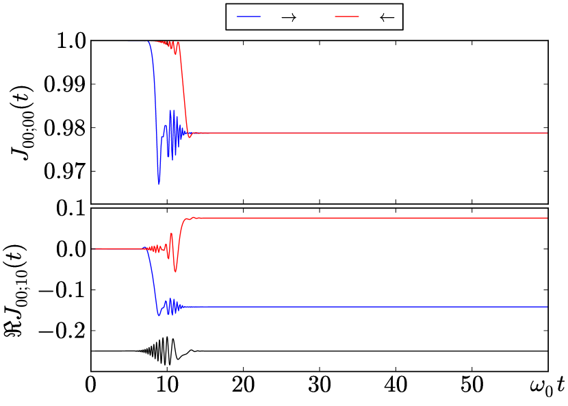
Figure 1: Phase dependence in unitary dynamics. $J_{00;00}(t)$ (upper panel) and $J_{00;10}(t)$ (lower panel) induced by the chirped pulse in Eq. (12) with $\omega_{0}t_{0}=10$, $\Omega_{\mathrm{L}}=10\omega_{0}$, $\Delta t\omega_{0}=4$ and $\sqrt{|S(\omega_{0})|}/\mathcal{E}_{0}=0.003415$ with $\chi=2.5$ [($\rightarrow$) dark blue curve] and $\chi=-2.5$ [($\leftarrow$) light red curve]. For reference, we have added at the bottom of the lower panel the laser pulse as a function of time (black curve).

Interestingly, for this particular case, the weak field condition $\sqrt{|S(\omega_{0})|}/\mathcal{E}_{0}=\sqrt{|S(\omega_{0})|}/\sqrt{2m\hbar\omega_{0}}\ll 1$ implies that, for the same value of $\sqrt{|S(\omega_{0})|}$, one could be in a weak or strong field regime depending on the coupling constant ($k=m\omega_{0}^{2}$) and on the mean level spacing $\hbar\omega_{0}$.

IV Non-unitary evolution and One-photon Phase-control

Consider then the case of dynamics and control in an open system. We treat the dissipative dynamics using the influence functional approach Feynman and Vernon (1963). The starting condition is obtained by coupling the central system S to an external system B which is represented by an infinite number of freedoms Feynman and Vernon (1963). This system B can be, e.g., a thermal bath, the vibrational modes of a molecular complex, blackbody radiation, etc. The Hamiltonian of the the system S plus B can be written as

$$\hat{H}=\hat{H}_{\mathrm{S}}+\hat{H}_{\mathrm{B}}+\hat{H}_{\mathrm{SB}}+\hat{V}_{\mathrm{L}}$$ (16)

where $\hat{H}_{\mathrm{S}}+\hat{V}_{\mathrm{L}}$ are given in Eq. (4), $\hat{H}_{\mathrm{B}}$ is the Hamiltonian of the thermal bath and $\hat{H}_{\mathrm{SB}}$ describes the interaction of the system with B. We assume that system B is composed of a collection of harmonic oscillators with masses $m_{j}$, frequencies $\omega_{j}$ and coupled linearly to S with constant couplings $c_{j}$ Caldeira and Leggett (1983); Grabert, Schramm, and Ingold (1988); Weiss (2012).

After tracing over the environment the influence of the bath on the time evolution of the system S is described via the spectral density $J(\omega)$, given by Caldeira and Leggett (1983); Grabert, Schramm, and Ingold (1988); Weiss (2012) $J(\omega)=\pi\sum_{j=1}^{\infty}\frac{c_{j}^{2}}{2m_{j}\omega_{j}}\delta(\omega-\omega_{j}).$ Once $J(\omega)$ is fixed, one can express the relaxation process by means of the dissipative kernel $\gamma(s)=\frac{2}{m}\int_{0}^{\infty}\frac{\mathrm{d}\omega}{\pi}\frac{J(\omega)}{\omega}\cos(\omega s)$, while the decoherence process induced by thermal fluctuations can be described by the decoherence kernel $K^{\prime}(s)=\int_{0}^{\infty}\frac{\mathrm{d}\omega}{\pi}J(\omega)\mathrm{coth}\left(\frac{\hbar\beta\omega}{2}\right)\cos(\omega s).$ Here $\beta=1/k_{\mathrm{B}}T$ and $T$ denotes the temperature of the thermal bath.

Below, we primarily employ the most commonly used spectral density, the Ohmic spectral density with a finite Drude cutoff $\omega_{\mathrm{D}}$,

$$J_{\mathrm{Ohm}}(\omega) =m\gamma\omega\,\omega_{\mathrm{D}}^{2}/\left(\omega^{2}+\omega_{\mathrm{D}}^{2}\right),$$ (17)

where $\gamma$ is the strength coupling constant to the thermal bath. This spectral density generates the dissipative kernel $\gamma(s)=\gamma\omega_{\mathrm{D}}\exp\left(-\omega_{\mathrm{D}}|t|\right)$. In the limit when the cutoff frequency $\omega_{\mathrm{D}}$ tends to infinity, $\gamma(s)\rightarrow 2\gamma\delta(s)$, corresponding to Ohmic dissipation.

IV.1 Description of the Initial State

Often, the initial state of S + B is assumed to be uncorrelated product Feynman and Vernon (1963); Caldeira and Leggett (1983), i.e. $\hat{\rho}_{\mathrm{S+B}}=\hat{\rho}_{\mathrm{S}}\otimes\hat{\rho}_{\mathrm{B}}$. However, this is not a sensible approximationGrabert, Schramm, and Ingold (1988) since it implies that system-bath interaction is turned on suddenly when the observation begins. In the absence of a specific initial system preparation, the most likely initial state for S+B is thermal. In this case if the coupling to the environment is strong, then the equilibrium state is given by Grabert, Schramm, and Ingold (1988) $\hat{\rho}_{\mathrm{S},\beta}=Z^{-1}_{\beta}\mathrm{tr}_{\mathrm{B}}\exp\left[-\left(\hat{H}_{\mathrm{S}}+\hat{H}_{\mathrm{B}}+\hat{H}_{\mathrm{SB}}\right)\beta\right],$ where $Z_{\beta}$ is the total partition function and tr_B denotes a trace over the bath.

For our particular case, $\hat{\rho}_{\mathrm{S},\beta}$ can be expressed analytically in terms of the effective Hamiltonian Grabert, Weiss, and Talkner (1984); Haake and Reibold (1985); Pachón, Triana, and Brumer (2013) $\hat{H}_{\mathrm{eff}}=\frac{1}{2m_{\mathrm{eff}}}\hat{p}^{2}+\frac{1}{2}m_{\mathrm{eff}}\omega_{\mathrm{eff}}^{2}\hat{q}^{2},$ with effective mass $m_{\mathrm{eff}}=\omega_{\mathrm{eff}}^{-1}\sqrt{\langle p^{2}\rangle\langle q^{2}\rangle^{-1}},$ and effective frequency $\omega_{\mathrm{eff}}=2(\hbar\beta_{\mathrm{TB}})^{-1}\mathrm{arccoth}\left(\frac{2}{\hbar}\sqrt{\langle p^{2}\rangle\langle q^{2}\rangle}\right),$ being $\langle q^{2}\rangle=\mathrm{tr}_{\mathrm{S}}(\hat{q}^{2}\hat{\rho}_{\mathrm{S},\beta})$ and $\langle p^{2}\rangle=\mathrm{tr}_{\mathrm{S}}(\hat{p}^{2}\hat{\rho}_{\mathrm{S},\beta})$, the equilibrium second momentsGrabert, Weiss, and Talkner (1984); Grabert, Schramm, and Ingold (1988). This $\hat{H}_{\mathrm{eff}}$ definition allows us to express $\hat{\rho}_{\mathrm{S},\beta}$ as

$$\hat{\rho}_{\mathrm{S},\beta}=Z_{\beta}^{-1}\sum_{n=0}^{\infty}\exp(-E_{n_{\beta}}\beta_{\mathrm{TB}})|n_{\beta}\rangle\langle n_{\beta}|,$$ (18)

where $\{E_{n_{\beta}}=\hbar\omega_{\mathrm{eff}}(n+\frac{1}{2})\}$ are the eigenvalues and $\{|n_{\beta}\rangle\}$ the eigenstates of the effective Hamiltonian $\hat{H}_{\mathrm{eff}}$. At high temperature, $\hbar\omega_{0}\beta\ll 1$ and $\frac{1}{2}\hbar\gamma\beta\ll 1$, $m_{\mathrm{eff}}$ and $\omega_{\mathrm{eff}}$ approach their bare values $m$ and $\omega_{0}$, respectively and, therefore, $\hat{\rho}_{\mathrm{S},\beta}$ approaches the canonical distributionGrabert, Weiss, and Talkner (1984); Hänggi and Ingold (2005); Pachón, Triana, and Brumer (2013). By contrast, at low temperatures $\hbar\omega_{0}\beta\gg 1$ and $\frac{1}{2}\hbar\gamma\beta\gg 1$, $m_{\mathrm{eff}}$ and $\omega_{\mathrm{eff}}$ deviate from the bare values $m$ and $\omega_{0}$ due to dampingGrabert, Weiss, and Talkner (1984); Hänggi and Ingold (2005); Pachón, Triana, and Brumer (2013). This deviation from the canonical distribution implies that the initial equilibrium state [Eq. (18)] contains stationary off-diagonal elements when it is projected on the eigenbasis of $\hat{H}_{\mathrm{S}}$. Note further that these off-diagonal elements are expected to vanish in classical mechanicsCampisi, Talkner, and Hänggi (2009). Hence, the existence of these terms is a purely quantum mechanical.

In order to explore the strength of the off-diagonal elements introduced in Eq. (18), we show, in Fig. 2, the matrix element $\langle 0|\hat{\rho}_{\mathrm{S},\beta}|2\rangle$ as a function of the coupling constant $\gamma$ and temperature $T$ for the non-Markovian regime, $\omega_{\mathrm{D}}=\omega_{0}$ (upper panel) and for the Markovian regime, $\omega_{\mathrm{D}}=100\omega_{0}$ (lower panel). In both cases, for fixed $\gamma$ the matrix element $\langle 0|\hat{\rho}_{\mathrm{S},\beta}|2\rangle$ is larger at low temperatures, whereas for fixed temperature it is larger for larger coupling constant $\gamma$. From Fig. (2) one can also see that the larger the cutoff $\omega_{\mathrm{D}}$, the larger the matrix element $\langle 0|\hat{\rho}_{\mathrm{S},\beta}|2\rangle$ at fixed $\gamma$ and $T$. This is consistent with the fact that the more Markovian the system, the larger is the decay rate, and therefore the larger the effective coupling to the bath (for an extended discussion on this parameter dependence see Ref. 19).

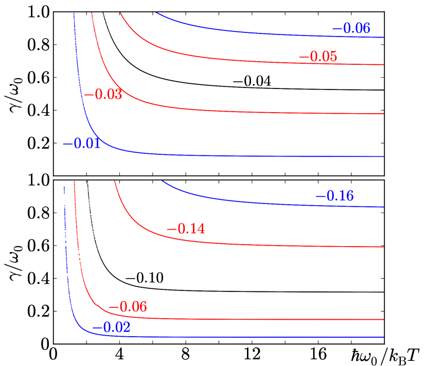
Figure 2: Stationary coherence generated by the Ohmic spectral density. Contours of constant matrix element $\langle 0|\hat{\rho}_{\mathrm{S},\beta}|2\rangle$ as a function of $\gamma$ and $T$ for fixed $\omega_{\mathrm{D}}=\omega_{0}$ (upper panel) and for $\omega_{\mathrm{D}}=100\omega_{0}$ (lower panel).

Note that increasing the value of $\langle 0|\hat{\rho}_{\mathrm{S},\beta}|2\rangle$ would imply a stronger contribution of these off-diagonal terms to the subsequent dynamics. However, in general, it would also imply fast relaxation, and therefore very fast loss of phase information. That is, coupling of the system to the bath plays two roles in phase control, one to enhance the phase control and one to cause relaxation. Below, in order to explicitly explore the system time-evolution and elucidate the contributions to phase control, we choose a moderate coupling constant, $\gamma=0.1\omega_{0}$ and low temperature $\hbar\omega_{0}/k_{\mathrm{B}}T=40$.

IV.2 Effect of the Initial Correlations

Based on the discussion for the unitary case, one can identify the deviations from the canonical distribution, and the related presence of off-diagonal elements in the initial density matrix, as the first contribution of the bath to one photon phase control. This implies that when laser excitation takes place, it finds off-diagonal elements of $\hat{\rho}_{\mathrm{S}}$, where laser phase information could be encoded (see below). This contribution occurs then on the time scale of the laser fieldPachón, Yu, and Brumer (2013).

Before considering the time evolution of the off-diagonal elements, it is useful to consider which of these terms are non-zero. From the symmetry of the resulting equilibrium state [see Eq. (18)], we expect the non-vanishing off-diagonal elements $\langle n|\hat{\rho}_{\mathrm{S},\beta}(0)|m\rangle$ that satisfy: $\mathrm{parity}(\langle n|q\rangle)\times\mathrm{parity}(\langle q|m\rangle)=\mathrm{even}$; this is the case in, e.g., $\langle 0|\hat{\rho}_{\mathrm{S},\beta}(0)|2\rangle$ or $\langle 1|\hat{\rho}_{\mathrm{S},\beta}(0)|3\rangle$. Hence, the bath is not able to induce stationary off-diagonal elements such as $\langle 0|\hat{\rho}_{\mathrm{S},\beta}(0)|1\rangle$ or $\langle 1|\hat{\rho}_{\mathrm{S},\beta}(0)|2\rangle$. Although a formal analysis of this fact could be carried out on the basis of the transitions induced by the bath after being traced out, for our proposes it suffices to consider this result as a consequence of the symmetries of the equilibrium state. Note that a similar analysis needs to be carried out for each particular system.

To demonstrate the phase dependence due to the stationary coherences in our model system, consider the propagating function element responsible for the $\langle 0|\hat{\rho}_{\mathrm{S}}(0)|2\rangle=\langle 0|\hat{\rho}_{\mathrm{S},\beta}|2\rangle$ to the time-evolution of the ground state $\langle 0|\hat{\rho}_{\mathrm{S}}(t)|0\rangle$,

$$\begin{split}J_{00;20}&(t)=\sqrt{\frac{8\pi^{2}}{q_{0}^{8}\hbar^{4}\det\mathsf{M}}}\frac{1}{N(t)}\mathrm{e}^{\frac{1}{2}\mathsf{E}^{\mathrm{T}}\mathsf{A}\mathsf{E}}\left\{(\mathsf{A}_{33}-q_{0}^{2})\hbar^{2}\right.\\ &\left.-2\left[(\mathsf{A}_{13}-\mathsf{A}_{23})E_{-}(t)(\mathsf{A}_{33}-\mathsf{A}_{34})\right]^{2}E_{+}(t)\right\},\end{split}$$ (19)

where $q_{0}=\sqrt{\hbar/m\omega_{0}}$, $N(t)=2\pi\hbar\frac{1}{m}|G_{+}(t)|\sqrt{2\pi\langle\hat{q}^{2}\rangle}$, and $\mathsf{E}=\left(E_{+}(t),E_{-}(t)\right)$ with $E_{+}(t)=\int_{0}^{t}\mathrm{d}sE(s)G_{+}(t-s)/G_{+}(t),$ $E_{-}(t)=\int_{0}^{t}\mathrm{d}sE(s)G_{-}(s)/G_{-}(t).$ Here $G_{+}(s)$ denotes the inverse Laplace transform of $G(z)=\left(z^{2}+z\gamma(z)+\omega_{0}^{2}\right)^{-1}$, being $\gamma(z)$ the Laplace transform of the dissipative kernel $\gamma(s)$ Grabert, Schramm, and Ingold (1988). $G_{-}(s)$ is related to $G_{+}(s)$ by means of the relation $\frac{G_{-}(s)}{G_{-}(t)}=\dot{G}_{+}(t-s)-\frac{G_{+}(t-s)}{G_{+}(t)}\dot{G}_{+}(s)$. As required, in the limit of vanishing coupling to the bath $\gamma\rightarrow 0$, $G_{+}(s)=G_{-}(s)=\frac{1}{2\mathrm{i}\omega_{0}}\left[\exp(\lambda_{1}t)-\exp(\lambda_{2}t)\right]$ with $\lambda_{1,2}=\pm\mathrm{i}\omega_{0}$ and $\mathsf{E}^{\mathrm{T}}\mathsf{A}\mathsf{E}=-2|\mathcal{E}(t)|^{2}/\mathcal{E}_{0}^{2},$ the expressions in Eqs. (7-9) are recovered. In Appendix A, we present the explicit expressions for $\mathsf{A}$ and $\mathsf{M}$.

In the long time regime,

$$\begin{split}J_{00;20}(t)&\sim\frac{\hbar^{3}(\langle p^{2}\rangle-m\omega_{0}\hbar)A^{2}(t)E^{2}_{-}(t)}{m^{2}\langle q^{2}\rangle\dot{A}^{2}(t)\sqrt{2m\omega_{0}(4m\omega_{0}\langle q^{2}\rangle-\hbar)}}\\ &\times\frac{\exp\left(\frac{1}{2}\mathsf{E}^{\mathrm{T}}\mathsf{A}\mathsf{E}\right)}{\sqrt{4m^{4}\langle q^{2}\rangle\frac{\dot{A}^{2}(t)}{G^{2}_{+}(t)}+\hbar^{2}(\langle p^{2}\rangle-m\omega_{0}\hbar)}},\end{split}$$ (20)

with

$$\mathsf{E}^{\mathrm{T}}\mathsf{A}\mathsf{E} \sim-\frac{2E_{-}^{2}(t)}{m\omega_{0}\hbar-\langle p^{2}\rangle-m^{2}\frac{\dot{A}^{2}(t)}{A^{2}(t)}\langle q^{2}\rangle},$$ (21)

where $A(t)$ is the antisymmetric correlation function $A(t)=\frac{1}{2{\rm i}}\langle\hat{q}(t)\hat{q}-\hat{q}\hat{q}(t)\rangle=-\frac{\hbar}{2m}G_{+}(t)$ (see Appendix A). In contrast to the result in Eq. (10), Eq. (21) is independent of $E_{+}(t)$; this is a result of the time-symmetry breaking anticipated above. Hence, it is clear that in this case, $\mathsf{E}^{\mathrm{T}}\mathsf{A}\mathsf{E}$ differs from the squared modulus of the Fourier transform and therefore phase information can be stored, even in the diagonal elements of the propagating function.

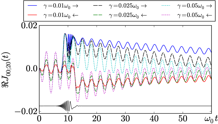
Figure 3: Time evolution of the propagating function elements associated with stationary coherences. $J_{00;20}(t)$ induced by the chirped pulse in Eq. (12) with $\omega_{\mathrm{D}}=\omega_{0}$ and $\hbar\omega_{0}/k_{\mathrm{B}}T=40$. Here $\omega_{0}t_{0}=10$, $\Omega_{\mathrm{L}}=10\omega_{0}$, $\Delta t\omega_{0}=4$ and $\sqrt{|S(\omega_{0})|}/\mathcal{E}_{0}=0.003415$ with $\chi=2.5$ [($\rightarrow$) continuous blue, dashed black and dotted cyan curves] and $\chi=-2.5$ [($\leftarrow$) continuous red, dashed green and dotted magenta curves] for various values of the coupling constant $\gamma$.

This being the case, the spectral phase information contained in the propagating functions element $J_{00;20}$ can now affect the dynamics of the expectation value in Eq. (3). Figure 3 shows $J_{00;20}$ as a function of time for $\chi=2.5$ (continuous blue, dashed black and dotted cyan curves) and $\chi=-2.5$ (continuous red, dashed green and dotted magenta curves) and for three different values of the coupling constant $\gamma=0.01\omega_{0}$, $\gamma=0.025\omega_{0}$ and $\gamma=0.05\omega_{0}$.

Remarkably, in Fig. 3, $J_{00;20}(t)$ shows a time dependence before the laser excitation occurs, resulting from the time dependence of the antisymmetric correlation function $A(t)$. This is a manifestation of an an incoherent flux at equilibrium between eigenstates. The detailed origin of this incoherent flux is well beyond the scope of this work and will be discussed elsewhere.

IV.3 Effect of Time-reversal-symmetry Breaking

The discussion above focused upon stationary features of non-unitary evolution that assist OPPC. Here we consider dynamical features (time-reversal-symmetry breaking) in non-unitary evolution that enhance OPPC. For this propose it suffices to study one of the propagating function elements. For example, the $J_{00;00}(t)$ element reads

$$\begin{split}J_{00;00}(t)=\sqrt{\frac{1}{q_{0}^{4}}\frac{2^{4}}{\det\mathsf{M}}}\frac{1}{N(t)}\exp\left(\frac{1}{2}\mathsf{E}^{\mathrm{T}}\mathsf{A}\mathsf{E}\right),\end{split}$$ (22)

Based on Eq. (21), it is clear that the propagating element $J_{00;00}(t)$ depends on the electric field phase in the long time regime for the open system case, thus allowing for the encoding of phase information.

Fig. 4 shows $J_{00;00}(t)$ using the same parameters as in Fig. 3.

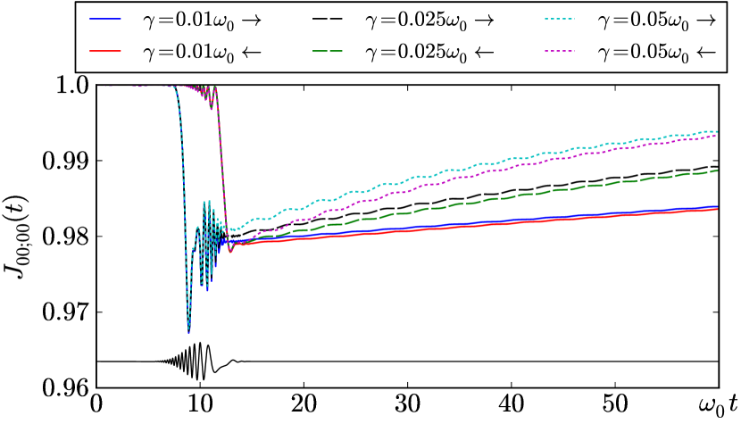
Figure 4: Time evolution of the propagating function elements associated to populations. $J_{00;00}(t)$ induced by the chirped pulse in Eq. (12). Parameter values as in Fig. 3.

For the unitary case [see Fig. 1], after the pulse is over there is no phase information in $J_{00;00}(t)$. However, for the non-unitary dynamics the effect of the phase persists in the long time regime, albeit diminished by the underlying incoherent thermal process. Further, the magnitude of the phase effect in $J_{00;00}(t)$, for short times after the pulse is over, is larger for the larger values of the coupling to the environment. However, in the long time regime, due to the equilibration, the phase information is lost.

IV.4 Control of Observables

Consider then, as an example, control over the population of the $n$-th system eigenstate, e.g., the population of the ground state, with $\hat{O}=|0\rangle\langle 0|$. Under unitary dynamics, and for an incoherent initial state, the time evolution of the ground state population is completely generated by the propagating function element $J_{00,00}(t)$ (see Fig. 1), and, as described above, no phase control is possible.

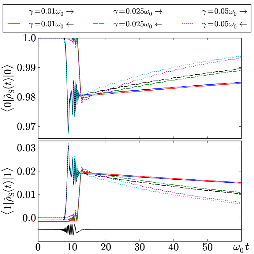
Figure 5: Influence of the coupling constant for the Ohmic spectral density. Time evolution of $\langle 0|\hat{\rho}(t)|0\rangle$ (upper panel) and $\langle 1|\hat{\rho}(t)|1\rangle$ (lower panel) induced by the chirped pulse in Eq. (12). Parameter values as in Fig. 3.

The situation is different in the presence of an environment. The upper panel of Fig. 5 shows the time evolution of the ground state population $\langle 0|\hat{\rho}_{\mathrm{S}}(t)|0\rangle$ using the same parameters as in Fig. 3. Here phase dependence of a quantity that commutes with the bare Hamiltonian $\hat{H}_{\mathrm{S}}$, is evident. Note that the full pulse effectively spans a time of $10\omega_{0}^{-1}$. Hence, although phase control must be lost over long times due to the environmental coupling, the control still survives over an extended time after the pulse is over, i.e., in a “non-equilibrated regime”.

The lower panel of Fig. 5 shows the time-evolution dynamics of the first excited state $\langle 1|\hat{\rho}(t)|1\rangle$. The characteristics of the phase dependence are similar to those for the ground state dynamics, the smaller phase amplitude and slower decay being the only noticeable differences. This arises from the very small initial population in $\langle 1|\hat{\rho}_{\mathrm{S}}(t)|1\rangle$ (0.000446 for $\gamma=0.01\omega_{0}$, 0.00113 for $\gamma=0.025\omega_{0}$ and 0.00223 for $\gamma=0.05\omega_{0}$) and the fact that for the times where the amplitude of the phase dependence is moderate, immediately after the pulse, the propagating elements $J_{11;\nu\mu}$ are small. In particular, the term responsible for the transfer of population from the ground state, $J_{11;00}$, behaves as $\sim\frac{1}{2}\mathsf{E}^{\mathrm{T}}\mathsf{A}\mathsf{E}\exp\left(\frac{1}{2}\mathsf{E}^{\mathrm{T}}\mathsf{A}\mathsf{E}\right)$ whereas $J_{00;00}$ behaves as $\sim\exp\left(\frac{1}{2}\mathsf{E}^{\mathrm{T}}\mathsf{A}\mathsf{E}\right)$ [see Eq. (22)].

In both panels of Fig. 5 one observes that, after the pulse is over, the state populations reach certain chirp-dependent values and then relax. Comparing the results in Fig. 5 with the time evolution of the $J_{00;00}$ element in Fig. 4, shows that the phase dependence, for this set of parameters, is primarily dictated by $J_{00;00}$, with no appreciable influence from the stationary coherence $\langle 0|\hat{\rho}_{\mathrm{S}}(0)|2\rangle$. This is a result of the small value of $J_{00;20}(t)\langle 0|\hat{\rho}_{\mathrm{S},\beta}|2\rangle$, which is the leading off-diagonal-contribution to the dynamics of $\langle 0|\hat{\rho}_{\mathrm{S}}(0)|0\rangle$. In particular, for $\gamma=0.01\omega_{0}$ we have that $\langle 0|\hat{\rho}_{\mathrm{S},\beta}|2\rangle=-0.00088$; while for $\gamma=0.025\omega_{0}$ and $\gamma=0.05\omega_{0}$, we have that $\langle 0|\hat{\rho}_{\mathrm{S},\beta}|2\rangle=-0.00219$ and $\langle 0|\hat{\rho}_{\mathrm{S},\beta}|2\rangle=-0.00435$, respectively. The off-diagonal element contribution may well be larger for other kinds of systems and couplings.

Given our goal of significant phase control, Fig. 2 suggests that we increase, e.g., the ratio $\gamma/\omega_{0}$. However, doing so would also induce faster decay rates, and the phase dependence would quickly vanish. Alternately, since the thermal energy at room temperature is $\sim 1/40$ eV and energy of the optical transitions are between 1.6 to 3.4 eV, increasing the ratio $\hbar\omega_{0}/k_{\mathrm{B}}T$ could be a more promising alternative to enhance control. However, as seen from Fig. 2, for $\hbar\omega_{0}/k_{\mathrm{B}}T>10$, $\langle 0|\hat{\rho}_{\beta}|2\rangle$ becomes basically temperature-independent. Thus environmentally assisted phase control has the fundamental challenge that the terms that assist control also induce, simultaneously, equilibration with the bath.

IV.5 Influence of the Non-Markovian Character of the Dynamics

In general, open quantum systems undergo non-Markovian provide that the spectrum of the thermal fluctuations is not flat (coloured noiseHänggi and Jung (2007)). Formally, the Markovian regime is reached when the spectral density has a linear monotonic behaviour and thermal energy $k_{\mathrm{B}}T$ is the larger energy scale of the system. For the Ohmic spectral density in Eq. (17), increasing $\omega_{\mathrm{D}}$ is known to bring the system closer to the Markovian limit. To examine the non-Markovian effects we show, in Fig. 6, the time evolution of the ground state and first excited state, generated by the laser pulse for different values of the cutoff frequency $\omega_{\mathrm{D}}$. The amplitude of the phase effect, for short times after the pulse is over, is seen to be larger for the Markovian cases ($\omega_{\mathrm{D}}=10\omega_{0}$ and $\omega_{\mathrm{D}}=100\omega_{0}$) than for the non-Markovian case ($\omega_{\mathrm{D}}=\omega_{0}$). This reflects the stronger effective system-bath coupling in the Markovian case Pachón, Triana, and Brumer (2013). As a consequence, the time reversibility of the unitary dynamics is lost more effectively in the non-Markovian case. However, in the long time regime the non-Markovian dynamics, due to its weaker effective coupling to the bath, has a larger phase-effect, albeit the overall phase control is very small.

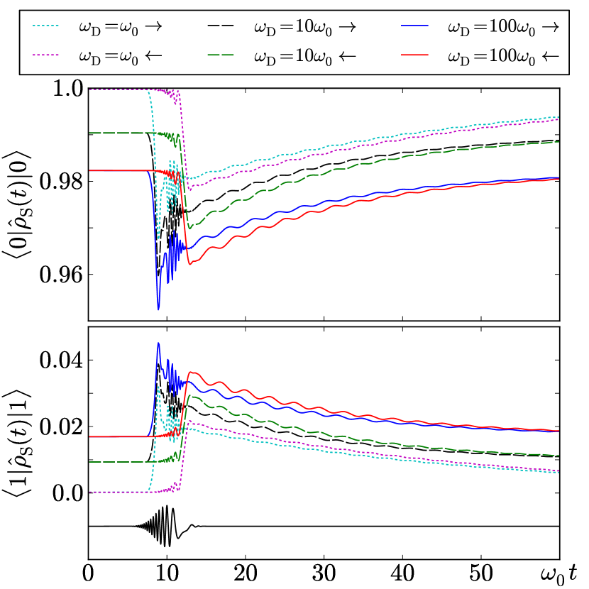
Figure 6: Influence of the non-Markovian character of the dynamics. Time evolution of $\langle 0|\hat{\rho}_{\mathrm{S}}(t)|0\rangle$ (upper panel) and $\langle 1|\hat{\rho}_{\mathrm{S}}(t)|1\rangle$ (lower panel) with $\gamma=0.05\omega_{0}$ and $\hbar\omega_{0}/k_{\mathrm{B}}T=40$ for different values of the cutoff frequency $\omega_{\mathrm{D}}$. The value of the laser parameters are as in Fig. 3.

IV.6 Effect of the a Different Spectral Density

Although the main lines of the above discussion are general and intuitive, the numerical results above pertain to the Ohmic spectral density [17]. Motivated by our recent observationPachón and Brumer (2013c) that the effect of the vibrations and the solvent– in systems such as dye molecules, amino acid proteins and some photochemical systems (e.g., rhodopsin and green fluorescence proteins)– could be effectively described by a sub-Ohmic spectral density; we consider this alternate spectral density below. Note that sub-Ohmic spectral densities are characterized by slow decay rates, even in the strong coupling regimePachón and Brumer (2013c). Hence, this spectral density may well be of some interest in terms of phase-control, where it may result in a prolonged phase-control effect.

The sub-Ohmic spectral density with exponential decay is given by

$$J_{\mathrm{sOhm}}(\omega) =m\gamma\omega_{\mathrm{ph}}^{1-s}\omega^{s}\,\exp\left(-\omega/\omega_{\mathrm{D}}\right),$$ (23)

with $0<s<1$, and $\omega_{\mathrm{ph}}$ is an auxiliary phononic scale frequency. For this case the relevant coupling constant is $\gamma\omega_{\mathrm{ph}}^{1-s}$ and the spectral density generates the dissipative kernel $\gamma(s)=\frac{4}{\pi}\left(1+t^{2}\omega_{\mathrm{D}}^{2}\right)^{-s/2}\omega_{\mathrm{ph}}^{1-s}\Gamma(s)\cos\left[s\arctan(\omega_{\mathrm{D}}t)\right]$. In the limit where $\omega_{\mathrm{D}}\rightarrow\infty$, $\gamma(t)\rightarrow\frac{4}{\pi}t^{-s}\omega_{\mathrm{ph}}^{1-s}\Gamma(s)\cos\left(\frac{\pi}{2}s\right)$ which, by contrast to the Ohmic case, also leads to non-Markovian effects. In the short time regime, $\omega_{\mathrm{D}}t\ll 1$, $\gamma(t)/\gamma(0)\sim 1-\frac{1}{2}s(1+s)(\omega_{\mathrm{D}}t)^{2}$, which resembles the functional form of a Gaussian decay at short times. In the long time regime, $\omega_{\mathrm{D}}t\gg 1$, $\gamma(t)/\gamma(0)\sim\cos(\frac{\pi}{2}s)(\omega_{\mathrm{D}}t)^{-s}$, so that the long time decay is only algebraic, $1/t^{s}$.

Fig. 7 shows the sub-Ohmic analog of the Ohmic calculation in the upper panel in Fig. 2, where values of the stationary off-diagonal element $\langle 0|\hat{\rho}_{\mathrm{S},\beta}|2\rangle$, larger than in the Ohmic case, are seen.

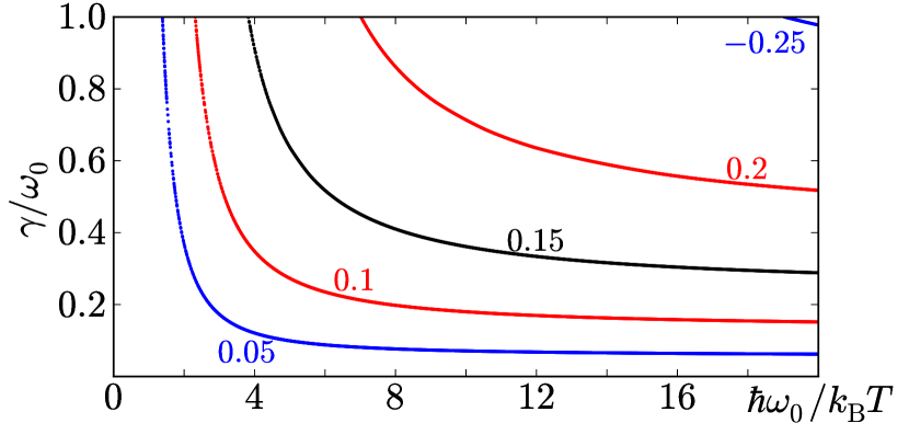
Figure 7: Stationary coherence generated by the sub-Ohmic spectral density. Contours of constant matrix element $\langle 0|\hat{\rho}_{\mathrm{S},\beta}|2\rangle$ as a function of $\gamma$ and $T$ for fixed $\omega_{\mathrm{ph}}=\omega_{0}$, $\omega_{\mathrm{D}}=\omega_{0}$ and $s=0.1$.

Figure 8 shows the time evolution of the ground and first excited states, where the system-bath interaction is described by a sub-Ohmic spectral density [23] and where the parameters are the same as those in Fig. 5 The new feature seen here is the persistence of population oscillations in the ground state which is also present, although to lesser extent, in the first excited state. This observation is consistent with the recent finding that sub-Ohmic spectral densities are able to maintain coherent oscillations for longer times in the spin-boson modelKast and Ankerhold (2013).

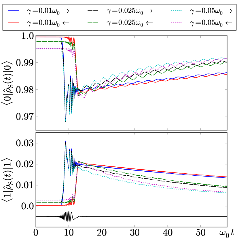
Figure 8: Influence of the coupling constant for the sub-Ohmic spectral density. Time evolution of $\langle 0|\hat{\rho}_{\mathrm{S}}|0\rangle$ induced by the chirped pulse in Eq. (12). with and $\hbar\omega_{0}/k_{\mathrm{B}}T=40$, $\omega_{\mathrm{ph}}=\omega_{0}$, $\omega_{\mathrm{D}}=\omega_{0}$ and $s=0.1$. The value of the laser parameters are as in Fig. 3.

One further feature occurs at short times where, the phase amplitude is slightly larger in the sub-Ohmic case than in the Ohmic case. However, due to the Gaussian-like decay discussed above, this larger phase dependence decays faster here than in the Ohmic case (where for short times, the decay is exponential). However, this fast relaxation is compensated by the long-time algebraic decay (see above), so that some phase-information persists in the system at long times.

V Discussion

In the model system examined here, phase controllability was successfully demonstrated, primarily mediated by the breaking of time-reversal symmetry, which is a completely incoherent process. Although we could not observe any significant effect of the off-diagonal elements (stationary coherences) during the control phase, the fact that it can reach large values (see Fig. 7) implies that these terms must be included in any treatment of phase control and may well be influential in other model systems.

We note that there is a fundamental difference in the nature of control mechanisms arising via the time-reversal symmetry and the stationary coherences. Specifically, the first is an effect that can arise in either classical or quantum mechanics. Indeed, proving that the origin of such experimentally observed control is quantum, e.g., via a Bell inequalityScholak and Brumer (2013), is far from a trivial task. By contrast, the off-diagonal elements vanish in classical mechanicsCampisi, Talkner, and Hänggi (2009). Hence, they are quantum in nature, arising from the entanglement between the system and the bath. Although in our case the contribution of the off-diagonal elements is of second order in the effective coupling to the bathPachón, Triana, and Brumer (2013), and therefore is expected to be small, any successful observation of the role of the off-diagonal elements in OPPC will signal a pure quantum effect.

Indeed, it should be noted that, to date, there is no experimental demonstration of environmentally assisted one photon phase control. The originalProkhorenko et al. (2006); Joffre (2007); Prokhorenko et al. (2007) or related experimentsProkhorenko, Halpin, and Miller (2011) in which this mechanism was invoked, as well as the related computational workArango and Brumer (2013), showed phase control of cis-trans isomerization. However, the property “cis-or-trans” consists of a projection onto a spatial domain, and hence is an operator that does not commute with the system Hamiltonian. As such, one knowsSpanner, Arango, and Brumer (2010); Pachón, Yu, and Brumer (2013) that phase control is possible even in the absence of an environment. Rather, the environment in case of isomerization serves to relax the system into one of the two isomers. The insights afforded by the analysis in this paper should serve to motivate new studies to experimentally demonstrate one photon phase control.

Appendix A Evolution of the density operator

The matrix $\mathsf{A}$ contains the information about the open system evolution and is defined as

$$\mathsf{A} =\frac{1}{q_{0}^{6}\det\mathsf{M}}\left(\begin{array}[]{cc}1+\mathsf{A}_{11}&\mathsf{A}_{12}\\ \mathsf{A}_{12}&1+\mathsf{A}_{22}\end{array}\right),$$ (26)

being

$$\begin{split}\mathsf{A}_{11}&=\frac{m^{2}}{\hbar^{2}\omega_{0}^{2}\Lambda^{2}}\left(1-2\Lambda\omega_{0}\right)\left[\frac{\dot{G}_{+}(t)}{G_{+}(t)}S(t)-\dot{S}(t)\right]^{2}+\left(1+2\Lambda\omega_{0}\right)\frac{\dot{G}_{+}^{2}(t)}{\omega_{0}^{2}G_{+}^{2}(t)}+\frac{2\Omega}{\omega_{0}},\end{split}$$ (27)

$$\begin{split}\mathsf{A}_{12}&=\frac{m^{3}}{\hbar^{3}\omega_{0}\Lambda^{2}}\frac{S(t)}{G_{+}(t)}\left[\frac{\dot{G}_{+}(t)}{G_{+}(t)}S(t)-\dot{S}(t)\right]\left[\frac{S(t)}{G_{+}(t)}-2\Lambda\omega_{0}\right],\end{split}$$ (28)

$$\begin{split}\mathsf{A}_{22}&=\frac{m^{2}}{\hbar^{2}\omega_{0}^{2}\Lambda^{2}}\left(1-2\Lambda\omega_{0}\right)\frac{S^{2}(t)}{G^{2}_{+}(t)}+\left(1+2\Lambda\omega_{0}\right)\frac{1}{\omega_{0}^{2}G_{+}^{2}(t)}-\frac{2\Omega}{\omega_{0}}.\end{split}$$ (29)

$\Lambda$ is related to the second moment in equilibrium of the $\hat{q}$ by means of $\langle\hat{q}^{2}\rangle=\hbar\Lambda/m$ while $\Omega$ through $\langle\hat{p}^{2}\rangle=\hbar m\Omega$ Grabert, Schramm, and Ingold (1988). $S(t)$ denotes the symmetric position autocorrelation function, $S(t)=\frac{1}{2}\langle\hat{q}(t)\hat{q}+\hat{q}\hat{q}(t)\rangle$. In the limit $\omega_{\mathrm{D}}\rightarrow\infty$, it is given by

$$\begin{split}S(t)&=\frac{\hbar}{4m\omega_{\mathrm{d}}}[\exp(-\lambda_{2}t)\coth(\textrm{\textonehalf}\mathrm{i}\hbar\beta\lambda_{2})-\exp(-\lambda_{1}t)\coth(\textrm{\textonehalf}\mathrm{i}\hbar\beta\lambda_{1})]-\Gamma(t),\end{split}$$ (30)

$$\Gamma(t) =\frac{\gamma}{m\beta}\sum_{n=-\infty}^{\infty}\frac{|\nu_{n}|\exp(-|\nu_{n}|t)}{(\omega_{0}^{2}+\nu_{n}^{2})^{2}-\gamma^{2}\nu_{n}^{2}},$$ (31)

being $\nu_{n}=2\pi n/\hbar\beta$ the Matsubara frequencies (cf. Ref. 34; 32).

The matrix $\mathsf{M}$ is given by

$$\mathsf{M}(t)=\frac{m}{\hbar}\left(\begin{array}[]{cccc}R^{--}(t)&-\mathrm{i}\frac{\dot{G}_{+}(t)}{G_{+}(t)}&-C_{2}^{-}(t)+R^{+-}(t)&\mathrm{i}\frac{1}{G_{-}(t)}-\mathrm{i}C_{1}^{-}(t)\\ -\mathrm{i}\frac{\dot{G}_{+}(t)}{G_{+}(t)}&0&\mathrm{i}\frac{1}{G_{+}(t)}&0\\ -C_{2}^{-}(t)+R^{+-}(t)&\mathrm{i}\frac{1}{G_{+}(t)}&-2C_{2}^{+}(t)+R^{++}(t)&-\mathrm{i}\frac{\dot{G}_{+}(t)}{G_{+}(t)}-\mathrm{i}C_{1}^{+}(t)\\ \mathrm{i}\frac{1}{G_{-}(t)}-\mathrm{i}C_{1}^{-}(t)&0&-\mathrm{i}\frac{\dot{G}_{+}(t)}{G_{+}(t)}-\mathrm{i}C_{1}^{+}(t)&0\end{array}\right),$$ (32)

being

$$C_{j}^{+}(t)=\int\limits_{0}^{t}\mathrm{d}s C_{j}(s)\frac{G_{+}(t-s)}{G_{+}(t)},\qquad C_{j}^{-}(t)=\int\limits_{0}^{t}\mathrm{d}sC_{j}(s)\frac{G_{-}(s)}{G_{-}(t)},$$ (33)

$$R^{+-}(t) =\int_{0}^{t}\mathrm{d}s\int_{0}^{t}\mathrm{d}uR(s,u)\frac{G_{+}(t-s)}{G_{+}(t)}\frac{G_{-}(u)}{G_{-}(t)},$$ (34)

with $R^{++}(t)$ and $R^{--}(t)$ defined accordingly.