Higgs Boson Phenomenology in a Simple Model with Vector Resonances

Abstract

In this paper we consider a simple scenario where the Higgs boson and two vector resonances are supposed to arise from a new strong interacting sector. We use the ATLAS measurements of the dijet spectrum to set limits on the masses of the resonances. Additionally we compute the Higgs boson decay to two photons and found, when compare to the Standard Model prediction, a small excess which is compatible with ATLAS measurements. Finally we make prediction for Higgs-strahlung processes for the LHC running at 14 TeV.

1 Introduction

The 125 GeV Higgs boson recently discovered at the LHC [1, 2] seems to behave in a very standard way. No important deviation from the Standard Model (SM) predictions has been found except for Mass 2013a small discrepancy in its decay to two photons which still survives in ATLAS measurements. As a result, stringent constraints have been put on an eventual New Physics at the TeV scale. The Minimal Supersymmetric Standard Model (MSSM), for instance, seems to suffer from serious tensions trying to accommodate simultaneously such a large mass for the lighter Higgs boson and the current non-observability of any “super-partner” at the TeV scale . Indeed, the current exploration of supersymmetric alternatives to the Standard Model, in general, seems to need a structure that goes beyond the minimal possibility[3]. On the other hand, the LHC has evidently ruled out a complete family of Dynamical Electroweak Symmetry Breaking (DEWSB) models which predicted a Higgsless low energy spectrum. Nevertheless, there are some classes of DEWSB models which predict a light composite Higgs boson and still offer a viable explanation for the stability of the Electroweak scale. For instance, Walking Technicolor (WTC)[4, 5, 6] and models where the Higgs is a pseudo-Goldstone boson are notable examples of such kind of models with a light scalar in the spectrum[7, 8, 9].

In this paper, we consider a scenario where a new strong interacting sector originates the Fermi scale and manifests itself by means of a composite scalar boson (which we identify with the 125 GeV Higgs boson) and vector resonances. In order to make this scenario concrete, we use a simple phenomenological model proposed by one of us some year ago[10]. In this model, two kind of vector resonances are included: a triplet of $SU(2)_{L}$ (which can be thought as a “techni-rho” and then we denote it by $\rho_{\mu}$) and a singlet of $SU(2)_{L}$ (which can be thought as a “techni-omega” and then we denote it by $\omega_{\mu}$). It is assumed that these new states interact with the particles of the SM by their mixing with the standard gauge bosons $W_{\mu}^{a}$ and $B_{\mu}$ in analogy to the well known Vector Meson Dominance (VMD) mechanism in Hadron Physics. Originally, this setup was used to point out that in a Composite Higgs framework an enhancement of the associate production of a Higgs and a gauge boson could be expected. This result was later confirmed by other authors in the context of Minimal Walking Technicolor (MWTC)[11]. It has also been shown that MWTC also predicts a deviation of the Higgs to two photons decay ratio, compared with the SM.

In this work, we use the simple framework described above and data from the ATLAS Collaboration to set limits on the masses of the vector resonances. Additionally, we make some predictions for the next run of the LHC. Finally, based on our results, we comment on some characteristics we think must be respected by DEWSB scenarios.

The paper is organized in the following way. In section 2 we describe the theoretical construction. Section 3 is devoted to set limits on the mass of the resonances based on dijet measurements. In section 4 we evaluate the consistency of the model with the current measurement of $\Gamma(h\rightarrow\gamma\gamma)$. In section 5 we compute Higg-strahlung processes for the LHC at $\sqrt{s}=14$ TeV. Finally, in section 6 we comment our results and state our conclusions.

2 The Model

The model studied in this work was already proposed elsewhere by one of us[10]. Nevertheless, in regard of the completeness, we dedicate this section to a presentation of the main characteristics of our theoretical construction.

2.1 Gauge Sector

As explained above, our model contains two new vector fields which are supposed to be the manifestation of an underlying strong sector. We assume that these resonances interact with the standard sector through their mixing with the electroweak gauge bosons, following the VMD idea. In a more modern but equivalent language, the model can be formulated based on the “moose” diagram shown in figure 1.

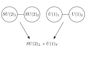
Figure 1: Gauge structure of the model. Our construction may be thought as coming from a moose diagram like the one shown here. The initial gauge symmetry $SU(2)_{1}\times SU(2)_{2}\times U(1)_{1}\times U(1)_{2}$ is broken down (by a non-linear sigma sector, for example) to $SU(2)_{L}\times U(1)_{Y}$ and our effective Lagrangian (1) is obtained.

The resulting low energy Lagrangian (assuming that the Abelian and non-Abelian parts break at the same scale) can be written as:

$${\cal L} = -\frac{1}{2}\mathrm{Tr\left\{W_{\mu\nu}W^{\mu\nu}\right\}}-\frac{1}{2}\mathrm{Tr}\left\{\tilde{\rho}_{\mu\nu}\tilde{\rho}^{\mu\nu}\right\}$$ (1)

$$-\frac{1}{4}B_{\mu\nu}B^{\mu\nu}-\frac{1}{4}\tilde{\omega}_{\mu\nu}\tilde{\omega}^{\mu\nu}$$

$$+M^{2}\mathrm{Tr}\left\{\left(\frac{g}{g_{2}}W_{\mu}-\tilde{\rho}_{\mu}\right)^{2}\right\}+\frac{M^{2}}{2}\left(\frac{g^{\prime}}{g{}_{2}}B_{\mu}-\tilde{\omega}_{\mu}\right)^{2}.$$

where $W_{\mu}$ and $B_{\mu}$ are the fields associated to the sites labeled by “1” while $\tilde{\rho}_{\mu}$ and $\tilde{\omega}_{\mu}$ are associated to the sites labeled by “2” and assumed to be strongly coupled. As usual, $W_{\mu\nu}$ , $\tilde{\rho}_{\mu\nu}$, $B_{\mu\nu}$ and $\tilde{\omega}_{\mu\nu}$ are (in term of components)

$$W_{\mu\nu}^{a} = \partial_{\mu}W_{\nu}^{a}-\partial_{\nu}W_{\mu}^{a}+g\epsilon^{abc}W_{\mu}^{b}W_{\nu}^{c},$$ (2)

$$\tilde{\rho}_{\mu\nu}^{a} = \partial_{\mu}\tilde{\rho}_{\nu}^{a}-\partial_{\nu}\tilde{\rho}_{\mu}^{a}+g_{2}\epsilon^{abc}\tilde{\rho}_{\mu}^{b}\tilde{\rho}_{\nu}^{c},$$ (3)

$$B_{\mu\nu} = \partial_{\mu}B_{\nu}-\partial_{\nu}B_{\mu},$$ (4)

$$\tilde{\omega}_{\mu\nu} = \partial_{\mu}\tilde{\omega}_{\nu}-\partial_{\nu}\tilde{\omega}_{\mu}.$$ (5)

By construction, Lagrangian (1) is invariant under $SU(2)_{\mbox{L}}\times U(1)_{\mbox{Y}}$. The symmetry breaking to $U(1)_{\mbox{em}}$ will be described by means of the vacuum expectation value of a scalar field, as in the Standard Model. In other words, we will use an effective gauged linear sigma model as a phenomenological description of the electroweak symmetry breaking.

2.2 Fermion Sector

As usual, fermions are coupled to the gauge fields through covariant derivatives:

$${\cal L}=\overline{\psi_{L}}i\gamma^{\mu}D_{\mu}\psi_{L}+\overline{\psi_{R}}i\gamma^{\mu}\tilde{D}_{\mu}\psi_{R},$$ (6)

with

$$D_{\mu} = \partial_{\mu}+i\tau^{a}g(1-x_{1})W_{\mu}^{a}+i\tau^{a}g_{2}x_{1}\tilde{\rho}_{\mu}^{a}$$ (7)

$$+i\frac{Y}{2}g^{\prime}(1-x_{2})B_{\mu}+i\frac{Y}{2}g^{\prime}_{2}x_{2}\tilde{\omega}_{\mu}$$

and

$$\tilde{D}_{\mu}=\partial_{\mu}+i\frac{Y}{2}g^{\prime}(1-x_{3})B_{\mu}+i\frac{Y}{2}g^{\prime}_{2}x_{3}\tilde{\omega}_{\mu}.$$ (8)

The parameters $x_{i}$ ($i=1,2,3$) play the role of fermion delocalization [12] and in our case govern the direct coupling to the new vector bosons. In the context of the BESS model [13, 14], which shares with our model a similar structure in the spin-1 sector, it has been shown that a direct interaction of order $2(g/g_{2})^{2}$ is necessary in order to reconcile the model with the precision electroweak parameters $S$, $T$ and $U$. Hence, we adopt this result and impose $x_{i}=2(g/g_{2})^{2}$ for $i=1,2,3$.

2.3 Higgs Sector and EWSB

In our effective model, the Higgs sector is assumed to be the same as in the Standard Model except by the possibility of including a direct coupling, between the Higgs doublet and the vector resonances, depending on how the Higgs boson is localized. In this way, the Lagrangian for the Higgs sector can be written as:

$${\cal L}=\left(D^{\mu}\Phi\right)^{\dagger}\left(D_{\mu}\Phi\right)-V\left(\Phi\right),$$ (9)

where, as usual

$$V\left(\Phi\right)=-\mu^{2}\Phi^{\dagger}\Phi+\lambda\left(\Phi^{\dagger}\Phi\right)^{2},$$ (10)

and

$$D_{\mu} = \partial_{\mu}+i\tau^{a}g(1-f_{1})W_{\mu}^{a}+i\tau^{a}g_{2}f_{1}\tilde{\rho}_{\mu}^{a}$$ (11)

$$+i\frac{Y}{2}g^{\prime}(1-f_{2})B_{\mu}+i\frac{Y}{2}g^{\prime}_{2}f_{2}\tilde{\omega}_{\mu}.$$

For simplicity, we chose to completely localize the Higgs fields in the weakly coupled sites imposing $f_{i}=0$ for $i=1,2$. The consequences of these choice will be discussed later.

Once the electroweak symmetry is broken, two non-diagonal mass matrices are generated: one for the neutral vector bosons and another for the charged one

$${\cal M_{\mbox{neutral}}}=\frac{v^{2}}{4}\left[\begin{array}[]{cccc}(1+\alpha^{2})g^{2}&-\alpha^{2}gg_{2}&-gg^{\prime}&0\\ -\alpha^{2}gg_{2}&\alpha^{2}g_{2}^{2}&0&0\\ -gg^{\prime}&0&(1+\alpha^{2})g{}^{\prime 2}&-\alpha^{2}g^{\prime}g_{2}\\ 0&0&-\alpha^{2}g^{\prime}g_{2}&\alpha^{2}g{}^{\prime 2}\end{array}\right],$$ (12)

$${\cal M_{\mbox{charged}}}=\frac{v^{2}}{4}\left[\begin{array}[]{cc}(1+\alpha^{2})g^{2}&-\alpha^{2}gg_{2}\\ -\alpha^{2}gg_{2}&\alpha^{2}g_{2}^{2}\end{array}\right],$$ (13)

where

$$\alpha^{2}=\frac{4M^{2}}{v^{2}g_{2}^{2}}.$$ (14)

Notice that $\alpha v$ may be thought as the scale where the mass of the rho and omega resonances is generated. It is natural to identify this scale with the natural scale of the strong sector which in our case is $\Lambda=4\pi v$. Consequently, we assume that the natural value of $\alpha$ is $\alpha=4\pi$. Notice that $\Lambda$ is also a natural upper limit for the value of the mass of the resonances. Additionally, we have assume that the new vector resonance are degenerated in mass.

The mass matrices can be diagonalized and the eigenvectors, in the limit $g/g_{2}\ll 1$ and keeping terms up to order $g/g_{2}$, can be written as:

$$A = \frac{g^{\prime}}{\sqrt{g^{2}+g^{\prime 2}}}W^{3}+\frac{g}{\sqrt{g^{2}+g^{\prime 2}}}B+\frac{gg^{\prime}}{g_{2}\sqrt{g^{2}+g^{\prime 2}}}\tilde{\rho}^{3}+\frac{gg^{\prime}}{g_{2}\sqrt{g^{2}+g^{\prime 2}}}\tilde{\omega},$$

$$Z = \frac{g}{\sqrt{g^{2}+g^{\prime 2}}}W^{3}-\frac{g^{\prime}}{\sqrt{g^{2}+g^{\prime 2}}}B+\frac{g^{2}}{g_{2}\sqrt{g^{2}+g^{\prime 2}}}\tilde{\rho}^{3}-\frac{g^{\prime 2}}{g_{2}\sqrt{g^{2}+g^{\prime 2}}}\tilde{\omega},$$

$$\rho^{0} = -\frac{g}{g_{2}}W^{3}+\tilde{\rho}^{3},$$ (15)

$$\omega = -\frac{g^{\prime}}{g_{2}}B+\tilde{\omega},$$

$$W^{\pm} = \tilde{W}^{\pm}+\frac{g}{g_{2}}\tilde{\rho}^{\pm},$$

$$\rho^{\pm} = \tilde{\rho}^{\pm}-\frac{g}{g_{2}}\tilde{W}^{\pm},$$

where

$$\tilde{W}^{\pm}=\frac{1}{\sqrt{2}}\left(W^{1}\mp iW^{2}\right)$$ (16)

and

$$\tilde{\rho}^{\pm}=\frac{1}{\sqrt{2}}\left(\tilde{\rho}^{1}\mp i\tilde{\rho}^{2}\right).$$ (17)

We used LanHEP [15] to implement this model into the CalcHEP package[16].

3 Limits from the Dijet Spectrum

As a first step, we proceed to obtain limits for the mass of the resonances using the dijet spectrum measured by ATLAS[17]. For this purpose, we generated events for the $pp\rightarrow jj$ process at $\sqrt{s}=8$ TeV using CalcHEP, considering only the contribution of the new vector resonances. In order to compare with ATLAS data we imposed the following kinematic cuts:

$$\frac{1}{2}\left|y_{1}-y_{2}\right| < 0.6,$$ (18)

$$\left|y_{1,2}\right| < 2.8,$$ (19)

$$M_{jj} > 1000\>\mathrm{GeV,}$$ (20)

$$p_{T1,2} > 150\>\mathrm{GeV,}$$ (21)

where $y$ refers to the jet rapidity, $p_{T}$ is its transverse momentum and $M_{jj}$ is the invariant mass of the two jets. The main contribution to this process comes from the production of the rho and omega in the s-channel through quark–anti-quark annihilation. Unfortunately, due to PDF effects, it is unlikely to produce anti-quarks with large momentum at the LHC and a considerable fraction of the events are produced in the low $M_{jj}$ region. Of course, such events are hidden under the background. In consequence we select only the resonant part of our events in order to compare it with the experimental upper limits. For doing that, and after imposing the cuts, we fit the events around the resonant peak with a Breit-Wigner function and a second degree polynomial, describing the non-resonant “background”, and define our resonant events as the integral of the Breit-Wigner function. Now we are prepared to compare with experimental data. Our results are shown in figure 2. There, the ATLAS upper limits for invisible resonances are compared to our predicted cross section for dijet production considering only the contribution of the new vector fields and the appropriate kinematic cuts. Everything above the experimental curve is excluded. In our case, that means that our model is consistent with the ATLAS dijet measurements provided that the mass of the vector resonances satisfies the constrain $M\gtrsim 2200$ GeV.

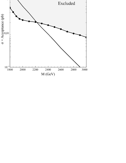
Figure 2: Resonant cross sections (continuous line) compared to ATLAS upper limits to narrow resonances decaying into dijet (dots with continuous line), as a function of the resonance mass. The colored region is excluded.

4 $h\rightarrow\gamma\gamma$

A relevant observable in Higgs phenomenology is its decay rate into two photons. This is the only measured quantity that presents a sensible deviation from the SM, at least in results reported by ATLAS. Since it is a loop effect, we expect that this observable is sensible to the existence of New Physics. With this motivation in mind, we computed the $\Gamma(h\rightarrow\gamma\gamma)$ in our model at one loop level. Non-standard contributions arise through the presence of the $\rho_{\mu}^{\pm}$ fields. The new diagrams are formally the same that those generated by the $W_{\mu}^{\pm}$ bosons except, obviously, by the different values of the coupling constants (which in case of the $h\rho^{+}\rho^{-}$ is suppressed by a factor $(g/g_{2})^{2}$ with respect to $hW^{+}W^{-}$) and the vector boson masses. The result is shown in figure 3 where we have plotted the ratio

$$R_{\gamma}=\frac{\Gamma(h\rightarrow\gamma\gamma)_{Model}}{\Gamma(h\rightarrow\gamma\gamma)_{SM}}$$ (22)

as a function of the rho mass. We see that in the allowed range of masses, $R_{\gamma}$ varies from 1.25 to 1.50. This result has to be compared with the experimental values[18, 19]:

$$R_{\gamma}=\begin{cases}1.6\pm 0.3&\mathrm{ATLAS}\\ 0.77\pm 0.27&\mathrm{CMS}.\end{cases}$$ (23)

Notice that our results agree with the experimental values at $1\sigma$ level in the case of ATLAS and at $2.5\sigma$ level in the case of CMS

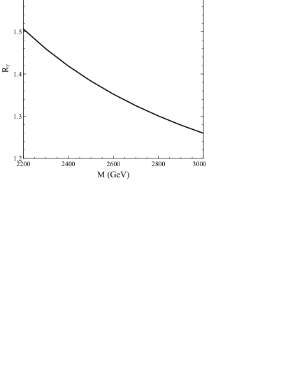
Figure 3: Predicted values of $R_{\gamma}=\Gamma(h\rightarrow\gamma\gamma)_{Model}/\Gamma(h\rightarrow\gamma\gamma)_{SM}$

5 Higgs-strahlung

As explained above, the model studied in this paper was proposed by one of us some years ago. It was shown that for resonance masses that were reasonable at that time, the model presented a significant enhancement of associated production of a Higgs boson and a gauge boson. This result was confirmed later in the framework of the MWTC. Given this context, it is interesting to evaluate whether this channel remains robust after considering the limits imposed by current experimental data. Consequently, we used CalcHEP to compute the cross sections for the processes $pp\rightarrow Zh$ and $pp\rightarrow W^{+}h$ at $\sqrt{s}=14$ TeV due only to the contributions of the new spin-1 states and we compare it to the SM prediction. The result is shown in figure 4.

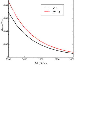
Figure 4: Predicted cross sections for the processes $pp\rightarrow Zh$ (continuous line) and $pp\rightarrow W^{+}h$ (dashed line) at $\sqrt{s}=14$ TeV due only to the contributions of the new spin-1 states compared to the SM prediction

Unfortunately, our results show a very small enhancement in the cross section: less than $10\%$ in the available mass range, which is unlikely to be testable at the LHC.

6 Summary and Conclusions

In this work we have reconsidered a simple model which contains two new spin-1 states, supposed to be composite together with the Higgs boson, pointing out to a strong dynamical origin of the Electroweak scale. We used dijet data from ATLAS to set limits on the mass of the new states. We found that current data allows masses in the range $2.2\>\mathrm{TeV}\lesssim M\lesssim 4\pi v\approx 3.1$ TeV .

Then, we computed $\Gamma(h\rightarrow\gamma\gamma)$ and compared with the SM prediction. We found that our result is compatible with recent measurements at the LHC. In this sense we can say that this simple model has passed the experimental test. This success is related to the fact that in our model the Higgs boson is weakly coupled to the new spin-1 states. This is a consequence of choosing $f_{1}=f_{2}=0$ in equation (11). The original motivation for this choice was to simplify the model and make sure we could faithfully reproduce the phenomenology of the $W^{\pm}$ and $Z$ bosons. Nevertheless, we see the agreement with the measured value of $R_{\gamma}$ as an a posteriori justification.

Unfortunately, on the other hand, the proposed enhancement in the Higgs-strahlung channels has not survived as an important signal of the model at the LHC.

Ackowledgements

ARZ has received financial support from Fondecyt grant nº 1120346. O.C-F. was supported by Fondecyt grant No. 11000287 and Basal Project FB0821. CC, GM, FR and JZ received support from Conicyt National Ph.D. Fellowship Program.

References

- [1] G. Aad et al. [ATLAS Collaboration], “Observation of1 a new particle in the search for the Standard Model Higgs boson with the ATLAS detector at the LHC,” Phys. Lett. B 716 (2012) 1 [arXiv:1207.7214 [hep-ex]].
- [2] S. Chatrchyan et al. [CMS Collaboration], “Observation of a new boson at a mass of 125 GeV with the CMS experiment at the LHC,” Phys. Lett. B 716 (2012) 30 [arXiv:1207.7235 [hep-ex]].
- [3] E. Hardy, “Is Natural SUSY Natural?”, arXiv:1306.1534 [hep-ph].
- [4] R. Foadi, M. T. Frandsen, T. A. Ryttov and F. Sannino, “Minimal Walking Technicolor: Set Up for Collider Physics,” Phys. Rev. D76, 055005 (2007) [arXiv:0706.1696 [hep-ph]].
- [5] T. A. Ryttov and F. Sannino, “Ultra Minimal Technicolor and its Dark Matter TIMP,” Phys. Rev. D78, 115010 (2008) [arXiv:0809.0713 [hep-ph]].
- [6] For a recent review of modern DEWSB models see: F. Sannino, “Conformal Dynamics for TeV Physics and Cosmology,” Acta Phys. Polon. B40 (2009) 3533 [arXiv:0911.0931 [hep-ph]].
- [7] N. Arkani-Hamed et al, JHEP 0208 (2002) 021, hep-ph/0206020; N. Arkani-Hamed, A. Cohen, E. Katz, and A. Nelson, JHEP 0207 (2002) 034, hep-ph/0206021; M. Schmaltz and D. Tucker-Smith, Ann.Rev.Nucl.Part.Sci. 55 (2005) 229, hep-ph/0502182; M. Perelstein, Prog.Part.Nucl.Phys. 58 (2007) 247, hep-ph/0512128; M. Perelstein, M. E. Peskin, and A. Pierce, Phys.Rev. D69 (2004) 075002, hep-ph/0310039.
- [8] D. B. Kaplan and H. Georgi, Phys. Lett. B 136 (1984) 183; S. Dimopoulos and J. Preskill, Nucl. Phys. B 199, 206 (1982); T. Banks, Nucl. Phys. B 243, 125 (1984); D. B. Kaplan, H. Georgi and S. Dimopoulos, Phys. Lett. B 136, 187 (1984); H. Georgi, D. B. Kaplan and P. Galison, Phys. Lett. B 143, 152 (1984); H. Georgi and D. B. Kaplan, Phys. Lett. B 145, 216 (1984).; M. J. Dugan, H. Georgi and D. B. Kaplan, Nucl. Phys. B 254, 299 (1985).
- [9] G. F. Giudice, C. Grojean, A. Pomarol and R. Rattazzi, JHEP 0706, 045 (2007), [hep- ph/0703164]; C. Csaki, A. Falkowski and A. Weiler, JHEP 0809, 008 (2008), ArXiv:0804.1954; R. Contino, ArXiv:1005.4269; R. Barbieri et al, ArXiv:1211.5085; B. Keren-Zur et al, Nucl. Phys. B 867, 429 (2013), ArXiv:1205.5803.
- [10] A. R. Zerwekh, “Associate higgs and gauge boson production at hadron colliders in a model with vector resonances,” Eur. Phys. J. C46 (2006) 791 [hep-ph/0512261].
- [11] A. Belyaev, R. Foadi, M. T. Frandsen, M. Jarvinen, F. Sannino and A. Pukhov, “Technicolor Walks at the LHC,” Phys.\ Rev.\ D {\bf 79} (2009) 035006 [arXiv:0809.0793 [hep-ph]].
- [12] R. S. Chivukula, E. H. Simmons, H. J. He, M. Kurachi and M. Tanabashi, Phys. Rev. D 71, 115001 (2005) [arXiv:hep-ph/0502162]
- [13] For a review of effective models of a strong electroweak symmetry breaking sector with scalar and vector resonances, see D. Dominici, Riv. Nuovo Cim. 20, 1 (1997) [arXiv:hep-ph/9711385].
-
[14]
R. Casalbuoni, S. De Curtis, D. Dominici and R. Gatto,
Phys. Lett. B155 (1985) 95; Nucl. Phys. B282 (1987) 235;
R. Casalbuoni, P. Chiappetta, A. Deandrea, D. Dominici and R. Gatto, Zeit. für Physik C60 (1993) 315;
R. Casalbuoni, P. Chiappetta, S. De Curtis, F. Feruglio, R. Gatto, B. Mele and J. Terron, Phys. Lett. B249 (1990) 130;
R. Casalbuoni, P. Chiappetta,M.C. Cousinou, S. De Curtis, F. Feruglio, R. Gatto, Phys. Lett. B253 (1991) 275;
L. Antichini,R. Casalbuoni and S. De Curtis,Phys. Lett. B348 (1995) 521. - [15] A. Semenov, “LanHEP - a package for automatic generation of Feynman rules from the Lagrangian. Updated version 3.1,” arXiv:1005.1909 [hep-ph].
- [16] A. Belyaev, N. D. Christensen and A. Pukhov, Comput. Phys. Commun. 184 (2013) 1729 [arXiv:1207.6082 [hep-ph]].
- [17] [ATLAS Collaboration], “Search for New Phenomena in the Dijet Mass Distribution updated using 13.0 fb-1 of Collisions at TeV collected by the ATLAS Detector,” ATLAS-CONF-2012-148.
- [18] [ATLAS Collaboration], ATLAS-CONF-2013-014.
- [19] [CMS Collaboration], CMS-PAS-HIG-13-005.