Viscous coefficients of a hot pion gas

Abstract

The steps essentially involved in the evaluation of transport coefficients in linear response theory using Kubo formulas are to relate the defining retarded correlation function to the corresponding time-ordered one and to evaluate the latter in the conventional perturbation expansion. Here we evaluate the viscosities of a pion gas carrying out both the steps in the real time formulation. We also obtain the viscous coefficients by solving the relativistic transport equation in the Chapman-Enskog approximation to leading order. An in-medium $\pi\pi$ cross-section in used in which spectral modifications are introduced in the propagator of the exchanged $\rho$.

I Introduction

One of the most interesting results from experiments at the Relativistic Heavy Ion Collider (RHIC) is the surprisingly large magnitude of the elliptic flow of the emitted hadrons. Viscous hydrodynamic simulations of heavy ion collisions require a rather small value of $\eta/s$, $\eta$ being the coefficient of shear viscosity and $s$ the entropy density, for the theoretical interpretation of this large collective flow. The value being close to $1/4\pi$, the quantum lower bound for this quantity KSS , matter produced in these collisions is believed to be almost a perfect fluid Csernai .

This finding has led to widespread interest in the study of non-equilibrium dynamics, especially in the microscopic evaluation of the transport coefficients of both partonic as well as hadronic forms of strongly interacting matter. In the literature one comes across basically two approaches that have been used to determine these quantities. One is the kinetic theory method in which the non-equilibrium distribution function which appears in the transport equation is expanded in terms of the gradients of the flow velocity field. The coefficients of this expansion which are related to the transport coefficients are then perturbatively determined using various approximation methods. The other approach is based on response theory in which the non-equilibrium transport coefficients are related by Kubo formulas to equilibrium correlation functions. They are then perturbatively evaluated using the techniques of thermal field theory. Alternatively, the Kubo formulas can be directly evaluated on the lattice Meyer or in transport cascade simulations Demir to obtain the transport coefficients.

Thermal quantum field theory has been formulated in the imaginary as well as real time Matsubara ; Mills ; Umezawa ; Niemi ; Kobes . For time independent quantities such as the partition function, the imaginary time formulation is well-suited and stands as the only simple method of calculation. However, for time dependent quantities like two-point correlation functions, the use of this formulation requires a continuation to imaginary time and possibly back to real time at the end. On the other hand, the real time formulation provides a convenient framework to calculate such quantities, without requiring any such continuation at all.

A difficulty with the real time formulation is, however, that all two-point functions take the form of $2\times 2$ matrices. But this difficulty is only apparent: Such matrices are always diagonalisable and it is the $11$- component of the diagonalised matrix that plays the role of the single function in the imaginary time formulation. It is only in the calculation of this $11$-component to higher order in perturbation that the matrix structure appears in a non-trivial way.

In the literature transport coefficients are evaluated using the imaginary time formulation Hosoya ; Lang ; Jeon . Such a coefficient is defined by the retarded correlation function of the components of the energy-momentum tensor. As the conventional perturbation theory applies only to time-ordered correlation functions, it is first necessary to relate the two types of correlation functions using the Källen-Lehmann spectral representation  Kallen ; Lehmann ; Fetter ; MS . We find this relation directly in real time formulation. The time-ordered correlation function is then calculated also in the covariant real time perturbative framework to finally obtain the the viscosity coefficients of a pion gas.

We also calculate the viscous coefficients in a kinetic theory framework by solving the transport equation in the Chapman-Enskog approximation to leading order. This approach being computationally more efficient Jeon , has been mostly used in the literature to obtain the viscous coefficients. The $\pi\pi$ cross-section is a crucial dynamical input in these calculations. Scattering amplitudes evaluated using chiral perturbation theory Weinberg1 ; Gasser to lowest order have been used in Santalla ; Chen and unitarization improved estimates of the amplitudes were used in Dobado3 to evaluate the shear viscosity. Phenomenological scattering cross-section using experimental phase shifts have been used in Prakash ; Chen ; Davesne ; Itakura in view of the fact that the $\pi\pi$ cross-section estimated from lowest order chiral perturbation theory is known to deviate from the experimental data beyond centre of mass energy of 500 MeV primarily due to the $\rho$ pole which dominates the cross-section in the energy region between 500-1000 MeV. All these approaches have used a vacuum cross section. To construct an in-medium cross-section we employ an effective Lagrangian approach which incorporates $\rho$ and $\sigma$ meson exchange in $\pi\pi$ scattering. Medium effects are then introduced in the $\rho$ propagator through one-loop self-energy diagrams Sukanya1 .

In Sec. II we derive the spectral representations for the retarded and time-ordered correlation functions in the real time version of thermal field theory. We also review the formulation of the non-equilibrium density operator and obtain the expressions for the viscosities in terms of equilibrium (retarded) two-point functions. The time-ordered function is then calculated to lowest order with complete propagators in the equilibrium theory. In Sec. III we briefly recapitulate the expressions for the viscosities obtained by solving the Uehling-Uhlenbeck transport equation in the kinetic theory framework. We then evaluate the $\pi\pi$ cross-section in the medium briefly discussing the one-loop $\rho$ self-energy due to $\pi h(h=\pi,\omega,h_{1},a_{1})$ loops evaluated in the real-time formulation discussed above. We end with a summary in Sec. IV.

II Viscous coefficients in the linear response theory

II.1 Real-time formulation

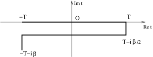
Figure 1: The contour $C$ in the complex time plane used here for the real time formulation.

In this section we review the real time formulation of equilibrium thermal field theory leading to the spectral representations of bosonic two-point functions MS . This formulation begins with a comparison between the time evolution operator $e^{-iH(t_{2}-t_{1})}$ of quantum theory and the Boltzmann weight $e^{-\beta H}=e^{-iH(\tau-i\beta-\tau)}$ of statistical physics, where we introduce $\tau$ as a complex variable. Thus while for the time evolution operator, the times $t_{1}$ and $t_{2}$ $~{}(t_{2}>t_{1})$ are any two points on the real line, the Boltzmann weight involves a path from $\tau$ to $\tau-i\beta$ in the complex time plane. Setting this $\tau=-T$, where $T$ is real, positive and large, we can get the contour $C$ shown in Fig. 1, lying within the region of analyticity in this plane and accommodating real time correlation functions Mills ; Niemi .

Let a general bosonic interacting field in the Heisenberg representation be denoted by $\Phi_{l}(x)$, whose subscript $l$ collects the index (or indices) denoting the field component and derivatives acting on it. Although we shall call its two-point function as propagator, $\Phi_{l}(x)$ can be an elementary field or a composite local operator. (If $\Phi_{l}(x)$ denotes the pion field, it will, of course, not have any index).

The thermal expectation value of the product $\Phi_{l}(x)\Phi^{\dagger}_{l^{\prime}}(x^{\prime})$ may be expressed as

$$\langle\Phi_{l}(x)\Phi^{\dagger}_{l^{\prime}}(x^{\prime})\rangle=\frac{1}{Z}\sum_{m,n}e^{-\beta E_{m}}\langle m|\Phi_{l}(x)|n\rangle\langle n|\Phi^{\dagger}_{l^{\prime}}(x^{\prime})|m\rangle\,,$$ (2.1)

where $\langle O\rangle$ for any operator $O$ denotes equilibrium ensemble average;

$$\langle O\rangle={\rm Tr}(e^{-\beta H}O)/Z\,,~{}~{}~{}~{}~{}~{}~{}~{}Z=Tre^{-\beta H}\,.$$ (2.2)

Note that we have two sums in (2.1), one to evaluate the trace and the other to separate the field operators. They run over a complete set of states, which we choose as eigenstates $|m\rangle$ of four-momentum $P_{\mu}$. Using translational invariance of the field operator,

$$\Phi_{l}(x)=e^{iP\cdot x}\Phi_{l}(0)e^{-iP\cdot x}\,,$$ (2.3)

we get

$$\langle\Phi_{l}(x)\Phi^{\dagger}_{l^{\prime}}(x^{\prime})\rangle=\frac{1}{Z}\sum_{m,n}e^{-\beta E_{m}}\,e^{i(k_{m}-k_{n})\cdot(x-x^{\prime})}\langle m|\Phi_{l}(0)|n\rangle\langle n|\Phi^{\dagger}_{l^{\prime}}(0)|m\rangle\,.$$ (2.4)

Its spatial Fourier transform is

$$\!\!\!\!\!\!\!\!\int d^{3}x\,e^{-i\boldsymbol{k}\cdot(\boldsymbol{x}-\boldsymbol{x}^{\prime})}\langle\Phi_{l}(x)\Phi^{\dagger}_{l^{\prime}}(x^{\prime})\rangle$$

$$\!\!\!\!\!\!\!\!=\frac{(2\pi)^{3}}{Z}\sum_{m,n}e^{-\beta E_{m}}\,e^{i(E_{m}-E_{n})(\tau-\tau^{\prime})}\delta^{3}(\boldsymbol{k}_{m}-\boldsymbol{k}_{n}+\boldsymbol{k})\langle m|\Phi_{l}(0)|n\rangle\langle n|\Phi^{\dagger}_{l^{\prime}}(0)|m\rangle\,,$$ (2.5)

where the times $\tau,\,\tau^{\prime}$ are on the contour $C$. We now insert unity on the left of eq. (2.5) in the form

$$1=\int_{-\infty}^{\infty}dk_{0}^{\prime}\delta(E_{m}-E_{n}+k_{0}^{\prime})\,.$$

(We reserve $k_{0}$ for the variable conjugate to the real time.) Then it may be written as

$$\int d^{3}x\,e^{-i\boldsymbol{k}\cdot(\boldsymbol{x}-\boldsymbol{x}^{\prime})}\langle\Phi_{l}(x)\Phi^{\dagger}_{l^{\prime}}(x^{\prime})\rangle=\int\frac{dk_{0}^{\prime}}{2\pi}e^{-ik_{0}^{\prime}(\tau-\tau^{\prime})}M^{+}_{ll^{\prime}}(k_{0}^{\prime},\boldsymbol{k})\,,$$ (2.6)

where the spectral function $M^{+}$ is given by $[k^{\prime}_{\mu}=(k_{0}^{\prime},\boldsymbol{k})]$

$$M^{+}_{ll^{\prime}}(k^{\prime})=\frac{(2\pi)^{4}}{Z}\sum_{m,n}e^{-\beta E_{m}}\,\delta^{4}(k_{m}-k_{n}+k^{\prime})\langle m|\Phi_{l}(0)|n\rangle\langle n|\Phi^{\dagger}_{l^{\prime}}(0)|m\rangle\,.$$ (2.7)

In just the same way, we can work out the Fourier transform of $\langle\Phi^{\dagger}_{l^{\prime}}(x^{\prime})\Phi_{l}(x)\rangle$

$$\int d^{3}x\,e^{-i\boldsymbol{k}\cdot(\boldsymbol{x}-\boldsymbol{x}^{\prime})}\langle\Phi^{\dagger}_{l^{\prime}}(x^{\prime})\Phi_{l}(x)\rangle=\int\frac{dk_{0}^{\prime}}{2\pi}e^{-ik_{0}^{\prime}(\tau-\tau^{\prime})}M^{-}_{ll^{\prime}}(k_{0}^{\prime},\boldsymbol{k})\,,$$ (2.8)

with a second spectral function $M^{-}$ is given by

$$M^{-}_{ll^{\prime}}(k^{\prime})=\frac{(2\pi)^{4}}{Z}\sum_{m,n}e^{-\beta E_{m}}\,\delta^{4}(k_{n}-k_{m}+k^{\prime})\langle m|\Phi^{\dagger}_{l^{\prime}}(0)|n\rangle\langle n|\Phi_{l}(0)|m\rangle\,.$$ (2.9)

The two spectral functions are related by the KMS relation Kubo ; Martin

$$M^{+}_{ll^{\prime}}(k)=e^{\beta k_{0}}M_{ll^{\prime}}^{-}(k)\,,$$ (2.10)

in momentum space, which may be obtained simply by interchanging the dummy indices $m,n$ in one of $M^{\pm}_{ll^{\prime}}(k)$ and using the energy conserving $\delta$-function.

We next introduce the difference of the two spectral functions,

$$\rho_{ll^{\prime}}(k)\equiv M_{ll^{\prime}}^{+}(k)-M_{ll^{\prime}}^{-}(k)\,,$$ (2.11)

and solve this identity and the KMS relation (2.10) for $M^{\pm}_{ll^{\prime}}(k)$,

$$M^{+}_{ll^{\prime}}(k)=\{1+f(k_{0})\}\rho_{ll^{\prime}}(k)\,,~{}~{}~{}~{}M^{-}_{ll^{\prime}}(k)=f(k_{0})\rho_{ll^{\prime}}(k)\,,$$ (2.12)

where $f(k_{0})$ is the distribution-like function

$$f(k_{0})=\frac{1}{e^{\beta k_{0}}-1}\,,~{}~{}~{}~{}~{}~{}~{}~{}-\infty<k_{0}<\infty\,.$$ (2.13)

In terms of the true distribution function

$$n(|k_{0}|)=\frac{1}{e^{\beta|k_{0}|}-1}\,,$$ (2.14)

it may be expressed as

$$f(k_{0}) = f(k_{0})\{\theta(k_{0})+\theta(-k_{0})\}$$ (2.15)

$$= n\epsilon(k_{0})-\theta(-k_{0})\,.$$

With the above ingredients, we can build the spectral representations for the two types of thermal propagators. First consider the time-ordered one,

$$-iD_{ll^{\prime}}(x,x^{\prime}) = \langle T_{c}\Phi_{l}(x)\Phi^{\dagger}_{l^{\prime}}(x^{\prime})\rangle$$ (2.16)

$$= \theta_{c}(\tau-\tau^{\prime})\langle\Phi_{l}(x)\Phi^{\dagger}_{l^{\prime}}(x^{\prime})\rangle+\theta_{c}(\tau^{\prime}-\tau)\langle\Phi^{\dagger}_{l^{\prime}}(x^{\prime})\Phi_{l}(x)\rangle\,.$$

Using eqs. (2.6,2.8,2.12), we see that its spatial Fourier transform is given by Mills

$$D_{ll^{\prime}}(\tau-\tau^{\prime},\boldsymbol{k})=i\int_{-\infty}^{\infty}\frac{dk_{0}^{\prime}}{2\pi}\rho_{ll^{\prime}}(k_{0}^{\prime},\boldsymbol{k})e^{-ik_{0}^{\prime}(\tau-\tau^{\prime})}\{\theta_{c}(\tau-\tau^{\prime})+f(k_{0}^{\prime})\}\,,$$ (2.17)

As $T\rightarrow\infty$, the contour of Fig. 1 simplifies, reducing essentially to two parallel lines, one the real axis and the other shifted by $-i\beta/2$, points on which will be denoted respectively by subscripts 1 and $2$, so that $\tau_{1}=t,\,\tau_{2}=t-i\beta/2$ Niemi . The propagator then consists of four pieces, which may be put in the form of a $2\times 2$ matrix. The contour ordered $\theta^{\prime}s$ may now be converted to the usual time ordered ones. If $\tau,\tau^{\prime}$ are both on line $1$ (the real axis), the $\tau$ and $t$ orderings coincide, $\theta_{c}(\tau_{1}-\tau^{\prime}_{1})=\theta(t-t^{\prime})$. If they are on two different lines, the $\tau$ ordering is definite, $\theta_{c}(\tau_{1}-\tau^{\prime}_{2})=0,\,\theta_{c}(\tau_{2}-\tau^{\prime}_{1})=1$. Finally if they are both on line $2$, the two orderings are opposite, $\theta_{c}(\tau_{2}-\tau^{\prime}_{2})=\theta(t^{\prime}-t)$.

Back to real time, we can work out the usual temporal Fourier transform of the components of the matrix to get

$$\boldsymbol{D}_{ll^{\prime}}(k_{0},\boldsymbol{k})=\int_{-\infty}^{\infty}\frac{dk_{0}^{\prime}}{2\pi}\rho_{ll^{\prime}}(k_{0}^{\prime},\boldsymbol{k})\boldsymbol{\Lambda}(k_{0}^{\prime},k_{0})\,,$$ (2.18)

where the elements of the matrix $\boldsymbol{\Lambda}$ are given by MS

$$\Lambda_{11}=-\Lambda_{22}^{*}=\frac{1}{k_{0}^{\prime}-k_{0}-i\eta}+2\pi if(k_{0}^{\prime})\delta(k_{0}^{\prime}-k_{0})\,,$$

$$\Lambda_{12}=\Lambda_{21}=2\pi ie^{\beta k_{0}^{\prime}/2}f(k_{0}^{\prime})\delta(k_{0}^{\prime}-k_{0})\,.$$ (2.19)

Using relation (2.15), we may rewrite (2.19) in terms of $n$,

$$\Lambda_{11}=-\Lambda_{22}^{*}=\frac{1}{k_{0}^{\prime}-k_{0}-i\eta\epsilon(k_{0})}+2\pi in\epsilon(k_{0})\delta(k_{0}^{\prime}-k_{0})\,,$$

$$\Lambda_{12}=\Lambda_{21}=2\pi i\sqrt{n(1+n)}\epsilon(k_{0})\delta(k_{0}^{\prime}-k_{0})\,.$$ (2.20)

The matrix $\boldsymbol{\Lambda}$ and hence the propagator $\boldsymbol{D}_{ll^{\prime}}$ can be diagonalised to give

$$\boldsymbol{D}_{ll^{\prime}}(k_{0},\boldsymbol{k})=\boldsymbol{U}\left(\begin{array}[]{cc}\overline{D}_{ll^{\prime}}&0\\ 0&-\overline{D}_{ll^{\prime}}^{\,*}\end{array}\right)\boldsymbol{U}\,,$$ (2.21)

where $\overline{D}_{ll^{\prime}}$ and $\boldsymbol{U}$ are given by

$$\overline{D}_{ll^{\prime}}(k_{0},\boldsymbol{k})=\int_{-\infty}^{\infty}\frac{dk_{0}^{\prime}}{2\pi}\frac{\rho_{ll^{\prime}}(k_{0}^{\prime},\boldsymbol{k})}{k_{0}^{\prime}-k_{0}-i\eta\epsilon(k_{0})}\,,~{}~{}~{}~{}~{}~{}\boldsymbol{U}=\left(\begin{array}[]{cc}\sqrt{1+n}&\sqrt{n}\\ \sqrt{n}&\sqrt{1+n}\end{array}\right)\,.$$ (2.22)

Eq. (2.21) shows that $\overline{D}$ can be obtained from any of the elements of the matrix $\boldsymbol{D}$, say $D_{11}$. Omitting the indices $ll^{\prime}$, we get

$${\rm Re}\overline{D}={\rm ReD}_{11}\,,~{}~{}~{}~{}{\rm Im}\overline{D}=\tanh(\beta|k_{0}|/2){\rm ImD}_{11}\,.$$ (2.23)

Looking back at the spectral functions $M^{\pm}_{ll^{\prime}}$ defined by (2.7, 2.9), we can express them as usual four-dimensional Fourier transforms of ensemble average of the operator products, so that $\rho_{ll^{\prime}}$ is the Fourier transform of that of the commutator,

$$\rho_{ll^{\prime}}(k_{0},\boldsymbol{k})=\int d^{4}ye^{ik\cdot(y-y^{\prime})}\langle[\Phi_{l}(y),\Phi_{l^{\prime}}(y^{\prime})]\rangle\,,$$ (2.24)

where the time components of $y$ and $y^{\prime}$ are on the real axis in the $\tau$-plane. Taking the spectral function for the free scalar field,

$$\rho_{0}=2\pi\epsilon(k_{0})\delta(k^{2}-m^{2})\,,$$ (2.25)

we see that $\overline{D}$ becomes the free propagator, $\overline{D}(k_{0},\boldsymbol{k})=-1/(k^{2}-m^{2})$.

We next consider the retarded thermal propagator

$$D^{R}_{ll^{\prime}}(x,x^{\prime})=i\theta_{c}(\tau-\tau^{\prime})\langle[\Phi_{l}(\boldsymbol{x},\tau),\Phi_{l^{\prime}}(\boldsymbol{x}^{\prime},\tau^{\prime})]\rangle\,,$$ (2.26)

where again $\tau\,,\tau^{\prime}$ are on the contour $C$ (Fig. 1). Noting eqs. (2.6,2.8,2.11) the three dimensional Fourier transform may immediately be written as

$$D^{R}_{ll^{\prime}}(\tau-\tau^{\prime},\boldsymbol{k})=i\theta_{c}(\tau-\tau^{\prime})\int_{-\infty}^{\infty}\frac{dk_{0}^{\prime}}{2\pi}e^{-ik_{0}^{\prime}(\tau-\tau^{\prime})}\rho_{ll^{\prime}}(k_{0}^{\prime},\boldsymbol{k})\,.$$ (2.27)

As before we isolate the different components with real times and take the Fourier transform with respect to real time. Thus for the $11$-component we simply have

$$D^{R}_{ll^{\prime}}(t-t^{\prime},\boldsymbol{k})_{11}=i\theta(t-t^{\prime})\int_{-\infty}^{\infty}\frac{dk_{0}^{\prime}}{2\pi}e^{-ik_{0}^{\prime}(t-t^{\prime})}\rho_{ll^{\prime}}(k_{0}^{\prime},\boldsymbol{k})\,,$$ (2.28)

whose temporal Fourier transform gives

$$D^{R}_{ll^{\prime}}(k_{0},\boldsymbol{k})_{11}=\int_{-\infty}^{\infty}\frac{dk_{0}^{\prime}}{2\pi}\frac{\rho_{ll^{\prime}}(k_{0}^{\prime},\boldsymbol{k})}{k_{0}^{\prime}-k_{0}-i\eta}\,.$$ (2.29)

This $11$-component suffices for us, but we also display the complete matrix,

$$\boldsymbol{D}^{R}_{ll^{\prime}}(k_{0},\boldsymbol{k})=\left(\begin{array}[]{cc}D^{R}_{ll^{\prime}}(k)_{11}&0\\ \rho_{ll^{\prime}}(k)\{\sqrt{\frac{n}{n+1}}\theta(k_{0})+\sqrt{\frac{n+1}{n}}\theta(-k_{0})\}&-D^{R*}_{ll^{\prime}}(k)_{11}\end{array}\right)\,.$$ (2.30)

Though we deal with matrices in real time formulation, it is the $11$-component that is physical. Eqs. (2.22) and (2.29) then show that we can continue the time-ordered two-point function into the retarded one by simply changing the $i\epsilon$ prescription,

$$D^{R}_{ll^{\prime}}(k_{0}+i\eta,\boldsymbol{k})_{11}=\overline{D}_{ll^{\prime}}(k_{0}+i\eta\epsilon(q_{0})\to k_{0}+i\eta,\boldsymbol{k})\,.$$ (2.31)

The point to note here is that for the time-ordered propagator, it is the diagonalised matrix and not the matrix itself, whose $11$-component can be continued in a simple way.

II.2 Transport coefficients

We now use the linear response approach to arrive at expressions of the transport coefficients as integrals of retarded Green’s functions over space. We follow the method proposed by Zubarev Zubarev , which is excellently reviewed in Hosoya . Here the system is supposed to be in the hydrodynamical stage where the mean free time of the constituent particles is much shorter than the relaxation time of the whole system under consideration. Thus local equilibrium will be attained quickly, while global equilibrium will be approaching gradually. Since the system is assumed to be not far from equilibrium, we may retain only linear terms in space-time gradients of thermodynamical parameters, like temperature and velocity fields. We assume the energy-momentum of the system to be conserved,

$$\partial_{\mu}T^{\mu\nu}(\boldsymbol{x},t)=0~{}.$$ (2.32)

The non-equilibrium density matrix operator is constructed in the Heisenberg picture, where it is independent of time,

$$\frac{d\rho}{dt}=0~{}.$$ (2.33)

Following Zubarev, we construct the operator $B(\boldsymbol{x},t)$,

$$B(\boldsymbol{x},t)=\epsilon\int_{-\infty}^{t}dt_{1}e^{\epsilon(t_{1}-t)}F^{\nu}(\boldsymbol{x},t_{1})T_{0\nu}(\boldsymbol{x},t_{1})~{},~{}~{}~{}~{}(\epsilon\to 0^{+})$$ (2.34)

where $F^{\nu}(\boldsymbol{x},t)=\beta(\boldsymbol{x},t)u^{\nu}(\boldsymbol{x},t)$. Here $\beta(\boldsymbol{x},t)$ is a Lorentz invariant quantity defining the local temperature and $u^{\nu}(\boldsymbol{x},t)$ is the four-velocity field of the fluid,

$$u^{\nu}(\boldsymbol{x},t)u_{\nu}(\boldsymbol{x},t)=1~{}.$$ (2.35)

The construction (2.34), which smooths out the oscillating terms resemble the one used in the formal theory of scattering Zubarev ; Gell-Mann and selects out the retarded solution.

The expression (2.34) is actually independent of $t$; the time derivative is

$$\frac{d}{dt}B(\boldsymbol{x},t)=\epsilon F^{\nu}(\boldsymbol{x},t)T_{0\nu}(\boldsymbol{x},t)-\epsilon^{2}\int_{-\infty}^{t}dt_{1}e^{\epsilon(t_{1}-t)}F^{\nu}(\boldsymbol{x},t_{1})T_{0\nu}(\boldsymbol{x},t_{1})~{}.$$ (2.36)

As $T_{0\nu}$ and $F^{\nu}$ are finite, the right hand side of (2.36) goes to zero as $\epsilon\to 0$. Also integrating (2.34) by parts, we get

$$B(\boldsymbol{x},t)=F^{\nu}(\boldsymbol{x},t)T_{0\nu}(\boldsymbol{x},t)-\int_{-\infty}^{t}dt_{1}e^{\epsilon(t_{1}-t)}\left(F^{\nu}\frac{dT_{0\nu}}{dt}+\frac{dF^{\nu}}{dt}T_{0\nu}\right)~{}.$$ (2.37)

We now consider the space integral of (2.37). Using the energy-momentum conservation rule (2.32), we integrate the second term in (2.37) by parts and neglect the surface integrals to get

$$\int d^{3}xB(\boldsymbol{x},t) = \int d^{3}xF^{\nu}(\boldsymbol{x},t)T_{0\nu}(\boldsymbol{x},t)$$ (2.38)

$$- \int d^{3}x\int_{-\infty}^{t}dt_{1}e^{\epsilon(t_{1}-t)}T_{{\mu\nu}}(\boldsymbol{x},t_{1})\partial^{\mu}F^{\nu}(\boldsymbol{x},t_{1})$$

$$\equiv A-B$$

where we have abbreviated the first and second terms by $A$ and $-B$ respectively. Then the non-equilibrium statistical density matrix is given by

$$\rho=e^{-A+B}/{\rm Tr}e^{-A+B}~{}.$$ (2.39)

The first term $A$ in eq. (2.38) characterises local equilibrium,

$$\rho_{0}=e^{-A}/{\rm Tr}e^{-A}$$ (2.40)

while the second term $B$ including the thermodynamical force $\partial^{\mu}F^{\nu}$ describes deviation from equilibrium.

In order to expand $\rho$ in a series in $B$ we define the function

$$Q(\tau)=e^{-(1-\tau)A}e^{\tau(-A+B)}$$ (2.41)

such that the boundary conditions at $\tau=0$ and $\tau=1$ correspond to the equilibrium and non-equilibrium density matrices,

$$Q(\tau=0)=e^{-A}=\rho_{0}~{},~{}~{}~{}~{}Q(\tau=1)=e^{-A+B}=\rho~{}.$$ (2.42)

We then differentiate $Q(\tau)$ w.r.t $\tau$ to get

$$\frac{dQ(\tau)}{d\tau}=e^{-(1-\tau)A}Be^{(1-\tau)A}Q(\tau)$$ (2.43)

which can be integrated to give

$$Q(\tau)=Q(0)+\int_{0}^{\tau}d\tau^{\prime}e^{-(1-\tau^{\prime})A}Be^{(1-\tau^{\prime})A}Q(\tau^{\prime})~{}.$$ (2.44)

It can be solved iteratively. Keeping up to the first order term (linear response) and setting $\tau=1$ we get the required result

$$\rho=\rho_{0}\left[1+\int_{0}^{1}e^{-\tau A}Be^{\tau A}\right]~{}.$$ (2.45)

Applying this formula to the energy-momentum tensor, we get its response to the thermodynamical forces as Hosoya

$$\langle T_{{\mu\nu}}(\boldsymbol{x},t)\rangle = \langle T_{{\mu\nu}}(\boldsymbol{x},t)\rangle_{0}$$ (2.46)

$$+ \int d^{3}x^{\prime}\int_{-\infty}^{t}dt^{\prime}e^{\epsilon(t_{1}-t)}(T_{{\mu\nu}}(\boldsymbol{x},t),T_{\rho\sigma}(\boldsymbol{x}^{\prime},t^{\prime}))\partial^{\rho}F^{\sigma}(\boldsymbol{x}^{\prime},t^{\prime})$$

where

$$(T_{{\mu\nu}}(\boldsymbol{x},t),T_{\rho\sigma}(\boldsymbol{x}^{\prime},t^{\prime})) = \int_{0}^{1}d\tau\left\{\langle T_{{\mu\nu}}(\boldsymbol{x},t)e^{-\tau A}T_{\rho\sigma}(\boldsymbol{x}^{\prime},t^{\prime})e^{\tau A}\rangle_{0}\right.$$ (2.47)

$$\left.-\langle T_{{\mu\nu}}(\boldsymbol{x},t)\rangle_{0}\langle T_{\rho\sigma}(\boldsymbol{x}^{\prime},t^{\prime})\rangle_{0}\right\}$$

is the correlation function to be evaluated. As the correlation is assumed to vanish as $t^{\prime}\to-\infty$, it can be put in terms of the conventional retarded Green’s function. Omitting indices it is

$$(T(\boldsymbol{x},t),T(\boldsymbol{x}^{\prime},t^{\prime}))=\frac{1}{\beta}\int_{-\infty}^{t}dt^{\prime}\langle T(\boldsymbol{x},t),T(\boldsymbol{x}^{\prime},t^{\prime})\rangle_{ret}$$ (2.48)

with

$$\langle T(\boldsymbol{x},t),T(\boldsymbol{x}^{\prime},t^{\prime})\rangle_{ret}\equiv i\theta(t-t^{\prime})\langle[T(\boldsymbol{x},t),T(\boldsymbol{x}^{\prime},t^{\prime})]\rangle_{0}$$ (2.49)

We now use eq. (2.46) to obtain the expectation value of the viscous-shear stress part of the non-equilibrium energy momentum tensor which is given by

$$T^{\mu\nu}=T^{{\mu\nu}\,(0)}+\pi^{\mu\nu}+(P^{\mu}u^{\nu}+P^{\nu}u^{\mu})$$ (2.50)

where $T^{{\mu\nu}\,(0)}=(\epsilon+p)u^{\mu}u^{\nu}-g^{\mu\nu}p$ is the equilibrium part, $\pi^{\mu\nu}$ is the viscous-shear stress tensor and $P^{\mu}$ is the heat current. Also, with a view to separate scalar, vector and tensor processes the quantity $T_{\rho\sigma}\partial^{\rho}F^{\sigma}$ in (2.38) is expanded as

$$T_{\rho\sigma}\partial^{\rho}F^{\sigma}=\beta\pi_{\rho\sigma}\partial^{\rho}u^{\sigma}+\beta P_{\rho}(\beta\partial^{\rho}\beta+u\cdot\partial u^{\rho})-\beta\widetilde{p}\partial\cdot u$$ (2.51)

with $\widetilde{p}=p-c_{s}^{2}\epsilon$, $c_{s}$ being the sound velocity. Using now the fact that the correlation function between operators of different ranks vanish in an isotropic medium, one can write from (2.46)

$$\langle\pi_{{\mu\nu}}(\boldsymbol{x},t)\rangle = \langle\pi_{{\mu\nu}}(\boldsymbol{x},t)\rangle_{0}$$ (2.52)

$$+ \int d^{3}x^{\prime}\int_{-\infty}^{t}dt^{\prime}e^{\epsilon(t_{1}-t)}(\pi_{{\mu\nu}}(\boldsymbol{x},t),\pi_{\rho\sigma}(\boldsymbol{x}^{\prime},t^{\prime}))\beta(\boldsymbol{x}^{\prime},t^{\prime})\partial^{\rho}u^{\sigma}(\boldsymbol{x}^{\prime},t^{\prime})$$

with $\langle\pi_{\mu\nu}(\boldsymbol{x},t)\rangle_{0}=0$. Following Hosoya Hosoya we write the correlation function as

$$(\pi_{{\mu\nu}},\pi_{\rho\sigma})=\frac{1}{10}[\Delta_{\mu\rho}\Delta_{\nu\sigma}+\Delta_{\mu\sigma}\Delta_{\nu\rho}-\frac{2}{3}\Delta_{\mu\nu}\Delta_{\rho\sigma}](\pi^{\alpha\beta},\pi_{\alpha\beta})$$ (2.53)

where $\Delta_{\mu\nu}=g_{\mu\nu}-u_{\mu}u_{\nu}$. Assuming now that changes in the thermodynamic forces are small over the correlation length of the two point function, the factor $\beta\partial^{\rho}u^{\sigma}$ can be taken out of the integral giving finally

$$\langle\pi^{\mu\nu}(\boldsymbol{x},t)\rangle=\eta[\Delta^{\mu}_{\rho}\Delta^{\nu}_{\sigma}(\partial^{\rho}u^{\sigma}+\partial^{\sigma}u^{\rho})-\frac{2}{3}\Delta^{\mu\nu}\Delta_{\rho\sigma}\partial^{\rho}u^{\sigma}]$$ (2.54)

where

$$\eta = \frac{1}{10}\int_{-\infty}^{0}dt_{1}e^{\epsilon(t_{1}-t)}\int_{-\infty}^{t_{1}}dt^{\prime}\,\int d^{3}x^{\prime}\,\langle\pi^{\alpha\beta}(\boldsymbol{x},t),\pi_{\alpha\beta}(\boldsymbol{x}^{\prime},t^{\prime})\rangle_{ret}$$ (2.55)

$$= \frac{1}{10}\int_{-\infty}^{0}dt_{1}e^{\epsilon t_{1}}\int_{-\infty}^{t_{1}}dt^{\prime}\,i\int d^{3}x^{\prime}\,\theta(-t^{\prime})\langle[\pi^{\alpha\beta}(0,0),\pi_{\alpha\beta}(\boldsymbol{x}^{\prime},t^{\prime})]\rangle_{0}~{};~{}~{}~{}~{}~{}~{}(\boldsymbol{x}\to 0,t\to 0).$$

Again, starting with the pressure $p(\boldsymbol{x},t)$ on the l.h.s of eq. (2.46) and following the steps as described above we obtain

$$\langle p(\boldsymbol{x},t)\rangle=\langle p(\boldsymbol{x},t)\rangle_{0}-\zeta\partial_{\rho}u^{\rho}(\boldsymbol{x},t)~{}.$$ (2.56)

where the bulk viscosity $\zeta$ is given in terms of a retarded correlation function by

$$\zeta=\int_{-\infty}^{0}dt_{1}e^{\epsilon(t_{1}-t)}\int_{-\infty}^{t_{1}}dt^{\prime}\,\int d^{3}x^{\prime}\,\langle\widetilde{p}(\boldsymbol{x},t),\widetilde{p}(\boldsymbol{x}^{\prime},t^{\prime})\rangle_{ret}~{}.$$ (2.57)

Here $\widetilde{p}(\boldsymbol{x},t)=p(\boldsymbol{x},t)-c_{s}^{2}\epsilon(\boldsymbol{x},t)$ with $\epsilon(\boldsymbol{x},t)$ the energy density and $c_{s}^{2}=\langle\partial p/\partial\epsilon\rangle_{0}$.

Recall that $\langle\cdots\rangle_{0}$ denotes equilibrium ensemble average. From now on we shall drop the subscript ’0’ on the correlation functions.

II.3 Perturbative evaluation

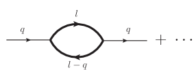
Figure 2: The first term in the so-called skeleton expansion of the two-point function. Heavy lines denote full propagators.

Clearly the spectral forms and their inter-relations derived in Sec. IIA hold also for the two-point function appearing in eq. (2.55) for the shear viscosity. We begin with four-dimensional Fourier transforms. To calculate the $11$-element of the the retarded two-point function

$$\Pi_{11}^{R}(q)=i\int d^{4}xe^{iq(x-x^{\prime})}\theta(t-t^{\prime})\langle[\pi_{\alpha\beta}(\boldsymbol{x},t),\pi^{\alpha\beta}(\boldsymbol{x}^{\prime},t^{\prime})]\rangle\,,$$ (2.58)

we consider the corresponding time-ordered one,

$$\Pi_{11}(q)=i\int d^{4}xe^{iq(x-x^{\prime})}\langle T\pi_{\alpha\beta}(\boldsymbol{x},t)\pi^{\alpha\beta}(\boldsymbol{x}^{\prime},t^{\prime})\rangle\,,$$ (2.59)

which can be calculated perturbatively. The viscous stress tensor can be extracted from the energy momentum tensor using the formula

$$\pi_{\alpha\beta}(x)=(\Delta_{\alpha}^{\rho}\Delta_{\beta}^{\sigma}-\frac{1}{3}\Delta_{\alpha\beta}\Delta^{\rho\sigma})T_{\rho\sigma}(x)$$ (2.60)

where $T_{\mu\nu}=-g_{\mu\nu}{\cal L}+\frac{\partial{\cal L}}{\partial(\partial^{\mu}\vec{\phi})}\cdot{\partial_{\nu}\vec{\phi}}$ in which $\vec{\phi}(x)$ denotes the pion triplet. We take the lowest order chiral Lagrangian given by Gasser

$${\cal L} = \frac{1}{2}\partial_{\mu}\vec{\phi}\cdot\partial^{\mu}\vec{\phi}-\frac{1}{2}m_{\pi}^{2}\vec{\phi}\cdot\vec{\phi}+{\cal L}_{int}$$

$${\cal L}_{int} = -\frac{1}{6f_{\pi}^{2}}[\partial_{\mu}\vec{\phi}\cdot\partial^{\mu}\vec{\phi}\,\vec{\phi}\cdot\vec{\phi}-\vec{\phi}\cdot\partial_{\mu}\vec{\phi}\,\vec{\phi}\cdot\partial^{\mu}\vec{\phi}]+\frac{m_{\pi}^{2}}{4!~{}f_{\pi}^{2}}(\vec{\phi}\cdot\vec{\phi})^{2}~{}.$$ (2.61)

The time-ordered correlator, to leading order, is then given by Wick contractions of pion fields in $\pi_{\alpha\beta}$ which is obtained as

$$\pi_{\alpha\beta}(x)=(\Delta_{\alpha}^{\rho}\Delta_{\beta}^{\sigma}-\frac{1}{3}\Delta_{\alpha\beta}\Delta^{\rho\sigma})\partial_{\rho}\vec{\phi}(x)\cdot\partial_{\sigma}\vec{\phi}(x)~{}.$$ (2.62)

In the so-called skeleton expansion, these contractions are expressed in terms of complete propagators (see Fig. 2) to get,

$$\Pi_{11}(q)=i\int\frac{d^{4}l}{(2\pi)^{4}}N(l,q)D_{11}(l)D_{11}(l-q)\,,$$ (2.63)

where $D_{11}$ is given by eq. (2.18) and $N(l,q)$ is determined by the derivatives acting on the pion fields,

$$N(l,q)=-g_{\pi}\,[\boldsymbol{l}^{2}(\boldsymbol{l}-\boldsymbol{q})^{2}+\frac{1}{3}\{\boldsymbol{l}\cdot(\boldsymbol{l}-\boldsymbol{q})\}^{2}]$$ (2.64)

where the pion isospin degeneracy factor $g_{\pi}=3$.

To work out the $l_{0}$ integral in eq. (2.63), it is more convenient to use $\Lambda_{11}$ given by eq. (2.19) than by eq. (2.20). Closing the contour in the upper or lower half $l_{0}$-plane we get

$$\Pi_{11}(q)=\int\frac{d^{3}l}{(2\pi)^{3}}N(\boldsymbol{l},\boldsymbol{q})\int\frac{dk_{0}^{\prime}}{2\pi}\rho(k_{0}^{\prime},\boldsymbol{l})\frac{dk_{0}^{\prime\prime}}{2\pi}\rho(k_{0}^{\prime\prime},\boldsymbol{l}-\boldsymbol{q})K(q_{0},k_{0}^{\prime},k_{0}^{\prime\prime})\,,$$ (2.65)

where

$$K=\frac{\{1+f(k_{0}^{\prime})\}f(k_{0}^{\prime\prime})}{q_{0}-(k_{0}^{\prime}-k_{0}^{\prime\prime})+i\eta}-\frac{f(k_{0}^{\prime})\{1+f(k_{0}^{\prime\prime})\}}{q_{0}-(k_{0}^{\prime}-k_{0}^{\prime\prime})-i\eta}\,.$$ (2.66)

The imaginary part of $\Pi_{11}$ arises from the factor $K$,

$${\rm Im}K = -\pi\left[\{1+f(k_{0}^{\prime})\}f(k_{0}^{\prime\prime})+f(k_{0}^{\prime})\{1+f(k_{0}^{\prime\prime})\}\right]\delta(q_{0}-(k_{0}^{\prime}-k_{0}^{\prime\prime}))$$ (2.67)

$$= -\pi\coth(\beta q_{0}/2)\{f(k_{0}^{\prime\prime})-f(k_{0}^{\prime})\}\delta(q_{0}-(k_{0}^{\prime}-k_{0}^{\prime\prime}))\,,$$

while its real part is given by the principal value integrals.

Having obtained the real and imaginary parts of $\Pi_{11}(q)$, we use relations similar to eq. (2.23) to build the $11$-element of the diagonalised $\Pi$ matrix,

$$\overline{\Pi}=\int\frac{d^{3}l}{(2\pi)^{3}}N(\boldsymbol{l},\boldsymbol{q})\int\frac{dk_{0}^{\prime}}{2\pi}\rho(k_{0}^{\prime},\boldsymbol{l})\int\frac{dk_{0}^{\prime\prime}}{2\pi}\rho(k_{0}^{\prime\prime},\boldsymbol{l}-\boldsymbol{q})\frac{\{1+f(k_{0}^{\prime})\}f(k_{0}^{\prime\prime})-f(k_{0}^{\prime})\{1+f(k_{0}^{\prime\prime})\}}{q_{0}-(k_{0}^{\prime}-k_{0}^{\prime\prime})+i\eta\epsilon(q_{0})}\,.$$ (2.68)

Finally $\overline{\Pi}$ can be continued to $\Pi_{11}^{R}$ by a relation similar to eq. (2.30),

$$\Pi^{R}_{11}=\int\frac{d^{3}l}{(2\pi)^{3}}N(\boldsymbol{l},\boldsymbol{q})\int\frac{dk_{0}^{\prime}}{2\pi}\rho(k_{0}^{\prime},\boldsymbol{l})\frac{dk_{0}^{\prime\prime}}{2\pi}\rho(k_{0}^{\prime\prime},\boldsymbol{l}-\boldsymbol{q})\frac{\{1+f(k_{0}^{\prime})\}f(k_{0}^{\prime\prime})-f(k_{0}^{\prime})\{1+f(k_{0}^{\prime\prime})\}}{q_{0}-(k_{0}^{\prime}-k_{0}^{\prime\prime})+i\eta}\,.$$ (2.69)

Note that in eqs. (2.68,2.69) we retain the $f(k_{0}^{\prime})f(k_{0}^{\prime\prime})$ terms in the numerator to put it in a more convenient form. Change the signs of $k_{0}^{\prime}$ and $k_{0}^{\prime\prime}$ in the first and second term respectively. Noting relations like $1+f(-k_{0})=-f(k_{0})$ and $\rho(-k_{0})=-\rho(k_{0})$ we get

$$\Pi^{R}_{11}(q)=\int\frac{d^{3}l}{(2\pi)^{3}}N(\boldsymbol{l},\boldsymbol{q})\int\frac{dk_{0}^{\prime}}{2\pi}\frac{dk_{0}^{\prime\prime}}{2\pi}\rho(k_{0}^{\prime},\boldsymbol{l})\rho(k_{0}^{\prime\prime},\boldsymbol{l}-\boldsymbol{q})f(k_{0}^{\prime})f(k_{0}^{\prime\prime})W(q_{0},k_{0}^{\prime}+k_{0}^{\prime\prime})\,,$$ (2.70)

where

$$W=\frac{1}{q_{0}+k_{0}^{\prime}+k_{0}^{\prime\prime}+i\eta}-\frac{1}{q_{0}-(k_{0}^{\prime}+k_{0}^{\prime\prime})+i\eta}\,.$$ (2.71)

Returning to the expression (2.55) for $\eta$, we now get the three-dimensional spatial integral of the retarded correlation function by setting $\boldsymbol{q}=0$ in eq. (2.58) and Fourier inverting with respect to $q_{0}$,

$$i\int d^{3}x^{\prime}\,\theta(-t^{\prime})\langle[\pi^{\alpha\beta}(\vec{0},0),\pi_{\alpha\beta}(\boldsymbol{x}^{\prime},t^{\prime})]\rangle=-\int dq_{0}\,e^{iq_{0}t^{\prime}}\Pi^{R}_{11}(q_{0},\boldsymbol{q}=0)\,.$$ (2.72)

This completes our use of the real time formulation to get the required result. The integrals appearing in the expression for $\eta$ have been evaluated in Refs. Hosoya ; Lang , which we describe below for completeness.

As shown in Ref. Hosoya , the integral over $t_{1},\,t^{\prime}$ and $q_{0}$ in eqs. (2.55) and (2.72) may be carried out trivially to give

$$\eta=\left.\frac{i}{10}\frac{d}{dq_{0}}\Pi^{R}_{11}(q_{0})\right|_{q_{0}=0}\,.$$ (2.73)

The $q_{0}$ dependence of $\Pi^{R}_{11}$ is contained entirely in $W$,

$$\left.\frac{d}{dq_{0}}W(q_{0})\right|_{q_{0}=0}=-\frac{1}{(k_{0}^{\prime}+k_{0}^{\prime\prime}-i\eta)^{2}}+\frac{1}{(k_{0}^{\prime}+k_{0}^{\prime\prime}+i\eta)^{2}}=2\pi i\delta^{\prime}(k_{0}^{\prime}+k_{0}^{\prime\prime})\,.$$ (2.74)

Changing the integration variables in eq. (2.70) from $k_{0}^{\prime}$, $k_{0}^{\prime\prime}$ to $\overline{k}_{0}=k_{0}^{\prime}+k_{0}^{\prime\prime}$ and $k_{0}=\frac{1}{2}(k_{0}^{\prime}-k_{0}^{\prime\prime})$ we get

$$\eta=\int\frac{d^{3}l}{(2\pi)^{3}}N(\boldsymbol{l})\int\frac{dk_{0}}{(2\pi)^{2}}F(k_{0},\boldsymbol{l})\,,$$ (2.75)

where

$$F(k_{0},\boldsymbol{l})=\left.\frac{d}{d\overline{k}_{0}}\left\{\rho\!\left(\frac{\overline{k}_{0}}{2}+k_{0},\boldsymbol{l}\right)\rho\!\left(\frac{\overline{k}_{0}}{2}-k_{0},\boldsymbol{l}\right)f\!\left(\frac{\overline{k}_{0}}{2}+k_{0}\right)f\!\left(\frac{\overline{k}_{0}}{2}-k_{0}\right)\right\}\right|_{\overline{k}_{0}=0}\,.$$ (2.76)

It turns out that the integral over $k_{0}$ becomes undefined, if we try to evaluate $F(k_{0})$ with the free spectral function $\rho_{0}(k)$ given by eq. (2.25). As pointed out in Ref. Hosoya , we have to take the spectral function for the complete propagator that includes the self-energy of the pion, leading to its finite width $\Gamma$ in the medium,

$$\rho(k_{0},\boldsymbol{l})=\frac{1}{i}\left[\frac{1}{(k_{0}-i\Gamma)^{2}-\omega^{2}}-\frac{1}{(k_{0}+i\Gamma)^{2}-\omega^{2}}\right]\,,~{}~{}~{}~{}~{}~{}~{}~{}~{}~{}\omega=\sqrt{\boldsymbol{l}^{2}+m_{\pi}^{2}}\,.$$ (2.77)

Note that this form of the spectral function trivially follows on replacing $i\eta$ (where $\eta\to 0^{+}$) with $i\Gamma$ in the free spectral function (2.25) which can be written as

$$\rho_{0}(k_{0},\boldsymbol{l})=\frac{1}{i}\left[\frac{1}{(k_{0}-i\eta)^{2}-\omega^{2}}-\frac{1}{(k_{0}+i\eta)^{2}-\omega^{2}}\right]\,.$$ (2.78)

Then $F(k_{0},\boldsymbol{l})$ becomes

$$F=-8\frac{k_{0}^{2}e^{\beta k_{0}}}{(e^{\beta k_{0}}-1)^{2}}\frac{\beta\Gamma^{2}}{\{(k_{0}-i\Gamma)^{2}-\omega^{2}\}^{2}\{(k_{0}+i\Gamma)^{2}-\omega^{2}\}^{2}}\,,$$ (2.79)

having double poles at $k_{0}=2\pi in/\beta$ for $n=\pm 1,\pm 2,\cdots$ and also at $k_{0}=\pm\omega\pm i\Gamma$. The integral over $k_{0}$ may now be evaluated by closing the contour in the upper/lower half-plane to get

$$\int^{+\infty}_{-\infty}\frac{dk_{0}}{(2\pi)^{2}}F(k_{0},\boldsymbol{l})=-\frac{1}{8\pi}\frac{\beta}{\omega^{2}\Gamma}n(\omega)\{1+n(\omega)\}\,,$$ (2.80)

where we retain only the leading (singular) term for small $\Gamma$. In this approximation eq. (2.75) gives

$$\eta=\frac{g_{\pi}\beta}{30\pi^{2}}\int_{0}^{\infty}dl\,\frac{l^{6}}{\omega^{2}\Gamma}{n(\omega)\{1+n(\omega)\}}\,.$$ (2.81)

Proceeding analogously as above, the lowest order contribution to the bulk viscosity can be obtained as Hosoya

$$\zeta=\frac{g_{\pi}\beta}{4\pi^{2}}\int_{0}^{\infty}dl\,\frac{l^{2}(l^{2}/3-c_{s}^{2}\omega^{2})^{2}}{\omega^{2}\Gamma}n(\omega)\{1+n(\omega)\}\,.$$ (2.82)

The width $\Gamma(l)$ at different temperatures is known Goity from chiral perturbation theory. The quantity $\Gamma$ can also be interpreted as the collision frequency, the inverse of which is the relaxation time $\tau$. For collisions of the form $\pi(l)+\pi(k)\to\pi(l^{\prime})+\pi(k^{\prime})$ this is given by(see e.g. Sukanya1 )

$$\Gamma(l)=\tau^{-1}(l)=\int\frac{k^{2}\,dk}{2\pi^{2}\omega_{k}}\frac{\sqrt{s(s-4m_{\pi}^{2})}}{2\omega_{l}}n(\omega_{k})(1+n(\omega_{l^{\prime}}))(1+n(\omega_{k^{\prime}}))\frac{1}{2}\int d\Omega\frac{d\sigma}{d\Omega}$$ (2.83)

where $\frac{d\sigma}{d\Omega}$ is the $\pi\pi$ cross-section. Note that the lowest order formulae for the shear and bulk viscosities obtained above in the linear response approach coincide with the expressions which result from solving the transport equation in the relaxation-time approximation.

III Viscous coefficients in the kinetic theory approach

The kinetic theory approach is suitable for studying transport properties of dilute systems. Here one assumes that the system is characterized by a distribution function which gives the phase space probability density of the particles making up the fluid. Except during collisions, these (on-shell) particles are assumed to propagate classically with well defined position, momenta and energy. It is possible to obtain the non-equilibrium distribution function by solving the transport equation in the hydrodynamic regime by expanding the distribution function in a local equilibrium part along with non-equilibrium corrections. This expansion in terms of gradients of the velocity field is used to linearize the transport equation. The coefficients of expansion which are related to the transport coefficients, satisfy linear integral equations. The standard method of solution involves the use of polynomial functions to reduce these integral equations to algebraic ones.

III.1 Transport coefficients at first Chapman-Enskog order

The evolution of the phase space distribution of the pions is governed by the (transport) equation

$$p^{\mu}\partial_{\mu}f(x,p)=C[f]$$ (3.1)

where $C[f]$ is the collision integral. For binary elastic collisions $p+k\to p^{\prime}+k^{\prime}$ which we consider, this is given by Davesne

$$C[f] = \int d\Gamma_{k}\ d\Gamma_{p^{\prime}}\ d\Gamma_{k^{\prime}}[f(x,p^{\prime})f(x,k^{\prime})\{1+f(x,p)\}\{1+f(x,k)\}$$ (3.2)

$$-f(x,p)f(x,k)\{1+f(x,p^{\prime})\}\{1+f(x,k^{\prime})\}]\ W$$

where the interaction rate,

$$W=\frac{s}{2}\ \frac{d\sigma}{d\Omega}(2\pi)^{6}\delta^{4}(p+k-p^{\prime}-k^{\prime})$$

and $d\Gamma_{q}=\frac{d^{3}q}{(2\pi)^{3}q_{0}}$. The $1/2$ factor comes from the indistinguishability of the initial state pions.

For small deviation from local equilibrium we write, in the first Chapman-Enskog approximation

$$f(x,p)=f^{(0)}(x,p)+\delta f(x,p),~{}~{}~{}\delta f(x,p)=f^{(0)}(x,p)[1+f^{(0)}(x,p)]\phi(x,p)$$ (3.3)

where the equilibrium distribution function (in the new notation) is given by

$$f^{(0)}(x,p)=\left[e^{\frac{p^{\mu}u_{\mu}(x)-\mu_{\pi}(x)}{T(x)}}-1\right]^{-1},$$ (3.4)

with $T(x)$, $u_{\mu}(x)$ and $\mu_{\pi}(x)$ representing the local temperature, flow velocity and pion chemical potential respectively. Putting (3.3) in (3.1) the deviation function $\phi(x,p)$ is seen to satisfy

$$p^{\mu}\partial_{\mu}f^{(0)}(x,p)=-{\cal L}[\phi]$$ (3.5)

where the linearized collision term

$${\cal L}[\phi]= f^{(0)}(x,p)\int d\Gamma_{k}\ d\Gamma_{p^{\prime}}\ d\Gamma_{k^{\prime}}f^{(0)}(x,k)\{1+f^{(0)}(x,p^{\prime})\}\{1+f^{(0)}(x,k^{\prime})\}$$ (3.6)

$$[\phi(x,p)+\phi(x,k)-\phi(x,p^{\prime})-\phi(x,k^{\prime})]\ W~{}.$$

Using the form of $f^{(0)}(x,p)$ as given in (3.4) on the left side of (3.5) and eliminating time derivatives with the help of equilibrium thermodynamic laws we arrive at Sukanya2

$$[Q\partial_{\nu}u^{\nu}+p_{\mu}\Delta^{\mu\nu}(p\cdot u-h)(T^{-1}\partial_{\nu}T-Du_{\nu})-\langle p_{\mu}p_{\nu}\rangle\langle\partial^{\mu}u^{\nu}\rangle]f^{(0)}(1+f^{(0)})=-T{\cal L}[\phi]$$ (3.7)

where $D=u^{\mu}\partial_{\mu}$, $\nabla_{\mu}=\Delta_{\mu\nu}\partial^{\nu}$, $\Delta_{\mu\nu}=g_{\mu\nu}-u_{\mu}u_{\nu}$ and $\langle\cdot\rangle$ indicates a space-like symmetric and traceless combination. In this equation

$$Q=-\frac{1}{3}m_{\pi}^{2}+(p\cdot u)^{2}\{\frac{4}{3}-\gamma^{\prime}\}+p\cdot u\{(\gamma^{\prime\prime}-1)h-\gamma^{\prime\prime\prime}T\}$$ (3.8)

where

$$\gamma^{\prime}=\frac{(S_{2}^{0}/S_{2}^{1})^{2}-(S_{3}^{0}/S_{2}^{1})^{2}+4z^{-1}S_{2}^{0}S_{3}^{1}/(S_{2}^{1})^{2}+z^{-1}S_{3}^{0}/S_{2}^{1}}{(S_{2}^{0}/S_{2}^{1})^{2}-(S_{3}^{0}/S_{2}^{1})^{2}+3z^{-1}S_{2}^{0}S_{3}^{1}/(S_{2}^{1})^{2}+2z^{-1}S_{3}^{0}/S_{2}^{1}-z^{-2}}$$ (3.9)

$$\gamma^{\prime\prime}=1+\frac{z^{-2}}{(S_{2}^{0}/S_{2}^{1})^{2}-(S_{3}^{0}/S_{2}^{1})^{2}+3z^{-1}S_{2}^{0}S_{3}^{1}/(S_{2}^{1})^{2}+2z^{-1}S_{3}^{0}/S_{2}^{1}-z^{-2}}$$ (3.10)

$$\gamma^{\prime\prime\prime}=\frac{S_{2}^{0}/S_{2}^{1}+5z^{-1}S_{3}^{1}/S_{2}^{1}-S_{3}^{0}S_{3}^{1}/(S_{2}^{1})^{2}}{(S_{2}^{0}/S_{2}^{1})^{2}-(S_{3}^{0}/S_{2}^{1})^{2}+3z^{-1}S_{2}^{0}S_{3}^{1}/(S_{2}^{1})^{2}+2z^{-1}S_{3}^{0}/S_{2}^{1}-z^{-2}}$$ (3.11)

with $z=m_{\pi}/T$ and $h=m_{\pi}S_{3}^{1}/S_{2}^{1}$. The functions $S_{n}^{\alpha}(z)$ are integrals over Bose functions Sukanya2 and are defined as $S_{n}^{\alpha}(z)=\sum_{k=1}^{\infty}e^{k\mu_{\pi}/T}k^{-\alpha}K_{n}(kz)$, $K_{n}(x)$ denoting the modified Bessel function of order $n$. The left hand side of (3.5) is thus expressed in terms of thermodynamic forces with different tensorial ranks. In order to be a solution of this equation $\phi$ must also be a linear combination of the corresponding thermodynamic forces. It is typical to take $\phi$ as

$$\phi=A\partial\cdot u+B_{\mu}\nabla^{\mu\nu}(T^{-1}\partial_{\nu}T-Du_{\nu})-C_{\mu\nu}\langle\partial^{\mu}u^{\nu}\rangle$$ (3.12)

which on substitution into (3.7) and comparing coefficients of the (independent) thermodynamic forces on both sides, yields the set of equations

$${\cal L}[A]=-Qf^{(0)}(p)\{1+f^{(0)}(p)\}/T$$ (3.13)

$${\cal L}[C_{\mu\nu}]=-\langle p_{\mu}p_{\nu}\rangle f^{(0)}(p)\{1+f^{(0)}(p)\}/T$$ (3.14)

ignoring the equation for $B_{\mu}$ which is related to thermal conductivity. These integral equations are to be solved to get the coefficients $A$ and $C_{\mu\nu}$. It now remains to link these to the viscous coefficients $\zeta$ and $\eta$. This is achieved by means of the dissipative part of the energy-momentum tensor resulting from the use of the non-equilibrium distribution function (3.3) in

$$T^{\mu\nu}=\int d\Gamma_{p}\ p^{\mu}p^{\nu}f(p)=T^{{\mu\nu}(0)}+\Delta T^{{\mu\nu}}$$ (3.15)

where

$$\Delta T^{\mu\nu}=\int d\Gamma_{p}f^{(0)}(1+f^{(0)})C_{\alpha\beta}\langle p^{\alpha}p^{\beta}\rangle\langle\partial^{\mu}u^{\nu}\rangle+\int d\Gamma_{p}f^{(0)}(1+f^{(0)})QA\Delta^{\mu\nu}\partial_{\sigma}u^{\sigma}~{}.$$ (3.16)

Again, for a small deviation $\phi(x,p)$, close to equilibrium, so that only first order derivatives contribute, the dissipative tensor can be generally expressed in the form Purnendu ; Polak

$$\Delta T^{\mu\nu}=-2\eta\langle\partial^{\mu}u^{\nu}\rangle-\zeta\Delta^{\mu\nu}\partial_{\sigma}u^{\sigma}~{}.$$ (3.17)

Comparing, we obtain the expressions of shear and bulk viscosity,

$$\eta=-\frac{1}{10}\int d\Gamma_{p}\ C_{\mu\nu}\langle p^{\mu}p^{\nu}\rangle f^{(0)}(p)\{1+f^{(0)}(p)\}$$ (3.18)

and

$$\zeta=-\int d\Gamma_{p}\ QAf^{(0)}(p)\{1+f^{(0)}(p)\}~{}.$$ (3.19)

The coefficients $A$ and $C_{\mu\nu}$ are perturbatively obtained from (3.13) and (3.14) by expanding in terms of orthogonal polynomials which reduces the integral equations to algebraic ones. After a tedious calculation using the Laguerre polynomial of 1/2 integral order, the first approximation to the shear and bulk viscosity come out as

$$\eta=\frac{T}{10}\ \frac{\gamma_{0}^{2}}{c_{00}}$$ (3.20)

and

$$\zeta=T\frac{\alpha_{2}^{2}}{a_{22}}$$ (3.21)

where

$$\gamma_{0} = -10\frac{S_{3}^{2}(z)}{S_{2}^{1}(z)}~{},$$

$$c_{00} = 16\{I_{1}(z)+I_{2}(z)+\frac{1}{3}I_{3}(z)\}~{},$$ (3.22)

and

$$\alpha_{2} = \frac{z^{3}}{2}[\frac{1}{3}(\frac{S_{3}^{0}}{S_{2}^{1}}-z^{-1})+(\frac{S_{2}^{0}}{S_{2}^{1}}+\frac{3}{z}\frac{S_{3}^{1}}{S_{2}^{1}})\{(1-\gamma^{\prime\prime})\frac{S_{3}^{1}}{S_{2}^{1}}+\gamma^{\prime\prime\prime}z^{-1}\}$$

$$- (\frac{4}{3}-\gamma^{\prime})\{\frac{S_{3}^{0}}{S_{2}^{1}}+15z^{-2}\frac{S_{3}^{2}}{S_{2}^{1}}+2z^{-1}\}]~{},$$

$$a_{22} = 2z^{2}I_{3}(z)~{}.$$ (3.23)

The integrals $I_{\alpha}(z)$ are given by

$$I_{\alpha}(z) = \frac{z^{4}}{[S_{2}^{1}(z)]^{2}}\ e^{(-2\mu_{\pi}/T)}\int_{0}^{\infty}d\psi\ \cosh^{3}\psi\sinh^{7}\psi\int_{0}^{\pi}d\Theta\sin\Theta\frac{1}{2}\frac{d\sigma}{d\Omega}(\psi,\Theta)\int_{0}^{2\pi}d\phi$$ (3.24)

$$\int_{0}^{\infty}d\chi\sinh^{2\alpha}\chi\int_{0}^{\pi}d\theta\sin\theta\frac{e^{2z\cosh\psi\cosh\chi}}{(e^{E}-1)(e^{F}-1)(e^{G}-1)(e^{H}-1)}\ M_{\alpha}(\theta,\Theta)$$

where $\mu_{\pi}$ is the chemical potential of pions. The exponents in the Bose functions are given by

$$E = z(\cosh\psi\cosh\chi-\sinh\psi\sinh\chi\cos\theta)-\mu_{\pi}/T$$

$$F = z(\cosh\psi\cosh\chi-\sinh\psi\sinh\chi\cos\theta^{\prime})-\mu_{\pi}/T$$

$$G = E+2z\sinh\psi\sinh\chi\cos\theta$$

$$H = F+2z\sinh\psi\sinh\chi\cos\theta^{\prime}~{},$$ (3.25)

and the functions $M_{\alpha}(\theta,\Theta)$ represent

$$M_{1}(\theta,\Theta) = 1-\cos^{2}\Theta~{},$$

$$M_{2}(\theta,\Theta) = \cos^{2}\theta+\cos^{2}\theta^{\prime}-2\cos\theta\cos\theta^{\prime}\cos\Theta~{},$$

$$M_{3}(\theta,\Theta) = [\cos^{2}\theta-\cos^{2}\theta^{\prime}]^{2}~{}.$$ (3.26)

The relative angle $\theta^{\prime}$ is defined by, $\cos\theta^{\prime}=\cos\theta\cos\Theta-\sin\theta\sin\Theta\cos\phi~{}.$

Note that the differential cross-section which appears in the denominator is the dynamical input in the expressions for $\eta$ and $\zeta$. It is this quantity we turn to in the next section.

III.2 The $\pi\pi$ cross-section with medium effects

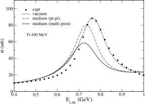
Figure 3: The $\pi\pi$ cross-section as a function of centre of mass energy. The dotted line indicates the cross-section obtained using eq. (3.30) which agrees well with the experimental values (eq. (3.27)) shown by filled squares. The dashed and solid lines depict the in-medium cross-section for $\pi\pi$ and $\pi h(h=\pi,\omega,h_{1},a_{1})$ loops respectively in the $\rho$ self-energy evaluated at $T$=160 MeV.

The strong interaction dynamics of the pions enters the collision integrals through the cross-section. In Fig. 3 we show the $\pi\pi$ cross-section as a function of the centre of mass energy of scattering. The different curves are explained below. The filled squares referred to as experiment is a widely used resonance saturation parametrization Bertsch1 ; Prakash of isoscalar and isovector phase shifts obtained from various empirical data involving the $\pi\pi$ system. The isospin averaged differential cross-section is given by

$$\frac{d\sigma(s)}{d\Omega}=\frac{4}{q_{cm}^{2}}\left[\frac{1}{9}\sin^{2}\delta^{0}_{0}+\frac{5}{9}\sin^{2}\delta^{2}_{0}+\frac{1}{3}\cdot 9\sin^{2}\delta_{1}^{1}\cos^{2}\theta\right]$$ (3.27)

where

$$\delta^{0}_{0} = \frac{\pi}{2}+\arctan\left(\frac{E-m_{\sigma}}{\Gamma_{\sigma}/2}\right)$$

$$\delta_{1}^{1} = \frac{\pi}{2}+\arctan\left(\frac{E-m_{\rho}}{\Gamma_{\rho}/2}\right)$$

$$\delta^{2}_{0} = -0.12p/m_{\pi}~{}.$$ (3.28)

The widths are given by $\Gamma_{\sigma}=2.06p$ and $\Gamma_{\rho}=0.095p\left(\frac{p/m_{\pi}}{1+(p/m_{\rho})^{2}}\right)^{2}$ with $m_{\sigma}=5.8m_{\pi}$ and $m_{\rho}=5.53m_{\pi}$ .

To get a handle on the dynamics we now evaluate the $\pi\pi$ cross-section involving $\rho$ and $\sigma$ meson exchange processes using the interaction Lagrangian

$${\cal L}=g_{\rho}\vec{\rho}^{\mu}\cdot\vec{\pi}\times\partial_{\mu}\vec{\pi}+\frac{1}{2}g_{\sigma}m_{\sigma}\vec{\pi}\cdot\vec{\pi}\sigma$$ (3.29)

where $g_{\rho}=6.05$ and $g_{\sigma}=2.5$. In the matrix elements corresponding to $s$-channel $\rho$ and $\sigma$ exchange diagrams which appear for total isospin $I=1$ and 0 respectively, we introduce a decay width in the corresponding propagator. We get Sukanya1 ,

$${\cal M}_{I=0} = g_{\sigma}^{2}m_{\sigma}^{2}\left[\frac{3}{s-m_{\sigma}^{2}+im_{\sigma}\Gamma_{\sigma}}+\frac{1}{t-m_{\sigma}^{2}}+\frac{1}{u-m_{\sigma}^{2}}\right]+2g_{\rho}^{2}\left[\frac{s-u}{t-m_{\rho}^{2}}+\frac{s-t}{u-m_{\rho}^{2}}\right]$$

$${\cal M}_{I=1} = g_{\sigma}^{2}m_{\sigma}^{2}\left[\frac{1}{t-m_{\sigma}^{2}}-\frac{1}{u-m_{\sigma}^{2}}\right]+g_{\rho}^{2}\left[\frac{2(t-u)}{s-m_{\rho}^{2}+im_{\rho}\Gamma_{\rho}}+\frac{t-s}{u-m_{\rho}^{2}}-\frac{u-s}{t-m_{\rho}^{2}}\right]$$

$${\cal M}_{I=2} = g_{\sigma}^{2}m_{\sigma}^{2}\left[\frac{1}{t-m_{\sigma}^{2}}+\frac{1}{u-m_{\sigma}^{2}}\right]+g_{\rho}^{2}\left[\frac{u-s}{t-m_{\rho}^{2}}+\frac{t-s}{u-m_{\rho}^{2}}\right]~{}.$$ (3.30)

The differential cross-section is then obtained from $\frac{d\sigma}{d\Omega}=\overline{|{\cal M}|^{2}}/64\pi^{2}s$ where the isospin averaged amplitude is given by $\overline{|{\cal M}|^{2}}=\frac{1}{9}\sum(2I+1)\overline{|{\cal M}_{I}|^{2}}$.

The integrated cross-section, after ignoring the $I=2$ contribution is shown by the dotted line (indicated by ’vacuum’) in Fig. 3 and is seen to agree reasonably well with the experimental cross-section up to a centre of mass energy of about 1 GeV beyond which the theoretical estimate gives higher values. We hence use the experimental cross-section beyond this energy.

After this normalisation to data, we now turn to the in-medium cross-section by introducing the effective propagator for the $\rho$ in the above expressions for the matrix elements. This is obtained in terms of the self-energy by solving the Dyson equation and is given by

$$D_{\mu\nu}=D^{(0)}_{\mu\nu}+D^{(0)}_{\mu\sigma}\Pi^{\sigma\lambda}D_{\lambda\nu}$$ (3.31)

where $D^{(0)}_{\mu\nu}$ is the vacuum propagator for the $\rho$ meson and $\Pi^{\sigma\lambda}$ is the self energy function obtained from one-loop diagrams shown in Fig. 4. The standard procedure Bellac to solve this equation in the medium is to decompose the self-energy into transverse and longitudinal components. For the case at hand the difference between these components is found to be small and is hence ignored. We work with the polarization averaged self-energy function defined as

$$\Pi=\frac{1}{3}(2\Pi^{T}+q^{2}\Pi^{L})$$ (3.32)

where

$$\Pi^{T}=-\frac{1}{2}(\Pi_{\mu}^{\mu}+\frac{q^{2}}{\bar{q}^{2}}\Pi_{00}),~{}~{}~{}~{}\Pi^{L}=\frac{1}{\bar{q}^{2}}\Pi_{00},~{}~{}~{}\Pi_{00}\equiv u^{\mu}u^{\nu}\Pi_{{\mu\nu}}~{}.$$ (3.33)

The in-medium propagator is then written as

$$D_{\mu\nu}(q_{0},\vec{q})=\frac{-g_{\mu\nu}+q_{\mu}q_{\nu}/q^{2}}{q^{2}-m_{\rho}^{2}-{\rm Re}\Pi(q_{0},\vec{q})+i{\rm Im}\Pi(q_{0},\vec{q})}~{}.$$ (3.34)

The scattering, decay and regeneration processes which cause a gain or loss of $\rho$ mesons in the medium are responsible for the imaginary part of its self-energy. The real part on the other hand modifies the position of the pole of the spectral function.

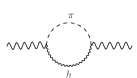
Figure 4: $\pi h$ self-energy diagrams where $h$ stands for $\pi,\omega,h_{1},a_{1}$ mesons.

As discussed in Sec. IIA, in the real-time formulation of thermal field theory the self-energy assumes a 2$\times$2 matrix structure of which the 11-component is given by

$$\Pi_{{\mu\nu}}^{11}(q)=i\int\frac{d^{4}k}{(2\pi)^{4}}N_{{\mu\nu}}(q,k)D_{\pi}^{11}(k)D_{h}^{11}(q-k)$$ (3.35)

where $D^{11}$ is the 11-component of the scalar propagator given by $D^{11}(k)=\Delta(k)+2\pi if^{(0)}(k)\delta(k^{2}-m^{2})$. It turns out that the self-energy function mentioned above can be obtained in terms of the 11-component through the relations Bellac ; Mallik_RT

$${\rm Re}\,\Pi_{{\mu\nu}} = {\rm Re}\,\Pi_{{\mu\nu}}^{11}$$

$${\rm Im}\Pi_{{\mu\nu}} = \epsilon(q_{0})\tanh(\beta q_{0}/2){\rm Im}\,\Pi_{{\mu\nu}}^{11}~{}.$$ (3.36)

Tensor structures associated with the two vertices and the vector propagator are included in $N_{{\mu\nu}}$ and are available in Ghosh1 where the interactions were taken from chiral perturbation theory. It is easy to perform the integral over $k_{0}$ using suitable contours to obtain

$${\Pi}^{{\mu\nu}}(q_{0},\boldsymbol{q}) = \int\frac{d^{3}k}{(2\pi)^{3}}\frac{1}{4\omega_{\pi}\omega_{h}}\left[\frac{(1+f^{(0)}(\omega_{\pi}))N^{{\mu\nu}}_{1}+f^{(0)}(\omega_{h})N^{{\mu\nu}}_{3}}{q_{0}-\omega_{\pi}-\omega_{h}+i\eta\epsilon(q_{0})}+\frac{-f^{(0)}(\omega_{\pi})N^{{\mu\nu}}_{1}+f^{(0)}(\omega_{h})N^{{\mu\nu}}_{4}}{q_{0}-\omega_{\pi}+\omega_{h}+i\eta\epsilon(q_{0})}\right.$$ (3.37)

$$+\left.\frac{f^{(0)}(\omega_{\pi})N^{{\mu\nu}}_{2}-f^{(0)}(\omega_{h})N^{{\mu\nu}}_{3}}{q_{0}+\omega_{\pi}-\omega_{h}+i\eta\epsilon(q_{0})}+\frac{-f^{(0)}(\omega_{\pi})N^{{\mu\nu}}_{2}-(1+f^{(0)}(\omega_{h}))N^{{\mu\nu}}_{4}}{q_{0}+\omega_{\pi}+\omega_{h}+i\eta\epsilon(q_{0})}\right]$$

where $f^{(0)}(\omega)=\frac{1}{e^{(\omega-\mu_{\pi})/T}-1}$ is the Bose distribution function with arguments $\omega_{\pi}=\sqrt{\boldsymbol{k}^{2}+m_{\pi}^{2}}$ and $\omega_{h}=\sqrt{(\boldsymbol{q}-\boldsymbol{k})^{2}+m_{h}^{2}}$. Note that this expression is a generalized form for the in-medium self-energy obtained by Weldon Weldon . The subscript $i(=1,..4)$ on $N^{{\mu\nu}}$ in (3.37) correspond to its values for $k_{0}=\omega_{\pi},-\omega_{\pi},q_{0}-\omega_{h},q_{0}+\omega_{h}$ respectively. It is easy to read off the real and imaginary parts from (3.37). The angular integration can be carried out using the $\delta$-functions in each of the four terms in the imaginary part which define the kinematically allowed regions in $q_{0}$ and $\boldsymbol{q}$ where scattering, decay and regeneration processes occur in the medium leading to the loss or gain of $\rho$ mesons Ghosh1 . The vector mesons $\omega$, $h_{1}$ and $a_{1}$ which appear in the loop have negative $G$-parity and have substantial $3\pi$ and $\rho\pi$ decay widths PDG . The (polarization averaged) self-energies containing these unstable particles in the loop graphs have thus been folded with their spectral functions,

$$\Pi(q,m_{h})=\frac{1}{N_{h}}\int^{(m_{h}+2\Gamma_{h})^{2}}_{(m_{h}-2\Gamma_{h})^{2}}dM^{2}\frac{1}{\pi}{\rm Im}\left[\frac{1}{M^{2}-m_{h}^{2}+iM\Gamma_{h}(M)}\right]\Pi(q,M)$$ (3.38)

with $N_{h}=\displaystyle\int^{(m_{h}+2\Gamma_{h})^{2}}_{(m_{h}-2\Gamma_{h})^{2}}dM^{2}\frac{1}{\pi}{\rm Im}\left[\frac{1}{M^{2}-m_{h}^{2}+iM\Gamma_{h}(M)}\right]$. The contributions from the loops with heavy mesons may then be considered as a multi-pion contribution to the $\rho$ self-energy.

The in-medium cross-section is now obtained by using the full $\rho$-propagator (3.34) in place of the usual vacuum propagator $D_{\mu\nu}^{(0)}$ in the scattering amplitudes. The long dashed line in Fig. 3 shows a suppression of the peak when only the $\pi\pi$ loop is considered. This effect is magnified when the $\pi h$ loops (solid line indicated by multi-pion) are taken into account and is also accompanied by a small shift in the peak position. Extension to the case of finite baryon density can be done using the spectral function computed in Ghosh2 where an extensive list of baryon (and anti-baryon) loops are considered along with the mesons. A similar modification of the $\pi\pi$ cross-section for a hot and dense system was seen also in Bertsch2 .

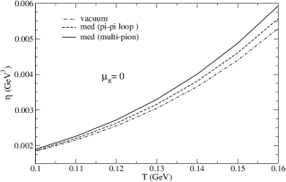
Figure 5: The shear viscosity as a function of temperature in the Chapman-Enskog approximation. The dash-dotted line indicates use of the vacuum cross-section and the dashed and solid lines correspond to in-medium cross-section for the $\pi\pi$ and multi-pion cases respectively.

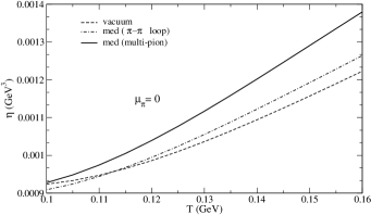
Figure 6: The shear viscosity as a function of temperature in the relaxation time approximation. The dash-dotted and solid lines correspond to the use of in-medium cross-sections in eq. (2.83) for $\pi\pi$ and multi-pion loops respectively. The dashed line represents the vacuum case.

We plot $\eta$ versus $T$ in Fig. 5 obtained in the Chapman-Enskog approximation showing the effect of the in-medium $\rho$ propagation in the pion gas Sukanya1 . We observe $\sim 10\%$ change at $T=150$ MeV due to medium effects compared to the vacuum when all the loops in the $\rho$ self-energy are considered. The effect reduces with temperature to less than $5\%$ at 100 MeV.

We noted in Sec. II that the lowest order result for $\eta$ in the response theory framework coincides with that obtained in the relaxation time approximation which is in fact the simplest way to linearize the transport equation. Here one assumes that $f(x,p)$ goes over to the equilibrium distribution $f^{(0)}(x,p)$ as a result of collisions and this takes place over a relaxation time $\tau(p)$ which is the inverse of the collision frequency defined in (2.83). The right hand side of eq. (3.1) is then given by $-E_{p}[f(x,p)-f^{(0)}(x,p)]/\tau(p)$ which subsequently leads to the expressions (2.81) and (2.82) for the shear and bulk viscosities Gavin . In Fig. 6 we show the temperature dependence of $\eta$ in the relaxation time approximation. The values in this case are lower than that obtained in the Chapman-Enskog method though the effect of the medium is larger. In addition to the fact that the expressions for the viscosities are quite different in two approaches, the difference in the numerical values obtained in the two cases also depends significantly on the energy dependence of the $\pi\pi$ cross-section Wiranata .

Figure 7: The bulk viscosity as a function of temperature for a chemically frozen pion gas. The dashed and solid lines correspond to the use of in-medium cross-sections in eq. (2.83) for $\pi\pi$ and multi-pion loops respectively. The dotted line represents the vacuum case.

In Fig. 7 we show the numerical results for the bulk viscosity of a pion gas as function of $T$. It is seen from an analysis of the left hand side of the transport equation that while the shear viscosity depends on elastic processes, bulk viscosity is sensitive to number changing processes. However in heavy ion collision experiments matter is known to undergo early chemical freeze-out. Number changing (inelastic) processes having much larger relaxation times go out of equilibrium at this point and a temperature dependent chemical potential results for each species so as to conserve the number corresponding to the measured particle ratios. We hence use a temperature dependent pion chemical potential taken from Hirano in this case. It is interesting to observe that $\zeta$ decreases with $T$ in contrast to $\eta$ which increases. The trend followed by $\zeta$ is similar to the findings of Moore . Additional discussions concerning the temperature dependence of viscosities for a chemically frozen pion gas are available in Sukanya2 .

IV Summary and Conclusion

To summarize, we have calculated the shear viscosity coefficient of a pion gas in the real time version of thermal field theory. It is simpler to the imaginary version in that we do not have to continue to imaginary time at any stage of the calculation. As an element in the theory of linear response, a transport coefficient is defined in terms of a retarded thermal two-point function of the components of the energy-momentum tensor. We derive Källen-Lehmann representation for any (bosonic) two-point function of both time-ordered and retarded types to get the relation between them. Once this relation is obtained, we can calculate the retarded function in the Feynman-Dyson framework of the perturbation theory.

Clearly the method is not restricted to transport coefficients. Any linear response leads to a retarded two-point function, which can be calculated in this way. Also quadratic response formulae have been derived in the real time formulation Carrington .

We have also evaluated the viscous coefficients in the kinetic theory approach to leading order in the Chapman-Enskog expansion. Here we have incorporated an in-medium $\pi\pi$ cross-section and found a significant effect in the temperature dependence of the shear viscosity.

The viscous coefficients and their temperature dependence could affect the quantitative estimates of signals of heavy ion collisions particularly where hydrodynamic simulations are involved. For example, it has been argued in Dusling that corrections to the freeze-out distribution due to bulk viscosity can be significant. As a result the hydrodynamic description of the $p_{T}$ spectra and elliptic flow of hadrons could be improved by including a realistic temperature dependence of the viscous coefficients. Such an evaluation essentially requires the consideration of a multi-component gas preferably containing nucleonic degrees of freedom so that extensions to finite baryon chemical potential can be made. Work in this direction is in progress.

References

- (1) P. Kovtun, D. T. Son and A. O. Starinets, Phys. Rev. Lett. 94, 111601 (2005).
- (2) L. P. Csernai, J. I. Kapusta and L. D. McLerran, Phys. Rev. Lett. 97, 152303 (2006).
- (3) H. B. Meyer, Eur. Phys. J. A 47 (2011) 86
- (4) N. Demir and S. A. Bass, Phys. Rev. Lett. 102 (2009) 172302
- (5) T. Matsubara, Prog. Theor. Phys. 14, 351 (1955)
- (6) R. Mills, Propagators for Many Particle Systems, Gordon and Breach, New York, 1969
- (7) H. Matsumoto, Y. Nakano and H. Umezawa, J. Math. Phys. 25, 3076 (1984)
- (8) A.J. Niemi and G.W. Semenoff, Ann. Phys. 152, 105 (1984).
- (9) R.L. Kobes and G.W. Semenoff, Nucl. Phys. 260, 714 (1985)
- (10) A. Hosoya, M. Sakagami and M. Takao, Ann. Phys. 154, 229 (1982).
- (11) R. Lang, N. Kaiser and W. Weise, hep-ph, 1205.6648v1
- (12) S. Jeon, Phys. Rev. 47, 4586 (1993)
- (13) G. Källen, Helv. Phys. Acra, 25, 417 (1952)
- (14) H. Lehmann, Nuovo Cimento, 11, 342 (1954)
- (15) A.L. Fetter and J.D. Walecka, Quantum theory of many-particle dystems, Dover Publications, New York, 2003
- (16) S. Mallik and S. Sarkar, Eur. Phys. J. C 61, 489 (2009).
- (17) S. Weinberg, Physica A 96 (1979) 327.
- (18) J. Gasser and H. Leutwyler, Annals Phys. 158, 142 (1984).
- (19) A. Dobado and S. N. Santalla, Phys. Rev. D 65, 096011 (2002).
- (20) J. W. Chen, Y. H. Li, Y. F. Liu and E. Nakano, Phys. Rev. D 76, 114011 (2007)
- (21) A. Dobado and F. J. Llanes-Estrada, Phys. Rev. D 69, 116004 (2004).
- (22) K. Itakura, O. Morimatsu and H. Otomo, Phys. Rev. D 77, 014014 (2008).
- (23) M. Prakash, M. Prakash, R. Venugopalan and G. Welke, Phys. Rept. 227 (1993) 321.
- (24) D. Davesne, Phys. Rev. C 53, 3069 (1996).
- (25) S. Mitra, S. Ghosh and S. Sarkar, Phys. Rev. C 85 (2012) 064917
- (26) R. Kubo, J. Phys. Soc. Japan, 12, 570 (1957)
- (27) P.C. Martin and J. Schwinger, Phys. Rev. 115, 1342 (1959)
- (28) D.N. Zubarev, Nonequilibrium Statistical Thermodynamics, Plenum, New York, 1974.
- (29) M. Gell-Mann and M. L. Golberger, Phys. Rev. D91 398 (1953)
- (30) J.L. Goity and H. Leutwyler, Phys. Lett. b 228(4), 517 (1989)
- (31) S. Mitra and S. Sarkar, Phys. Rev. D 87 (2013) 094206
- (32) P. Chakraborty and J. I. Kapusta, Phys. Rev. C 83 (2011) 014906.
- (33) W. A. Van Leeuwen, P. H. Polak and S. R. De Groot, Physica 66, 455 (1973).
- (34) G. Bertsch, M. Gong, L. D. McLerran, P. V. Ruuskanen and E. Sarkkinen, Phys. Rev. D 37 (1988) 1202.
- (35) M. Le Bellac, Thermal Field Theory (Cambridge University Press, Cambridge, 1996).
- (36) S. Sarkar, B. K. Patra, V. J. Menon and S. Mallik, Indian J. Phys. 76A (2002) 385
- (37) S. Ghosh, S. Sarkar and S. Mallik, Eur. Phys. J. C 70, 251 (2010).
- (38) H. A. Weldon, Phys. Rev. D 28 (1983) 2007.
- (39) K. Nakamura et al. [Particle Data Group], J. Phys. G 37 (2010) 075021.
- (40) S. Ghosh and S. Sarkar, Nucl. Phys. A 870-871, 94 (2011)
- (41) H. W. Barz, H. Schulz, G. Bertsch and P. Danielewicz, Phys. Lett. B 275 (1992) 19.
- (42) S. Gavin, Nucl. Phys. A 435 (1985) 826.
- (43) A. Wiranata and M. Prakash, Phys. Rev. C 85 (2012) 054908
- (44) T. Hirano and K. Tsuda, Phys. Rev. C 66 (2002) 054905
- (45) E. Lu and G. D. Moore, Phys. Rev. C 83 (2011) 044901
- (46) M. E. Carrington, H. Defu and R. Kobes, Phys. Rev. D64, 025001 (2001)
- (47) K. Dusling and T. Schafer, Phys. Rev. C 85 (2012) 044909