Constraints on Hyperluminous QSO Lifetimes via Fluorescent Ly$\alpha$ Emitters at $Z\simeq 2.7$

Abstract

We present observations of a population of Ly$\alpha$ emitters (LAEs) exhibiting fluorescent emission via the reprocessing of ionizing radiation from nearby hyperluminous QSOs. These LAEs are part of a survey at redshifts $2.5<z<2.9$ combining narrow-band photometric selection and spectroscopic follow-up to characterize the emission mechanisms, physical properties, and three-dimensional locations of the emitters with respect to their nearby hyperluminous QSOs. These data allow us to probe the radiation field, and thus the radiative history, of the QSOs, and we determine that most of the 8 QSOs in our sample have been active and of comparable luminosity for a time 1 Myr $\lesssim t_{\textrm{\scriptsize{Q}}}\lesssim 20$ Myr. Furthermore, we find that the ionizing QSO emission must have an opening angle $\theta\sim 30\arcdeg$ or larger relative to the line of sight.

1. Introduction

The extreme luminosities of QSOs make them effective tracers of black hole growth over most of the Universe’s history ($0<z\lesssim 7$) and likewise illuminate the evolution of galaxies and large-scale structure over these cosmological epochs and volumes. In particular, the mass of supermassive black holes is tightly correlated with properties of their host galaxies (e.g. Magorrian et al. 1998; Gebhardt et al. 2000; Ferrarese & Merritt 2000), while QSO clustering properties are well-matched to the expected distribution of dark matter in and out of halos (e.g. Seljak 2000; Berlind & Weinberg 2002; Zehavi et al. 2004) according to the cosmological standard model.

However, the manner in which QSOs populate and interact with galaxies and dark-matter halos is obscured by the unknown timescales and geometries over which black holes accrete mass and produce substantial radiation. Specifically, the fraction of black holes that can be observed as QSOs depends sensitively on the length of their active phases and whether their emission is isotropic or confined to a narrow solid angle. A short QSO lifetime ($t_{\textrm{\scriptsize{Q}}}$) and/or a small opening angle ($\theta_{\textrm{\scriptsize{Q}}}$) would indicate that observed QSOs comprise a small fraction of the total population of black holes (and therefore galaxies and dark-matter halos) that will pass through a QSO phase. Furthermore, both the comparison of $t_{\textrm{\scriptsize{Q}}}$ to a typical star-formation timescale $t_{\textrm{\scriptsize{SF}}}\sim 100$ Myr and the value of $\theta_{\textrm{\scriptsize{Q}}}$ have deep implications for the mechanisms by which the QSO couples to the ISM in galaxies and produces feedback.

Current estimates of $t_{\textrm{\scriptsize{Q}}}$ utilize numerous methods, many of which are described in detail in a review by Martini (2004), and in general allow for QSO lifetimes in the range $10^{6}$ yr $<t_{\textrm{\scriptsize{Q}}}<10^{8}$ yr. In the last decade, measurements of the QSO luminosity function and clustering have provided particularly powerful constraints on a globally-averaged $t_{\textrm{\scriptsize{Q}}}$ (e.g. Kelly et al. 2010), but they also rely on the poorly-constrained black hole mass function or assume that the most luminous QSOs populate the most massive halos, contrary to some observations and physically-motivated models (e.g. Trainor & Steidel 2012; Adelberger & Steidel 2005; Conroy & White 2013). These global measures of $t_{\textrm{\scriptsize{Q}}}$ are also degenerate between single-phase QSO accretion (in which the bulk of activity occurs in a single event) and multi-burst models (in which the same total time in a QSO phase is distributed over many short accretion events).

More direct measurements of $t_{\textrm{\scriptsize{Q}}}$ may be obtained from the effect of QSO radiation on their local enviroments. Measures of the transverse proximity effect use the volumes (and associated light-travel times) over which bright QSOs ionize their nearby gas and have yielded estimates or lower limits in the range $t_{\textrm{\scriptsize{Q}}}\sim 16-40$ Myr by tracing He II (e.g. Jakobsen et al. 2003; Worseck et al. 2007) and metal-line (Gonçalves et al., 2008) absorption systems.

The detection of fluorescent Ly$\alpha$ emission provides another direct measurement of $t_{\textrm{\scriptsize{Q}}}$. Fluorescent Ly$\alpha$ arises from the reprocessing of ionizing photons (either from the metagalactic UV background or a local QSO) at the surfaces of dense, neutral clouds of H I. This effect has been modeled with increasing complexity over the last few decades (Hogan & Weymann, 1987; Gould & Weinberg, 1996; Cantalupo et al., 2005; Kollmeier et al., 2010) and has now been observed around bright QSOs (Adelberger et al. 2006; Cantalupo et al. 2007, 2012; Trainor et al. 2013, in prep.). These detections have verified the feasibility of identifying fluorescent emission from the intergalactic medium (IGM) and suggested a wide opening angle $\theta_{\textrm{\scriptsize{Q}}}$ of QSO emission (but see also Hennawi & Prochaska 2013). They are consistent with other constraints on $t_{\textrm{\scriptsize{Q}}}$, but have been limited by small sample sizes and/or a lack of the 3D spatial information necessary to probe the spatial variation of the QSO radiation field in detail.

This paper presents results from a large survey of Ly$\alpha$ emitters (LAEs) in fields surrounding hyperluminous ($L_{\textrm{\scriptsize{UV}}}\sim 10^{14}$ L${}_{\textrm{\scriptsize{$\sun$}}}$) QSOs at redshifts $2.5<z<2.9$. The full results of this survey, including a detailed analysis of the Ly$\alpha$ emission mechanisms and physical properties of the LAEs, will be presented in Trainor et al. (2013, in prep.; hereafter Paper II). This paper focuses on the implications of these data for $t_{\textrm{\scriptsize{Q}}}$ and $\theta_{\textrm{\scriptsize{Q}}}$. Observations and the data are briefly discussed in §2; identification of fluorescent sources is discussed in §3.1; constraints on $t_{\textrm{\scriptsize{Q}}}$ and $\theta_{\textrm{\scriptsize{Q}}}$ appear in §3.2$-$§3.5; and conclusions are given in §4. A standard cosmology with $H_{0}=70$ km s^-1 and $\{\Omega_{\textrm{\scriptsize{m}}},\Omega_{\Lambda}\}=\{0.3,0.7\}$ is assumed throughout, and distances are given in physical units (e.g. pMpc).

2. Observations

We conducted deep imaging in each survey field using custom narrow-band filters and corresponding broad-band filters sampling the continuum near Ly$\alpha$ with Keck 1/LRIS-B over several years; these data are described in Paper II. All 8 fields are part of the Keck Baryonic Structure Survey (KBSS; Rudie et al. 2012; Steidel et al. 2013, in prep.)

We used 1 of 4 narrow-band filters to image each of the 8 QSO fields (centered on or near the QSO); a brief description of the fields and corresponding filters is given in Table 1. Each filter has a FWHM $\sim 80$Å and a central wavelength tuned to Ly$\alpha$ at the redshift of one or more of the hyperluminous QSOs. The QSOs span a redshift range $2.573\leq z\leq 2.843$, and the filter width corresponds to $\Delta z\approx 0.066$ or $\Delta v\approx 5400$ km s^-1 at their median redshift. The narrow-band images have total integration times of 5-7 hours and reach a depth for point sources of $m_{\textrm{\scriptsize{NB}}}(3\sigma)\sim 26.7$; the continuum images are typically deeper by $\sim 1.5$ mag.

Object identification and narrow-band and continuum magnitude measurements were performed with SExtractor. The success rate of our initial follow-up spectroscopy dropped sharply above $m_{\textrm{\scriptsize{NB}}}=26.5$, so our LAEs are selected to have $20<m_{\textrm{\scriptsize{NB}}}<26.5$ and $m_{\textrm{\scriptsize{cont}}}-m_{\textrm{\scriptsize{NB}}}>0.6$ (corresponding to a rest-frame equivalent width in Ly$\alpha$ $W_{0}\gtrsim 20$Å). These criteria define a set of 841 LAEs. The LAEs range from unresolved/compact to extremely extended (FWHM $\gtrsim 10\arcsec$) sources. The extended objects require large photometric apertures that may enclose unassociated continuum sources; in order to avoid the complication of determining the true continuum counterparts of these sources, LAEs with FWHM $>3\arcsec$ were removed from our sample for this analysis, leaving a final photometric sample of 816 LAEs.

Spectra were obtained with Keck 1/LRIS-B in the multislit mode using the 600/4000 grism; the spectral resolution near Ly$\alpha$ for these spectra is $R\sim 1100$. Redshifts were measured via an automated algorithm described in Paper II; the detected Ly$\alpha$ lines have a minimum SNR $\sim$ 3.5 and a median SNR $\sim$ 15. Detected lines were required to lie at a wavelength where the transmission exceeds 10% for the narrow-band filter used to select their associated candidates (typically a $\sim$110Å range), but no other prior was used to constrain the automatic line detection. Redshifts were measured for 260 of the LAEs meeting our final photometric criteria; these comprise the spectroscopic sample used in this paper. QSO redshifts were determined as described in Trainor & Steidel (2012) and have estimated uncertainties $\sigma_{\textrm{\scriptsize{z,QSO}}}\approx 270$ km s^-1.

3. Results

3.1. Detection of Fluorescent Emission

Ly$\alpha$ emission is subject to complex radiative-transfer effects and is ubiquitous in star-forming galaxies, so accurate discrimination between fluorescence and other Ly$\alpha$ emission mechanisms is key to its use as a QSO probe (see Cantalupo et al. 2005; Kollmeier et al. 2010). A powerful tool in this regard is the rest-frame equivalent width of Ly$\alpha$ ($W_{0}$), which has a natural maximum in star-forming sources because the same massive stars produce the UV continuum and the ionizing photons that are reprocessed as Ly$\alpha$ emission. Empirically, UV-continuum-selected galaxies at $2\lesssim z\lesssim 3$ almost never exhibit $W_{0}>100$Å (Kornei et al., 2010), which is also the maximum value expected for continuous star-formation lasting $\sim 10^{8}$ yr or longer (Steidel et al., 2011). This threshold may demarcate the realm of fluorescence from that of typical star-forming galaxies. Furthermore, models of star-formation in the extreme limits of metallicity and short bursts predict a stringent limit of $W_{0}<240$ Å (see Schaerer 2002 and discussion in Cantalupo et al. 2012) for even the most atypical star-forming galaxies.

The distribution of $W_{0}$ and $m_{\textrm{\scriptsize{NB}}}$ for the LAEs are displayed in Fig. 1. Observed-frame equivalent widths ($W$) were measured from the narrow-band color excess while accounting for the presence of Ly$\alpha$ within the continuum filter bandpass; details of this procedure are given in Paper II. $W_{0}$ is estimated from $W$ by $W_{0}=W/(1+z_{\textrm{\scriptsize{QSO}}})$, where $z_{\textrm{\scriptsize{QSO}}}$ is the redshift of the associated hyperluminous QSO.

Fig. 1 demonstrates that many of our LAEs exceed both the model and empirical thresholds for the maximum $W_{0}$ consistent with pure star formation: of the 816 LAEs, 116 exceed $W_{0}>100$Å and 32 exceed $W_{0}>240$Å. We consider these high-$W_{0}$ sources as excellent candidates to be fluorescence-dominated, with minimal stellar contribution to their Ly$\alpha$ flux.

3.2. Time delay of fluorescent emission

The presence of a fluorescent emitter indicates that its local volume element was illuminated by ionizing QSO radiation at the lookback time $t_{\textrm{\scriptsize{Ly$\alpha$}}}$ when the observed Ly$\alpha$ photon was emitted. Depending on whether the fluorescent source lies in the foreground or background of the QSO, $t_{\textrm{\scriptsize{Ly$\alpha$}}}$ may be greater or less than $t_{\textrm{\scriptsize{QSO}}}$, the lookback time to the QSO itself.

However, this fluorescent Ly$\alpha$ photon was generated by the reprocessing of an ionizing QSO photon emitted a time $t_{\textrm{\scriptsize{lt}}}$ before $t_{\textrm{\scriptsize{Ly$\alpha$}}}$, where $t_{\textrm{\scriptsize{lt}}}$ is the light-travel time from the QSO to the emitter. It is geometrically trivial to show that $t_{\textrm{\scriptsize{QSO}}}\leq t_{\textrm{\scriptsize{Ly$\alpha$}}}+t_{\textrm{\scriptsize{lt}}}$, and we can define the delay time for an emitter at a vector position ${\bf r}$:

$$t_{\textrm{\scriptsize{delay}}}({\bf r})=t_{\textrm{\scriptsize{Ly$\alpha$}}}({\bf r})+t_{\textrm{\scriptsize{lt}}}({\bf r})-t_{\textrm{\scriptsize{QSO}}}\,\,.$$ (1)

It can likewise be shown that the locus of points for which $t_{\textrm{\scriptsize{delay}}}$ is constant forms a paraboloid pointed toward the observer with the QSO at the focal point (see Fig. 2, top, for a pictorial representation at varying values of $t_{\textrm{\scriptsize{delay}}}$).

The significance of such a delay surface can be seen by considering a simple, step-function model of QSO emission in which the ionizing emission was zero a time $t_{\textrm{\scriptsize{Q}}}$ before we observe the QSO and has been constant since that time. Under such a model, the ionizing field is zero for $t_{\textrm{\scriptsize{delay}}}({\bf r})>t_{\textrm{\scriptsize{Q}}}$, and the spatial distribution of fluorescent emitters must be restricted to the interior of the paraboloid defined by $t_{\textrm{\scriptsize{delay}}}({\bf r})=t_{\textrm{\scriptsize{Q}}}$.

Since the high-$W_{0}$ LAEs described in §3.1 are highly likely to be dominated by fluorescence, they represent the best tracers of the QSO ionizing field. Below, we use the distribution of these sources to set limits on $t_{\textrm{\scriptsize{Q}}}$.

3.3. Constraints on $t_{\textrm{\scriptsize{Q}}}$ from the redshift distribution

The geometry of our survey volume is such that we can probe long timescales $(10^{7}$ yr $\lesssim t_{\textrm{\scriptsize{Q}}}\lesssim 10^{8}$ yr$)$ via the line-of-sight distribution of sources (see red box in Fig. 2, top). The distribution of $W_{0}$ vs. $d_{\textrm{\scriptsize{z}}}$ for the 260 LAEs with measured redshifts is displayed in Fig. 2 (middle), where $d_{\textrm{\scriptsize{z}}}$ is the Hubble distance of each emitter from its associated hyperluminous QSO determined from the difference of emitter and QSO redshifts.

Due to the effects of redshifts errors and peculiar velocities among the LAEs and QSOs, our foreground/background discrimination breaks down at $\Delta v\approx 700$ km s^-1, corresponding to $d_{\textrm{\scriptsize{z}}}\lesssim 3$ pMpc and $t_{\textrm{\scriptsize{delay}}}\lesssim 20$ Myr; we are therefore unable to constrain $t_{\textrm{\scriptsize{Q}}}$ lower than 20 Myr based on the redshift distribution of sources. At $t_{\textrm{\scriptsize{delay}}}>20$ Myr, however, there is a significant paucity of high-$W_{0}$ sources: only four sources with $W_{0}>100$Å lie in this range, and there are none at $t_{\textrm{\scriptsize{delay}}}>33$ Myr. This suggests $t_{\textrm{\scriptsize{Q}}}\lesssim 20$ Myr for these fields; we evaluate the significance of this result via numerical tests below.

The non-uniform redshift coverage of our QSO fields complicates the analysis of $d_{\textrm{\scriptsize{z}}}$; the observed redshift distribution is modulated by the narrow-band filter bandpass and the distribution of large-scale structure along the QSO line of sight. In addition, the QSO redshifts are not perfectly centered in their filter bandpasses, which contributes part of the observed asymmetry. Fortunately, the distribution of star-forming galaxies presumably represented by our $W_{0}<100$Å LAEs trace all of these effects, and we can use their redshift distribution to determine the expected distribution of emitters in the absence of fluorescence. We use the entire sample of emitters with spectroscopic redshifts and $W_{0}<100$Å for this comparison.

Firstly, we utilize the two-sample Kolmogorov-Smirnov (KS) test, a measure of the probability that two samples of observations are drawn from the same parent distribution. Evaluating the test on the distributions of $d_{\textrm{\scriptsize{z}}}(W_{0}>100$Å$)$ and $d_{\textrm{\scriptsize{z}}}(W_{0}\leq 100$Å$)$ yields a KS statistic $M_{\textrm{\scriptsize{KS}}}=0.234$, corresponding to $p<4\times 10^{-3}$. There are insufficient emitters with redshift measurements to perform the test on the higher-threshold ($W_{0}>240$Å) sample with significance.

A disadvantage of the two-sample KS test is that it is most sensitive to differences that occur near the center of two distributions, whereas we expect the strongest deviation in these distributions at large $d_{\textrm{\scriptsize{z}}}$, where no fluorescent emitters would appear if $t_{\textrm{\scriptsize{Q}}}\lesssim 20$ Myr. For this reason, we conducted a Monte-Carlo test in which subsamples of the $W_{0}<100$Å LAEs were randomly selected (with replacement), where each subsample has 67 objects, the number of $W_{0}>100$Å emitters with spectroscopic redshifts in our actual sample. For each subsample, the number of sources with $d_{\textrm{\scriptsize{z}}}>3$ pMpc (corresponding to $t_{\textrm{\scriptsize{delay}}}\gtrsim 20$ Myr) was counted.

As noted above, only four sources with $W_{0}>100$Å exceed $d_{\textrm{\scriptsize{z}}}=3$ pMpc. In $10^{5}$ simulated subsamples, 40 had three or fewer objects with $d_{\textrm{\scriptsize{z}}}>3$ pMpc, yielding a significance $p<4\times 10^{-4}$. We therefore conclude that the 7 QSOs with spectroscopic follow-up (ie. all except Q2343+12) are consistent with $t_{\textrm{\scriptsize{Q}}}\lesssim 20$ Myr (approximately the lowest it can be measured unambiguously from our redshift measurements).

3.4. Constraints on $t_{\textrm{\scriptsize{Q}}}$ from the projected distribution

While the redshift distribution is not sensitive for probing shorter QSO lifetimes, sufficiently small values of $t_{\textrm{\scriptsize{Q}}}$ will affect the projected distribution of sources in the survey volume. In particular, the constant-$t_{\textrm{\scriptsize{delay}}}$ paraboloids for $t_{\textrm{\scriptsize{delay}}}\lesssim 1$ Myr are well matched to the geometry of our survey volume (see curves on the left side of Fig. 2, top).

Fig. 3 shows the correspondence of these surfaces (shown for $10^{4}$ yr $\leq t_{\textrm{\scriptsize{delay}}}\leq 10^{6}$ yr) to the radial distribution of $W_{0}$ for the entire photometric sample (note that the survey geometry is not to scale, unlike in Fig. 2). As above, a QSO with $t_{\textrm{\scriptsize{Q}}}\leq t_{\textrm{\scriptsize{delay}}}$ will produce fluorescent emission only within the corresponding paraboloid. For $t_{\textrm{\scriptsize{Q}}}<0.3$ Myr, this would produce a maximum projected distance ($d_{\textrm{\scriptsize{$\theta$}}}$) at which a fluorescent emitter could appear in our survey volume. For $0.3$ Myr $\leq t_{\textrm{\scriptsize{Q}}}\leq 1$ Myr, the fractional volume of the survey within the time-delay surface decreases with increasing $d_{\textrm{\scriptsize{$\theta$}}}$, predicting that the probability of a given emitter exhibiting fluorescence will likewise decrease with $d_{\textrm{\scriptsize{$\theta$}}}$.

Notably, the projected distribution of LAEs is well-populated by objects with $W_{0}>100$Å and those with $W_{0}>240$Å out to the largest values of $d_{\textrm{\scriptsize{$\theta$}}}$ probed by our survey, thus firmly ruling out lifetimes $t_{\textrm{\scriptsize{Q}}}<0.3$ Myr. Furthermore, the radial distributions of sources with $W_{0}>100$Å and $W_{0}\leq 100$Å are entirely consistent when subjected to a two sample KS test ($M_{\textrm{\scriptsize{KS}}}=0.095$; $p<0.24$); the null result is similar using the $W_{0}=240$Å threshold. Given the large number of objects in our photometric sample ($N_{\textrm{\scriptsize{phot}}}=816$), these data provide strong evidence that $t_{\textrm{\scriptsize{Q}}}\gtrsim 1$ Myr for the QSOs in our sample.

3.5. Constraints on $\theta_{\textrm{\scriptsize{Q}}}$

For $\theta_{\textrm{\scriptsize{Q}}}\ll\pi/2$, a substantial fraction of the survey volume at large $d_{\textrm{\scriptsize{$\theta$}}}$ will be inaccessible to the ionizing emission of the QSO, which will affect the distribution of $d_{\textrm{\scriptsize{$\theta$}}}$ for fluorescent sources similarly to $t_{\textrm{\scriptsize{Q}}}\ll 1$ Myr. We can probe $\theta_{\textrm{\scriptsize{Q}}}$ in detail through the 2D spatial distribution of those high-$W_{0}$ LAEs with spectroscopic redshifts. It is easily seen in Fig. 3 (top) that the high-$W_{0}$ LAEs (red and orange points) extend to large projected radii at or near the QSO redshift, suggesting that ionizing emission is emanating from the QSO nearly perpindicularly to the line of sight (ie. with $\theta_{\textrm{\scriptsize{Q}}}\sim 90\deg$). In reality, redshift errors and peculiar velocities prohibit us from establishing the line-of-sight distance of an LAE from the QSO to be less than 3 pMpc (see §3.3), so these data (with a 2 pMpc projected range) provide the constraint $\theta_{\textrm{\scriptsize{Q}}}\gtrsim\arctan(2/3)\approx 30\deg$.

4. Conclusions

We have presented constraints on the lifetime and opening angle of ionizing QSO emission based on a large photometric/spectroscopic survey of LAEs in the regions around hyperluminous QSOs (described in detail in Paper II), finding 1 Myr $\lesssim t_{\textrm{\scriptsize{Q}}}\lesssim$ 20 Myr and $\theta_{\textrm{\scriptsize{Q}}}\gtrsim 30\arcdeg$.

These results are consistent with the most of the literature discussed in §1; in particular, our estimate of $t_{\textrm{\scriptsize{Q}}}$ falls at the short end of the broad range allowed by the measurements reviewed in Martini (2004) and is similar to the transverse proximity effect measurements of Gonçalves et al. (2008), which included a QSO of comparable luminosity to those in this sample. Perhaps most significantly, $t_{\textrm{\scriptsize{Q}}}$ measured here is short compared to the $e$-folding timescale of Salpeter (1964): $t_{\textrm{\scriptsize{Sal}}}=M_{\textrm{\scriptsize{BH}}}/\dot{M}_{\textrm{\scriptsize{BH}}}\approx 45$ Myr for a QSO with $L=L_{\textrm{\scriptsize{Edd}}}$ and a radiative efficiency $\epsilon=L/\dot{M}c^{2}=0.1$. Unless these QSOs have $L\gg L_{\textrm{\scriptsize{Edd}}}$ or are accreting with a low radiative efficiency (neither of which is expected for luminous QSOs), then these observed hyperluminous accretion events do not dominate the accretion history of their central black holes.

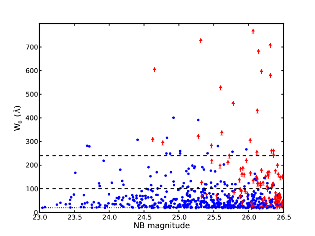
Figure 1.— The rest-frame equivalent width ($W_{0}$) of Ly$\alpha$ determined from the measured $m_{\textrm{\scriptsize{cont}}}-m_{\textrm{\scriptsize{NB}}}$ color for each LAE in our photometric sample. Objects detected in the continuum band are displayed as blue circles, while objects consistent with having no continuum flux (after subtracting the measured Ly$\alpha$ flux) are displayed as red arrows denoting 1$\sigma$ lower limits. Thresholds for the maximum value of $W_{0,Ly\alpha}$ consistent with typical and extremely brief star-formation are plotted as dashed lines at $W_{0}=100$Å and $W_{0}=240$Å, respectively (see §3.1 for details). The dotted line at $W_{0}=20$Å denotes the minimum Ly$\alpha$ equivalent width for a LAE.

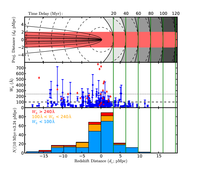
Figure 2.— Redshift constraints on QSO lifetimes. Top: Schematic representation of QSO light travel with observer lying to the left of the plot. Dashed circles represent the current position of photons emitted by the QSO 10 Myr, 20 Myr, … 60 Myr ago. Shaded parabolas on right side denote surfaces of constant $t_{\textrm{\scriptsize{delay}}}$. For the simple model of QSO emission discussed in §LABEL:subsec:qsos, sources may only exhibit fluorescent emission if they lie in the foreground of the surface for which $t_{\textrm{\scriptsize{delay}}}=t_{\textrm{\scriptsize{Q}}}$, where $t_{\textrm{\scriptsize{Q}}}$ is the QSO lifetime. The red region shows the geometry of this survey, for which surfaces of constant time delay are well-approximated by surfaces of constant redshift (green lines) for $t_{\textrm{\scriptsize{delay}}}\gtrsim 20$ Myr. The narrow parabolas on the left side are time-delay surfaces for $t_{\textrm{\scriptsize{delay}}}\leq$ 1 Myr, which are shown in more detail in Fig. 3. Middle: Ly$\alpha$ equivalent width ($W_{0}$) as a function of line-of-sight distance from the QSO for LAEs with measured redshifts. Red limits and blue points are plotted as in Fig. 1 with the addition of 1$\sigma$ error bars. Nearly all points with $W_{0}>100$Å lie in the foreground of the $t_{\textrm{\scriptsize{delay}}}=20$ Myr surface. Bottom: The redshift distribution of emitters in three bins of $W_{0}$, where $W_{0}$ is either the detected value or the 1$\sigma$ lower limit. The fraction of emitters with $W_{0}>100$Å drops sharply for $d_{\textrm{\scriptsize{z}}}>10$ Mlyr $\approx$ 3.24 pMpc.

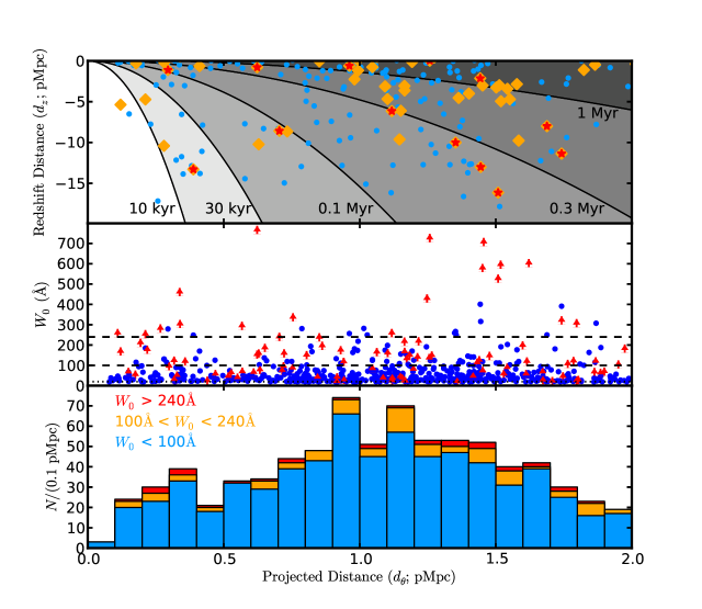
Figure 3.— Plane-of-sky constraints on QSO lifetimes. Top: Schematic representation of QSO region (as in Fig. 2, top), with observer lying to the bottom of the plot. Shaded parabolas denote surfaces of constant time delay ($10^{4}\leq t_{\textrm{\scriptsize{delay}}}\leq 10^{6}$ as noted on figure). For all lifetimes $t_{\textrm{\scriptsize{Q}}}\lesssim 1$ Myr, few or no fluorescent sources are predicted at large ($d_{\textrm{\scriptsize{$\theta$}}}\sim 2$ pMpc) separations from the QSO for our survey geometry. The 2D distribution of spectroscopic LAEs is shown for comparison as $W_{0}<100$Å (blue dots), $W_{0}>100$Å (orange diamonds), and $W_{0}>240$Å (red stars). Middle: Ly$\alpha$ equivalent width ($W_{0}$) as a function of projected distance from the QSO for photometrically-identified LAEs. Red limits and blue points are plotted as in Fig. 1. Sources with $W_{0}>100$Å are common out to the maximum projected distances probed by our survey volume, suggesting that the QSOs in our sample have lifetimes $t_{\textrm{\scriptsize{Q}}}\gtrsim 1$ Myr. Bottom: The projected distribution of emitters in three bins of $W_{0}$, where $W_{0}$ is either the detected value or the 1$\sigma$ lower limit. The fraction of emitters with $W_{0}>100$Å is fairly constant for $d_{\textrm{\scriptsize{$\theta$}}}<2$ pMpc.

Table 1Field Descriptions

QSO Field	$z_{\textrm{\scriptsize{Q}}}$	NB Filter	$N_{\textrm{\scriptsize{phot}}}$	$N_{\textrm{\scriptsize{spec}}}$	$N_{\textrm{\scriptsize{$W_{0}$$>$100\AA}}}$
Q0100+13 (PHL957)	$2.721\pm 0.001$	NB4535	79	20	9
HS0105+1619	$2.652\pm 0.001$	NB4430	109	23	6
Q0142$-$10 (UM673a)	$2.743\pm 0.001$	NB4535	58	25	11
Q1009+29 (CSO 38)	$2.652\pm 0.001$	NB4430	60	35	13
HS1442+2931	$2.660\pm 0.001$	NB4430	120	39	23
HS1549+1919	$2.843\pm 0.001$	NB4670	202	95	27
HS1700+6416	$2.751\pm 0.001$	NB4535	66	23	11
Q2343+12	$2.573\pm 0.001$	NB4325	122	0	16

References

- Adelberger & Steidel (2005) Adelberger, K. L., & Steidel, C. C. 2005, ApJ, 630, 50, 50
- Adelberger et al. (2006) Adelberger, K. L., Steidel, C. C., Kollmeier, J. A., & Reddy, N. A. 2006, ApJ, 637, 74, 74
- Berlind & Weinberg (2002) Berlind, A. A., & Weinberg, D. H. 2002, ApJ, 575, 587, 587
- Cantalupo et al. (2012) Cantalupo, S., Lilly, S. J., & Haehnelt, M. G. 2012, MNRAS, 425, 1992, 1992
- Cantalupo et al. (2007) Cantalupo, S., Lilly, S. J., & Porciani, C. 2007, ApJ, 657, 135, 135
- Cantalupo et al. (2005) Cantalupo, S., Porciani, C., Lilly, S. J., & Miniati, F. 2005, ApJ, 628, 61, 61
- Conroy & White (2013) Conroy, C., & White, M. 2013, ApJ, 762, 70, 70
- Ferrarese & Merritt (2000) Ferrarese, L., & Merritt, D. 2000, ApJ, 539, L9, L9
- Gebhardt et al. (2000) Gebhardt, K., Bender, R., Bower, G., et al. 2000, ApJ, 539, L13, L13
- Gonçalves et al. (2008) Gonçalves, T. S., Steidel, C. C., & Pettini, M. 2008, ApJ, 676, 816, 816
- Gould & Weinberg (1996) Gould, A., & Weinberg, D. H. 1996, ApJ, 468, 462, 462
- Hennawi & Prochaska (2013) Hennawi, J. F., & Prochaska, J. X. 2013, ApJ, 766, 58, 58
- Hogan & Weymann (1987) Hogan, C. J., & Weymann, R. J. 1987, MNRAS, 225, 1P, 1P
- Jakobsen et al. (2003) Jakobsen, P., Jansen, R. A., Wagner, S., & Reimers, D. 2003, A&A, 397, 891, 891
- Kelly et al. (2010) Kelly, B. C., Vestergaard, M., Fan, X., et al. 2010, ApJ, 719, 1315, 1315
- Kollmeier et al. (2010) Kollmeier, J. A., Zheng, Z., Davé, R., et al. 2010, ApJ, 708, 1048, 1048
- Kornei et al. (2010) Kornei, K. A., Shapley, A. E., Erb, D. K., et al. 2010, ApJ, 711, 693, 693
- Magorrian et al. (1998) Magorrian, J., Tremaine, S., Richstone, D., et al. 1998, AJ, 115, 2285, 2285
- Martini (2004) Martini, P. 2004, Coevolution of Black Holes and Galaxies, 169, 169
- Press & Schechter (1974) Press, W. H., & Schechter, P. 1974, ApJ, 187, 425, 425
- Rudie et al. (2012) Rudie, G. C., Steidel, C. C., Trainor, R. F., et al. 2012, ApJ, 750, 67, 67
- Salpeter (1964) Salpeter, E. E. 1964, ApJ, 140, 796, 796
- Schaerer (2002) Schaerer, D. 2002, A&A, 382, 28, 28
- Seljak (2000) Seljak, U. 2000, MNRAS, 318, 203, 203
- Steidel et al. (2011) Steidel, C. C., Bogosavljević, M., Shapley, A. E., et al. 2011, ApJ, 736, 160, 160
- Trainor & Steidel (2012) Trainor, R. F., & Steidel, C. C. 2012, ApJ, 752, 39, 39
- Worseck et al. (2007) Worseck, G., Fechner, C., Wisotzki, L., & Dall’Aglio, A. 2007, A&A, 473, 805, 805
- Zehavi et al. (2004) Zehavi, I., Weinberg, D. H., Zheng, Z., et al. 2004, ApJ, 608, 16, 16