Near-polytropic stellar simulations with a radiative surface

Abstract

Context. Studies of solar and stellar convection often employ simple polytropic setups using the diffusion approximation instead of solving the proper radiative transfer equation. This allows one to control separately the polytropic index of the hydrostatic reference solution, the temperature contrast between top and bottom, and the Rayleigh and Péclet numbers.

Aims. Here we extend such studies by including radiative transfer in the gray approximation using a Kramers-like opacity with freely adjustable coefficients. We study the properties of such models and compare them with results from the diffusion approximation.

Methods. We use the Pencil Code, which is a high-order finite difference code where radiation is treated using the method of long characteristics. The source function is given by the Planck function. The opacity is written as $\kappa=\kappa_{0}\rho^{a}T^{b}$, where $a=1$ in most cases, $b$ is varied from $-3.5$ to $+5$, and $\kappa_{0}$ is varied by four orders of magnitude. We adopt a perfect monatomic gas. We consider sets of one-dimensional models and perform a comparison with the diffusion approximation in one- and two-dimensional models.

Results. Except for the case where $b=5$, we find one-dimensional hydrostatic equilibria with a nearly polytropic stratification and a polytropic index close to $n=(3-b)/(1+a)$, covering both convectively stable ($n>3/2$) and unstable ($n<3/2$) cases. For $b=3$ and $a=-1$, the value of $n$ is undefined a priori and the actual value of $n$ depends then on the depth of the domain. For large values of $\kappa_{0}$, the thermal adjustment time becomes long, the Péclet and Rayleigh numbers become large, and the temperature contrast increases and is thus no longer an independent input parameter, unless the Stefan–Boltzmann constant is considered adjustable.

Conclusions. Proper radiative transfer with Kramers-like opacities provides a useful tool for studying stratified layers with a radiative surface in ways that are more physical than what is possible with polytropic models using the diffusion approximation.

1 Introduction

Convection in stars and accretion disks is a consequence of radiative cooling at the surface. Pioneering work by Nordlund (1982, 1985) has shown that realistic simulations of solar granulation can be performed with not too much extra effort and the required computing resources are comparable to the mandatory costs for solving the hydrodynamics part. Yet, many studies of hydrodynamic and hydromagnetic convection today ignore the effects of proper radiative transfer, sometimes even at the expense of using compute-intensive implicit solvers to cope with a computationally stiff problem in the upper layers where the radiative conductivity becomes large (e.g., Cattaneo et al., 1991; Gastine & Dintrans, 2008). Therefore, the main reason for ignoring radiation cannot be just the extra effort, but it is more likely a reduced flexibility in that one is confined to a single physical realization of a system and the difficulty in varying parameters that are in principle fixed by the physics. With only a few exceptions (e.g., Edwards, 1990), radiation hydrodynamics simulations of stratified convection also employ realistic opacities combined with a realistic equation of state. In the case of the Sun this means that one can only simulate for the duration of a few days solar time (Stein & Nordlund, 1989, 1998, 2012).

There are other types of realistic simulations that are able to cover longer time scales by simulating only deeper layers, so they ignore radiation. However, these simulations still need to pose an upper boundary condition, where the gas is cooled (Miesch et al., 2000). This leads to a granulation-like pattern at a depth where the flow topology is known to consist of individual downdrafts rather than a connected network of intergranular lanes. This compromises the realism of such simulations. Other types of simulations give up the ambition for realism altogether and try to model a “toy Sun” in which the broad range of time and length scales is compressed to a much narrower range (Käpylä et al., 2013). This can be useful if one wants to understand the physics of the solar dynamo, where we are not even sure about the possible importance of the surface (Brandenburg, 2005), or the physics of sunspots, where so far only models of a toy Sun have produced spontaneous magnetic flux concentrations similar to those of sunspots (Brandenburg et al., 2013). It is therefore important to know how to manipulate the parameters to accommodate the relevant physics, given certain numerical constraints such as the number of mesh points available.

In the present paper we include radiation, which introduces the Stefan–Boltzmann constant, $\sigma_{\rm SB}$, as a new characteristic quantity into the problem. It characterizes the strength of surface cooling, or, conversely, the temperature needed to radiate the flux that is transported through the rest of the domain. Earlier simulations that ignored radiation have specified the surface temperature in an ad hoc manner so as to achieve a certain temperature contrast across the domain. An example are the simulations of Brandenburg et al. (1996), who specified a parameter $\xi$ as the ratio of pressure scale height at the surface, which is proportional to the temperature at the top, and the thickness of the convectively unstable layer. Alternatively, one can use a radiative surface boundary condition. It involves $\sigma_{\rm SB}$ and couples therefore the surface temperature $T_{\rm top}$ to the lower part of the system, so $T_{\rm top}$ is then no longer a free parameter, unless one chooses an effective value of $\sigma_{\rm SB}$ so as to achieve the desired temperature contrast. This was done in recent simulations by Käpylä et al. (2012), who kept the aforementioned parameter $\xi$ as the basic control parameter, which then determines the effective value of $\sigma_{\rm SB}$ in their simulations.

The goal of the present work is to explore the physics of models that introduce radiation without being confined to just one realization. We do this by using a Kramers-like opacity law, but with freely adjustable parameters. It turns out that it is possible in some cases to imitate polytropic models with any desired polytropic index and Rayleigh number. This then eliminates any restrictions to a single setup, allowing one to perform parameter surveys, just like with earlier polytropic models. To compare radiative transfer models with those in the diffusion approximation, we consider two-dimensional convection simulations. An ultimate application of this work is to study the formation of surface magnetic flux concentrations through the negative effective magnetic pressure instability (Brandenburg et al., 2013) which has been able to produce already bipolar region (Warnecke et al., 2013; Mitra et al., 2014) and to investigate the relation to the magnetic cooling instability of Kitchatinov & Mazur (2000) that could favor sunspot formation in the presence of radiative cooling. This will be discussed again at the end of the paper.

We would like to point out that, in view of more general applications, we cannot assume the effective temperature to be given or fixed. Thus, unlike the case usually considered in the theory of stellar atmospheres, the dependence of temperature on optical depth is not known a priori. Therefore, it is more convenient to fix instead the temperature at the bottom of the domain and obtain the effective temperature, and thus the flux, as a result of the calculation.

We begin by presenting first the governing equations and then describe the basic setup of our model. Next we compare a set of one-dimensional simulations with the associated polytropic indices that correspond to Schwarzschild stable or unstable solutions. Finally, we explore the effect of including radiative transfer instead of using the diffusion approximation combined with a radiative boundary condition by comparing one- and two-dimensional simulations.

2 The model

2.1 Governing equations

We solve the hydrodynamics equations for logarithmic density $\ln\rho$, velocity $u$, and specific entropy $s$, in the form

$${{\rm D}{}\ln\rho\over{\rm D}{}t} = -\mbox{\boldmath$\nabla$}{}\cdot\mbox{\boldmath$u$}{},$$ (1)

$$\rho{{\rm D}{}\mbox{\boldmath$u$}{}\over{\rm D}{}t} = -\mbox{\boldmath$\nabla$}{}p+\rho\mbox{\boldmath$g$}{}+\mbox{\boldmath$\nabla$}{}\cdot(2\rho\nu\mbox{\boldmath${\sf S}$}{}),$$ (2)

$$\rho T{{\rm D}{}s\over{\rm D}{}t} = -\mbox{\boldmath$\nabla$}{}\cdot\mbox{\boldmath$F$}{}_{\rm rad}+2\rho\nu\mbox{\boldmath${\sf S}$}{}^{2},$$ (3)

where $p$ is the gas pressure, $g$ is the gravitational acceleration, $\nu$ is the viscosity, $\mbox{\boldmath${\sf S}$}{}={\textstyle{1\over 2}}[\mbox{\boldmath$\nabla$}{}\mbox{\boldmath$u$}{}+(\mbox{\boldmath$\nabla$}{}\mbox{\boldmath$u$}{})^{T}]-{\textstyle{1\over 3}}\mbox{\boldmath${\sf I}$}{}\mbox{\boldmath$\nabla$}{}\cdot\mbox{\boldmath$u$}{}$ is the traceless rate-of-strain tensor, ${\sf I}$ is the unit tensor, $T$ is the temperature, and $\mbox{\boldmath$F$}{}_{\rm rad}$ is the radiative flux. For the equation of state, we assume a perfect gas with $p=({\cal R}/\mu)T\rho$, where ${\cal R}$ is the universal gas constant and $\mu$ is the mean molecular weight. The pressure is related to $s$ via $p=\rho^{\gamma}\exp(s/c_{\rm v})$, where the adiabatic index $\gamma=c_{\rm p}/c_{\rm v}$ is the ratio of specific heats at constant pressure and constant volume, respectively, and $c_{\rm p}-c_{\rm v}={\cal R}/\mu$. To obtain the radiative flux, we adopt the gray approximation, ignore scattering, and assume that the source function $S$ (not to be confused with the rate-of-strain tensor ${\sf S}$) is given by the frequency-integrated Planck function, so $S=(\sigma_{\rm SB}/\pi)T^{4}$, where $\sigma_{\rm SB}$ is the Stefan–Boltzmann constant. The divergence of the radiative flux is then given by

$$\mbox{\boldmath$\nabla$}{}\cdot\mbox{\boldmath$F$}{}_{\rm rad}=-\kappa\rho\oint_{4\pi}(I-S)\,{\rm d}{}\Omega,$$ (4)

where $\kappa$ is the opacity per unit mass (assumed independent of frequency) and $I(\bm{x},t,\hat{\mbox{\boldmath$n$}}{})$ is the frequency-integrated specific intensity corresponding to the energy that is carried by radiation per unit area, per unit time, in the direction $\hat{\mbox{\boldmath$n$}}{}$, through a solid angle ${\rm d}{}\Omega$. We obtain $I(\bm{x},t,\hat{\mbox{\boldmath$n$}}{})$ by solving the radiative transfer equation,

$$\hat{\mbox{\boldmath$n$}}{}\cdot\mbox{\boldmath$\nabla$}{}I=-\kappa\rho\,(I-S),$$ (5)

along a set of rays in different directions $\hat{\mbox{\boldmath$n$}}{}$ using the method of long characteristics.

2.2 Opacity

For our work it is essential that we can control the value and functional form of the opacity. We therefore choose a Kramers-like opacity given by

$$\kappa=\kappa_{0}\rho^{a}T^{b},$$ (6)

where $a$ and $b$ are free parameters that characterize the relevant radiative processes. It is useful to consider the radiative conductivity $K(\rho,T)$, which is given by

$$K(\rho,T)={16\sigma_{\rm SB}T^{3}\over 3\kappa\rho}={16\sigma_{\rm SB}T^{3-b}\over 3\kappa_{0}\rho^{a+1}}.$$ (7)

We note that, in a plane-parallel polytropic atmosphere, $T(z)$ varies linearly with height $z$ and in the stationary state, $K(\rho,T)$ is constant in the optically thick part. This implies that $\rho$ is proportional to $T^{n}$, where

$$n={3-b\over 1+a}$$ (8)

is the polytropic index (not to be confused with the direction of the ray $\hat{\mbox{\boldmath$n$}}{}$). This relation was also used by Edwards (1990), but the author regarded those solutions as ‘a little contrived’. This is perhaps the case if such solutions are applied throughout the entire domain. It should also be noted that Edwards (1990) included thermal conduction along with radiative transfer. This meant that one had to pose a boundary condition for the temperature at the top also, which will not be necessary in our case, where, unless stated otherwise, no thermal conductivity is included. Indeed, as we shall show, with a Kramers-like opacity, nearly polytropic solutions are a natural outcome in the lower optically thick part of the domain, while in the upper optically thin part of the domain the stratification tends to become approximately isothermal.

For a perfect gas, the specific entropy gradient is related to the gradients of the other thermodynamic variables via

$$\mbox{\boldmath$\nabla$}{}s=c_{\rm v}\mbox{\boldmath$\nabla$}{}\ln p-c_{\rm p}\mbox{\boldmath$\nabla$}{}\ln\rho=(n+1-\gamma n)c_{\rm v}\mbox{\boldmath$\nabla$}{}\ln T,$$ (9)

and vanishes when $n=1/(\gamma-1)$. For a monatomic gas where $\gamma=5/3$, the stratification is Schwarzschild-stable for $n>3/2$.

2.3 Boundary conditions

We consider a slab with boundary conditions in the $z$ direction at $z_{\rm bot}$ and $z_{\rm top}$, where we assume the gas to be stress-free, i.e.,

$$\partial u_{x}/\partial z=\partial u_{y}/\partial z=u_{z}=0\quad\mbox{on $z=z_{\rm bot}$, $z_{\rm top}$}.$$ (10)

We assume zero incoming intensity at the top, and compute the incoming intensity at the bottom from a quadratic Taylor expansion of the source function, which implies that the diffusion approximation is obeyed; see Appendix A of Heinemann et al. (2006) for details. To ensure steady conditions, we fix temperature at the bottom,

$$T=T_{\rm bot}\quad\mbox{on $z=z_{\rm bot}$},$$ (11)

while the temperature at the top is allowed to evolve freely. There is no boundary condition on the density, but since no mass is flowing in or out, the volume-averaged density is automatically constant. Since most of the mass resides near the bottom, the density there will not change drastically and will be close to its initial value at the bottom.

2.4 The radiation module

We use for all simulations the Pencil Code, which solves the hydrodynamic differential equations with a high-order finite-difference scheme. The radiation module was implemented by Heinemann et al. (2006). It solves the transfer equation in the form

$${\rm d}{}I/{\rm d}{}\tau=I-S,$$ (12)

where ${\rm d}{}\tau=\kappa\rho\,{\rm d}{}l$ is the differential of the optical depth along a given ray and $l$ is a coordinate along this ray.

The code is parallelized by splitting the calculation into parts that are local and non-local with respect to each processor. There are two local parts that are compute-intensive and one that is non-local and fast, so it does not require any computation. Since $S$ is assumed independent of $I$ (scattering is ignored), we can write the solution of Eq. (12) as an integral for $I(\tau)$, which is thus split into two parts,

$$I(\tau)=\underbrace{\int_{0}^{\tau_{0}}e^{\tau^{\prime}-\tau}S(\tau^{\prime})d\tau^{\prime}}_{I_{\rm extr}}+\underbrace{\int_{\tau_{0}}^{\tau}e^{\tau^{\prime}-\tau}S(\tau^{\prime})d\tau^{\prime}}_{I_{\rm intr}},$$ (13)

where the subscripts ‘extr’ and ‘intr’ indicate respectively an extrinsic, non-local contribution and an intrinsic, local one. An analogous calculation is done for calculating $\tau$ along the geometric coordinate as $\tau(l)=\int_{0}^{l_{0}}\kappa\rho\,{\rm d}{}l^{\prime}+\int_{l_{0}}^{l}\kappa\rho\,{\rm d}{}l^{\prime}$, where $l_{0}$ is the geometric end point on the previous processor. In the first step, we calculate $I_{\rm intr}(\tau)$, which can be evaluated immediately on all processors in parallel, while the first integral is written in the form $I_{\rm extr}(\tau)=I_{0}\,e^{\tau_{0}-\tau}$, where $I_{0}$ and $\tau_{0}$ are already being computed as part of the $I_{\rm intr}$ calculation on neighboring processors and the results included in the last step of the computation.

In the second step, the values of $\tau_{0}=\int_{0}^{l_{0}}\kappa\rho\,{\rm d}{}l^{\prime}$ and $I_{0}=I(\tau_{0})$ are communicated from the end point of each ray on the previous processor, which cannot be done in parallel, but this does not require any computational time. In the final step one computes

$$I_{\rm extr}(\tau)=I_{0}e^{\tau_{0}-\tau}$$ (14)

and constructs the final intensity as $I(\tau)=I_{\rm extr}(\tau)+I_{\rm intr}(\tau)$.

Instead of solving the radiative transfer equation directly for the intensity, the contribution to the cooling term $Q(\tau)=I(\tau)-S(\tau)$ is calculated instead, as was done also by Nordlund (1982). This avoids round-off errors in the optically thick part. For further details regarding the implementation we refer to Heinemann et al. (2006). To avoid interpolation, the rays are chosen such that they go through mesh points. The angular integration in Eq. (4) is discretized as

$$\mbox{\boldmath$\nabla$}{}\cdot\mbox{\boldmath$F$}{}_{\rm rad}=-{4\pi\kappa\rho\over N}\,{D\over 3}\sum_{i=1}^{N}[I(\bm{x},t,\hat{\mbox{\boldmath$n$}}{}_{i})-S],$$ (15)

where $i$ enumerates the $N$ rays with directions $\hat{\mbox{\boldmath$n$}}{}_{i}$ and $D/3$ is a correction factor that is relevant when the number of dimensions, $D$, of the calculation is less than three. It does not affect the steady state, but it affects the cooling rate both in the optically thick and thin regimes; see Appendix A for details. In one dimension with $D=1$, we have $N=2$ rays, which are $\hat{\mbox{\boldmath$n$}}{}_{1,2}=(0,0,\pm 1)$, while for $D=2$ we can either have $N=4$ with $\hat{\mbox{\boldmath$n$}}{}_{1,2}=(\pm 1,0,0)$ and $\hat{\mbox{\boldmath$n$}}{}_{3,4}=(0,0,\pm 1)$, or $N=8$ with the additional 4 combinations $\hat{\mbox{\boldmath$n$}}{}_{5,...,8}=(\pm 1,0,\pm 1)/\sqrt{2}$. In three dimensions, the correction factor is $D/3=1$, so the angular integral is just $4\pi$ times the average of the intensity over all directions.

2.5 Parameters and initial conditions

In the following, we measure length in Mm, speed in $\,{\rm km}\,{\rm s}^{-1}$, density in $\,{\rm g}\,{\rm cm}^{-3}$, and temperature in K.

Table 1: Units used in this paper and conversion into cgs units.

quantities code units cgs units length [$z$] $\,{\rm Mm}$ $10^{8}\,{\rm cm}$ velocity [$u$] $\,{\rm km}\,{\rm s}^{-1}$ $10^{5}\,{\rm cm}\,{\rm s}^{-1}$ density [$\rho$] $\,{\rm g}\,{\rm cm}^{-3}$ $1\,{\rm g}\,{\rm cm}^{-3}$ temperature [$T$] $\,{\rm K}$ $1\,{\rm K}$ time [$t$] $\,{\rm ks}$ $10^{3}\,{\rm s}$ gravity [$g$] $\,{\rm km}^{2}\,{\rm s}^{-2}\,{\rm Mm}^{-1}$ $10^{2}\,{\rm cm}\,{\rm s}^{-2}$ opacity [$\kappa$] $\,{\rm Mm}^{-1}\,{\rm cm}^{3}\,{\rm g}^{-1}$ $10^{-8}\,{\rm cm}^{2}\,{\rm g}^{-1}$ diffusivity [$\chi$] $\,{\rm Mm}\,{\rm km}\,{\rm s}^{-1}$ $10^{13}\,{\rm cm}^{2}\,{\rm s}^{-1}$ conductivity [$K$] $\,{\rm g}\,{\rm cm}^{-3}\,{\rm km}^{3}\,{\rm s}^{-3}\,{\rm Mm}\,{\rm K}^{-1}\!\!\!$ $10^{23}\,{\rm g}\,{\rm cm}\,{\rm s}^{-3}\,{\rm K}^{-1}\!\!\!$ Stefan-B [$\sigma_{\rm SB}$] $\,{\rm g}\,{\rm cm}^{-3}\,{\rm km}^{3}\,{\rm s}^{-3}\,{\rm K}^{-4}$ $10^{15}\,{\rm g}\,{\rm s}^{-3}\,{\rm K}^{-4}$ flux [$F$] $\,{\rm g}\,{\rm cm}^{-3}\,{\rm km}^{3}\,{\rm s}^{-3}\!\!\!$ $10^{15}\,{\rm erg}\,{\rm cm}^{-2}\,{\rm s}^{-1}$

This implies that time, for example, is measured in $\,{\rm ks}$ (=$1000\,{\rm s}$). The advantage of using this system of units is that it avoids extremely large or small values of various quantities by using units that are commonly used in solar physics such as Mm and km/s. A summary of our units and the conversion of various quantities between cgs and our units is given in Table LABEL:units.

For the gravitational acceleration, we take $\mbox{\boldmath$g$}{}=(0,0,-g)$ with $g=274\,{\rm km}^{2}\,{\rm s}^{-2}\,{\rm Mm}^{-1}$ being the solar surface value (Stix, 2002). Instead of prescribing $T_{\rm bot}$, we prescribe the sound speed $c_{\rm s}$, where $c_{\rm s}^{2}=\gamma{\cal R}T/\mu$, and fix $c_{\rm s}=c_{\rm s0}=30\,{\rm km}\,{\rm s}^{-1}$ at $z_{\rm bot}=0$. With ${\cal R}=8.314\;10^{7}\,{\rm erg}\,{\rm K}^{-1}\,{\rm mol}^{-1}$ and $\mu=0.6\,{\rm g}\,{\rm mol}^{-1}$, this choice corresponds to $T_{\rm bot}=38,968\,{\rm K}$. We found it instructive to start with an isothermal solution that is in hydrostatic equilibrium, but not in thermal equilibrium, so the upper parts will gradually cool until a static solution is reached. Thus, we use $\rho=\rho_{0}\exp(-z/H_{\rm p})$, where $H_{\rm p}={\cal R}T/\mu g$ is the pressure scale height, and $\rho_{0}$ is a constant that we set to $\rho_{0}=4\;10^{-4}\,\,{\rm g}\,\,{\rm cm}^{-3}$. This value was chosen based on values from a solar model at a depth of approximately $7\,{\rm Mm}$ below the surface. However, this particular choice is quite uncritical and just corresponds to renormalizing the opacity. In other words, instead of making a calculation with a ten times larger value of $\rho$, we can just use an otherwise equivalent calculation with a ten times larger value of $\kappa$.

2.6 Simulation strategy

We choose the exponents $a$ and $b$ such that they correspond to five different values of $n$. In the case $a=-1$, $b=3$, we have $K(\rho,T)={\rm const}{}$, but the value of $n$ is undefined. Our choice of parameters is summarized in Table LABEL:abn.

Table 2: Summary of used $a$ and $b$.

Set $a$ $b$ $n$ Schwarzschild A 1 $-3.5$ 3.25 stable B 1 0 1.5 marginally stable C 1 1 1 unstable D 1 5 $-1$ ultra unstable E $-1$ 3 $0/0$ undefined

It is convenient to express $\kappa$ in the form

$$\kappa=\tilde{\kappa_{0}}\bigg{(}{\rho\over\rho_{0}}\bigg{)}^{a}\bigg{(}{T\over T_{0}}\bigg{)}^{b},$$ (16)

where $\tilde{\kappa_{0}}$ is a rescaled opacity and is related to $\kappa_{0}$ by $\tilde{\kappa}_{0}=\kappa_{0}\rho_{0}^{a}T_{0}^{b}$; where $T_{0}=T_{\rm bot}$ is used. (By contrast, $\rho_{0}$ is only approximately equal to the density at the bottom—except initially.) With this choice, the units of $\tilde{\kappa_{0}}$ are independent of $a$ and $b$, and always $\,{\rm Mm}^{-1}\,{\rm cm}^{3}\,{\rm g}^{-1}$ (=$10^{-8}\,{\rm cm}^{2}\,{\rm g}^{-1}$). For each value of $n$, we choose 4 different values of $\tilde{\kappa_{0}}=10^{4}$, $10^{5}$, $10^{6}$, and $10^{7}\,{\rm Mm}^{-1}\,{\rm cm}^{3}\,{\rm g}^{-1}$. We note that the actual Kramers opacity for free–free and bound–free transitions with $a=1$ and $b=-7/2$ has $\kappa_{0}$ between $6.6\;10^{22}$ and $4.5\;10^{24}\,{\rm cm}^{5}\,{\rm g}^{-2}\,K^{7/2}$, respectively (Kippenhahn & Weigert, 1990). This corresponds to $\tilde{\kappa_{0}}=2.26\;10^{11}$ and $\tilde{\kappa_{0}}=1.54\;10^{13}\,{\rm Mm}^{-1}\,{\rm cm}^{3}\,{\rm g}^{-1}$, which are respectively four and six orders of magnitude larger than the largest value considered in this paper.

3 Results

We perform one-dimensional simulations with a resolution of 512 equally spaced grid points using five sets of values for the exponents $a$ and $b$ in the expression for the Kramers opacity; see Eq. (16). Each set of runs is denoted by a letter A–E. In the first four sets of runs, we keep $a=1$ and change the value of $b$ from $-7/2$, to 0, 1, and 5. For each of these sets, we perform four runs that differ only in the values of $\tilde{\kappa_{0}}$. The numeral on the label of each run refers to a different value of $\tilde{\kappa_{0}}$. In Set A, we use $a=1$ and $b=-7/2$. Runs A4, A5, A6 and A7 correspond to $\tilde{\kappa_{0}}$ equal to $10^{4}$, $10^{5}$, $10^{6}$ and $10^{7}\,\,{\rm Mm}^{-1}\,{\rm cm}^{3}\,{\rm g}^{-1}$, respectively. All the other designations follow the same scheme. All runs have been started with the same isothermal initial condition. However, the size of the domain is changed so as to accommodate the upper isothermal part by a good margin. If the domain is too big, one needs a large number of meshpoints to resolve the resulting strong stratification, and if it is too small, the solution changes in the top part, as will be discussed in Sect. 3.9.

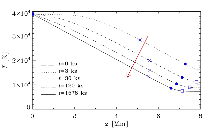
Figure 1: Vertical temperature profile at five different times $t=$ 0, 3, 30, 120, and $1578\,{\rm ks}$ for Run A6 with $\tilde{\kappa_{0}}=10^{6}\,\,{\rm Mm}^{-1}\,{\rm cm}^{3}\,{\rm g}^{-1}$. Squares, circles and crosses represent different optical depths $\tau=0.1$, $\tau=1$ and $\tau=10$, respectively. The arrow represents the direction of the time evolution of the temperature profile.

After a sufficient amount of running time, a unique equilibrium state is reached and the resulting profiles of temperature, density and entropy have a nearly polytropic stratification in the lower part of the domain and a nearly isothermal stratification in the upper part of the domain. An exception are the runs of Set E where the polytropic index is undefined ($n=0/0$). This will be discussed in more detail in Sect. 3.8. We summarize the important quantities obtained from all runs in Table LABEL:results. These quantities are calculated in the equilibrium state. All runs show a similar evolution of density, temperature and entropy. In the next sections we describe the resulting profiles in more detail.

Table 3: Summary of the runs.

Run $a$ $b$ $n$ $\tilde{\kappa_{0}}$ $z_{\rm top}$ $z_{\tau=1}$ $\rho_{\tau=1}$ $\tau_{\rm adjust}$ $T_{\rm eff}$ $K_{\rm bot}$ A4 1 $-3.5$ 3.25 $10^{4}$ 8 2.8 $1.0\;10^{-4}$ 50 23600 $3.9\;10^{-6}$ A5 1 $-3.5$ 3.25 $10^{5}$ 8 5.2 $1.7\;10^{-5}$ 90 13900 $4.6\;10^{-7}$ A6 1 $-3.5$ 3.25 $10^{6}$ 8 6.6 $2.5\;10^{-6}$ 700 7800 $4.6\;10^{-8}$ A7 1 $-3.5$ 3.25 $10^{7}$ 8 7.4 $3.7\;10^{-7}$ 15000 4400 $4.4\;10^{-9}$ B4 1 0 1.5 $10^{4}$ 5 1.4 $2.2\;10^{-4}$ 40 26600 $4.53\;10^{-6}$ B5 1 0 1.5 $10^{5}$ 5 2.9 $9.0\;10^{-5}$ 60 16300 $5.15\;10^{-7}$ B6 1 0 1.5 $10^{6}$ 5 3.8 $3.7\;10^{-5}$ 400 9300 $5.38\;10^{-8}$ B7 1 0 1.5 $10^{7}$ 5 4.3 $1.6\;10^{-5}$ 5000 5200 $5.08\;10^{-9}$ C4 1 1 1 $10^{4}$ 4 1 $2.6\;10^{-4}$ 7 27600 $5.1\;10^{-6}$ C5 1 1 1 $10^{5}$ 4 2.3 $1.3\;10^{-4}$ 20 17400 $5.6\;10^{-7}$ C6 1 1 1 $10^{6}$ 4 3.1 $7.0\;10^{-5}$ 200 10100 $6.0\;10^{-8}$ C7 1 1 1 $10^{7}$ 4 3.4 $3.9\;10^{-5}$ 2100 5700 $6.1\;10^{-9}$ D4 1 5 $-1$ $10^{4}$ 2 0.2 $3.6\;10^{-4}$ 6 31000 $1.1\;10^{-5}$ D5 1 5 $-1$ $10^{5}$ 2 0.8 $2.8\;10^{-4}$ 7 23100 $1.3\;10^{-6}$ D6 1 5 $-1$ $10^{6}$ 2 1 $2.8\;10^{-4}$ 80 15600 $1.9\;10^{-7}$ D7 1 5 $-1$ $10^{7}$ 2 1 $3.2\;10^{-4}$ 700 10100 $3.1\;10^{-8}$ E4 $-1$ 3 0/0 $10^{4}$ 4 3.0 $8.7\;10^{-5}$ 6 23700 $4.47\;10^{-6}$ E5 $-1$ 3 0/0 $10^{5}$ 4 3.6 $5.6\;10^{-5}$ 45 14900 $4.47\;10^{-7}$ E6 $-1$ 3 0/0 $10^{6}$ 4 3.8 $3.9\;10^{-5}$ 400 8800 $4.47\;10^{-8}$

3.1 Approach toward the final state

As mentioned above, we find it convenient to obtain equilibrium solutions by starting from an isothermal state. The upper layers begin to cool fastest, and eventually an equilibrium state is reached. We plot the evolution of the temperature profile of Run A6 in Fig. 1 as an exemplary case with $\tilde{\kappa_{0}}=10^{6}\,\,{\rm Mm}^{-1}\,{\rm cm}^{3}\,{\rm g}^{-1}$. Already after a short time of $t=3\,{\rm ks}$ (1 hours), the temperature has decreased by more than half its initial value at the top and follows a polytropic solution in most of the domain, where the temperature gradient has a similar value than in the equilibrium state. At $t=30\,$ks (8 hours), close to the top boundary, an isothermal part is seen to emerge. However, it takes more than $t=1500\,$ks (17 days) until the equilibrium solution is reached with a prominent isothermal part of $T\approx 7000\,$ K. The locations of three different optical depths, $\tau=0.1,\,1$ and $10$, are shown in Fig. 1. Here,

$$\tau(z)=\int_{z}^{z_{\rm top}}\kappa(z^{\prime})\rho(z^{\prime})\,{\rm d}{}z^{\prime}$$ (17)

is the optical depth with respect to the surface of the domain. If the domain is tall enough, one can see that an initially isothermal stratification cools down first near the location where $\tau(z)\approx 1$, which is where the cooling is most efficient. As an example we plot in Fig. 2 the early stages of the temperature evolution at $t=0$, 0.01, 0.1, and $0.2\,{\rm ks}$ for a taller variant of Run A6 with $z_{\rm top}=12\,{\rm Mm}$ using 1024 equally spaced grid points.

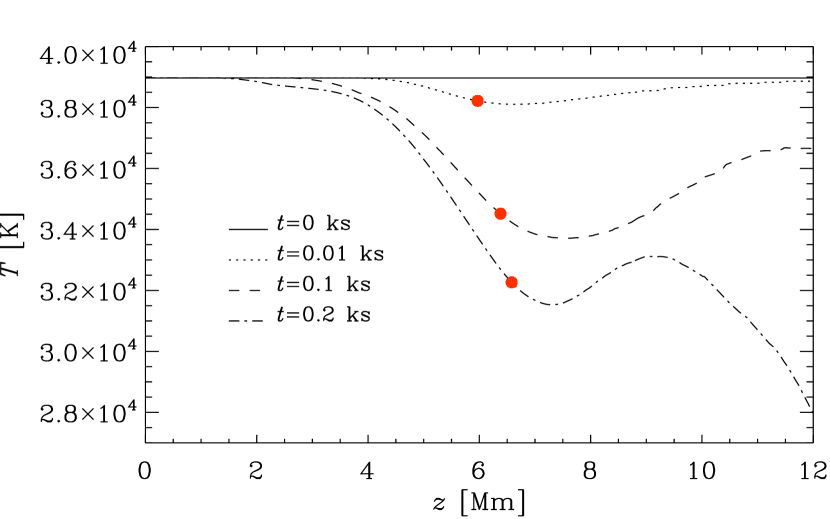
Figure 2: Temperature over height for Run A6 at different times $t=0$, $0.01$, $0.1$, and $0.2\,$ks, plotted as solid, dotted, dashed and dashed-dotted lines, respectively. The red dots correspond to the location of $\tau\approx 1$.

At $t=0.01\,{\rm ks}$, the temperature starts to decrease at the height where $\tau\approx 1$, while in the upper part, which is far enough from the surface, the temperature remains at first unchanged. Only at a somewhat later time ($t=0.1\,{\rm ks}$) does the temperature at $z=12\,{\rm Mm}$ start to cool down. This is explained by the fact that the radiative cooling rate (or inverse cooling time) is largest near $\tau=1$ (Spiegel, 1957; Unno & Spiegel, 1966; Edwards, 1990); see also Appendix A.

3.2 Temperature stratification

For all runs, the temperature reaches an equilibrium state after a certain time; see Fig. 1. The temperature profile can be divided into two distinguishable parts, a nearly polytropic part which starts from the bottom of the domain and extends to a certain height, and a nearly isothermal part which starts from this height and extends to the top of the domain. The transition of the temperature from the initial state to the equilibrium state follows a specific pattern, which is the same for all the runs. The higher the value of $\tilde{\kappa_{0}}$, the lower the temperature is in the isothermal part and the longer it takes to reach this state. Increasing the normalized opacity $\tilde{\kappa_{0}}$ by three orders of magnitude results in a decrease in the temperature by a factor of five for Set A and a factor of three for Set D. As the exponent $b$ changes from the smallest value in Set A to the largest one in Set D, the slope of the temperature decreases with height. This means that the polytropic part of the atmosphere is smaller for larger values of $b$. We note that the size of the domain is chosen larger for smaller values of $b$. For Sets A, B and C, the temperature in the polytropic part is almost the same for different values of $\tilde{\kappa_{0}}$, although for the lowest value of $\tilde{\kappa_{0}}$ the temperature deviates somewhat. However, in Set D, for different values of $\tilde{\kappa_{0}}$, the slope of the temperature is different for each value of $\tilde{\kappa_{0}}$. This has to do with the fact that in this case with $(b-3)/(1+a)=-1$ the stratification is no longer a polytropic one. (A polytrope with $n=-1$ would have constant pressure, which is unphysical.)

The temperatures in the isothermal part also show a dependency on $b$. For $\tilde{\kappa_{0}}=10^{4}\,\,{\rm Mm}^{-1}\,{\rm cm}^{3}\,{\rm g}^{-1}$ the temperature in Run A4 is $T\approx 2.2\;10^{4}\,$K, whereas in Run D4 the value is $T\approx 2.9\;10^{4}\,$K. A similar behavior can also be seen for the other values of $\tilde{\kappa_{0}}$.

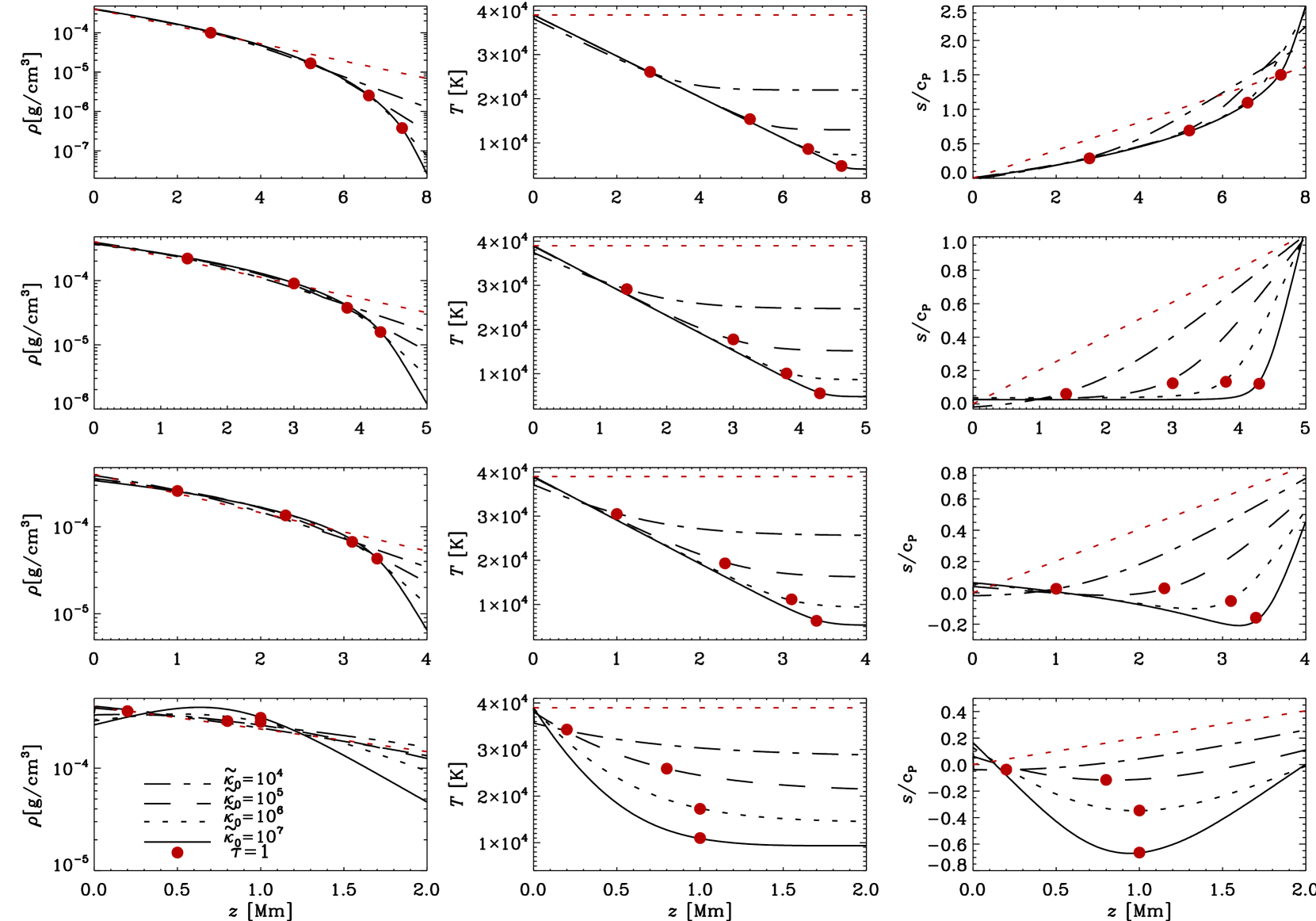
Figure 3: Density, temperature and entropy of the equilibrium state versus height, from left to right, for Sets A, B, C and D, from top to bottom. The four different lines in each plot corresponds to the value of the rescaled opacity $\tilde{\kappa_{0}}=10^{4}$, $10^{5}$, $10^{6}$, $10^{7}\,\,{\rm Mm}^{-1}\,{\rm cm}^{3}\,{\rm g}^{-1}$. The dots in all plots represent the surface $\tau\approx 1$. The red dotted lines represent the initial profile of each set.

Next, we calculate the optical depth for all runs. We find that the transition point from the polytropic part to the isothermal part coincides with the $\tau\approx 1$ surface. We indicate the surface $\tau\approx 1$ by dots in all plots in Fig. 3. The polytropic part corresponds to the optically thick part with $\tau>1$ and the isothermal part corresponds to the optically thin part with $\tau<1$. For each set, the transition point depends on the value of $\tilde{\kappa_{0}}$. As we go from smaller to larger values of $\tilde{\kappa_{0}}$, the surface shifts to larger heights and becomes cooler. This is because the radiative heat conductivity $K$ is inversely proportional to $\tilde{\kappa_{0}}$ and directly proportional to the flux. Therefore, by increasing the value of $\tilde{\kappa_{0}}$, $K$ decreases and, as a consequence, the radiative flux also decreases. By decreasing the flux, the effective temperature decreases as $T_{\rm eff}\propto F_{\rm rad}^{1/4}$. This means that the temperature at the surface is smaller for larger values of $\tilde{\kappa_{0}}$. For Set A, the $\tau\approx 1$ surfaces lie on the polytropic part of the temperature profile. However, by increasing the value of $b$, the locations of the $\tau=1$ surfaces shift toward the lower boundary and the optically thick part becomes narrower. This is particularly severe for the solutions with a small value of $\tilde{\kappa_{0}}$, especially for $\tilde{\kappa_{0}}=10^{4}\,\,{\rm Mm}^{-1}\,{\rm cm}^{3}\,{\rm g}^{-1}$, when the boundary condition $T=T_{\rm bot}$ at $z=0$ becomes unphysical and the temperature drops between the first two meshpoints in a discontinuous fashion; see Fig. 3.

3.3 Entropy stratification

We plot the entropy profiles for all sets of runs in the equilibrium state in the last column of Fig. 3. For Runs C6–7 and D5–7, the entropy decreases in the polytropic part and starts to increase in the isothermal part. All runs show a positive vertical entropy gradient in the isothermal part. In the lower part, the entropy gradient is positive ($\nabla_{z}s>0$) for Set A, while for Set B it is constant and equal to zero ($\nabla_{z}s\approx 0$). This shows that for Set B, the atmospheres are isentropic. In Sets C and D, except for the case $\tilde{\kappa_{0}}=10^{4}\,\,{\rm Mm}^{-1}\,{\rm cm}^{3}\,{\rm g}^{-1}$, the entropy gradient is negative, $\nabla_{z}s<0$. This means that their atmospheres are convectively unstable. (Convection will of course not occur in our one-dimensional model, but we will obtain the so-called hydrostatic reference solution that is used to compute the Rayleigh number, as will also be done later in this paper.) In Set D the entropy gradients are larger than in case C where their atmospheres are marginally stable. In the isothermal part of Set C, the entropy gradient is much larger than in Set D. For each set of runs, as we go from smaller values of $\tilde{\kappa_{0}}$ to larger ones, the entropy profiles have larger gradients.

3.4 Incoming and outgoing intensity profiles

It is instructive to inspect the vertical profiles of the intensity for rays pointing in the up- and downward directions, $\hat{\mbox{\boldmath$n$}}{}=(0,0,\pm 1)$, denoted in the following by $I^{\pm}$. If we have just these two rays, the energy flux is given by $F_{\rm rad}=(2\pi/3)(I^{+}-I^{-})$. In thermal equilibrium, the difference between $I^{+}$ and $I^{-}$ must be constant. This is indeed the case; see Fig. 4, where we plot $I^{+}$ and $I^{-}$ and compare with $S$. The vertical lines in this figure represents the difference between $I^{+}$ and $I^{-}$, where $I^{+}-I^{-}\approx 10^{4}\,$ $\,{\rm erg}\,{\rm cm}^{-2}\,{\rm s}^{-1}$ in the whole domain as we have radiative equilibrium $\mbox{\boldmath$\nabla$}{}\cdot\mbox{\boldmath$F$}{}_{\rm rad}=0$. Radiative equilibrium also demands that $J=S$, so $S$ has to be equal to the average of $I^{+}$ and $I^{-}$, which is indeed the case.

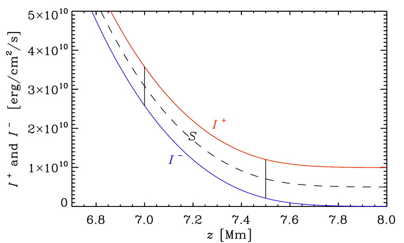
Figure 4: Source function and vertical profiles of incoming and outgoing intensity near the surface for Run A7. The dashed line represents the source function and the solid lines represent the incoming intensity $I^{+}$ (red) and outgoing intensity $I^{-}$ (blue). The vertical lines represent the (constant) difference between $I^{+}$ and $I^{-}$.

3.5 Radiative heat conductivity

In Sets A, B, and C, the value of radiative heat conductivity $K$ turns out to be constant in the optically thick part of the atmosphere, but not for Set D. The value of $K$ at the bottom of the optically thick part of the domain is denoted in Table LABEL:results by $K_{\rm bot}$, and agrees roughly with

$$K_{\rm bot}\approx K_{0}\equiv{16\sigma_{\rm SB}T_{0}^{3}\over 3\tilde{\kappa_{0}}\rho_{0}}.$$ (18)

Indeed, it has almost the same order of magnitude for A, B and C, independently of the value of $b$, but it is one order of magnitude larger for Set D. This is because in this set the density is lower in the optically thick part compared to the other sets. Moreover, as we go from higher values of $\tilde{\kappa_{0}}$ to the lower ones, the radiative heat conductivity increases. This can be explained by the inverse proportionality of $K$ with opacity as $K\propto 1/\tilde{\kappa_{0}}$. For smaller values of $\tilde{\kappa_{0}}$, $K$ is larger and vice versa. As an example, we plot in Fig. 5 the resulting vertical profiles of radiative heat conductivity for Set C. We note that $K$ is constant in the optically thick part and starts to increase in the optically thin part. In the optically thin part, $\kappa\rho$ decreases, so $K$ increases as $K\propto 1/\kappa\rho$. To maintain $\mbox{\boldmath$\nabla$}{}\cdot\mbox{\boldmath$F$}{}_{\rm rad}=0$, the modulus of $\mbox{\boldmath$\nabla$}{}T$ has to decrease. As $K$ increases even further, a thermostatic equilibrium can be satisfied if $\mbox{\boldmath$\nabla$}{}T$ comes close to zero.

Figure 5: Radiative heat conductivity $K$ versus height for Set C. $K$ is plotted for different values of $\tilde{\kappa_{0}}$ where $\tilde{\kappa_{0}}=10^{4}\,\,{\rm Mm}^{-1}\,{\rm cm}^{3}\,{\rm g}^{-1}$ is shown by dotted-dashed line, $\tilde{\kappa_{0}}=10^{5}\,\,{\rm Mm}^{-1}\,{\rm cm}^{3}\,{\rm g}^{-1}$ dashed line, $\tilde{\kappa_{0}}=10^{6}\,\,{\rm Mm}^{-1}\,{\rm cm}^{3}\,{\rm g}^{-1}$ dotted line and $\tilde{\kappa_{0}}=10^{7}\,\,{\rm Mm}^{-1}\,{\rm cm}^{3}\,{\rm g}^{-1}$ solid line.

3.6 Effective temperature

The effective temperature $T_{\rm eff}$ of all runs is calculated from the $z$ component of the radiative flux $\mbox{\boldmath$F$}{}_{\rm rad}$,

$$T_{\rm eff}=\bigg{(}{F_{\rm rad}\over\sigma_{\rm SB}}\bigg{)}^{1/4}.$$ (19)

The values of $T_{\rm eff}$ of all sets of runs are summarized in Table LABEL:results. By increasing the value of $b$, $T_{\rm eff}$ also increases. The value of $T_{\rm eff}$ decreases as we go from lower to higher opacities for each set. We plot $T_{\rm eff}$ versus $\tilde{\kappa_{0}}$ in Fig. 6 for Sets A, C and D where the values of $T_{\rm eff}$ are represented by crosses, circles and stars, respectively. For each set of runs, we fit a line to $T_{\rm eff}$ versus $\tilde{\kappa_{0}}$. We find that $T_{\rm eff}$ has a power law relation with $\tilde{\kappa_{0}}$. The power of $\tilde{\kappa_{0}}$, which is the slope of the plot, depends on the polytropic index and therefore on $b$. For larger values of $b$, the power is smaller than for smaller values of $b$. Additionally, the offset shows also a weak dependence on $b$. A power law relation between $T_{\rm eff}$ and the opacity of roughly $1/4$ can be expected, because of the linear relation of the radiative flux and the opacity. Toward larger $b$, this dependency is no longer accurate. We also calculate for each run the corresponding optical depth where $T=T_{\rm eff}$. For all runs, $T_{\rm eff}$ corresponds to the optical depth $\tau\approx 1/3$. This is less than what is expected for a gray atmosphere, where $T_{\rm eff}=T$ at $\tau\approx 2/3$. This is presumably because in our integration of $\tau$ we have not included the contribution between $\infty$ and $z=z_{\rm top}$.

3.7 Thermal adjustment time

In our simulations we define a thermal adjustment time $\tau_{\rm adjust}$ as the time it takes for each run to reach its numerically obtained final equilibrium temperature in the isothermal part to within $1\%$ (see Fig. 7). The unit of $\tau_{\rm adjust}$ is ks (see Sect. 2.5). The value of $\tau_{\rm adjust}$ for all runs is summarized in Table LABEL:results. As we can see in Table LABEL:results, the thermal adjustment time becomes smaller for larger $b$ and smaller $n$. For each set of runs, $\tau_{\rm adjust}$ grows approximately linearly with $\tilde{\kappa_{0}}$, although for $\tilde{\kappa_{0}}\mathrel{\mathchoice{\vbox{\offinterlineskip\halign{\hfil$\displaystyle#$\hfil\cr<\cr\sim\cr}}}{\vbox{\offinterlineskip\halign{\hfil$\textstyle#$\hfil\cr<\cr\sim\cr}}}{\vbox{\offinterlineskip\halign{\hfil$\scriptstyle#$\hfil\cr<\cr\sim\cr}}}{\vbox{\offinterlineskip\halign{\hfil$\scriptscriptstyle#$\hfil\cr<\cr\sim\cr}}}}10^{5}\,{\rm Mm}^{-1}\,{\rm cm}^{3}\,{\rm g}^{-1}$, the dependency is more shallow. For larger values of $\tilde{\kappa_{0}}$, $\tau_{\rm adjust}$ seems to have a stronger dependency on $b$. We speculate that the reason for increasing the value of $\tau_{\rm adjust}$ for higher values of $\tilde{\kappa_{0}}$ is that by increasing the opacity the energy transport via radiation becomes less efficient as the mean free path of the photon decreases. But it seems that there exists a threshold of efficiency, leading to a larger adjustment time for the lowest values of $\tilde{\kappa_{0}}$, as expected.

We plot the vertical dependence of the mean free path of the photons $\ell=1/\kappa\rho$ normalized by the size of the domain $L$ for Set C.

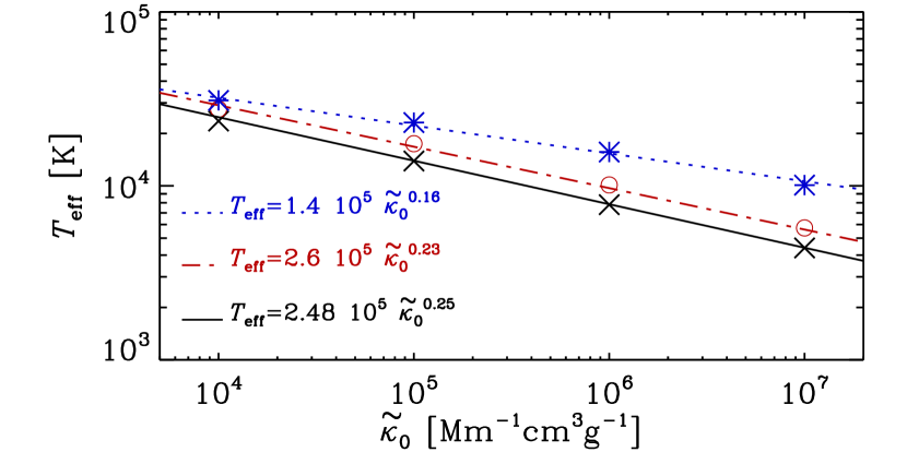
Figure 6: Effective temperature $T_{\rm eff}$ versus rescaled opacity $\tilde{\kappa_{0}}$ for Sets A, C, and D. The crosses, circles and stars show the values of $T_{\rm eff}$ for different values of $\tilde{\kappa_{0}}$ for Sets A, C, and D, respectively. Different lines correspond to line fit of $T_{\rm eff}$ with normalized opacity $\tilde{\kappa_{0}}$.

Figure 7: Temperature $T$ at $z_{\rm top}=4\,{\rm Mm}$ versus time $t$ for Run C5. The two horizontal lines mark the 1% margin around the final value of $T$ and the vertical line marks the time $\tau_{\rm adjust}\approx 20\,{\rm ks}$ after which $T$ lies within these margins.

Figure 8: Normalized mean free path of photons $\ell/L$ versus height for Set C. The dots represent the surface $\tau\approx 1$.

As we can see in Fig. 8, the mean free path increases by several orders of magnitude from the bottom of the domain to the top. Furthermore, $\ell$ is larger for smaller $\tilde{\kappa_{0}}$. In the optically thick part, the difference in $\ell$ is one order of magnitude, which is equal to a corresponding change in $\tilde{\kappa_{0}}$. In the optically thin part, the difference in the values of $\ell$ becomes smaller, as we reach the top of the domain. For $\tilde{\kappa_{0}}=10^{7}\,\,{\rm Mm}^{-1}\,{\rm cm}^{3}\,{\rm g}^{-1}$, $\ell$ is the smallest and, at the bottom of the domain, three orders of magnitude smaller than for $\tilde{\kappa_{0}}=10^{4}\,\,{\rm Mm}^{-1}\,{\rm cm}^{3}\,{\rm g}^{-1}$. Furthermore, $\ell$ is 10 times the size of the domain for $\tilde{\kappa_{0}}=10^{4}\,\,{\rm Mm}^{-1}\,{\rm cm}^{3}\,{\rm g}^{-1}$, which makes the cooling more efficient. We would have expected to see a large change in the mean free path as we go through the surface. Nevertheless, the exponential growth seems to be roughly the same throughout the domain, at least for the smallest value of $\tilde{\kappa_{0}}$.

3.8 Properties of an atmosphere with undefined $n$

By choosing $a=-1$ and $b=3$, we have a constant heat conductivity $K$ that is independent of density and temperature as the heat conductivity is given by Eq. (7). The nominal value of $n$ is given by

$$n={3-3\over 1-1}={0\over 0}.$$ (20)

In this case, since $K={\rm const}{}$, we expect to have only a polytropic solution which satisfies the thermostatic equilibrium if $\nabla_{z}T=$ const, but it is then unclear how $\rho$ varies. In Fig. 9, we plot the profiles of density, temperature and entropy for all three runs of Set E.

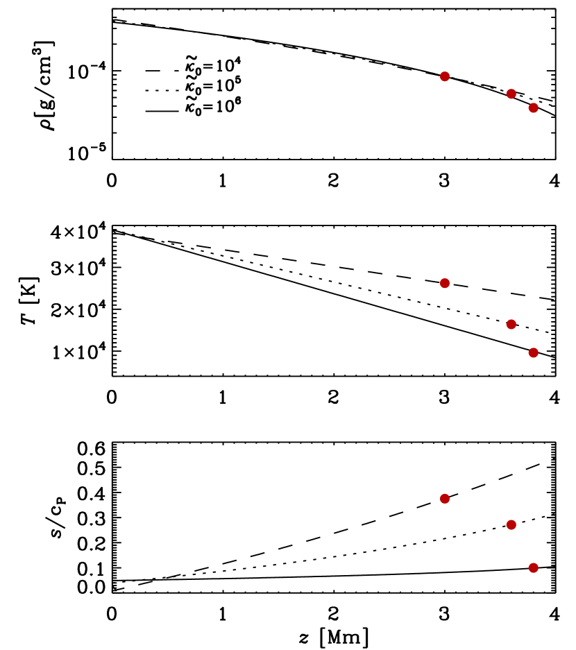
Figure 9: Density, temperature, and entropy profiles for Set E ($n=0/0$). Dashed, dotted, and solid lines represent E4, E5, and E6, respectively. The red dots present the surface of the model where $\tau=1$.

The first panel shows that in the optically thick part the density is nearly the same for the three values of $\tilde{\kappa_{0}}$, while in the optically thin part it decreases with increasing $\tilde{\kappa_{0}}$. For higher values of $\tilde{\kappa_{0}}$, the density drops faster than in the case of smaller $\tilde{\kappa_{0}}$. In all cases, $K$ is constant in both the optically thick and thin parts, but an interesting aspect is that its bottom value $K_{\rm bot}$ is of the same order of magnitude as in Sets A, B, and C. In the second panel of Fig. 9, we plot the temperature profiles. As expected, there is no isothermal part. The slope of temperature decreases approximately linearly as we go to higher values of $\tilde{\kappa_{0}}$, because $K$ is proportional to $1/\tilde{\kappa_{0}}$. Although the solutions show no transition from the polytropic part to an isothermal one, the atmosphere has still a layer where $\tau=1$, which is shown as red dots in all panels of Fig. 9. In contrast to the other sets, A, B, C, and D, the temperature profiles look qualitatively different. As in Sets A, B, and C, in the optically thick part, the different temperature profiles have nearly the same gradient, while in Set E, the gradient is different for the three values of $\tilde{\kappa_{0}}$. This is because in this case, thermostatic equilibrium is obeyed with a constant value of $K$ (independent of $z$).

In the third panel of Fig. 9, we plot entropy profiles for the three values of $\tilde{\kappa_{0}}$. In all cases the entropy increases with a slope that depends on $\tilde{\kappa_{0}}$.

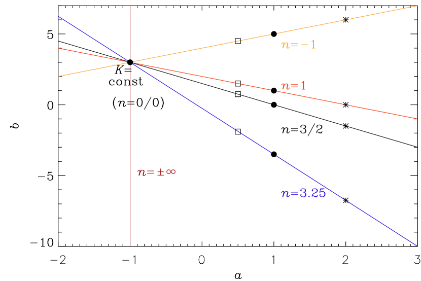
Figure 10: $b$ versus $a$ for different values of the polytropic index $n$. The black dots represents the combination of $a=1$ with different values of $b$ which are used in the main simulation; see Table LABEL:results. The stars represent the combination of $a=2$ and squares represent $a=0.5$ with different values of $b$; see Table LABEL:test-n.

The actual polytropic index can be computed from the resulting super-adiabatic (or entropy) gradient,

$$\nabla-\nabla_{\rm ad}={{\rm d}{}(s/c_{\rm p})\over{\rm d}{}\ln p},$$ (21)

where $\nabla_{\rm ad}=1-1/\gamma$ is the adiabatic gradient. This gives $\nabla$, which is related to the actual $n$ via

$$n_{\rm actual}={{\rm d}{}\ln\rho\over{\rm d}{}\ln T}={{\rm d}{}\ln p\over{\rm d}{}\ln T}-1=\nabla^{-1}-1,$$ (22)

which follows from the perfect gas relation $p\propto\rho T$. We note also that convection is not possible in one dimension, so we obtain directly the hydrostatic solution, which may be unstable.

By solving Eq. (8) for $b$, we obtain $b=3-n(1+a)$; see Fig. 10. We see that for different values of $n$, the graphs of $b$ versus $a$ intersect each other at one common point. This corresponds to $K=K_{0}={\rm const}{}$; see Eq. (7). This means that the solution for constant $K$ can belong to any of these polytropic indexes. For $a=-1$ and $b=3$, in which case $n$ is undefined, the solutions have a value of $n_{\rm actual}$ that depends on the height of the domain. Using Eq. (22) together with hydrostatic equilibrium, ${\rm d}{}p/{\rm d}{}z=-\rho g$, we find

$$n_{\rm actual}=g\,{\mu\over{\cal R}}\,{z_{\rm top}-z_{\rm bot}\over T_{\rm bot}-T_{\rm top}}-1,$$ (23)

so $n_{\rm actual}$ increases as $z_{\rm top}$ is increased. However, this increase is partially being compensated by a small simultaneous decrease of $T_{\rm top}$, which reduces the increase of $n_{\rm actual}$ by about 10% as $z_{\rm top}$ increases. When the domain is sufficiently thin, the value of $n_{\rm actual}$ drops below the critical value $(\gamma-1)^{-1}=3/2$, so the system would be unstable to the onset of convection. We return to the relation between $n$ and the height of the domain in Sect. 3.12, where we consider solutions using the optically thick approximation with a radiative boundary condition at the top.

3.9 Dependence on the size of the domain

In our model, the size of the domain plays an important role in getting the polytropic and isothermal solutions for the temperature profile. The domain has to be big enough so that the transition point lies inside the domain. In Fig. 11, we show the vertical dependence of temperature for six domain sizes for Run A5. If the size of the domain is $z<7\,{\rm Mm}$, it is too small to obtain the isothermal part where $\nabla_{z}T=0$ and a boundary layer is produced. The opacity is then too large to let the heat be radiated away. A size of around $z=8\,{\rm Mm}$ is sufficient to get the isothermal part. However, a domain size that is too large ($z=10\,{\rm Mm}$) leads to numerical difficulties near the top boundary, especially if the resolution is too low. For all the runs shown in Table LABEL:results, we have always started by performing several test simulations to find a suitable domain size.

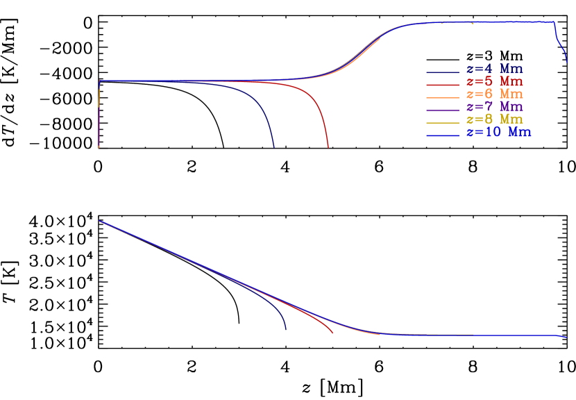
Figure 11: Temperature gradient (upper panel) and temperature profile (lower panel) of seven different sizes of the domain $z=3$, 4, 5, 6, 7, 8, and $10\,{\rm Mm}$ of Run A5. We note that the lines for $z\geq 6$ all fall on top of each other.

3.10 Radiative diffusivity

In numerical simulations, the radiative diffusivity $\chi$ is an important parameter, and has the same dimension as the kinematic viscosity $\nu$. Both $\chi$ and $\nu$ determine whether the results of numerical turbulence simulations are reliable or not and whether they are able to dissipate all the energy within the mesh. In a numerical simulation we are restricted to a certain number of grid points. If the diffusion of the temperature in a simulation is very small, it can happen that the changes in the temperature are too large over the distance of neighboring grid points. Hence, the changes in the temperature cannot be resolved in such a simulation. Therefore, it is important to measure how large are the thermal diffusivity in our models of a radiative atmosphere. The Péclet number is a dimensionless number that quantifies the importance of advective and diffusive term, which is here defined as

$$\mbox{\rm Pe}=u_{\rm rms}H_{\rm p}/\chi,$$ (24)

where $H_{\rm p}$ is a pressure scale height and $u_{\rm rms}$ is rms velocity. The radiative diffusivity is defined as

$$\chi=K/c_{\rm p}\rho,$$ (25)

where $K$ is evaluated using Eq. (7). As we do not solve for a velocity equation in our model, so we use instead the sound speed, which can be related to $u_{\rm rms}$ via the Mach number $\mbox{\rm Ma}=u_{\rm rms}/c_{\rm s}$. The normalized Péclet number in our simulation $\widetilde{\rm Pe}$ is then given by

$$\widetilde{\rm Pe}\equiv\mbox{\rm Pe}/\mbox{\rm Ma}=c_{\rm s}H_{\rm p}/\chi.$$ (26)

As an example, we plot $\widetilde{\rm Pe}$ for Set C in Fig. 12. As we can see in Fig. 12, $\widetilde{\rm Pe}$ is a large number for the optically thick part and it decreases as we go toward the optically thin part. This can be explained with Eq. (25), where $\chi$ is proportional to $K$. In the optically thin part, $K$ increases, so $\chi$ also increases. As a result, $\widetilde{\rm Pe}$ decreases. Furthermore, $\widetilde{\rm Pe}$ is larger for the larger value of $\tilde{\kappa_{0}}$.

Figure 12: $\widetilde{\rm Pe}$ versus $z$ for Set C using different values of $\tilde{\kappa_{0}}$: $\tilde{\kappa_{0}}=10^{4}\,\,{\rm Mm}^{-1}\,{\rm cm}^{3}\,{\rm g}^{-1}$ (dotted-dashed line), $\tilde{\kappa_{0}}=10^{5}\,\,{\rm Mm}^{-1}\,{\rm cm}^{3}\,{\rm g}^{-1}$ (dashed line), $\tilde{\kappa_{0}}=10^{6}\,\,{\rm Mm}^{-1}\,{\rm cm}^{3}\,{\rm g}^{-1}$ (dotted line) and $\tilde{\kappa_{0}}=10^{7}\,\,{\rm Mm}^{-1}\,{\rm cm}^{3}\,{\rm g}^{-1}$ (solid line).

The quantity $\widetilde{\rm Pe}$ is a measure of the ratio of Kelvin-Helmholtz time to the sound travel time, $\tau_{\rm sound}=d/c_{\rm s}$. In our case, $\tau_{\rm sound}\approx 0.1\,{\rm ks}$. Looking at Fig. 12, one sees that $\widetilde{\rm Pe}$ is proportional to $\tilde{\kappa_{0}}$ and thus proportional to the thermal adjustment time. $\widetilde{\rm Pe}$ depends on $z$, but in the middle of the layer at $z=2\,{\rm Mm}$ we have $\widetilde{\rm Pe}\,\tau_{\rm sound}\approx\tau_{\rm adjust}$. This time is much longer than the response time to general three-dimensional disturbances (Spiegel, 1987).

3.11 The same polytropic index with different $a$ and $b$

As we can see in Fig. 10, for a certain value of the polytropic index, we can choose different combinations of $a$ and $b$. For each value of $n$ that we have in Table LABEL:results, we choose two different other combinations of $a$ and $b$ with the same value of $\tilde{\kappa_{0}}=10^{5}\,\,{\rm Mm}^{-1}\,{\rm cm}^{3}\,{\rm g}^{-1}$ . For example for the polytropic index $n=1$ we choose two other combinations as $a=0.5$ and $b=1.5$ for one set and $a=2$ and $b=0$ for another one (see Table LABEL:test-n). We run eight more simulations with the same initial conditions as in previous runs and we obtain a similar equilibrium solution for the same polytropic index $n$. We calculate the effective temperature and the position where $\tau\approx 1$ as reference parameters with our old runs. The results are summarized in Table LABEL:test-n. For each set of runs with the same polytropic index, we labeled the runs similarly to those in Table LABEL:results.

Table 4: Summary of the results for different values of $a$ and $b$ with the same polytropic index $n$.

Run $a$ $b$ $n$ $z_{\tau=1}$ $T_{\rm eff}$ F1 $0.5$ $-1.9$ $3.25$ $5.3$ 13900 F2 1 $-3.5$ $3.25$ $5.2$ 13900 F3 2 $-6.75$ $3.25$ $5.1$ 13400 G1 $0.5$ $0.75$ $1.5$ $3.2$ 16600 G2 1 0 $1.5$ $2.9$ 16300 G3 2 $-1.5$ $1.5$ $2.7$ 16100 H1 $0.5$ $1.5$ 1 $2.6$ 17100 H2 1 1 1 $2.3$ 17500 H3 2 0 1 $2.1$ 18100 I1 $0.5$ $4.5$ $-1$ $1.1$ 21800 I2 1 5 $-1$ $0.8$ 23100 I3 2 6 $-1$ $0.6$ 23700

As we see in Table LABEL:test-n, for each set of runs the effective temperature does not vary strongly, but there is a systematic behavior. By increasing the value of $a$, the effective temperature increases when $n<3/2$ and decreases when $n\geq 3/2$, but the surface is shifted to the lower part of the domain for all sets. The stratification of temperature and other important properties of these atmospheres can be explained analogously to those of Sets A, B, C and D. As an example, we plot in Fig. 13 the temperature profiles (upper panel) and radiative diffusivity $\chi$ (lower panel) for Set H. In the optically thick part, $\chi$ is the same for different combinations of $a$ and $b$ for the same $n$. However, in the optically thin part, $\chi$ becomes larger for larger values of $a$. This can be explained using Eqs. (7) and (25) to show that in the upper isothermal part, $\chi$ increases with decreasing $\rho$ like $\rho^{-(a+2)}$. Thus, we can conclude that, even though $\chi$ is the same and the solution similar to the optically thick part, there are differences in the optically thin part.

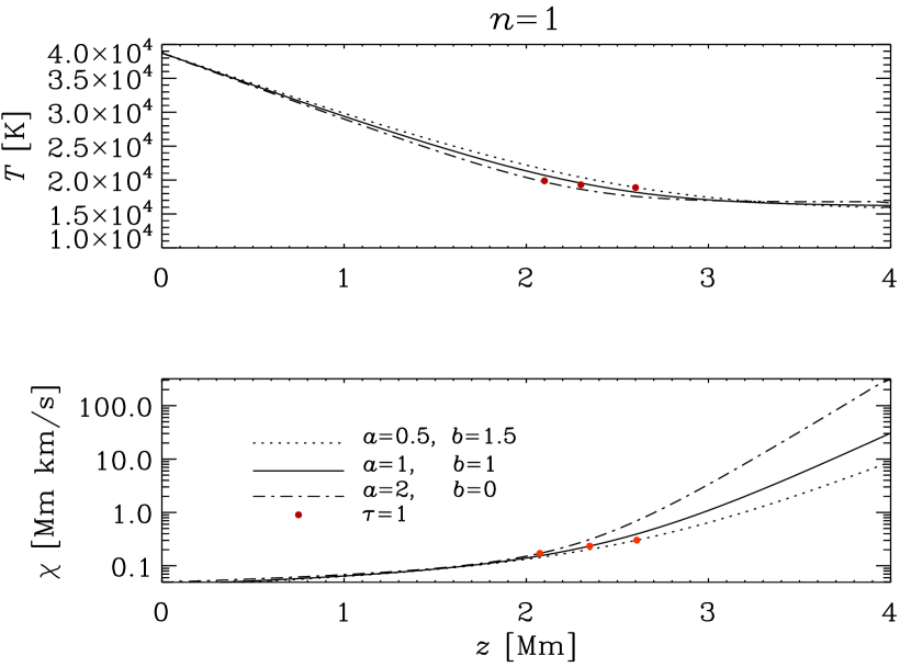
Figure 13: Profile of $T$ and $\chi$ for Set H. In the upper panel, the red dots denote the locations of $\tau=1$.

3.12 Optically thick case with radiative boundary

To compare our results with those in the optically thick approximation, we adopt the radiative boundary condition,

$$-K{{\rm d}{}T\over{\rm d}{}z}=\sigma_{\rm SB}T^{4}\quad\mbox{on $z=z_{\rm top}$},$$ (27)

and keep all other conditions the same as in the radiative transfer calculation, except that $-\mbox{\boldmath$\nabla$}{}\cdot\mbox{\boldmath$F$}{}_{\rm rad}$ in Eq. (3) is replaced by $K\nabla^{2}T$. Here, we have assumed $K$ to be constant, so we shall from now on refer to its value as $K_{0}$, so our solutions will be polytropes with constant polytropic index $n={\rm d}{}\ln\rho/{\rm d}{}\ln T$ and constant double-logarithmic temperature gradient $\nabla={\rm d}{}\ln T/{\rm d}{}\ln p$.

The value of $\nabla=1/(1+n)$ can be computed from the equations governing hydrothermal equilibrium,

$${{\rm d}{}p\over{\rm d}{}z}=-\rho g,\quad{{\rm d}{}T\over{\rm d}{}z}=-{F_{\rm rad}\over K_{0}},$$ (28)

which yields

$$\nabla={{\rm d}{}\ln T\over{\rm d}{}\ln p}={p\over T\rho}\,{F_{\rm rad}\over gK_{0}}=\nabla_{\rm ad}c_{\rm p}\,{F_{\rm rad}\over gK_{0}}.$$ (29)

Such a model is characterized by choosing values for $n$ and $K_{0}$. This is analogous to the case with radiative transfer, where $n$ and $\tilde{\kappa_{0}}$ are specified, and $\tilde{\kappa_{0}}$ is related to $K_{0}$ via Eq. (18). Here, it is convenient to define a non-dimensional radiative conductivity as

$${\cal K}={gK_{0}\over c_{\rm p}\sigma_{\rm SB}T_{\rm bot}^{4}}\,{\nabla\over\nabla_{\rm ad}}.$$ (30)

The radiative flux is then given by

$$F_{\rm rad}=K_{0}\,{g\over c_{\rm p}}\,{\nabla\over\nabla_{\rm ad}}={\cal K}\sigma_{\rm SB}T_{\rm bot}^{4},$$ (31)

so we get the temperature at the top immediately as

$$T_{\rm top}=(F_{\rm rad}/\sigma_{\rm SB})^{1/4}={\cal K}^{1/4}T_{\rm bot}.$$ (32)

Since the temperatures at top and bottom are now known, the thickness of the layer cannot be chosen independently and is instead given by

$$d=(T_{\rm bot}-T_{\rm top})\,K_{0}/F_{\rm rad}={c_{\rm p}\,(T_{\rm bot}-T_{\rm top})\over g\,\nabla/\nabla_{\rm ad}},$$ (33)

which is equivalent to Eq. (23) used before. Again, the fact that the value of $d$ cannot be chosen independently is analogous to the case with radiative transfer, where the thickness of the optically thick layer with nearly constant $K$ emerges as a result of the calculation. In Table LABEL:tkapz we present models for the same parameters as in Table LABEL:results, where $T_{\rm eff}=T_{\rm top}$ in the optically thick model. In agreement with our radiative transfer calculations, we have here treated $\tilde{\kappa_{0}}$ (instead of ${\cal K}$) as our main input parameter (in addition to $n$). We have used Eq. (18) to convert $\tilde{\kappa_{0}}$ into $K_{0}$ and then used Eq. (30) to compute ${\cal K}$. It turns out that there is good agreement regarding the values of $d$, $\rho_{\rm top}$, and $T_{\rm top}$ between the optically thick approximation using a radiative upper boundary condition and the radiative transfer calculations. However, unlike Fig. 6, the data in Table LABEL:tkapz show power law dependence of $T_{\rm eff}$ versus $\tilde{\kappa_{0}}$ with the same exponent of $1/4$ in all cases. To characterize the strength of density and temperature stratification, we also list the ratios $\rho_{\rm bot}/\rho_{\rm top}$ and the ratio of the pressure scale height at the top to the thickness of the layer, $\xi=H_{\rm p}^{\rm top}/d$. As expected, smaller values of $\xi$ are reached by increasing the value of $\tilde{\kappa_{0}}$, but even for $\tilde{\kappa_{0}}=10^{7}\,{\rm Mm}^{-1}\,{\rm cm}^{3}\,{\rm g}^{-1}$ the smallest values of $\xi$ are 0.03 for $n=3.25$ and 0.08 for $n=1$.

Table 5: Summary of model parameters as a function of $n$ and $\tilde{\kappa}_{0}$ as obtained from the optically thick approximation with radiative upper boundary condition.

$n\;\;$ $\tilde{\kappa}_{0}\;$ $d\;\;$ $\rho_{\rm top}\quad\;$ $T_{\rm top}\;$ $\xi\;$ $\rho_{\rm bot}/\rho_{\rm top}$ $3.25$ $10^{4}$ $3.09$ $8.3\;10^{-5}$ $24600$ $0.40$ $4.5$ $3.25$ $10^{5}$ $5.40$ $1.3\;10^{-5}$ $13800$ $0.13$ $28.9$ $3.25$ $10^{6}$ $6.70$ $2.1\;10^{-6}$ $7800$ $0.06$ $187\leavevmode\nobreak\ \leavevmode\nobreak\$ $3.25$ $10^{7}$ $7.44$ $3.2\;10^{-7}$ $4400$ $0.03$ $1220\leavevmode\nobreak\ \leavevmode\nobreak\$ $1.50$ $10^{4}$ $1.37$ $2.2\;10^{-4}$ $28100$ $1.04$ $1.6$ $1.50$ $10^{5}$ $2.93$ $8.9\;10^{-5}$ $15800$ $0.27$ $3.9$ $1.50$ $10^{6}$ $3.80$ $3.8\;10^{-5}$ $8900$ $0.12$ $9.2$ $1.50$ $10^{7}$ $4.30$ $1.6\;10^{-5}$ $5000$ $0.06$ $21.8$ $1.00$ $10^{4}$ $0.94$ $2.8\;10^{-4}$ $29700$ $1.61$ $1.3$ $1.00$ $10^{5}$ $2.25$ $1.4\;10^{-4}$ $16700$ $0.38$ $2.3$ $1.00$ $10^{6}$ $2.99$ $8.0\;10^{-5}$ $9400$ $0.16$ $4.1$ $1.00$ $10^{7}$ $3.41$ $4.5\;10^{-5}$ $5300$ $0.08$ $7.4$

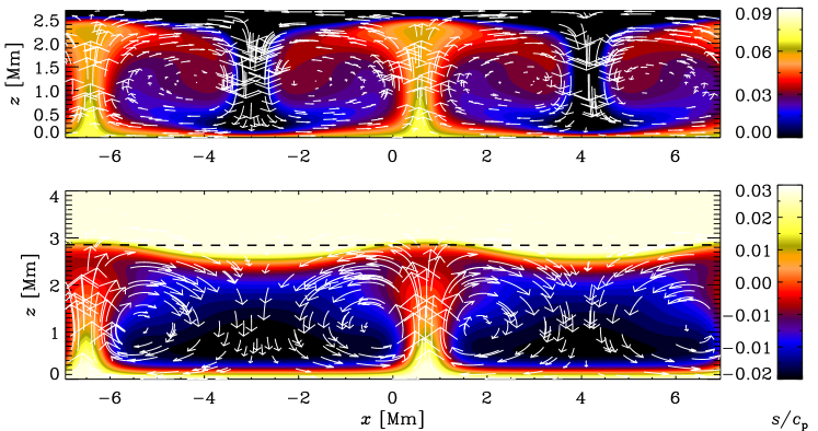
Figure 14: Comparison of velocity and entropy distribution in two-dimensional convection using the optically thick approximation with a radiative upper boundary condition (upper panel) and radiative transfer (lower panel). In both cases we have $\mbox{\rm Pr}=100$ and ${\cal K}=0.01$, corresponding to $\mbox{\rm Ra}=3.6\;10^{4}$. In the lower panel, the dashed line gives the contour $\tau=1$. In order to compare similar structures in the two plots, we have extended the color table of the lower panel to slightly more negative values of $s$ and have clipped it at high values, which are dominated by the strong increase of $s$ above the $\tau=1$ surface.

We emphasize that the only place where the choice of density enters our calculation is in Eq. (18) when we convert $\tilde{\kappa_{0}}$ into $K_{0}$. As already indicated at the end of Sect. 2.5, an increase of $\rho_{0}$ by some factor is equivalent to an increase of $\tilde{\kappa_{0}}$ by the same factor. We note here that $\rho_{0}$ enters both as the initial density at the bottom and in the definition of opacity through Eq. (16). The latter ensures that the opacity only changes through changes in $\tilde{\kappa_{0}}$, and not also through changes in $\rho_{0}$.

3.13 Convection

We now consider two-dimensional convection and compare again results from the optically thick approximation using a radiative upper boundary condition with a calculation using radiative transfer. The control parameter characterizing onset and amplitude of convection is the Rayleigh number,

$$\mbox{\rm Ra}={gd^{4}\over\nu\chi_{\rm mid}}\,\left(-{{\rm d}{}s/c_{\rm p}\over{\rm d}{}z}\right)_{\rm mid},$$ (34)

where $(-c_{\rm p}^{-1}\,{\rm d}{}s/{\rm d}{}z)_{\rm mid}=(\nabla-\nabla_{\rm ad})/H_{\rm p}^{\rm mid}$ is the superadiabatic gradient of the unstable, non-convecting hydrostatic reference solution, and $H_{\rm p}^{\rm mid}=\nabla_{\rm ad}c_{\rm p}T_{\rm mid}/g$ is the pressure scale height in the middle of the optically thick layer. Furthermore, we define the Prandtl number as $\mbox{\rm Pr}=\nu/\chi_{\rm mid}$, where $\nu$ is assumed to be constant and $\chi_{\rm mid}$ is the radiative diffusivity in the middle of the optically thick layer; see Appendix B for details and an example. In Table LABEL:PrRa we list the values of the product Pr Ra, as well as $d$ and $\chi_{\rm mid}$ for models with $n=1$ and different values of ${\cal K}$. We adopt periodic boundary condition in the $x$ direction over a domain with side length $L_{x}$. When we adopt the diffusion approximation we take $z_{\rm top}=d$, where $d$ is calculated from Eq. (33) and given in Table LABEL:PrRa. The mid-layer is then at $z=d/2$, which is also the case when using radiative transfer, where the value of $z_{\rm top}$ ($>d$) was chosen to be sufficiently large and $a=b=1$ is chosen to yield $n=1$ (see Table LABEL:results).

Table 6: Summary of model parameters as a function of ${\cal K}$ for $n=1$.

${\cal K}$ Pr Ra $d$ $\chi_{\rm mid}$ $K_{0}$ $\tilde{\kappa_{0}}$ $5\;10^{-1}$ $7.5\;10^{0}$ $0.63$ $5.6\;10^{-1}$ $6.6\;10^{-6}$ $6.8\;10^{3}$ $2\;10^{-1}$ $\bm{7.1\;10^{2}}$ $1.31$ $2.6\;10^{-1}$ $2.6\;10^{-6}$ $\bm{1.7\;10^{4}}$ $1\;10^{-1}$ $7.7\;10^{3}$ $1.73$ $1.4\;10^{-1}$ $1.3\;10^{-6}$ $3.4\;10^{4}$ $5\;10^{-2}$ $5.9\;10^{4}$ $2.08$ $7.7\;10^{-2}$ $6.6\;10^{-7}$ $6.8\;10^{4}$ $2\;10^{-2}$ $\bm{6.6\;10^{5}}$ $2.46$ $3.3\;10^{-2}$ $2.6\;10^{-7}$ $1.7\;10^{5}$ $\bm{1\;10^{-2}}$ $\bm{3.6\;10^{6}}$ $\!\bm{2.70}\!$ $\!\bm{1.8\;10^{-2}}\!$ $\bm{1.3\;10^{-7}}$ $\bm{3.4\;10^{5}}$ $5\;10^{-3}$ $1.9\;10^{7}$ $2.89$ $9.1\;10^{-3}$ $6.6\;10^{-8}$ $6.8\;10^{5}$ $2\;10^{-3}$ $1.5\;10^{8}$ $3.11$ $3.8\;10^{-3}$ $2.6\;10^{-8}$ $1.7\;10^{6}$ $1\;10^{-3}$ $6.9\;10^{8}$ $3.24$ $1.9\;10^{-3}$ $1.3\;10^{-8}$ $3.4\;10^{6}$ $5\;10^{-4}$ $3.1\;10^{9}$ $3.35$ $9.9\;10^{-4}$ $6.6\;10^{-9}$ $6.8\;10^{6}$ $2\;10^{-4}$ $2.2\;10^{10}$ $3.47$ $4.1\;10^{-4}$ $2.6\;10^{-9}$ $1.7\;10^{7}$ $1\;10^{-4}$ $9.5\;10^{10}$ $3.55$ $2.1\;10^{-4}$ $1.3\;10^{-9}$ $3.4\;10^{7}$

We determine the critical value for the onset of convection by calculating the rms velocity in the domain, $u_{\rm rms}$, for different values of ${\cal K}$ and extrapolate to $u_{\rm rms}\to 0$. For the final to initial bottom density ratio, $\rho_{\rm bot}/\rho_{0}$, we use Eq. (44) derived in Appendix C. Since ${\cal K}$ is proportional to $\chi$ and $\chi_{\rm mid}$, we can compute the product Pr Ra using Eq. (34). It turns out that for $\mbox{\rm Pr}=1$, the critical value is at ${\cal K}\mathrel{\mathchoice{\vbox{\offinterlineskip\halign{\hfil$\displaystyle#$\hfil\cr>\cr\sim\cr}}}{\vbox{\offinterlineskip\halign{\hfil$\textstyle#$\hfil\cr>\cr\sim\cr}}}{\vbox{\offinterlineskip\halign{\hfil$\scriptstyle#$\hfil\cr>\cr\sim\cr}}}{\vbox{\offinterlineskip\halign{\hfil$\scriptscriptstyle#$\hfil\cr>\cr\sim\cr}}}}0.2$ (corresponding to $\mbox{\rm Ra}\mathrel{\mathchoice{\vbox{\offinterlineskip\halign{\hfil$\displaystyle#$\hfil\cr<\cr\sim\cr}}}{\vbox{\offinterlineskip\halign{\hfil$\textstyle#$\hfil\cr<\cr\sim\cr}}}{\vbox{\offinterlineskip\halign{\hfil$\scriptstyle#$\hfil\cr<\cr\sim\cr}}}{\vbox{\offinterlineskip\halign{\hfil$\scriptscriptstyle#$\hfil\cr<\cr\sim\cr}}}}710$) in the optically thick approximation. This corresponds to $\tilde{\kappa_{0}}=1.7\;10^{4}\,{\rm Mm}^{-1}\,{\rm cm}^{3}\,{\rm g}^{-1}$, which is too small to obtain a proper polytropic lower part. Therefore we choose in the following $\mbox{\rm Pr}=100$, in which cases the critical value for the onset of convection is at ${\cal K}\mathrel{\mathchoice{\vbox{\offinterlineskip\halign{\hfil$\displaystyle#$\hfil\cr>\cr\sim\cr}}}{\vbox{\offinterlineskip\halign{\hfil$\textstyle#$\hfil\cr>\cr\sim\cr}}}{\vbox{\offinterlineskip\halign{\hfil$\scriptstyle#$\hfil\cr>\cr\sim\cr}}}{\vbox{\offinterlineskip\halign{\hfil$\scriptscriptstyle#$\hfil\cr>\cr\sim\cr}}}}0.02$ (corresponding to $\mbox{\rm Ra}\mathrel{\mathchoice{\vbox{\offinterlineskip\halign{\hfil$\displaystyle#$\hfil\cr<\cr\sim\cr}}}{\vbox{\offinterlineskip\halign{\hfil$\textstyle#$\hfil\cr<\cr\sim\cr}}}{\vbox{\offinterlineskip\halign{\hfil$\scriptstyle#$\hfil\cr<\cr\sim\cr}}}{\vbox{\offinterlineskip\halign{\hfil$\scriptscriptstyle#$\hfil\cr<\cr\sim\cr}}}}6600$).

In the following, we take ${\cal K}=0.01$, so $\mbox{\rm Ra}=3.6\;10^{4}$, $d=2.70\,{\rm Mm}$, $\nu=1.8\,{\rm Mm}\,{\rm km}\,{\rm s}^{-1}$ (corresponding to $\nu=1.8\;10^{13}\,{\rm cm}^{2}\,{\rm s}^{-1}$), and $\tilde{\kappa_{0}}=3.4\;10^{5}\,{\rm Mm}^{-1}\,{\rm cm}^{3}\,{\rm g}^{-1}$; see the sixth row of Table LABEL:PrRa. We choose $L_{x}=14\,{\rm Mm}$, which is large enough to accommodate two convection cells into the domain; see Fig. 14. The $\tau=1$ surface in the radiative transfer calculation agrees approximately with the height expected from the optically thick models using a radiative upper boundary condition. The flow is only weakly supercritical and therefore not very vigorous, which is also reflected by the fact that the $\tau=1$ surface is nearly flat. In the radiative transfer calculation, the specific entropy increases sharply with height above the $\tau=1$ surface. We note also that the characteristic narrow downdrafts of the optically thick calculation are now much broader when radiation transfer is used. Furthermore, the expected entropy minimum near the surface is virtually absent in the latter case; see also the middle panel of Fig. 15. This is because near $z=d$, the local value of $\chi$ is rather large (see the lower panel of Fig. 13), so the thickness of the thermal boundary layer becomes comparable to $d$ itself.

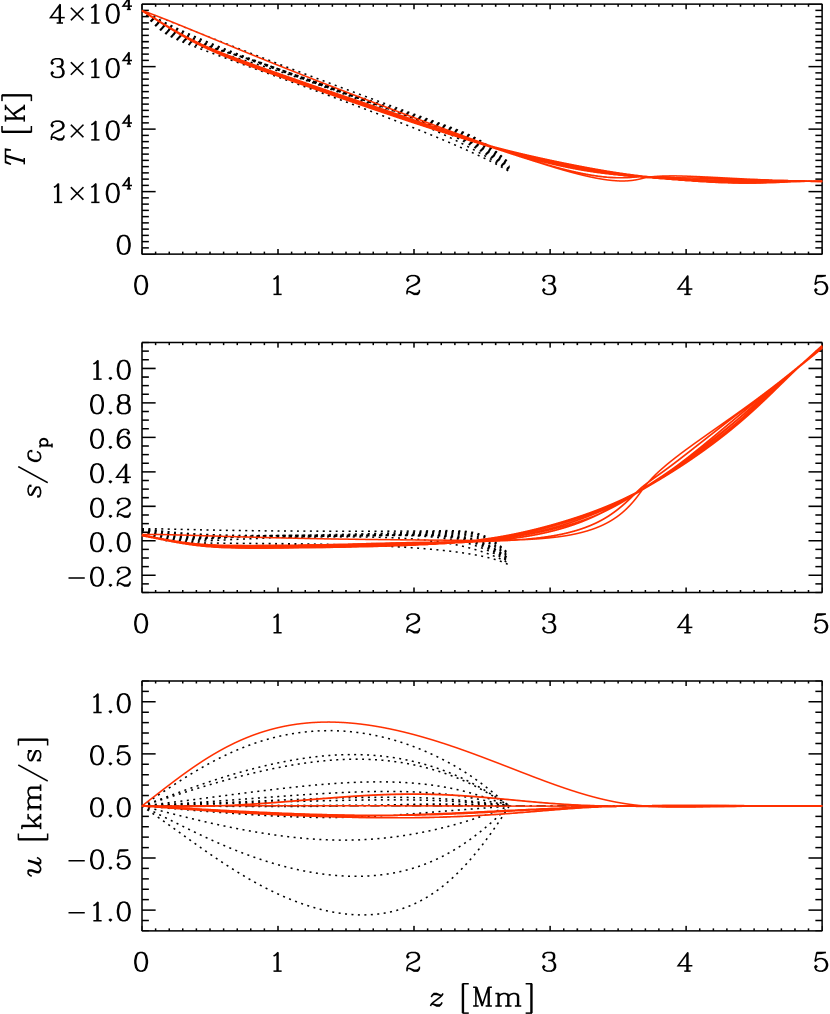
Figure 15: Comparison of vertical temperature, entropy, and velocity profiles at different $x$ positions for the model shown in Fig. 14. The black dotted lines refer to the run with diffusion approximation and radiative upper boundary condition and the red solid lines to the run with radiative transfer.

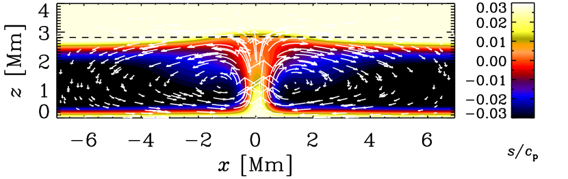
Figure 16: Similar to the lower panel of Fig. 14, but at a later time ($t=500\,{\rm ks}$), when the solution has switched into a single-cell configuration.

In the model using the diffusion approximation, the temperature variations are much larger than in the model with radiative transfer; see Fig. 15. In the latter case, the velocities overshoot into the upper stably stratified layer, and the downflows are much broader and therefore slower than in the diffusion approximation.

It turns out that the solution with radiative transfer shown in Fig. 14 is quasi-stable until about $350\,{\rm ks}$ ($\approx 4$ days) and then switches into a single-cell configuration with a fairly isolated updraft; see Fig. 16. We have seen similar behavior in other cases with radiation too, and it is possible that this is a consequence of our setup. Firstly, the restriction to two-dimensional convection is a serious artifact. Secondly, the assumption of a fixed temperature at the bottom was a mathematical convenience, but it is not physical motivated.

4 Increasing the density contrast

As alluded to in the introduction, the inclusion of the physics of radiation implies the occurrence of $\sigma_{\rm SB}$ as an additional physical constant that couples the resulting temperature and density contrasts to changes in the Rayleigh number. Given that we have already made other simplifications such as the negligence of hydrogen ionization, we end up with rather small density contrasts of less than ten when $n=1$, as seen in Table LABEL:tkapz. By considering $\sigma_{\rm SB}$ an adjustable parameter, we can alleviate this constraint. We demonstrate this in Table 7, where we increase the value of $\sigma_{\rm SB}$ from its physical value of $5.67\;10^{-20}\,{\rm g}\,{\rm cm}^{-3}\,{\rm km}^{3}\,{\rm s}^{-3}\,{\rm K}^{-4}$ by eight orders of magnitude, keeping however $K_{0}$ fixed. We have chosen here $K_{0}=1.3\;10^{-7}=\,{\rm g}\,{\rm cm}^{-3}\,{\rm km}^{3}\,{\rm s}^{-3}\,{\rm Mm}\,{\rm K}^{-1}$, which corresponds to the model in the sixth row of Table LABEL:PrRa. Since $\sigma_{\rm SB}$ enters the definition of ${\cal K}$, its value is now no longer the same, even though $K_{0}$ is. The Rayleigh numbers change slightly, because they depend on the values of density and temperature in the middle of the domain, which do of course change.

Table 7: Density contrast and other model parameters as a function of $\sigma_{\rm SB}$ for $n=1$ and $K_{0}=1.3\times 10^{-7}$.

$\sigma_{\rm SB}\quad\;\;$  Pr Ra $d\;\;\;$ $\chi_{\rm mid}\quad$ $\rho_{\rm bot}/\rho_{\rm top}\!\!\!\!$ $\tilde{\kappa_{0}}$ $5.67\;10^{-20}$ $3.63\;10^{6}$ $2.70$ $1.8\;10^{-2}$ $3.2$ $3.4\;10^{5}$ $5.67\;10^{-18}$ $9.45\;10^{6}$ $3.55$ $2.1\;10^{-2}$ $10.0$ $3.4\;10^{7}$ $5.67\;10^{-16}$ $1.23\;10^{7}$ $3.82$ $2.2\;10^{-2}$ $31.6$ $3.4\;10^{9}$ $5.67\;10^{-14}$ $1.33\;10^{7}$ $3.90$ $2.2\;10^{-2}$ $100.0$ $3.4\;10^{11}$ $5.67\;10^{-12}$ $1.36\;10^{7}$ $3.93$ $2.2\;10^{-2}$ $316.2$ $3.4\;10^{13}$

Large density contrasts are one of the important ingredients in modeling the physics of sunspot formation by surface effects such as the negative effective magnetic pressure instability; see Brandenburg et al. (2013) for a recent model. Including radiation into such still rather idealized models and to study the relation to other competing or corroborating mechanisms such as the one of Kitchatinov & Mazur (2000) was indeed an important motivation behind the work of the present paper.

5 Conclusions

The inclusion of radiative transfer in a hydrodynamic code provides a natural and physically motivated way of placing an upper stably stratified layer on top of an optically thick layer that may be stably or unstably stratified, which of the two depends on the opacity. Using a Kramers-like opacity law with freely adjustable exponents on density and temperature yields polytropic solutions for certain combinations of the exponents $a$ and $b$. The prefactor in the opacity law determines essentially the values of the Péclet and Rayleigh numbers. However, in contrast to earlier studies of convection in polytropic layers, the temperature contrast is no longer a free parameter and increases with increasing Rayleigh number—unless one considers the Stefan–Boltzmann ‘constant’ as an adjustable parameter. The physical values of the prefactor on the opacity are much larger than those used here, but larger prefactors lead to values of the radiative diffusivity that become eventually so small that temperature fluctuations on the mesh scale cannot be dissipated by radiative diffusion. In previous work (Nordlund, 1982; Steffen et al., 1989; Vögler et al., 2005; Heinemann et al., 2007; Freytag et al., 2012), this problem has been avoided by applying numerical diffusion or using numerical schemes that dissipate the energy when and where needed. However, this may also suppress the possibility of physical instabilities that we are ultimately interested in. This motivates the investigation of models with prefactors in the Kramers opacity law that are manageable without the use of numerical procedures to dissipate energy artificially.

It turns out that in all cases with $a$ and $b$ such that $n>-1$, the stratification corresponds to a polytrope with index $n$ below the photosphere and to an isothermal one above it. This was actually expected given that such a solution has previously been obtained analytically in the special case of constant $\kappa$ (corresponding to $a=b=0$); see Spiegel (2006). On the other hand, the isothermal part was apparently not present in the simulations of Edwards (1990).

Contrary to the usual polytropic setups (e.g., Brandenburg et al., 1996), the temperature contrast is now no longer an independent parameter but it is tied essentially to the Rayleigh number. Significant temperature contrasts can only be achieved at large Rayleigh numbers, which corresponds to a large prefactor in front of the opacity. While this aspect can be reproduced already with polytropic models using the radiative boundary conditions, there are some surprising differences between the two. Most important is perhaps the fact that the specific entropy must increase above the unstable layer, while with a radiative boundary condition the specific entropy always decreases. Although the differences in the resulting temperature profiles are small, there are major differences in the flows speeds in the two cases. We also find that at late times the convection cells in simulations with full radiative transport tend to merge into larger ones. Whether or not this is an artefact of our restriction to two-dimensional flows remains open. In this connection, we should also point out the presence of a geometric correction factor in front of the radiative heating and cooling term in Eq. (15) that is needed to reproduce the correct cooling rate, but it does not affect the steady state solution.

Comparing with realistic simulations of the Sun, there is not really an isothermal part, but a pronounced sudden drop in temperature followed by a continued decrease in temperature (see, e.g., Stein & Nordlund, 1998). On the other hand, in our simulations there is no jump in the temperature profile near the surface and the atmosphere changes smoothly from polytropic to isothermal. We suspect that the reason for this difference is that in our models ionization effects are ignored, while in the solar atmosphere the degree of ionization of hydrogen increases with depth. In the Sun, the density decreases significantly from the upper part of the convection zone as we go to the photosphere. This makes the opacity smaller and the atmosphere in the photosphere becomes transparent. At the height where the ionization temperature of hydrogen is reached, the $H^{-}$ opacity becomes important, which is not included in our simulations. The radiative heat conductivity in our simulations is found to be constant throughout the optically thick part and then increases sharply in the optically thin part. Solving this in the optically thick approximation, which has sometimes been done, becomes computationally expensive and even unphysical, so radiative transfer becomes a viable alternative for studying layers that are otherwise polytropic in the lower part of the domain.

Appendix A Cooling rate and correction factor

The purpose of this appendix is to show that for one-dimensional temperature perturbations, the correct cooling rates are obtained with just two rays if the $D/3$ correction factor in Eq. (15) is applied. Similar considerations apply also to the case of two-dimensional problems. Cooling rates are important for understanding temporal aspects such as the approach to the final state (Sect. 3.1) or the thermal adjustment time (Sect. 3.7). Thus, the equilibrium solutions discussed in the other sections are not affected by the following considerations.

The source of the problem lies in the fact that the $4\pi$ angular integration in Eq. (4) becomes inaccurate in one dimension and dependent on the optical thickness. In the optically thick regime, the diffusion approximation holds, so the cooling rate is proportional to $K$, which has a $1/3$ factor in Eq. (7). In one dimension, one uses only the two rays in the vertical direction, so one misses the $1/3$ factor and has to apply it afterwards to account for the “redundant” rays in the other two coordinate directions that show no variation. This is what is done in Eq. (15). However, in the optically thin limit, the mean free path becomes infinite and cooling is now possible in all three directions. In that case, the one-dimensional approximation is not useful. To explain this in more detail, we begin by considering first the general case of three-dimensional perturbations with wavevector $\bm{k}$ (Spiegel, 1957). In that case, one can use the Eddington approximation to solve the transfer equation for the mean intensity, $J=\int I\,{\rm d}{}\Omega/4\pi$,

$${\textstyle{1\over 3}}\,(\ell\nabla)^{2}J=J-S,$$ (35)

so the cooling rate (for three-dimensional perturbations) is (Unno & Spiegel, 1966; Edwards, 1990)

$$\lambda_{\rm 3D}={16\sigma_{\rm SB}T^{3}\over\rho c_{\rm p}}\,{\kappa\rho\bm{k}^{2}\over 3\kappa^{2}\rho^{2}+\bm{k}^{2}}.$$ (36)

It is convenient to introduce here a photon diffusion speed as

$$c_{\gamma}=16\sigma_{\rm SB}T^{3}/\rho c_{\rm p}$$ (37)

and to write Eq. (36) in the form

$$\lambda_{\rm 3D}={c_{\gamma}\ell\bm{k}^{2}/3\over 1+\ell^{2}\bm{k}^{2}/3},$$ (38)

where $c_{\gamma}\ell/3=\chi$ is the radiative diffusivity, as defined in Eq. (25), and $\ell=1/\kappa\rho$ is the local mean-free path of photons.

Solving Eq. (5) for two rays corresponds to solving Eq. (35) without the $1/3$ factor. We would then obtain Eq. (38) without the two $1/3$ factors. This would evidently violate the well-known cooling rate $\chi\bm{k}^{2}$ in the optically thick limit, but in the optically thin limit it would be in agreement with Eq. (38), because the two $1/3$ factors would cancel for large values of $\ell$. However, we have to remember that temperature perturbations are here assumed one-dimensional, so the intensity can only vary in the $z$ direction, while the rays still go in all three directions. This means that under the sum in Eq. (15) only one third of the $I-S$ terms give a contribution, and that the cooling rate is therefore

$$\lambda_{\rm 1D}={c_{\gamma}\ell k_{z}^{2}/3\over 1+\ell^{2}k_{z}^{2}},$$ (39)

which has now only a single $1/3$ factor. Likewise, if we had two-dimensional perturbations such as in two-dimensional convection considered in Sect. 3.13, only $2/3$ of the terms under the sum in Eq. (15) would contribute. However, in a two-dimensional radiative transfer calculation, the additional $1/3$ would be absent, which explains the $D/3$ correction factor with $D=2$ in this case.

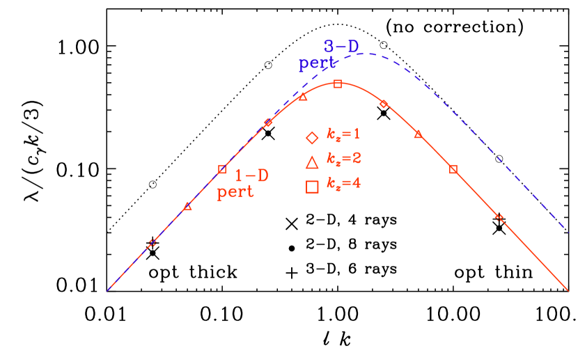
Figure 17: Dependence of the cooling rates computed from models with different values of $\tilde{\kappa_{0}}$ (from $10^{2}$ to $10^{5}$ $\,{\rm Mm}^{-1}\,{\rm cm}^{3}\,{\rm g}^{-1}$) and $k_{z}$ (=1, 2, and 4 indicated by diamonds, triangles, and squares, respectively). 2-D models with four and eight rays are indicated by crosses and circles, respectively, while 3-D models with six rays are shown as plus signs. The red solid line corresponds to Eq. (39), the dashed blue line to Eq. (38), and the dotted line with open circles to the case without correction factor.

We have verified that with the correction factor in place, the code now yields the same cooling rates in both the optically thick and thin regimes, regardless of the numbers of rays used. This is shown in Fig. 17, where we plot cooling rates for different values of $\tilde{\kappa_{0}}$ in a domain of size $2\pi$ (in Mm), so the smallest wavenumber is $1\,{\rm Mm}^{-1}$. With $\rho=4\times 10^{-4}\,{\rm g}\,{\rm cm}^{-3}$ the photon mean-free path varies from 0.025 to 25 $\,{\rm Mm}$ as $\tilde{\kappa_{0}}$ is decreased from $10^{5}$ to $10^{2}$ $\,{\rm Mm}^{-1}\,{\rm cm}^{3}\,{\rm g}^{-1}$. For the Kramers opacity, we use the exponents $a=1$ and $b=0$. (No gravity is included here, so there would be no convection.) The temperature is $38,968\,{\rm K}$, as before, which yields $c_{\gamma}=3.87\,{\rm km}\,{\rm s}^{-1}$ for the photon diffusion speed. There is excellent agreement between 1-D cases with correction factor and the 3-D calculation (with one-dimensional perturbation). However, the 2/3 correction factor in the 2-D calculation (both with four and with eight rays) seems to be systematically off and should instead by around 0.8 for better agreement. However, as discussed before, the correction factor does not affect the steady state and therefore also not the results presented in Sect. 3.13. The diffusion approximation would imply $\lambda=(c_{\gamma}k/3)\ell k=\chi k^{2}$, which corresponds to the diagonal in Fig. 17 and agrees with the red solid line for $\ell k\mathrel{\mathchoice{\vbox{\offinterlineskip\halign{\hfil$\displaystyle#$\hfil\cr<\cr\sim\cr}}}{\vbox{\offinterlineskip\halign{\hfil$\textstyle#$\hfil\cr<\cr\sim\cr}}}{\vbox{\offinterlineskip\halign{\hfil$\scriptstyle#$\hfil\cr<\cr\sim\cr}}}{\vbox{\offinterlineskip\halign{\hfil$\scriptscriptstyle#$\hfil\cr<\cr\sim\cr}}}}0.5$.

For three-dimensional perturbations, the correct cooling rate in the optically thin regime is three times faster than for one-dimensional perturbations. This is because now the radiation goes in all three directions. Solutions to three-dimensional perturbations clearly cannot be reproduced in less than three dimensions. However, for one-dimensional perturbations, the correct cooling rate is now obtained with a one-dimensional calculation both in the optically thin and thick regimes.

Appendix B Expressions for Pr Ra and $\chi_{\rm mid}$

In Table LABEL:PrRa we listed the values of Pr Ra and $\chi_{\rm mid}$ in the middle of the layer. The purpose of this appendix is to give the explicit expressions and to demonstrate the calculation with the help of an example. Since $n=1$ was assumed, we have $\nabla=(1+n)^{-1}=1/2$. Considering the case ${\cal K}=0.01$, Eqs. (31)–(33) yield $F_{\rm rad}=0.00131\,{\rm g}\,{\rm cm}^{-3}\,{\rm km}^{3}\,{\rm s}^{-3}$, $T_{\rm top}=12320\,{\rm K}$, and $d=2.70\,{\rm Mm}$. Next, given that the temperature varies linearly, we compute the mid-layer temperature as $T_{\rm mid}={\textstyle{1\over 2}}(T_{\rm top}+T_{\rm bot})=25600\,{\rm K}$. This allows us to compute $\rho_{\rm mid}=\rho_{\rm bot}\,(T_{\rm mid}/T_{\rm bot})^{n}=2.2\;10^{-4}\,{\rm g}\,{\rm cm}^{-3}$, where $\rho_{\rm bot}=3.3\;10^{-4}\,{\rm g}\,{\rm cm}^{-3}$ is smaller than $\rho_{0}$ by a factor $\rho_{\rm bot}/\rho_{0}=0.83$; see Appendix C. Thus, $\chi_{\rm mid}=F_{\rm rad}/(\rho_{\rm mid}g\nabla/\nabla_{\rm ad})=0.0175\,{\rm Mm}\,{\rm km}\,{\rm s}^{-1}$, as well as $H_{\rm p}^{\rm mid}=\nabla_{\rm ad}c_{\rm p}T_{\rm mid}/g=1.30\,{\rm Mm}$. This yields $\mbox{\rm Pr}\,\mbox{\rm Ra}=gd^{4}/\chi_{\rm mid}^{2}(\nabla-\nabla_{\rm ad})/H_{p}^{\rm mid}=3.6\;10^{6}$, where $\nabla-\nabla_{\rm ad}=0.1$.

Appendix C Final to initial bottom density ratio

Initially, the stratification is isothermal, so the density is given by $\rho(z)=\rho_{0}\exp(-z/H_{\rm p}^{\rm bot})$ and the initial surface density is

$$\Sigma_{\rm ini}=\int_{0}^{d}\rho(z)\,{\rm d}{}z=\rho_{0}H_{\rm p}^{\rm bot}\left[1-\exp(-d/H_{\rm p}^{\rm bot})\right].$$ (40)

In the final state, the stratification is polytropic, so the density is given by $\rho(z)=\rho_{\rm bot}[T(z)/T_{\rm bot}]^{n}$ and the surface density is

$$\Sigma_{\rm fin}=\rho_{\rm bot}\int_{0}^{d}\left[{T(z)\over T_{\rm bot}}\right]^{n}{{\rm d}{}z\over{\rm d}{}T}\,{\rm d}{}T.$$ (41)

Here, $\rho_{\rm bot}$ is the bottom density of the final state, which is different from the initial value $\rho_{0}$, as explained in Sect. 2.6. Integrating Eq. (41) and using ${\rm d}{}z/{\rm d}{}T=K_{0}/F_{\rm rad}$ from Eq. (28) yields

$$\Sigma_{\rm fin}={\rho_{\rm bot}\over n+1}\left[1-\left({T_{\rm top}\over T_{\rm bot}}\right)^{n+1}\right]{K_{0}T_{\rm bot}\over F_{\rm rad}}.$$ (42)

Using Eq. (29) together with $\nabla=1/(1+n)$ and $H_{\rm p}^{\rm bot}=\nabla_{\rm ad}c_{\rm p}T_{\rm bot}/g$, we have

$$\Sigma_{\rm fin}=\rho_{\rm bot}H_{\rm p}^{\rm bot}\left[1-\left({T_{\rm top}\over T_{\rm bot}}\right)^{n+1}\right].$$ (43)

Using mass conservation, we have $\Sigma_{\rm fin}=\Sigma_{\rm ini}$, so we obtain from Eqs. (40) and (43)

$${\rho_{\rm bot}\over\rho_{0}}={1-e^{-d/H_{\rm p}^{\rm bot}}\over 1-(T_{\rm top}/T_{\rm bot})^{n+1}}.$$ (44)

for the final to initial bottom density ratio.

References

- Brandenburg (2005) Brandenburg, A. 2005, ApJ, 625, 539
- Brandenburg et al. (1996) Brandenburg, A., Jennings, R. L., Nordlund, Å., Rieutord, M., Stein, R. F., & Tuominen, I. 1996, J. Fluid Mech., 306, 325
- Brandenburg et al. (2013) Brandenburg, A., Kleeorin, N., & Rogachevskii, I. 2013, ApJL, 776, L23
- Cattaneo et al. (1991) Cattaneo, F., Brummell, N. H., Toomre, J., Malagoli, A., & Hurlburt, N. E. 1991, ApJ, 370, 282
- Edwards (1990) Edwards, J. M. 1990, MNRAS, 242, 224
- Gastine & Dintrans (2008) Gastine, T., & Dintrans, B. 2008, A&A, 484, 29
- Freytag et al. (2012) Freytag, B., Steffen, M., Ludwig, H.-G., Wedemeyer-Böhm, S., Schaffenberger, W., & Steiner, O. 2012, J. Comput. Phys., 231, 919
- Heinemann et al. (2006) Heinemann, T., Dobler, W., Nordlund, Å., & Brandenburg, A. 2006, A&A, 448, 731
- Heinemann et al. (2007) Heinemann, T., Nordlund, Å., Scharmer, G. B., & Spruit, H. C. 2007, ApJ, 669, 1390
- Käpylä et al. (2012) Käpylä, P. J., Mantere, M. J., & Brandenburg, A. 2012, ApJL, 755, L22
- Käpylä et al. (2013) Käpylä, P. J., Mantere, M. J., Cole, E., Warnecke, J., & Brandenburg, A. 2013, ApJ, 778, 41
- Kippenhahn & Weigert (1990) Kippenhahn, R., & Weigert, A. 1990, Stellar structure and evolution (Springer: Berlin)
- Kitchatinov & Mazur (2000) Kitchatinov, L. L., & Mazur, M. V. 2000, Solar Phys., 191, 325
- Miesch et al. (2000) Miesch, M. S., Elliott, J. R., Toomre, J., Clune, T. L., Glatzmaier, G. A., & Gilman, P. A. 2000, ApJ, 532, 593
- Mitra et al. (2014) Mitra, D., Brandenburg, A., Kleeorin, N., & Rogachevskii, I. 2014, MNRAS, submitted, arXiv:1404.3194
- Nordlund (1982) Nordlund, Å. 1982, A&A, 107, 1
- Nordlund (1985) Nordlund, Å. 1985, Solar Phys., 100, 209
- Spiegel (1957) Spiegel, E. A. 1957, ApJ, 126, 202
- Spiegel (1987) Spiegel, E. A. 1987, in The internal solar angular velocity, ed. B. R. Durney & S. Sofia (Reidel, Dordrecht), 321
- Spiegel (2006) Spiegel, E. A. 2006, EAS Publ. Ser., 21, 127
- Steffen et al. (1989) Steffen, M., Ludwig, H.-G., & Krüß, A. 1989, A&A, 123, 371
- Stein & Nordlund (1989) Stein, R. F., & Nordlund, Å. 1989, ApJL, 342, L95
- Stein & Nordlund (1998) Stein, R. F., & Nordlund, Å. 1998, ApJ, 499, 914
- Stein & Nordlund (2012) Stein, R. F., & Nordlund, Å. 2012, ApJL, 753, L13
- Warnecke et al. (2013) Warnecke, J., Losada, I. R., Brandenburg, A., Kleeorin, N., & Rogachevskii, I. 2013, ApJL, 777, L37
- Unno & Spiegel (1966) Unno, W., & Spiegel, E. A. 1966, Publ. Astron. Soc. Japan, 18, 85
- Vögler et al. (2005) Vögler, A., Shelyag, S., Schüssler, M., Cattaneo, F., & Emonet, T. 2005, A&A, 429, 335
- Stix (2002) Stix, M. 2002, The Sun: an introduction (Springer-Verlag, Berlin)