Chiral dynamics and peripheral transverse densities

Abstract

In the partonic (or light–front) description of relativistic systems the electromagnetic form factors are expressed in terms of frame–independent charge and magnetization densities in transverse space. This formulation allows one to identify the chiral components of nucleon structure as the peripheral densities at transverse distances $b=O(M_{\pi}^{-1})$ and compute them in a parametrically controlled manner. A dispersion relation connects the large–distance behavior of the transverse charge and magnetization densities to the spectral functions of the Dirac and Pauli form factors near the two–pion threshold at timelike $t=4M_{\pi}^{2}$, which can be computed in relativistic chiral effective field theory. Using the leading–order approximation we (a) derive the asymptotic behavior (Yukawa tail) of the isovector transverse densities in the “chiral” region $b=O(M_{\pi}^{-1})$ and the “molecular” region $b=O(M_{N}^{2}/M_{\pi}^{3})$; (b) perform the heavy–baryon expansion of the transverse densities; (c) explain the relative magnitude of the peripheral charge and magnetization densities in a simple mechanical picture; (d) include $\Delta$ isobar intermediate states and study the peripheral transverse densities in the large–$N_{c}$ limit of QCD; (e) quantify the region of transverse distances where the chiral components of the densities are numerically dominant; (f) calculate the chiral divergences of the $b^{2}$–weighted moments of the isovector transverse densities (charge and anomalous magnetic radii) in the limit $M_{\pi}\rightarrow 0$ and determine their spatial support. Our approach provides a concise formulation of the spatial structure of the nucleon’s chiral component and offers new insights into basic properties of the chiral expansion. It relates the information extracted from low–$t$ elastic form factors to the generalized parton distributions probed in peripheral high–energy scattering processes.

I Introduction

Understanding the spatial structure of hadrons and their interactions is one of the main objectives of modern strong interaction physics. A space–time picture is needed not only to gain a more intuitive understanding of hadrons as extended systems, but also to enable the formulation of approximation methods taking advantage of the relevant distance scales. For non–relativistic quantum systems such as atoms in electrodynamics or nuclei in conventional many–body theory a space–time picture follows naturally from the Schrödinger wave function, resulting in a rich intuition based on concepts like the spatial size of configurations and the orbital motion of the constituents. For essentially relativistic systems such as hadrons the space–time picture is more complex, as the particle number can change due to vacuum fluctuations, the notion of wave function is reference frame–dependent, and constraints like crossing invariance and analyticity need to be satisfied.

The light–front description of relativistic systems provides a framework in which it is possible to formulate a rigorous space–time picture. One way to arrive at this description is to consider the system in a frame where it moves which a large momentum and decouples from the vacuum fluctuations (“infinite–momentum frame”) Weinberg:1966jm ; Kogut:1969xa ; Bjorken:1970ah ; Gribov:1973jg . Another, equivalent way is to view the system at fixed light–front time, which can be done in any frame (“light–front quantization”) Dirac:1949cp ; Leutwyler:1977vy ; Lepage:1980fj ; see Ref. Brodsky:1997de for a review. Either way one obtains a closed quantum–mechanical system that can be described by a wave function, consisting of a coherent superposition of components with definite particle number, with simple transformation properties under Lorentz boosts. Most observables of interest, such as the matrix elements of current operators, can be expressed as overlap integrals of the wave functions in the initial and final state. The resulting space–time picture is frame–independent and preserves much of the intuition of non–relativistic physics. It is important to realize that the light–front formulation of relativistic dynamics can be used not only when describing hadron structure in terms of the fundamental theory of QCD (where it matches with the conventional parton model), but also in effective theories based on hadronic degrees of freedom. The space–time picture available in this formulation can greatly help to elucidate the physical basis of the approximations made in such effective theories and quantify the limits of their applicability.

The most basic information about the spatial structure of the nucleon comes from the transition matrix elements of conserved currents (vector, axial vector) between nucleon states. They are parametrized by form factors depending on the invariant four–momentum transfer, $t$. In the light–front picture of nucleon structure, the Fourier transform of the form factors describe the spatial distributions of charge and magnetization in the transverse plane Soper:1976jc ; Burkardt:2000za ; Burkardt:2002hr ; Miller:2007uy ; see Ref. Miller:2010nz for a review. They represent the cumulative 4–vector current seen by an observer at a transverse distance (or impact parameter) $b$ from the center of momentum (“line–of–sight densities”) and have an objective physical meaning. They are true spatial densities in the light–front wave functions of the system and, thanks to the frame independence of the latter, can be unambiguously related to other nucleon observables of interest. In particular, in the context of QCD the transverse densities correspond to a reduction of the generalized parton distribution (or GPDs), which describe the transverse spatial distributions of quarks, antiquarks and gluons in the nucleon Burkardt:2000za ; Burkardt:2002hr ; Diehl:2002he . The transverse charge and magnetization densities thus represent an essential tool for exploring the spatial structure of the nucleon as a relativistic system. Empirical densities have been obtained by Fourier–transforming the elastic form factor data Miller:2007uy ; Carlson:2007xd ; Vanderhaeghen:2010nd ; Venkat:2010by and can be interpreted in terms of partonic structure of the nucleon or compared with dynamical model calculations; see Ref. Miller:2010nz for a review.

At large distances the behavior of strong interactions is governed by the spontaneous breaking of chiral symmetry. The associated Goldstone bosons – the pions – are almost massless on the hadronic scale, couple weakly to hadronic matter in the long–wavelength limit, and act as the longest–range carriers of the strong force. The resulting effective dynamics manifests itself in numerous distinctive phenomena in low–energy $\pi\pi,\,\pi N$ and $NN$ interactions, as well as electromagnetic and weak processes. It can be studied systematically using methods of chiral effective field theory (chiral EFT, or chiral perturbation theory), in which one separates the dynamics at distances of the order $M_{\pi}^{-1}$ from that at typical hadronic distances, as represented e.g. by the inverse vector meson mass $M_{V}^{-1}$ Gasser:1983yg ; Gasser:1984gg ; Weinberg:1990rz ; Weinberg:1991um ; see Ref. Bernard:1995dp for a review. A natural question is what this “chiral dynamics” implies for the transverse densities in the nucleon at distances of the order $b=O(M_{\pi}^{-1})$. This question has several interesting aspects, both methodological and practical, which make it a central problem of nucleon structure physics.

On the methodological side, the light–front formulation allows us to study how chiral dynamics plays out in the space–time picture appropriate for relativistic systems. It is important to note that in typical chiral processes the pion momenta are of the order of the pion mass, $k=O(M_{\pi})$, i.e. the pion velocity is $v=O(1)$, so that chiral pions represent an essentially relativistic system. Methods from non-relativistic physics, such as the Breit frame density representation of form factors, are not adequate for describing the spatial structure of this system. In the light–front formulation the transverse distance $b$ has an objective physical meaning and acts as a new parameter justifying the chiral expansion. The peripheral transverse densities at $b=O(M_{\pi}^{-1})$ represent clean chiral observables free of short–distance contributions. They exhibit “Yukawa tails” similar to the classic results from non–relativistic $NN$ interactions, but their interpretation is not restricted to the non–relativistic limit. Generally, the possibility to study well–defined spatial densities rather than integral quantities (charge radii, magnetic moments and radii, etc.) provides many new insights into basic properties of the chiral expansion. For example, it allows us to study the spatial support of the chiral divergences of the charge and magnetic radii and provides a new perspective on the convergence of the heavy–baryon expansion for nucleon form factors.

The spatial view enabled by the transverse densities also sheds new light on the role of the intrinsic non–chiral hadronic size in chiral processes. The EFT describes the dynamics of the pion field at momenta $O(M_{\pi})$ by an effective Lagrangian, in which the non–chiral degrees of freedom — e.g. the bare nucleon in processes with baryons Gasser:1987rb ; Bernard:1992qa — are introduced as pointlike sources. Their finite physical size is encoded in the pattern of higher–order coupling constants and counter terms appearing in loop calculations Ecker:1988te . While efficiently implementing the separation of scales, this formulation does not convey an immediate sense of the spatial size of the hadrons involved in chiral processes. The spatial representation in the light–front formulation clearly reveals the non-chiral size of the participating hadrons. This allows one to quantify the size of chiral and non–chiral contributions to nucleon observables and connect the couplings of the chiral Lagrangian with other measures of the hadron size.

On the practical side, the chiral periphery of the transverse densities represents an element of nucleon structure that can be computed from first principles and included in a comprehensive parametrization. The chiral periphery influences the behavior of the form factors at very low spacelike momentum transfers $|t|\lesssim 10^{-2}\,\textrm{GeV}^{2}$ (see Ref. Strikman:2010pu for a preliminary assessment). It affects extrapolation of the form factor data to $t=0$ and comparison with the charge radii measured in atomic physics experiments, and could possibly be studied in dedicated experiments. Another interesting aspect is the connection of the transverse charge and magnetization densities with the peripheral nucleon GPDs. The latter could be probed in peripheral hard high–energy processes which directly resolve the quark/gluon content of the nucleon’s chiral periphery Strikman:2003gz ; Strikman:2009bd .

In this article we perform a comprehensive study of the peripheral transverse charge and magnetization densities in the nucleon using methods of dispersion analysis and chiral EFT. We establish the parametric regimes in the transverse distance, develop a practical method for calculating the peripheral densities, compute the chiral components of the charge and magnetization densities using leading–order chiral EFT, discuss their formal properties within the chiral expansion (heavy–baryon expansion, parametric order of charge and magnetization density, chiral divergences of moments), include $\Delta$ isobar intermediate states and explore the peripheral densities in the large–$N_{c}$ limit of QCD, and quantify the spatial region where the chiral component is numerically relevant.

The main tool used in our study is a dispersion representation of the transverse charge and magnetization densities, which expresses them as dispersion integrals of the imaginary parts (or spectral functions) of the Dirac and Pauli form factors in the timelike region $t>0$. The large–distance behavior of the isovector densities is governed by the spectral functions near the threshold at $t=4M_{\pi}^{2}$, and the chiral expansion of the densities can be obtained directly from that of the spectral functions in this region Gasser:1987rb ; Bernard:1996cc ; Becher:1999he ; Kubis:2000zd ; Kaiser:2003qp . The dispersion representation of transverse densities offers many practical advantages. The dispersion integral for the densities converges exponentially at large $t>0$ and effectively extends over masses in a range $\sqrt{t}-2M_{\pi}=O(b^{-1})$, such that the transverse distance $b$ acts as the physical parameter justifying the chiral expansion. The dispersion representation allows one to compute the peripheral transverse densities using well–established methods of Lorentz–invariant relativistic chiral EFT, even though the quantities computed have a partonic interpretation. It greatly simplifies the chiral EFT calculations, as only the spectral functions need to be computed using $t$–channel cutting rules. The dispersion representation also allows one to combine chiral and non–chiral contribution to the transverse densities in a consistent manner; the latter result from the higher–mass states in the spectral function, particularly the $\rho$ meson resonance, and can be modeled phenomenologically. Using the dispersion representation we study several aspects of the peripheral transverse densities in the nucleon:

(a) Large–distance behavior of transverse densities. We analyze the asymptotic behavior of the transverse densities at large distances on general grounds. In the dispersion representation it is directly related to the behavior of the spectral functions of the form factors near the threshold at $t=4M_{\pi}^{2}$. It is well–known that the spectral functions in this region are essentially influenced by a subthreshold singularity on the unphysical sheet, whose presence is required by the general analytic properties of the $\pi N$ scattering amplitude Frazer:1960zza ; Frazer:1960zzb ; Hohler:1976ax . The distance of this singularity from threshold is $M_{\pi}^{4}/M_{N}^{2}$ and thus anomalously small on the chiral scale, $M_{\pi}^{2}$. It implies the existence of two parametric regimes of the transverse densities: regular “chiral” distances $b=O(M_{\pi}^{-1})$, and anomalously large “molecular” distances, $b=O(M_{N}^{2}/M_{\pi}^{3})$. They exhibit different asymptotic behavior and require dedicated approximation methods. The structure of the peripheral densities is thus much richer than that of a single “Yukawa tail.” A similar phenomenon was observed in the two–pion exchange contribution to the low–energy $NN$ interaction in nonrelativistic chiral EFT Robilotta:1996ji ; Robilotta:2000py ; see Ref. Epelbaum:2005pn for a review.

(b) Heavy–baryon expansion of transverse densities. We derive the heavy–baryon expansion (i.e., the power expansion in $M_{\pi}/M_{N}$) of the transverse charge and magnetization densities in the chiral region $b=O(M_{\pi}^{-1})$ and study its practical usefulness. In our approach it is directly obtained from the heavy–baryon expansion of the spectral functions near threshold, which was studied in detail in Refs. Bernard:1996cc ; Becher:1999he ; Kubis:2000zd ; Kaiser:2003qp . The subthreshold singularity in the spectral functions limits the convergence of the heavy–baryon expansion. Even so, a very satisfactory heavy–baryon expansion of the peripheral charge and magnetization densities is obtained, which can be used for numerical evaluation at all practically relevant distances.

(c) Charge vs. magnetization density. We compare the transverse charge and magnetization densities in the nucleon’s chiral periphery at $b=O(M_{\pi}^{-1})$. It is shown that the spin–independent and spin–dependent components of the 4–vector current matrix element, which are directly related to the charge and magnetization densities Miller:2010nz , are of the same order in the parameter $M_{N}/M_{\pi}$. Moreover, the absolute value of the spin–dependent current density is found to be bounded by the spin–independent density. Both observations can naturally be explained in an intuitive “mechanical” picture of the chiral $\pi N$ component of the nucleon’s light–cone wave function producing the peripheral densities. It shows how the particle–based light–front formulation can illustrate basic properties of chiral dynamics that are not obvious in the general field–theoretical formulation. A detailed exposition of the mechanical picture will be given in a forthcoming article, where we study the time evolution of chiral processes and express the peripheral charge and magnetization densities as overlap integrals of the light–front wave functions of the chiral $\pi N$ system inprep .

(d) Intermediate $\Delta$ isobars and large–$N_{c}$ limit of QCD. We calculate the effect of $\Delta$ isobar intermediate states on the nucleon’s transverse densities at large distances. Intermediate $\Delta$ states pose a challenge for the traditional chiral expansion of integral quantities, as the $N\Delta$ mass difference represents a non–chiral scale that is numerically not far from the physical pion mass. In our coordinate–space approach we focus on the two–pion contribution to the densities at distances $b=O(M_{\pi}^{-1})$ and can include the $\Delta$ in a natural manner, as a modification (new singularity) of the $\pi N$ scattering amplitude describing the coupling of the two–pion $t$–channel state to the nucleon. In this way we study the interplay of $N$ and $\Delta$ states in the transverse densities at fixed $b=O(M_{\pi}^{-1})$, with the $N\Delta$ mass splitting an unrelated external parameter. Inclusion of the $\Delta$ is important for practical reasons, as the $\pi N\Delta$ coupling is large and results in substantial contribution to the density at intermediate distances $b\sim 1-2\,\textrm{fm}$. It is even more important theoretically, to ensure the proper scaling behavior of the transverse densities in the large–$N_{c}$ limit of QCD Witten:1979kh ; Dashen:1993jt ; Dashen:1994qi . We show that in large–$N_{c}$ limit the $N$ and $\Delta$ contributions to the isovector charge density at $b=O(M_{\pi}^{-1})$ cancel each other in leading order of the $1/N_{c}$ expansion, bringing about the correct $N_{c}$–scaling required by QCD. In the isovector magnetization density the $N$ and $\Delta$ contributions add and give a large–$N_{c}$ value that is $3/2$ times the density from intermediate $N$ alone, as expected on general grounds; see Ref. Cohen:1996zz for a review. These results show that the two–pion components of the transverse densities obtained in our approach obey the general $N_{c}$–scaling laws and can be regarded as legitimate approximations to peripheral nucleon structure in large–$N_{c}$ QCD.

(e) Region of dominance of chiral component. We quantify the region of transverse distances where the chiral component of the nucleon densities becomes numerically dominant. The spatial view of the nucleon, combined with the dispersion representation of the transverse densities, provides a framework that allows us to address this question in a transparent and physically motivated manner. Non–chiral contributions to the transverse densities arise from higher–masss states in the spectral functions, particularly the vector meson states, and can be added to the chiral near–threshold contribution without double counting. Using a simple parametrization of the higher–mass states in terms of vector meson poles we show that the chiral component of the isovector transverse densities becomes numerically dominant only at surprisingly large distances $b\gtrsim 2\,\textrm{fm}$. More generally, our coordinate–space approach provides a novel way of identifying the chiral component of nucleon structure, for the purpose of either theoretical calculations or experimental probes.

(f) Chiral divergences of moments. The $b^{2}$–weighted integrals (moments) of the transverse charge and magnetization densities are proportional to the derivatives of the Dirac and Pauli form factors at $t=0$ and represent the analog of the traditional charge and magnetic radii in the 2–dimensional partonic picture of spatial nucleon structure. These quantities exhibit chiral divergences in the limit $M_{\pi}\rightarrow 0$. We verify that the moments of our peripheral densities at $b=O(M_{\pi}^{-1})$ reproduce the well–known universal chiral divergences of the nucleon’s charge and magnetic radii Gasser:1987rb . This also allows us to determine the spatial support of the chiral divergences. It is seen that the chiral logarithm of the transverse charge radius results from the integral over a broad range of distances $b_{0}\ll b\ll 1/M_{\pi}$ ($b_{0}$ represents a short–distance cutoff), while the power–like divergence of the magnetic radius comes from distances $b\sim M_{\pi}^{-1}$. These findings connect our approach with the usual chiral EFT studies of the pion mass dependence of integral quantities and illustrate its spatial structure.

The plan of this paper is as follows. In Sec. II we summarize the basic properties of the transverse densities associated with the nucleon’s electromagnetic form factors and discuss their space–time interpretation, in particular the relation between the magnetization density and the physical spin–dependent current density. We then describe the dispersion representation of the transverse densities and its usage, discuss the behavior of the spectral functions near threshold based on general principles, and introduce the parametric regions of transverse distances. In Sec. III we calculate the chiral component of the transverse densities and perform a detailed analysis of its properties. We summarize the chiral Lagrangian and the basics of the dispersive approach to chiral EFT and present a $t$–channel cutting rule that permits efficient calculation of the spectral functions from the chiral EFT Feynman diagrams (Appendix A). We study the spectral functions near threshold and numerically evaluate the transverse densities. We derive the heavy–baryon expansion of the densities in the chiral region, $b=O(M_{\pi}^{-1})$, and study its convergence numerically. Explicit analytic expressions for the densities are obtained and evaluated in terms of special functions (Appendix B). We also derive the asymptotic behavior of the density in the molecular region, $b=O(M_{N}^{2}/M_{\pi}^{3})$, and give explicit formulas. We then compare the relative magnitude of the charge and magnetization densities in the nucleon’s periphery and explain it in a simple mechanical picture. Finally, we discuss the physical significance of the contact terms appearing in the chiral EFT calculation, and their relation to the form of the $\pi NN$ vertex in the chiral Lagrangian (axial vector vs. pseudoscalar coupling). In Sec. IV we calculate the peripheral densities arising from $\Delta$ intermediate states and evaluate them numerically. We then discuss the general large–$N_{c}$ scaling behavior of the transverse densities in QCD, and show that the two–pion component of the peripheral densities, including both $N$ and $\Delta$ intermediate states, obeys the general large–$N_{c}$ scaling laws. In Sec. V we quantify the region of transverse distances where the chiral component of the charge and magnetization densities becomes numerically dominant. Using a simple parametrization of higher–mass states in the spectral functions in terms of vector meson poles, we compare the chiral and non–chiral contributions to the transverse densities at different distances $b$. In Sec. VI we study the chiral divergences of the $b^{2}$–weighted moments of the transverse densities. We show that our results for the peripheral densities reproduce the universal chiral divergences of the nucleon’s charge and magnetic radii (i.e., the slope of the Dirac and Pauli form factors) and discuss the spatial support of the chiral divergences in our picture. A summary of our main conclusions and an outlook on further studies are presented in Sec. VII.

An overview of the properties of the peripheral transverse charge density and their phenomenological implications was given already in Ref. Strikman:2010pu . In the present article we offer a detailed exposition of the theoretical framework, extend the calculations to the Pauli form factor and the magnetization density, and explore several new aspects of the chiral component of transverse densities (heavy–baryon expansion, mechanical interpretation, spatial support of chiral divergences).

In this paper we study the chiral component of the transverse charge and magnetization densities using the established Lorentz–invariant formulation of chiral EFT, taking advantage of the analytic properties of the form factors. The partonic or light–front picture will be invoked only for the interpretation of the densities, not as a framework for actual calculations, and readers not familiar with these aspects should be able to follow the presentation. It is, of course, possible to calculate the chiral component of the densities directly in a partonic picture, using the infinite–momentum frame or light–front time–ordered perturbation theory. In this formulation the densities are expressed as overlap integrals of the peripheral $\pi N$ light–cone wave functions of the physical nucleon, which are calculable directly from the chiral Lagrangian. This formulation will reveal several new aspects, such as the role of orbital angular momentum in chiral counting, the longitudinal structure of the configurations contributing to the densities at given $b$, and the connection with chiral contributions to the nucleon’s parton densities and high–energy scattering processes. We shall explore this formulation in a following article and address all pertinent questions there inprep .

In the present study we use chiral EFT in the leading–order approximation to evaluate the transverse densities in the chiral region. The leading–order densities do not depend on an explicit short–distance cutoff, involve only a few basic parameters, and have a transparent physical structure. Our intention here is to discuss the properties of the peripheral densities at this level and compare them to the non–chiral densities generated by higher–mass states in the spectral function. We comment on the places where higher–order effects are seen to be explicitly important; e.g., in the magnetization density in the molecular region. We emphasize that the basic framework presented here (space–time picture, dispersion representation) is by no means limited to the leading–order approximation and could be explored in higher–order calculations as well. Higher–order calculations of the spectral functions of the nucleon form factors have been performed in relativistic Kubis:2000zd and heavy–baryon chiral EFT Bernard:1996cc ; Kaiser:2003qp and could be adapted for our purposes. This extension, however, requires new physical considerations regarding the regularization of chiral loops in coordinate space and will be left to a future study.

II Transverse charge and magnetization densities

II.1 Definition and interpretation

The transition matrix element of the electromagnetic current between nucleon (proton, neutron) states with three–momenta $\bm{p}_{1}$ and $\bm{p}_{2}$ and spin quantum numbers $\sigma_{1}$ and $\sigma_{2}$ can be parametrized as

$$\langle\bm{p}_{2},\sigma_{2}|J^{\mu}(x)|\bm{p}_{1},\sigma_{1}\rangle\ \;\;=\;\;\bar{u}_{2}\left[\gamma^{\mu}F_{1}(t)-\frac{\sigma^{\mu\nu}\Delta_{\nu}}{2M_{N}}F_{2}(t)\right]u_{1}\,e^{i\Delta x},$$ (1)

where the nucleon momentum states are normalized according to the relativistic convention, $\langle\bm{p}_{2}|\bm{p}_{1}\rangle=2(p_{1})^{0}\delta^{(3)}(\bm{p}_{2}-\bm{p}_{1})$. Here $u_{1}\equiv u(\bm{p}_{1},\sigma_{1})$ and $u_{2}\equiv u(\bm{p}_{1},\sigma_{1})$ are the nucleon bispinors, normalized to $\bar{u}_{1}u_{1}=\bar{u}_{2}u_{2}=2M_{N}$, and $\sigma^{\mu\nu}\equiv\frac{1}{2}\left[\gamma^{\mu},\gamma^{\nu}\right]$. The 4–momentum transfer is denoted by

$$\Delta\;\;\equiv\;\;p_{2}-p_{1},$$ (2)

and the dependence of the matrix element on the space–time point $x$ follows from translational invariance. The functions $F_{1}$ and $F_{2}$ are known as the Dirac and Pauli form factors and depend on the invariant momentum transfer,

$$t\;\;\equiv\;\;\Delta^{2},$$ (3)

with $t<0$ (spacelike momentum transfer) in the physical region for electromagnetic scattering. Equation (1) applies to either proton or neutron states. The value of the Dirac form factor at zero momentum transfer is given by the total charge of the nucleon,

$$F_{1}^{p}(0)\;\;=\;\;1,\hskip 20.00003ptF_{1}^{n}(0)\;\;=\;\;0;$$ (4)

the value of the Pauli form factor by the anomalous magnetic moment,

$$F_{2}^{p}(0)\;\;=\;\;\kappa_{p},\hskip 20.00003ptF_{2}^{n}(0)\;\;=\;\;\kappa_{n},$$ (5)

whose empirical values are $\kappa_{p}=1.79$ and $\kappa_{n}=-1.91$. Experimental knowledge of the nucleon form factors at finite $t<0$ is reviewed in Ref. Perdrisat:2006hj ; for a discussion of the most recent data see Refs. Cates:2011pz ; Bernauer:2013tpr and references therein. For theoretical analysis it is convenient to consider the isoscalar and isovector combinations of form factors

$$F_{1}^{S,V}(t) \equiv {\textstyle\frac{1}{2}}[F_{1}^{p}(t)\pm F_{1}^{n}(t)],\hskip 20.00003pt\textrm{etc.}$$ (6)

which are normalized such that

$$F_{1}^{S,V}(0)\;=\;1/2,\hskip 20.00003ptF_{2}^{S,V}(0)\;=\;{\textstyle\frac{1}{2}}(\kappa_{p}\pm\kappa_{n}).$$ (7)

The form factors are Lorentz–invariant functions and can be analyzed independently of any reference frame. Their space–time interpretation, however, requires choosing a specific reference frame. In the context of the light–front or partonic description of nucleon structure it is natural to represent the form factors as the Fourier transform of certain 2–dimensional spatial densities. Choosing a frame such that the spacelike momentum transfer lies is in the $xy$ (or transverse) plane,

$$\Delta^{\mu}\;\;\equiv\;\;(\Delta^{0},\Delta^{x},\Delta^{y},\Delta^{z})\;\;=\;\;(0,\bm{\Delta}_{T},0),\hskip 20.00003pt\bm{\Delta}_{T}\;=\;(\Delta^{x},\Delta^{y}),\hskip 20.00003ptt\;=\;-\bm{\Delta}_{T}^{2}$$ (8)

and defining a conjugate coordinate variable as

$$\bm{b}\;\;\equiv\;\;(b^{x},b^{y})$$ (9)

one writes Miller:2007uy ; Miller:2010nz

$$F_{1,2}(t=-\bm{\Delta}_{T}^{2})\;\;=\;\;\int d^{2}b\;e^{i\bm{\Delta}_{T}\bm{b}}\;\rho_{1,2}(b).$$ (10)

The functions $\rho_{1,2}(b)$ are called the transverse charge and anomalous magnetization density (or simply “magnetization density,” for short); their precise physical meaning will be elaborated in the following. Their names refer to the obvious property that the spatial integral of the densities, i.e., the Fourier integral Eq. (10) at $\bm{\Delta}_{T}=0$, returns the form factors at $t=0$, and thus the total charge and anomalous magnetic moment of the nucleon,

$$\int d^{2}b\;\rho_{1}^{S,V}(b) = \textstyle{\frac{1}{2}},$$ (11)

$$\int d^{2}b\;\rho_{2}^{S,V}(b) = \textstyle{\frac{1}{2}}(\kappa_{p}\pm\kappa_{n}),$$ (12)

Because of rotational invariance in the transverse plane, the densities are functions only of the modulus $b\equiv|\bm{b}|$. The transverse densities can be obtained from the form factor as

$$\rho_{1,2}(b) = \int\frac{d^{2}\Delta}{(2\pi)^{2}}\;e^{-i\bm{\Delta}_{T}\bm{b}}\;F_{1,2}(t=-\bm{\Delta}_{T}^{2})$$ (13)

$$= \int\limits_{0}^{\infty}\frac{d\Delta_{T}}{2\pi}\;\Delta_{T}\;J_{0}(\Delta_{T}b)\;F_{1,2}(t=-\Delta_{T}^{2}),$$ (14)

where $\Delta_{T}\equiv|\bm{\Delta}_{T}|$. In the last step we have performed the integral over the angle between the transverse vectors, and $J_{0}$ denotes the Bessel function.

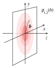
(a)	(b)

Figure 1: (a) Light–front view of a relativistic system. (b) Transverse densities in the nucleon. The function $\rho_{1}(b)$ describes the spin–independent part of the expectation value of the $J^{+}$ current in a nucleon state localized at the transverse origin, Eq. (25); the function $(2M_{N})^{-1}\,(b^{x}/b)\,\partial\rho_{2}(b)/\partial b$ the spin–dependent part in a nucleon polarized in the positive $y$–direction, Eq. (29).

The physical interpretation of the 2–dimensional densities refers to the light–front or partonic picture of nucleon structure and has been extensively discussed in the literature Soper:1976jc ; Burkardt:2000za ; Burkardt:2002hr ; Miller:2007uy ; Carlson:2007xd ; Miller:2010nz ; here we only summarize the main points. In the light–front picture one considers the evolution of a relativistic system in light–front time $x^{+}\equiv x^{0}+x^{3}=x^{0}+z$, as corresponds to clocks synchronized by a light–wave traveling through the system in the $z$–direction (see Fig. 1a). Particle states such as the nucleon are characterized by their light–cone momentum $p^{+}\equiv p^{0}+p^{z}$ and transverse momentum $\bm{p}_{T}\equiv(p^{x},p^{y})$, and $p^{-}\equiv p^{0}-p^{z}$ plays the role of the energy, with $p^{-}=(p_{T}^{2}+M_{N}^{2})/p^{+}$. One is generally interested in the “plus” component of the nucleon current, which possesses a simple interpretation in dynamical models. In a frame where the momentum transfer to the nucleon is in the transverse direction,

$$\Delta^{\pm}\;=\;0,\hskip 20.00003pt\bm{\Delta}_{T}\;=\;\bm{p}_{2T}-\bm{p}_{1T}\;\neq\;0,$$ (15)

the matrix element Eq. (1) takes the form

$$\langle p^{+},\bm{p}_{T2},\lambda_{2}|\,J^{+}(x)\,|p^{+},\bm{p}_{T1},\lambda_{1}\rangle\ = \bar{u}_{2}\left[\gamma^{+}F_{1}(t)\;+\;\frac{\sigma^{+i}\Delta_{T}^{i}}{2M_{N}}F_{2}(t)\right]u_{1}\,e^{-i\bm{\Delta}_{T}\bm{x}_{T}}$$ (16)

$$(t\;\equiv\;-\bm{\Delta}_{T}^{2}),$$

where now the momentum states are normalized as $\langle p_{2}^{+},\bm{p}_{T2}|p_{1}^{+},\bm{p}_{T1}\rangle=2p_{1}^{+}\,\delta(p_{2}^{+}-p_{1}^{+})\delta^{(2)}(\bm{p}_{T2}-\bm{p}_{T1})$. The polarization states of the initial and final nucleon can be defined in several ways and are usually chosen as helicity eigenstates, with $\lambda_{1,2}=\pm$ denoting the helicities. An explicit representation of the corresponding 4–spinors can be obtained by applying a Lorentz boost to rest–frame spinors polarized in the $z$–direction, and is given by Leutwyler:1977vy

$$u_{1}\;\;\equiv\;\;u(p^{+},\bm{p}_{1T},\lambda_{1})\;\;=\;\;\frac{\sqrt{2}}{\sqrt{p^{+}}}\left(p^{+}+\gamma^{0}M_{N}+\gamma^{0}\bm{\gamma}_{T}\bm{p}_{1T}\right)\frac{\gamma^{-}\gamma^{+}}{4}\left(\begin{array}[]{c}\chi(\lambda_{1})\\[4.30554pt] 0\end{array}\right),$$ (17)

and similarly for $u_{2}$. Here $\chi(\lambda=\pm)$ are rest frame 2–spinors for polarization in the positive and negative $z$–direction. The transition matrix element then falls into two structures, a “spin–independent” one proportional to

$$\delta({\lambda_{2},\lambda_{1}})\;\;=\;\;\chi^{\dagger}(\lambda_{2})\chi(\lambda_{1}),$$ (18)

which contains the Dirac form factor, and a “spin–dependent” one proportional to the vector

$$\bm{S}({\lambda_{2},\lambda_{1}})\;\;\equiv\;\;\chi^{\dagger}({\lambda_{2}})({\textstyle\frac{1}{2}}\bm{\sigma})\chi({\lambda_{1}}),$$ (19)

which contains the Pauli form factor.

To describe the transverse spatial structure of the nucleon one defines nucleon states in the transverse coordinate representation, corresponding to nucleons with a transverse center–of–momentum localized at given points $\bm{x}_{1T}$ and $\bm{x}_{2T}$, as

$$|\bm{x}_{1T}\rangle \equiv \int\frac{d^{2}p_{1T}}{(2\pi)^{2}}\;e^{-i\bm{p}_{1T}\bm{x}_{1T}}\;|\bm{p}_{1T}\rangle,$$ (20)

$$\langle\bm{x}_{2T}| \equiv \int\frac{d^{2}p_{2T}}{(2\pi)^{2}}\;e^{i\bm{p}_{2T}\bm{x}_{2T}}\;\langle\bm{p}_{2T}|,$$ (21)

which are normalized such that $\langle\bm{x}_{2T}|\bm{x}_{1T}\rangle=\delta^{(2)}(\bm{x}_{2T}-\bm{x}_{1T})$. We now consider the matrix element of the current at light–front time $x^{+}=0$ and position $x^{-}=0$, and a transverse position $\bm{x}_{T}$, between such transversely localized nucleon states with (arbitrary) longitudinal momentum $p^{+}$. Using Eqs. (16) and (17) it is straightforward to show that the spin–independent part of the matrix element of $J^{+}$ is given by

$$\langle p^{+},\bm{x}_{2T},\lambda_{2}|\;J^{+}(x^{\pm}=0,\bm{x}_{T})\;|p^{+},\bm{x}_{1T},\lambda_{1}\rangle_{\text{\scriptsize spin-indep.}}$$ (22)

$$= [2p^{+}\,\delta^{(2)}(\bm{x}_{2T}-\bm{x}_{1T})]\;\delta(\lambda_{2},\lambda_{1})\;\int\frac{d^{2}\Delta}{(2\pi)^{2}}\;e^{-i\bm{\Delta}_{T}(\bm{x}_{T}-\bm{x}_{1T})}\;F_{1}(-\bm{\Delta}_{T}^{2})$$

$$= [\ldots]\;\delta(\lambda_{2},\lambda_{1})\;\rho_{1}(\bm{x}_{T}-\bm{x}_{1T}).$$ (23)

The factor in brackets results from the normalization of the nucleon states. One sees that the function $\rho_{1}(b)$ of Eq. (10) describes the spin–independent part of the current in the nucleon, with

$$\bm{b}\;\;\equiv\;\;\bm{x}_{T}-\bm{x}_{1T}$$ (24)

defined as the displacement from the transverse center–of–momentum of the nucleon. In short, for a nucleon localized at the origin, $\bm{x}_{1T}=0$, the spin–independent current at transverse position $\bm{x}_{T}=\bm{b}$ is (see Fig. 1b)

$$\langle J^{+}(\bm{b})\rangle_{\text{\scriptsize spin-indep.}}\;\;=\;\;\rho_{1}(b).$$ (25)

Likewise, the spin–dependent part of the matrix element of $J^{+}$ is given by

$$\langle p^{+},\bm{x}_{2T},\lambda_{2}|\;J^{+}(x^{\pm}=0,\bm{x}_{T})\;|p^{+},\bm{x}_{1T},\lambda_{1}\rangle_{\text{\scriptsize spin-dep.}}$$ (26)

$$= [\ldots]\;(-i)\int\frac{d^{2}\Delta}{(2\pi)^{2}}\;e^{-i\bm{\Delta}_{T}(\bm{x}_{T}-\bm{x}_{1T})}\;\frac{\bm{S}(\lambda_{2},\lambda_{1})}{M_{N}}\cdot(\bm{e}_{z}\times\bm{\Delta}_{T})\;F_{2}(-\bm{\Delta}_{T}^{2})$$

$$= [\ldots]\;\frac{\bm{S}(\lambda_{2},\lambda_{1})}{M_{N}}\cdot\left(\bm{e}_{z}\times\frac{\partial}{\partial\bm{x}_{T}}\right)\;\rho_{2}(\bm{x}_{T}-\bm{x}_{1T}),$$ (27)

where $\bm{S}(\lambda_{2},\lambda_{1})$ is the spin vector of the transition defined in Eq. (19), and $\bm{e}_{z}$ the unit vector in the $z$–direction. Thus, the “crossed” gradient of the function $\rho_{2}(b)$ of Eq. (10) describes the spin–dependent current measured by an observer at a displacement $\bm{b}$ from the center–of–momentum of the nucleon. In Eq. (27) the nucleon polarization states are characterized by the $z$–component of the spin in the rest frame, $\lambda_{1,2}$, cf. Eq. (17). If instead we prepared initial and final nucleon state with definite spin in the $y$–direction and the same projection for both, the spin vector in Eq. (27) would be replaced by

$$\bm{S}(\lambda_{2},\lambda_{1})\;\;\rightarrow\;\;S^{y}\bm{e}_{y}\hskip 20.00003pt\text{(nucleon polarized in $y$--direction)},$$ (28)

where $S^{y}=\pm 1/2$ is the spin projection on the $y$–axis. For a nucleon localized at the origin and polarized in the $y$–direction, the spin–dependent current at a transverse position $\bm{b}$ is thus (see Fig. 1b)

$$\langle J^{+}(\bm{b})\rangle_{\text{\scriptsize spin-dep.}} = (2S^{y})\,\frac{\partial}{\partial b^{x}}\left[\frac{\rho_{2}(b)}{2M_{N}}\right]\;\;=\;\;(2S^{y})\,\frac{b^{x}}{b}\;\frac{\partial}{\partial b}\left[\frac{\rho_{2}(b)}{2M_{N}}\right]\;\;=\;\;(2S^{y})\,\cos\phi\;\widetilde{\rho}_{2}(b),$$ (29)

where $\cos\phi\equiv b^{x}/b$ is the cosine of the azimuthal angle and

$$\widetilde{\rho}_{2}(b) \equiv \frac{\partial}{\partial b}\left[\frac{\rho_{2}(b)}{2M_{N}}\right].$$ (30)

Now the term “spin–dependent” can be understood to mean that part of the current which changes sign when the transverse nucleon polarization is reversed. We shall refer to the function $\widetilde{\rho}_{2}$ as the “spin–dependent current density,” keeping in mind that the actual spin–dependent current matrix element involves also the polarization $(2S^{y})$ and the geometric factor $\cos\phi$. Note that for a given spin orientation the spin–dependent current changes sign between positive (“right,” when looking at the nucleon from $z=+\infty$) and negative (“left”) values of $b^{x}$, as would be the case for a convection current due to rotational motion around the $y$–axis. Finally, the total current in a nucleon polarized in the $y$–direction is then, in the same short–hand notation as used above,

$$\langle J^{+}(\bm{b})\rangle = \langle J^{+}(\bm{b})\rangle_{\text{\scriptsize spin-indep.}}\;+\;\langle J^{+}(\bm{b})\rangle_{\text{\scriptsize spin-dep.}}$$ (31)

$$= \rho_{1}(b)\;+\;(2S^{y})\;\cos\phi\;\widetilde{\rho}_{2}(b).$$ (32)

This expression, together with Eq. (30), concisely summarizes the physical significance of the transverse densities introduced as the 2–dimensional Fourier transforms of the invariant form factors, Eq. (10). We shall use it to develop a simple mechanical interpretation of the chiral component of the transverse densities below (see Sec. III.4).

The light–front interpretation of the nucleon current matrix elements described here assumes only that the momentum transfer to the nucleon is in the transverse direction, $\Delta^{\pm}=0$ and $\bm{\Delta}_{T}\neq 0$, but does not depend on the value of the nucleon’s longitudinal momentum $p^{+}$. As such it is valid for any $p^{+}$, including the rest frame where $p^{+}=M_{N}$. In Sec. III.4 we shall use the rest frame to obtain a simple interpretation of the relative order–of–magnitude of the chiral components of the charge and magnetization densities. Alternatively, one may consider the limit $p^{+}\rightarrow\infty$, where the description sketched here coincides with the conventional parton picture of nucleon structure (“infinite–momentum frame”).

In the present study we refer to the light–front representation of the transverse densities only for their interpretation; the actual calculations of the chiral component are carried out at the level the invariant form factors, without specifying a reference frame. For this purpose we may think of the transverse densities defined by Eq. (10) as just a particular functional transform of the invariant form factors, i.e., an equivalent mathematical representation of the information contained in these functions. We shall return to the light–front picture only at the end, when interpreting the results of our calculation. The power of transverse densities is precisely that they connect the invariant form factors with the light–front picture of nucleon structure and can be accessed from both sides.

In dynamical models where the nucleon has a composite structure, the transverse densities Eq. (10) can be represented as overlap integrals of the frame–independent light–cone wave functions of the system. With the momentum transfer chosen such that $\Delta^{\pm}=0$ and $\bm{\Delta}_{T}\neq 0$ the current cannot produce particles but simply “counts” the charge and current of the constituents in the various configuration of the wave functions. It is possible to compute the chiral component of transverse densities directly in this formulation, using light–front time–ordered perturbation theory; this approach will be explored in a subsequent article inprep .

II.2 Dispersion representation

Much insight into the behavior of the transverse densities can be gained by making use of the analytic properties of the nucleon form factors as functions of the invariant momentum transfer. The form factors $F_{1,2}(t)$ are analytic functions of $t$, with singularities (branch cuts, poles) on the positive real axis. They correspond to processes in which a current with timelike momentum converts to a hadronic state coupling to the nucleon, which may occur below the physical threshold for nucleon–antinucleon ($N\bar{N}$) pair production. The principal cut in the physical sheet of the form factor starts at the squared mass of the lowest hadronic state, the two–pion state, $t=4M_{\pi}^{2}$, and runs to $t=+\infty$. Assuming that the form factors vanish at $|t|\rightarrow\infty$, as expected from the power behavior implied by perturbative QCD (with logarithmic modifications) and supported by present experimental data, the form factors satisfy an unsubtracted dispersion relation,

$$F_{1,2}(t)\;\;=\;\;\int\limits_{4M_{\pi}^{2}}^{\infty}\frac{dt^{\prime}}{t^{\prime}-t}\;\frac{\textrm{Im}\,F_{1,2}(t^{\prime}+i0)}{\pi}.$$ (33)

It expresses the form factors as integrals over their imaginary parts on the principal cut, also known as the spectral functions. In the region below the $N\bar{N}$ threshold, $t^{\prime}<4M_{N}^{2}$, which dominates the integral Eq. (33) at all values of $t$ of interest, the spectral function cannot be measured directly in conversion experiments and can only be calculated using theoretical methods (dispersion theory, chiral EFT) or determined empirically from fits to form factor data Hohler:1976ax ; Belushkin:2006qa . Even so, this representation of the form factor turns out to be extremely useful for the theoretical analysis of transverse densities. Substituting Eq. (33) in Eq. (13) and carrying out the Fourier integral, one obtains a dispersion (or spectral) representation of the transverse densities of the form Strikman:2010pu

$$\rho_{1,2}(b)\;\;=\;\;\int\limits_{4M_{\pi}^{2}}^{\infty}\frac{dt}{2\pi}\;K_{0}(\sqrt{t}b)\;\frac{\textrm{Im}\,F_{1,2}(t+i0)}{\pi},$$ (34)

where $K_{0}$ denotes the modified Bessel function and we have dropped the prime on the integration variable $t$. This representation has several interesting mathematical properties. Because of the exponential decay of the modified Bessel function at large arguments,

$$K_{0}(\sqrt{t}b)\;\;\sim\;\;\sqrt{\frac{\pi}{2}}\;\frac{e^{-\sqrt{t}b}}{(\sqrt{t}b)^{1/2}}\hskip 20.00003pt(\sqrt{t}b\;\gg\;1),$$ (35)

the dispersion integral for the density converges exponentially at large $t$, in contrast to the power–like convergence of the original integral for the form factor, Eq.(33) . Equation (34) thus corresponds to integrating over the spectral function with an exponential filter of width $1/b$ applied to the energy $\sqrt{t}$. Significant numerical suppression happens already inside the range $\sqrt{t}\lesssim 1/b$ and determines the absolute magnitude of the resulting density; the important point is that the contribution from larger energies in the integral are relatively suppressed compared to those inside the range with exponential strength (see Refs. Miller:2010tz ; Miller:2011du for a detailed discussion). In this sense the transverse distance $b$ acts as an external parameter that allows one to “select” energies in the range $\sqrt{t}\lesssim 1/b$ in the spectral functions of the form factors.

The spectral representation Eq. (34) is particularly suited to the study of the asymptotic behavior of the transverse densities at large distances. Generally, any singularity (pole or branch cut) in the form factors at a squared mass $t=\mu^{2}$, which contributes to the imaginary parts $\textrm{Im}\,F_{1,2}(t+i0)$, produces densities which asymptotically decay as

$$\rho_{1,2}(b)_{\text{singularity at}\;\mu^{2}}\;\;\sim\;\;P_{1,2}(b)\;e^{-\mu b}\hskip 20.00003pt(b\rightarrow\infty),$$ (36)

where $P_{1,2}$ are functions with power–like asymptotic behavior. The rate of exponential decay is governed by the position of the singularity alone; the pre-exponential factor $P_{1,2}$ depends on the strength of the singularity and the variation of the spectral functions over the relevant range of integration (which may involve other mass scales besides $\mu$) and has to be determined by detailed calculation. Equation (36) expresses the traditional notion of the range of an “exchange mechanism” in the spatial representation of nucleon structure through transverse densities.

Here we are interested in the transverse densities in the chiral periphery, at distances of the order $b\sim M_{\pi}^{-1}$. In the context of the spectral representation Eq. (34) the densities at such distances are determined by the behavior of the spectral function near the two–pion threshold, $t=4M_{\pi}^{2}$; more precisely, at masses

$$t-4M_{\pi}^{2}\;\;\sim\;\;\textrm{few}\;M_{\pi}^{2}.$$ (37)

Physically, this corresponds to chiral processes in which the current operator couples to the nucleon by exchange of two “soft” pions, with momenta $|\bm{k}_{1,2}|\sim\textrm{few}\,M_{\pi}$ in the nucleon rest frame (details will be given below). The two–pion cut in the nucleon form factor has isovector quantum numbers and contributes with different sign to the proton and neutron. In our theoretical analysis we therefore focus on the isovector combination of the form factors and the transverse densities,

$$\rho^{V}(b)\;\;\equiv\;\;{\textstyle\frac{1}{2}}[\rho^{p}(b)-\rho^{n}(b)].$$ (38)

In the isoscalar density the chiral contribution starts with three–pion exchange and is numerically irrelevant at all distances of interest (see Refs. Miller:2011du for a phenomenological analysis).

The spectral representation of Eq. (34) offers many practical advantages for the study of the chiral component of the transverse densities. First, it relates the chiral component to the isovector spectral function near threshold, which possesses a rich structure (see Sec. II.3) that expresses itself in the densities and can be exhibited in this way. The calculation of the spectral function in chiral EFT is particularly simple and can be performed very efficiently using $t$–channel cutting rules. The chiral and heavy–baryon expansions of the spectral functions have been studied extensively in the literature Gasser:1987rb ; Bernard:1996cc ; Becher:1999he ; Kubis:2000zd ; Kaiser:2003qp , and these results can directly be imported into the study of transverse densities. Second, the spectral representation allows us to combine chiral and non–chiral contributions to the transverse densities in a consistent manner. The latter arise from higher–mass states in the spectral functions, particularly the $\rho$ meson in the isovector channel. The total spectral function can be constructed such that the chiral EFT result is used only in the near–threshold region $t-4M_{\pi}^{2}\sim\textrm{few}\;M_{\pi}^{2}$, where the chiral expansion is manifestly valid, and the higher–mass region is parametrized empirically. In this way the chiral and non–chiral components can be added without double–counting and compared quantitatively as functions of $b$.

In the following we use the the spectral representation Eq. (34) as a tool to calculate the chiral component of the transverse densities in chiral EFT. It is worth noting that this representation has many applications beyond this specific purpose. It can be used to quantify the vector meson contribution in the nucleon’s transverse densities Miller:2011du , and to construct the transverse charge density in the pion from precise data of the timelike form factor obtained in $e^{+}e^{-}$ annihilation experiments Miller:2010tz . It can also be extended to other nucleon form factors and corresponding densities, such as the form factors of the energy–momentum tensor and the “generalized form factors” defined by the moments of the nucleon GPDs.

II.3 Spectral functions near threshold

The isovector transverse densities in the chiral periphery are determined by the spectral functions of the nucleon form factors in the vicinity of the two–pion threshold at $t=4M_{\pi}^{2}$. Before turning to the chiral EFT calculations it is worth reviewing the analytic structure of the form factor near threshold as it follows from general considerations Frazer:1960zza ; Frazer:1960zzb ; Hohler:1976ax . In particular, this explains the nature of the subthreshold singularity at $t=4M_{\pi}^{2}-M_{\pi}^{4}/M_{N}^{2}$, which defines the parametric regimes in the analysis of the transverse densities and determines the convergence of the chiral expansion.

The spectral functions at $t=4M_{\pi}^{2}+\textrm{few}\,M_{\pi}^{2}$ result from virtual processes in which the current couples to the nucleon by conversion to a two–pion state of mass $\sqrt{t}$ (see Fig. 2a). The coupling of this system to the nucleon is described by the $\pi N$ scattering amplitude, which at $t<0$ can be determined in $\pi N$ scattering experiments but is evaluated here in the region $t>0$. The analytic structure of the $\pi N$ scattering amplitude implies the existence of certain singularities on the unphysical sheet of the nucleon form factor, below the principal cut starting at $t=4M_{\pi}^{2}$ (see Fig. 2b). They occur because for certain values of $t$ the invariant mass of the $s$–channel intermediate state of the $\pi N$ scattering process can reach the value of physical baryon masses (specifically, the $N$ and $\Delta$), where the $\pi N$ scattering amplitude has a pole. This can be seen most easily in the center–of–mass frame of the $t$–channel process of production of the two–pion system by the electromagnetic current. Let $p_{1,2}$ be the 4–momenta of the initial and final nucleon, and $k_{1,2}$ those of the two pions. Introducing the average nucleon and pion 4–momenta and their difference,

$$P\;\equiv\;{\textstyle\frac{1}{2}}(p_{1}+p_{2}),\hskip 20.00003ptk\;\equiv\;{\textstyle\frac{1}{2}}(k_{1}+k_{2}),\hskip 20.00003pt\Delta\;\equiv\;p_{2}-p_{1}\;=\;k_{2}-k_{1},$$ (39)

we express the individual 4–momenta as $p_{1,2}=P\mp\Delta/2$ and $k_{1,2}=k\mp\Delta/2$. The mass shell conditions for the initial and final nucleon 4–momenta imply

$$P\Delta = 0,$$ (40)

$$P^{2} = M_{N}^{2}-t/4,$$ (41)

where $t=\Delta^{2}$.

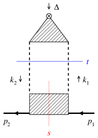
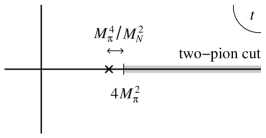
(a)	(b)

Figure 2: (a) Virtual processes generating the two–pion cut in the nucleon form factor. The triangle denotes the timelike pion form factor, the rectangle the full $\pi N$ scattering amplitude in the region $t>4M_{\pi}^{2}$. (b) Analytic structure of the nucleon form factor in the vicinity of the two–pion threshold $t=4M_{\pi}^{2}$. The cross denotes the subthreshold singularity on the unphysical sheet, resulting from the intermediate nucleon pole in the $\pi N$ amplitude in the virtual process [see drawing (a)].

The spectral function corresponds to the process of Fig. 2a with on–shell external nucleons but values of $t>4M_{\pi}^{2}$, for which the current can produce a two–pion state. In this state also the pion 4–momenta are on mass–shell, and in addition to Eq. (40) and (41) one has the relations

$$k\Delta = 0,$$ (42)

$$k^{2} = M_{\pi}^{2}-t/4.$$ (43)

The $t$–channel center–of–mass (or CM) frame is defined as the frame in which the 4–momentum of the current, which is the total 4–momentum of the pion pair, has components

$$\Delta^{\mu}\;\;=\;\;(\sqrt{t},0,0,0),$$ (44)

where $t>0$. Because of Eq. (40) the average nucleon momentum $P$ in this frame has only spatial components, and we choose it to point in the $z$–direction,

$$P^{\mu}\;\;=\;\;\left(0,0,0,P^{z}\right),$$ (45)

where the component $P^{z}$ is determined by Eq. (41) as

$$P^{z}\;\;=\;\;\left\{\begin{array}[]{lll}{\textstyle\sqrt{t/4-M_{N}^{2}}}&=\sqrt{-P^{2}}&t>4M_{N}^{2},\\[4.30554pt] i\textstyle{\sqrt{M_{N}^{2}-t/4}}&=i\sqrt{P^{2}}&t<4M_{N}^{2}.\end{array}\right.$$ (46)

In the near–threshold region $t=4M_{\pi}^{2}+\textrm{few}\,M_{\pi}^{2}$ we need to use the lower expression, where the value of $P^{z}$ is imaginary. Note that the sign of the imaginary part of $P^{z}$ in the region $t<4M_{N}^{2}$ follows from the analytic continuation of the expression for $t>4M_{N}^{2}$ with the prescription $t\rightarrow t+i0$. In sum, the choice of 4–vectors Eqs. (44)–(46) satisfies the invariant constraints Eqs. (40)–(41) for any value of $t>0$.

Further in the CM frame, Eq. (42) requires that the average pion 4–momentum $k$ have components

$$k^{\mu}\;=\;\left(0,\bm{k}\right),$$ (47)

and the modulus of the 3–momentum is determined by Eq. (43) as

$$|\bm{k}|\;=\;{\textstyle\sqrt{t/4-M_{\pi}^{2}}}\;\equiv\;\;k_{\rm cm}$$ (48)

and referred to as the pion CM momentum. Here we assume that $t>4M_{\pi}^{2}$; the values of $k_{\rm cm}$ below threshold are obtained by analytic continuation with $t\rightarrow t+i0$. Denoting the polar angle of the pion momentum by $\theta$, we have

$$k^{z}\;=\;k_{\rm cm}\,\cos\theta,\hskip 20.00003ptkP\;=\;-ik_{\rm cm}\sqrt{P^{2}}\cos\theta.$$ (49)

The two–pion contribution to the spectral functions of the electromagnetic form factors at $t>4M_{\pi}^{2}$ is now given by the product of the invariant amplitudes for the $\textrm{current}\rightarrow\pi\pi$ and the $\pi\pi\rightarrow N\bar{N}$ transitions, integrated over the solid angle of the pion CM momentum $\bm{k}$ (Fig. 2a). Because of $t$–channel angular momentum conservation the angular dependence of the $\textrm{current}\rightarrow\pi\pi$ amplitude in the CM frame is $\sim\cos\theta$, and the integral projects the $\pi\pi\rightarrow N\bar{N}$ amplitude on the $J=1$ partial wave (P wave). The well–known result is Frazer:1960zza ; Frazer:1960zzb ; Hohler:1976ax

$$\frac{1}{\pi}\textrm{Im}\,F_{1,2}(t)\;\;=\;\;\frac{k_{\rm cm}^{3}}{\pi\sqrt{t}}\;F_{\pi}^{\ast}(t)\;\Gamma_{1,2}(t),$$ (50)

where $F_{\pi}^{\ast}(t)$ is the (complex–conjugate) pion form factor and $\Gamma_{1,2}(t)$ the $\pi\pi\rightarrow N\bar{N}$ partial wave amplitude Hohler:1974ht .

Equation (50) describes the spectral functions of the form factors, which are real functions defined in the physical region of the $t$–channel process, $t>4M_{\pi}^{2}$. The behavior of the complex form factors themselves can be studied in a very similar manner, by interpreting Eq. (50) as a discontinuity of the complex function which can be analytically continued. The net result is that the singularities of the $\pi\pi\rightarrow N\bar{N}$ partial–wave amplitude are “transmitted” to the form factors Frazer:1960zza ; Frazer:1960zzb ; Hohler:1976ax . Specifically, at a given value of $t$ and $\cos\theta$, the squared invariant mass of the $s$–channel intermediate state in the $\pi N$ invariant amplitude is (see Fig. 2a)

$$s \equiv (p_{1}-k_{1})^{2}\;\;=\;\;(p_{2}-k_{2})^{2}\;\;=\;\;(k-P)^{2}$$ (51)

$$= -k_{\rm cm}^{2}-t/4+2ik_{\rm cm}\sqrt{P^{2}}\cos\theta+M_{N}^{2}.$$

The $\pi N$ invariant amplitude has singularities at the values of $s$ corresponding to physical intermediate states; in particular the nucleon pole at $s=M_{N}^{2}$. Upon integration over $\cos\theta$, it produces branch cut singularities in the partial wave amplitudes $\Gamma_{1,2}(t)$ on the unphysical sheet of $t$. The start of the cut (the position of the branch point) coincides with the end points of the angular integration and is thus determined by the condition $s(t,\cos\theta=\pm 1)=M_{N}^{2}$, or

$$-k_{\rm cm}^{2}-t/4\;\;=\;\;\pm 2ik_{\rm cm}\sqrt{P^{2}}.$$ (52)

Taking the square of both sides, and substituting the expressions Eqs. (41) and (48) for $P^{2}$ and $k_{\rm cm}$, this becomes

$$(t/2-M_{\pi}^{2})^{2}\;\;=\;\;-(t-4M_{\pi}^{2})(M_{N}^{2}-t/4),$$ (53)

the solution of which is

$$t\;\;=\;\;4M_{\pi}^{2}\;-\;\frac{M_{\pi}^{4}}{M_{N}^{2}}\;\;\equiv\;\;t_{\rm sub}.$$ (54)

In sum, the form factors as analytic functions of $t$ have a branch cut on the unphysical sheet, starting at the value given by Eq. (54), which corresponds to the intermediate nucleon state in the $\pi N$ scattering amplitude going on mass shell (see Fig. 2b) Frazer:1960zza ; Frazer:1960zzb ; Hohler:1976ax . The presence of this subthreshold singularity can be established on general grounds; it can also be seen explicitly in the relativistic chiral EFT results quoted below.

A point of great importance is that the distance of the subthreshold singularity from the threshold is small on the scale of $M_{\pi}^{2}$:

$$t_{\rm sub}\;-\;4M_{\pi}^{2}\;\;=\;\;\epsilon^{2}\,M_{\pi}^{2},$$ (55)

where

$$\epsilon\;\;\equiv\;\;\frac{M_{\pi}}{M_{N}}.$$ (56)

The ratio $\epsilon$ is a small parameter in both the chiral and the heavy–baryon limit. The spectral functions of the isovector form factors thus exhibit structure on two different scales. Looking at them on the “coarse” scale, $t=O(M_{\pi}^{2})$, one sees them rising from the threshold at $t=4M_{\pi}^{2}$ and varying on average with a characteristic scale $\sim M_{\pi}^{2}$. Looking at the functions near threshold on the “fine” scale, $t-4M_{\pi}^{2}=O(\epsilon^{2}M_{\pi}^{2})$, one sees a variation with characteristic scale $\epsilon^{2}M_{\pi}^{2}$, caused by the closeness of the subthreshold singularity.

The presence of a singularity close to the physical threshold affects the convergence of the chiral expansion of the spectral function near threshold Bernard:1996cc ; Becher:1999he ; Kubis:2000zd ; Kaiser:2003qp . For instance, one immediately sees that a naive expansion of $\textrm{Im}\,F_{1,2}(t)$ in powers of the pion CM momentum $k_{\rm cm}$ would converge only in the parametrically small region $t-4M_{\pi}^{2}<\epsilon^{2}$, or $k_{\rm cm}<\epsilon/2$, and thus produce unnaturally large expansion coefficients growing like inverse powers of $\epsilon$. This situation generally requires the use of different expansion schemes in different parametric regions of $t$; uniform approximations can be obtained by matching the different expansions Becher:1999he .

The nucleon pole in the $\pi N$ scattering amplitude is special in that it produces a subthreshold singularity extremely close to the threshold, which strongly influences the behavior of the spectral function above threshold. Higher mass $\pi N$ resonances give rise to further subthreshold singularities of the form factor, which, however, lie farther away from threshold. Below we consider the $\Delta$ isobar at $M_{\Delta}=1.23\,\textrm{GeV}$, which couples strongly to the $\pi N$ channel and becomes degenerate with the $N$ in the large–$N_{c}$ limit of QCD. For this state the pole condition $s=M_{\Delta}^{2}$ becomes [cf. Eq. (52)]

$$-k_{\rm cm}^{2}-t/4-M_{\Delta}^{2}+M_{N}^{2}\;\;=\;\;\pm 2ik_{\rm cm}\sqrt{P^{2}},$$ (57)

whose solution is

$$t\;\;=\;\;4M_{\pi}^{2}-\frac{(M_{\Delta}^{2}-M_{N}^{2}+M_{\pi}^{2})^{2}}{M_{\Delta}^{2}}\;\;\equiv\;\;t_{{\rm sub},\Delta}$$ (58)

[the expression reduces to Eq. (54) if one sets $M_{\Delta}=M_{N}$]. One sees that this subthreshold singularity is removed from threshold by a distance in $t$ that does not tend to zero in the chiral limit $M_{\pi}\rightarrow 0$. Numerically, with the physical $\pi,N$ and $\Delta$ masses, the distance from threshold is $0.022\,M_{\pi}^{2}$ for the $N$ and $0.43\,M_{\pi}^{2}$ (or 20 times larger) for the $\Delta$ singularity, showing clearly the qualitative difference between the $N$ pole and higher–mass $\pi N$ resonances.

II.4 Parametric regions of transverse distance

In the context of our dispersion analysis of transverse densities, the “two–scale” structure of the spectral function near threshold defines the parametric regions of the transverse distance $b$ at which we aim to compute the densities. Again, it is useful to establish this connection on general grounds, before turning to the actual chiral expansion of the functions.

In the dispersion integral Eq. (34) the distance $b$ effectively controls the region of $t$–channel masses over which the spectral function is integrated. To make this more explicit, we substitute the asymptotic expression Eq. (35) for the modified Bessel function; the deviations between the exact function and the asymptotic approximation are not important for the parametric estimates made here. We obtain

$$\rho_{1,2}(b)\;\;=\;\;e^{-2M_{\pi}b}\;\int\limits_{4M_{\pi}^{2}}^{\infty}dt\;\frac{e^{-(\sqrt{t}-2M_{\pi})b}}{(8\pi\sqrt{t}b)^{1/2}}\;\frac{\textrm{Im}\,F_{1,2}(t+i0)}{\pi}.$$ (59)

We have extracted the exponential factor $\exp(-2M_{\pi}b)$ from the integral, so that the remaining integral represents the pre-exponential factor $P_{1,2}(b)$ in the general asymptotic form Eq. (36). In Eq. (59) the exponential function under the integral restricts the integration to masses $\sqrt{t}$ for which

$$(\sqrt{t}-2M_{\pi})b\;\;=\;\;O(1).$$ (60)

We can therefore distinguish two parametric regions in $b$.

• In the region

  $$b\;=\;O(M_{\pi}^{-1})\hskip 20.00003pt\textrm{(``chiral distances'')}$$ (61)

  the integral of Eq. (59) extends over masses in the region

  $$\sqrt{t}-2M_{\pi}\;=\;O(M_{\pi}),\hskip 20.00003pt\textrm{or}\hskip 20.00003ptt-4M_{\pi}^{2}\;=\;O(M_{\pi}^{2}),$$ (62)

  with no additional restriction to values near threshold. The $t$–channel pion CM momenta are of the order

  $$k_{\rm cm}\;=\;O(M_{\pi}),$$ (63)

  which is the domain usually associated with chiral dynamics.

• In the region

  $$b\;=\;O(\epsilon^{-2}M_{\pi}^{-1})\;=\;O(M_{N}^{2}/M_{\pi}^{3})\hskip 20.00003pt\textrm{(``molecular distances'')}$$ (64)

  [$\epsilon=M_{\pi}/M_{N}$, cf. Eq. (56)] the integral over masses is restricted to the near–threshold region

  $$\sqrt{t}-2M_{\pi}\;=\;O(\epsilon^{2}M_{\pi}),\hskip 20.00003pt\textrm{or}\hskip 20.00003ptt-4M_{\pi}^{2}\;=\;O(\epsilon^{2}M_{\pi}^{2}).$$ (65)

  The distance of $t$ from threshold is comparable to that of the subthreshold singularity from threshold, Eq. (55), so that the behavior of the spectral function is essentially influenced by the subthreshold singularity. The pion CM momenta are now of the order

  $$k_{\rm cm}\;=\;O(\epsilon M_{\pi}),$$ (66)

  corresponding to the $t$–channel system moving non–relativistically with velocity $v=k_{\rm cm}/M_{\pi}=O(\epsilon)$.

We refer to the parametric domain of Eq. (64) as the molecular region, as the typical transverse distances between the pion and the initial/final nucleon are much larger than the Compton wavelength of the pion. At the physical pion and nucleon mass $\epsilon\approx 1/7$, so that such distances can numerically be as large as $10^{2}\,\textrm{fm}$. Since the densities decay with an overall exponential factor of $\exp(-2M_{\pi}b)$, they are extremely small at such large distances. The molecular region of the nucleon’s transverse densities is therefore mostly of theoretical interest. However, the existence of this regime in coordinate space affects the magnitude of higher $b^{2}$–weighted moments of the densities, which are proportional to higher derivatives of the form factors at $t=0$, and thus may in principle have observable consequences.

The parametric classification of distances, Eqs. (61) and Eqs. (64), can be established on general grounds, starting from the scales governing the behavior of the spectral function. In Sec. III.3 we show that the invariant chiral EFT result bears out this general structure and perform the heavy–mass expansion of the densities in the different parametric regions. We note that the existence of a regime of anomalously large distances $\sim M_{N}^{2}/M_{\pi}^{3}$ is not specific to the isovector transverse charge and magnetization densities but common to all nucleon observables governed by $t$–channel exchange of two pions, which are sensitive to the subthreshold singularities of the $\pi N$ scattering amplitude. A similar phenomenon has been observed in the two–pion exchange contribution to the low–energy $NN$ interaction, where it can be expressed in terms of the large–distance behavior of the 3–dimensional $NN$ potential Robilotta:1996ji ; Robilotta:2000py ; see Ref. Epelbaum:2005pn for a review.

III Peripheral densities from chiral dynamics

III.1 Two–pion spectral functions

We now want to calculate the chiral component of the transverse densities in the nucleon within the framework laid out in Sec. I. We use the leading–order chiral EFT results for the spectral functions of the form factors to compute the peripheral densities from the dispersion integral Eq. (59) and study their properties in the parametric regions identified in Sec. II.4. In view of the essential role of analyticity we employ the relativistic formulation of chiral EFT with baryons, which generates amplitudes with the correct analytic structure in the form of Feynman diagrams with relativistic propagators; the heavy–baryon limit will be investigated by expanding the explicit expressions obtained in the relativistic formulation.

The spectral functions of the nucleon form factors have been studied extensively both in the relativistic and the heavy–baryon formulations of chiral EFT Gasser:1987rb ; Bernard:1996cc ; Becher:1999he ; Kubis:2000zd ; Kaiser:2003qp (see e.g. Ref. Kaiser:2003qp for a discussion of the literature), and we can use these results for our purposes. For several reasons it will be useful to revisit the leading–order relativistic calculation and summarize the essential steps here. First, the spectral functions can be computed very efficiently using $t$–channel cutting rules; this method can easily be extended to $\Delta$ intermediate states (see Sec. IV) and to form factors of other operators (energy–momentum tensor, GPD moments) that will be calculated in a future study. Second, we need the explicit expressions of the Feynman integrals for the partonic interpretation of our results and future comparison with the light–front approach. In particular, the physical origin of the contact term in the chiral EFT result for the spectral function of $F_{1}$ is best understood at the level of the original Feynman integrals and was not discussed in this form before. Third, we present a very compact representation of the leading–order chiral EFT results that can easily be used for numerical analysis.

In the relativistic formulation of chiral EFT with nucleons Becher:1999he the leading–order chiral Lagrangian is given by $\mathcal{L}^{(1)}_{\chi}=\mathcal{L}^{(1)}_{N}+\mathcal{L}^{(1)}_{\pi}$, where $\mathcal{L}^{(1)}_{\pi}$ is the usual chiral Lagrangian of the pion field, while $\mathcal{L}^{(1)}_{N}$ describes the dynamics of the nucleon field and its coupling to the pion and is of the form

$$\mathcal{L}^{(1)}_{N} = \bar{\psi}[i(\hat{\partial}+\hat{\Gamma})-M_{N}]\psi\;+\;{\textstyle\frac{1}{2}}g_{A}\bar{\psi}\hat{u}\gamma_{5}\psi.$$ (67)

$$\Gamma_{\mu} \equiv {\textstyle\frac{1}{2}}[U^{-1/2},\partial_{\mu}(U^{1/2})],$$ (68)

$$u_{\mu} \equiv i\,U^{-1/2}\,(\partial_{\mu}U)\,U^{-1/2},$$ (69)

$$U \equiv \exp[i\bm{\pi}\cdot\bm{\tau}/{F_{\pi}}],\hskip 20.00003ptU^{\pm 1/2}\;=\;\exp[\pm i\bm{\pi}\cdot\bm{\tau}/(2F_{\pi})],$$ (70)

where $\hat{\partial}\equiv\partial_{\mu}\gamma^{\mu}$ etc. Here $\psi$ is the Dirac field of the nucleon, and $\pi^{a}(a=1,2,3)$ the chiral pion field. In Eq. (67) $g_{A}$ denotes the nucleon axial vector coupling and $F_{\pi}$ the pion decay constant; at leading order these parameters are taken at their physical (tree–level) values $g_{A}=1.26$ and $F_{\pi}=93\,\textrm{MeV}$. In the calculation of the leading–order isovector spectral functions one needs the pion–nucleon coupling to second order in the pion field. Expanding Eq. (67) in powers of the pion field one obtains

$$\mathcal{L}^{(1)}_{N} = \bar{\psi}(i\hat{\partial}-M_{N})\psi\;-\;\frac{g_{A}}{2F_{\pi}}\bar{\psi}\gamma_{\mu}\gamma_{5}\tau^{a}\psi\;\partial_{\mu}\pi^{a}\;-\;\frac{1}{4F_{\pi}^{2}}\bar{\psi}\gamma_{\mu}\tau^{a}\psi\;\epsilon^{abc}\pi^{b}\partial_{\mu}\pi^{c}.$$ (71)

The second term on the right–hand side of Eq. (71) describes a Yukawa–type $\pi NN$ coupling (three–point vertex). We note that the axial vector coupling used here is equivalent to the conventional pseudoscalar $\pi NN$ coupling for on–shell nucleons; namely

$$-\frac{g_{A}}{2F_{\pi}}\bar{u}_{2}i\hat{\Delta}\gamma_{5}\tau^{a}u_{1} = \frac{g_{A}M_{N}}{F_{\pi}}\bar{u}_{2}i\gamma_{5}\tau^{a}u_{1}\;\;\equiv\;\;g_{\pi NN}\bar{u}_{2}i\gamma_{5}\tau^{a}u_{1}$$ (72)

between nucleon spinors $u_{1}\equiv u(p_{1})$ and $\bar{u}_{2}\equiv\bar{u}(p_{2})$ with $\Delta=p_{2}-p_{1}$. The identification of the pseudoscalar coupling constant of Eq. (72) is precisely the Goldberger–Treiman relation for the nucleon’s axial current matrix element. The third term in Eq. (71) describes a local $\pi\pi NN$ coupling (four–point vertex). Its appearance is due to the specific representation of the nucleon fields adopted in Eq. (67), and the coupling constant is fixed by chiral symmetry and does not involve any free parameter. The vertex couples the isovector–vector current of the nucleon field to that of the pion field.

Figure 3: The Feynman diagrams describing the leading–order chiral contributions to the two–pion cut of the isovector nucleon form factor. The dotted line indicates the Cutkosky cut.

The calculation of the spectral functions starts from the matrix element of the electromagnetic current between nucleon states. In general the electromagnetic current operator of the effective chiral theory consists of the currents of the pion and nucleon fields and contributions resulting from their pointlike interactions. We are interested only in the spectral functions of the isovector form factors in the region $t=4M_{\pi}^{2}+\textrm{few}\;M_{\pi}^{2}$, which results from processes in which the current couples to the nucleon through two–pion exchange. In leading order these are given by the two Feynman diagrams of Fig. 3, where the current is the leading–order isovector current of the pion field,

$$J_{\pi}^{\mu,\,(1)}\;\;=\;\;\epsilon^{3ab}\pi^{a}\partial^{\mu}\pi^{b}.$$ (73)

Other diagrams appearing at the same order only contribute to the two–nucleon cut of the spectral function [which gives a short–distance contribution to the density at $b=O(M_{N}^{-1})$] or modify the real part of the nucleon vertex function current, but do not contribute to the two–pion cut; this simplification is a major advantage of the dispersive approach. The contributions to the isovector current matrix element resulting from the diagrams of Fig. 3 can be computed using standard rules of Lorentz–invariant perturbation theory, and one obtains

$$\langle N_{2}|\,J^{\mu}(0)\,|N_{1}\rangle_{\pi\pi\;{\rm cut}} = \frac{ig_{A}^{2}}{F_{\pi}^{2}}\;\int\!\frac{d^{4}k}{(2\pi)^{4}}\;\;\frac{[\bar{u}_{2}\hat{k}_{2}\gamma_{5}(\hat{l}+M_{N})\hat{k}_{1}\gamma_{5}u_{1}]\,k^{\mu}}{(k_{1}^{2}-M_{\pi}^{2}+i0)(k_{2}^{2}-M_{\pi}^{2}+i0)(l^{2}-M_{N}^{2}+i0)}$$ (74)

$$+ \frac{i}{F_{\pi}^{2}}\;\int\!\frac{d^{4}k}{(2\pi)^{4}}\;\frac{(\bar{u}_{2}\hat{k}u_{1})\,k^{\mu}}{(k_{1}^{2}-M_{\pi}^{2}+i0)(k_{2}^{2}-M_{\pi}^{2}+i0)}.$$ (75)

The label “$\pi\pi$ cut” indicates that we retain only the diagrams contributing to the two–pion cut. The first integral, Eq. (74), results from diagram Fig. 3a with the $\pi NN$ three–point vertex; the second, Eq. (75), from diagram Fig. 3b with the $\pi\pi NN$ four–point vertex (or contact term). In both diagrams the pion 4–momenta are decomposed as

$$k_{1,2}\;\;=\;\;k\mp\Delta/2,$$ (76)

and the average momentum $k$ was chosen as integration variable. In Eq. (75) we have dropped terms in the integrand which integrate to zero because of the symmetry of the integrand with respect to reflections $k\rightarrow-k$. In Eq. (74)

$$l \equiv p_{1}-k_{1}\;\;=\;\;p_{2}-k_{2}\;\;=\;\;P-k$$ (77)

is the 4–momentum of the intermediate nucleon, with $P=(p_{1}+p_{2})/2$ the average nucleon momentum. The expression of this diagram can be simplified further. Namely, the integral in Eq. (74) contains a term in which the pole of the intermediate nucleon propagator cancels, and which is of the same structure as the integral of Eq. (75). Making use of the anticommutation relations between the gamma matrices and the Dirac equation for the nucleon spinors, one can rewrite the bilinear form in Eq. (74) as

$$\bar{u}_{2}\hat{k}_{2}\gamma_{5}(\hat{l}+M_{N})\hat{k}_{1}\gamma_{5}u_{1} = \bar{u}_{2}\left[-2M_{N}(l^{2}-M_{N}^{2})-(l^{2}-M_{N}^{2})\hat{k}-4M_{N}^{2}\hat{k}\right]u_{1}.$$ (78)

The first term in the bracket on the right–hand side integrates to zero because the integrand is antisymmetric under $k\rightarrow-k$, and can be dropped. The second term leads to an integral of the same form as Eq. (75) and can be combined with Eq. (75), effectively changing the coefficient of the contact term resulting from diagram Fig. 3b as

$$\frac{1}{F_{\pi}^{2}}\;\;\rightarrow\;\;\frac{1-g_{A}^{2}}{F_{\pi}^{2}}.$$ (79)

The appearance of the combination $1-g_{A}^{2}$ here is not accidental but has a deeper physical meaning, as is explained in Sec. III.5. The third term in Eq. (78) represents the genuine “non–contact” contribution from the diagram Fig. 3a, corresponding to an intermediate state with a propagating nucleon.

The tensor integrals in Eq. (74) and (75) can be reduced to scalar integrals with the help of standard projection formulas. Using the Dirac equation to convert the resulting bilinear forms $\bar{u}_{2}\ldots u_{1}$ to those of the right–hand side of Eq. (1), one obtains the chiral contribution to the isovector Dirac and Pauli form factors in terms of invariant integrals as

$$F_{1}^{V}(t)_{\pi\pi\;{\rm cut}} = \frac{4M_{N}^{2}g_{A}^{2}}{F_{\pi}^{2}}\,I_{1}(t)\;+\;\frac{1-g_{A}^{2}}{F_{\pi}^{2}}\,I_{\rm cont}(t),$$ (80)

$$F_{2}^{V}(t)_{\pi\pi\;{\rm cut}} = \frac{4M_{N}^{2}g_{A}^{2}}{F_{\pi}^{2}}\,I_{2}(t),$$ (81)

where

$$I_{1,2} \equiv -i\int\!\frac{d^{4}k}{(2\pi)^{4}}\;\frac{N_{1,2}}{(k_{1}^{2}-M_{\pi}^{2}+i0)(k_{2}^{2}-M_{\pi}^{2}+i0)(l^{2}-M_{N}^{2}+i0)},$$ (82)

$$I_{\rm cont} \equiv \phantom{-}i\int\!\frac{d^{4}k}{(2\pi)^{4}}\;\frac{N_{\rm cont}}{(k_{1}^{2}-M_{\pi}^{2}+i0)(k_{2}^{2}-M_{\pi}^{2}+i0)},$$ (83)

$$N_{1} \equiv \frac{1}{P^{2}}\left\{-\frac{t}{8}\left[k^{2}-\frac{(k\Delta)^{2}}{\Delta^{2}}\right]\;+\;\left(M_{N}^{2}+\frac{t}{8}\right)\frac{(kP)^{2}}{P^{2}}\right\},$$ (84)

$$N_{2} \equiv -\frac{1}{2}\left[-k^{2}+3\frac{(kP)^{2}}{P^{2}}+\frac{(k\Delta)^{2}}{\Delta^{2}}\right]\frac{M_{N}^{2}}{P^{2}},$$ (85)

$$N_{\rm cont} \equiv \frac{1}{3}\left[k^{2}-\frac{(k\Delta)^{2}}{\Delta^{2}}\right].$$ (86)

For the spectral functions we need only the imaginary part of the invariant integrals Eqs. (83) and Eqs. (82) above the two–pion threshold $t>4M_{\pi}^{2}$. The imaginary part can be computed very efficiently using the $t$–channel cutting rule given in Appendix A. We go to the $t$–channel CM frame described in Sec. II.3, where the external 4–momenta have components [cf. Eqs. (44)–(46)]

$$\Delta^{\mu}\;=\;(\sqrt{t},0,0,0),\hskip 20.00003ptP^{\mu}\;=\;(0,0,0,i\sqrt{P^{2}}).$$ (87)

The on–shell constraints Eq. (229) restrict the integration momentum in this frame to

$$k^{\mu}\;=\;(0,\bm{k}),\hskip 20.00003pt|\bm{k}|\;=\;k_{\rm cm},$$ (88)

where $k_{\rm cm}$ is defined in Eq. (48). It is straightforward to express the invariants in Eqs. (83) and (82) in terms of these vector components; specifically, the intermediate nucleon denominator in Eq. (82) becomes [cf. Eq. (51)]

$$l^{2}-M_{N}^{2} = -A+iB\cos\theta,$$ (89)

$$A \equiv t/2-M_{\pi}^{2},$$ (90)

$$B \equiv 2k_{\rm cm}\sqrt{P^{2}}.$$ (91)

Applying Eq. (234) the imaginary parts then become elementary phase space integrals over the polar angle of the pion $t$–channel CM momentum, $\cos\theta$. Performing the integrals, one readily obtains

$$\frac{1}{\pi}\,\textrm{Im}\,F_{1}^{V}(t) = \frac{M_{N}^{2}g_{A}^{2}A^{2}}{(4\pi F_{\pi})^{2}(P^{2})^{5/2}\sqrt{t}}\left[-\frac{t}{8}x^{2}\arctan x\;+\;\left(M_{N}^{2}+\frac{t}{8}\right)(x-\arctan x)\right]$$ (92)

$$+ \frac{2(1-g_{A}^{2})k_{\rm cm}^{3}}{3(4\pi F_{\pi})^{2}\sqrt{t}}$$ (93)

$$\frac{1}{\pi}\,\textrm{Im}\,F_{2}^{V}(t) = \frac{M_{N}^{4}g_{A}^{2}A^{2}}{2(4\pi F_{\pi})^{2}(P^{2})^{5/2}\sqrt{t}}\left[x^{2}\arctan x\;-\;3(x-\arctan x)\right],$$ (94)

$$x \equiv x(t)\;\;\equiv\;\;\frac{B}{A}\;\;=\;\;\frac{2\sqrt{t/4-M_{\pi}^{2}}\sqrt{M_{N}^{2}-t/4}}{t/2-M_{\pi}^{2}}$$

$$\left[k_{\rm cm}\,=\,{\textstyle\sqrt{t/4-M_{\pi}^{2}}},\;P^{2}\,=\,M_{N}^{2}-t/4,\;A\,=\,t/2-M_{\pi}^{2},\;B=2k_{\rm cm}\sqrt{P^{2}}\right].$$

Equations (92)–(III.1) represent the leading–order result for the isovector spectral functions of the nucleon’s Dirac and Pauli form factor in relativistic chiral EFT Gasser:1987rb ; Bernard:1996cc ; Kubis:2000zd ; Kaiser:2003qp and are our starting point for the study of the chiral component of the transverse charge and magnetization densities. Despite their compact form the expressions of Eqs. (92)–(III.1) contain very rich structure, which will be exhibited in the following.

The leading–order chiral result for the spectral functions Eqs. (92)–(III.1) embodies the general analytic structure of the form factors near threshold described in Sec. II.3. First, one sees that the subthreshold singularity Eq. (54) is encoded in the inverse tangent function; it has branch point singularities at complex values of the argument

$$x\;=\;\pm i,$$ (96)

which correspond to the value of $t$ given by Eq. (54). The presence of these singularities restricts the power series expansion of the function in $x$ around $x=0$ to the region $|x|<1$. Second, we note that the expressions in Eqs. (92)–(III.1) are not singular at $t=4M_{N}^{2}$; the inverse powers of $\sqrt{P^{2}}=\sqrt{M_{N}^{2}-t/4}$ appearing in the prefactors are compensated by the vanishing of the expressions in the brackets for $x\rightarrow 0$. Physically this is obvious, as the chiral contribution given by diagrams Fig. 3a and b does not know about the $N\bar{N}$ production threshold.

(a)	(b)

Figure 4: Leading–order spectral functions of the nucleon’s isovector Dirac and Pauli form factors, $\textrm{Im}\,F_{1,2}^{V}(t)/\pi$, Eqs. (92)–(III.1). The variable $t$ is given in units of $M_{\pi}^{2}$. Panel (a) shows the functions over the entire chiral region $t\sim\textrm{few}\,M_{\pi}^{2}$, panel (b) the behavior in the near–threshold region. Solid lines: $F_{1}$, intermediate nucleon part, Eq. (92). Dotted lines: $F_{1}$, contact term, Eq. (93). Dashed lines: $F_{2}$, Eq. (94).

The numerical results for the chiral spectral functions is shown in Fig. 4a and b. Panel (a) shows the functions over the entire chiral region $t\sim\textrm{few}\,M_{\pi}^{2}$, panel (b) the behavior in the near–threshold region. Several features are worth noting. First, Fig. 4a shows that most of the spectral function in the chiral region comes from the intermediate nucleon part of diagram Fig. 3a, Eq. (92); the combined contact term resulting from diagram Fig. 3b and the non–propagating part of Fig. 3a, Eq. (93), accounts only for $<10\%$ in the region shown here. Second, at non–exceptional values $t\sim\textrm{few}\,M_{\pi}^{2}$ the spectral function of the Pauli form factor $\textrm{Im}\,F_{2}(t)$ is several times larger than that of the Dirac form factor $\textrm{Im}\,F_{1}(t)$ (see Fig. 4a). However, at values of $t$ close to threshold the pattern reverses, and $\textrm{Im}\,F_{2}(t)$ vanishes faster than $\textrm{Im}\,F_{1}(t)$ (see Fig. 4b). Third, in the near–threshold region both spectral functions show a rapid change of behavior over a range $t-4M_{\pi}^{2}\ll M_{\pi}^{2}$. This can be traced back to the “unnaturally small” scale $M_{\pi}^{4}/M_{N}^{2}$ present in the distance of the subthreshold singularity from threshold, Eq. (55), and will be investigated further in the context of the heavy–baryon expansion in Sec. III.3.

III.2 Chiral component of transverse densities

Figure 5: Integrand of the dispersion integral for the isovector transverse charge density, Eq. (59) [with the overall exponential factor $\exp(-2M_{\pi}b)$ extracted], for various values of $b$.

Using the leading–order result for the two–pion spectral functions Eqs. (92)–(III.1) we can now calculate the chiral component of the transverse densities with the help of the dispersion representation Eq. (34). Before computing the integral we first want study the numerical distribution of strength in the integrand and how it varies when changing the distance $b$. Figure 5 shows the integrand of Eq. (59), defining the pre-exponential factor in the charge density $\rho_{1}(b)$, for several values of $b$ in the chiral region $b\sim\textrm{few}\,M_{\pi}$. One clearly sees the exponential suppression of large masses $\sqrt{t}$. At $b=1\,M_{\pi}^{-1}$ the integral still extends over a broad region of $t$ including values up to $\sim 50\,M_{\pi}^{2}\approx 1\,\textrm{GeV}^{2}$ where the chiral expansion can not be trusted. At $b=2\,M_{\pi}^{-1}$ the region of integration has shrunk to values $\lesssim 20\,M_{\pi}^{2}$; at $b=4\,M_{\pi}^{-1}$ it shrinks further to values $\lesssim 10\,M_{\pi}^{2}$. This shows quantitatively how the transverse distance $b$ determines the range of masses over which the spectral function is integrated. Similar distributions are found in the integral for the magnetization density $\rho_{2}$. We conclude that the chiral components of the transverse densities can reliably be calculated starting from $b\gtrsim 2\,M_{\pi}^{-1}\approx 3\,\textrm{fm}$. Note that this corresponds to rather large distances on the hadronic scale.

The chiral components of the isovector charge and magnetization densities obtained from the dispersion integral are shown in Fig. 6 as functions of $b$. Fig. 6a shows the full densities, Fig. 6b the dependence on $b$ after extracting the exponential factor $\exp(-2M_{\pi}b)$, i.e., the pre-exponential factors $P_{1,2}(b)$ in the general asymptotic expression Eq. (36). One sees that the densities drop very rapidly with increasing $b$. The decrease is substantially faster than the exponential fall–off $\sim\exp(-2M_{\pi}b)$ required by the position of the two–pion threshold (see Fig. 6b). This behavior is due to the non–trivial structure of the $\pi N$ scattering amplitude near threshold, particularly the subthreshold nucleon singularity, which brings in an additional scale in the form of the distance $M_{\pi}^{4}/M_{N}^{2}$, Eq. (54).

(a)	(b)

Figure 6: Leading–order chiral component of the nucleon’s isovector transverse charge and magnetization densities $\rho_{1,2}^{V}(b)$, as functions of $b$. Plot (a) shows the true densities, plot (b) the dependence on $b$ after extracting the exponential factor $\exp(-2M_{\pi}b)$ [the functions shown in this plot are the pre-exponential factors $P_{1,2}(b)$ in the general asymptotic expression Eq. (36)]. The distance $b$ is given in units of $M_{\pi}^{-1}$, the densities in units of $M_{\pi}^{2}$.

In our numerical study of the chiral periphery here we have used the leading–order chiral result for the spectral functions as given by Eqs. (92)–(III.1). It is known that next–to–leading order corrections increase the magnitude of the spectral functions by $\lesssim 40\%$ in the near–threshold region $t<10\,M_{\pi}^{2}$ Kaiser:2003qp . These corrections could easily be incorporated in our numerical analysis but would not change our overall conclusions. In the following study of general properties of the large–$b$ densities (heavy–baryon expansion, large–$b$ asymptotics) we shall continue to use the leading–order approximation, where the spectral functions are given by the compact expressions Eqs. (92)–(III.1), and simple analytic formulae for the densities can be obtained.

III.3 Heavy–baryon expansion

We now consider the heavy–baryon expansion of the chiral component of the nucleon’s transverse densities. This expansion is interesting from a theoretical point of view, as it separates the unrelated physical scales of the nucleon and pion mass and simplifies the interpretation of the expressions. It is also interesting as a practical tool, as it provides us with analytic approximations to the densities that may be used for numerical evaluation.

In the context of our study of transverse densities we understand the heavy–baryon limit as the limit $M_{N}\rightarrow\infty$ at fixed pion mass $M_{\pi}$ and a fixed value of the cutoff mass scale. Physically, this corresponds to the situation that the basic range of the chiral fields carrying charge and magnetization remains fixed, while the source producing them becomes heavy. We investigate this regime by taking the heavy–baryon limit of the leading–order relativistic chiral EFT results for the spectral functions and the resulting densities; how the resulting densities could be reproduced or improved in a suitable variant of heavy–baryon chiral EFT remains an interesting problem for further study.

The behavior of the spectral function near threshold is dominated by the subthreshold singularity at a distance $M_{\pi}^{4}/M_{N}^{2}=\epsilon^{2}M_{\pi}^{2}$ from the threshold, Eq. (55). As shown in Sec. II.4, this distance defines two parametric regimes in $t>4M_{\pi}^{2}$, which are sampled in the dispersion integral for the density in different parametric regions of $b$. The heavy–baryon limit corresponds to the situation that the subthreshold singularity approaches the physical threshold, $\epsilon\rightarrow 0$. This clearly has different implications in the different parametric regions of $t$ (or $b$), and we have to consider the heavy–baryon limit separately in the two regions.

Chiral region. In the region of distances $b=O(M_{\pi}^{-1})$ the dispersion integral extends over values of $t$ for which $t-4M_{\pi}^{2}=O(M_{\pi}^{2})$, or $k_{\rm cm}=O(M_{\pi})$. We thus need to carry out the heavy–mass expansion of the spectral function for such non–exceptional values of $t$. The presence of the subthreshold singularity implies that this expansion is non–uniform and diverges near threshold. In the chiral result Eqs. (92)–(III.1) the heavy–baryon expansion in this region of $t$ corresponds to the limit

$$x\;\;=\;\;\frac{2k_{\rm cm}\sqrt{P^{2}}}{A}\;\;=\;\;\frac{2\sqrt{t/4-M_{\pi}^{2}}\sqrt{M_{N}^{2}-t/4}}{t/2-M_{\pi}^{2}}\;\;\rightarrow\;\;\infty,$$ (97)

and we can simplify the expressions by substituting the asymptotic series for the inverse tangent function,

$$\arctan x\;\;\ =\;\;\frac{\pi}{2}\;-\;\frac{1}{x}\;+\;\frac{1}{3x^{3}}\;+O\left(\frac{1}{x^{5}}\right)\hskip 20.00003pt(x\rightarrow\infty).$$ (98)

This formally results in a series in inverse powers of $M_{N}$. However, these are accompanied by inverse powers of the CM momentum $k_{\rm cm}=\sqrt{t/4-M_{\pi}^{2}}$, which vanishes at threshold. It causes the series to diverge near threshold, as expected. To get approximations to the densities we perform the expansion up to the last order at which the terms are still integrable over $t$ in the dispersion integral Eq. (34), namely terms with inverse powers $k_{\rm cm}^{-1}$. Furthermore, when expanding Eqs. (92)–(III.1) in inverse powers of $M_{N}$, we must also expand the factors $\sqrt{P^{2}}=\sqrt{M_{N}^{2}-t/4}$ in powers of $t/M_{N}^{2}$ and consistently take into account the factors of $t$ and $M_{N}^{2}$ in the expressions. In this way we obtain

$$\frac{1}{\pi}\,\textrm{Im}\,F_{1}^{V}(t) = \frac{g_{A}^{2}}{(4\pi F_{\pi})^{2}\sqrt{t}}\left[2Ak_{\rm cm}-\frac{\pi(2A^{2}+k_{\rm cm}^{2}t)}{4M_{N}}+\frac{A(A^{2}+3k_{\rm cm}^{2}t)}{2M_{N}^{2}k_{\rm cm}}\right.$$ (99)

$$- \left.\frac{3\pi t(4A^{2}+k_{\rm cm}^{2}t)}{32\,M_{N}^{3}}+O\left(\frac{M_{\pi}^{4}}{M_{N}^{4}}\right)\right]$$

$$+ \frac{2(1-g_{A}^{2})k_{\rm cm}^{3}}{3(4\pi F_{\pi})^{2}\sqrt{t}},$$

$$\frac{1}{\pi}\,\textrm{Im}\,F_{2}^{V}(t) = \frac{g_{A}^{2}}{(4\pi F_{\pi})^{2}\sqrt{t}}\left[\pi M_{N}k_{\rm cm}^{2}-4Ak_{\rm cm}+\frac{3\pi(2A^{2}+k_{\rm cm}^{2}t)}{8M_{N}}-\frac{2A(A^{2}+3k_{\rm cm}^{2}t)}{3M_{N}^{2}k_{\rm cm}}\right.$$

$$+ \left.\frac{15\pi t(4A^{2}+k_{\rm cm}^{2}t)}{128\,M_{N}^{3}}+O\left(\frac{M_{\pi}^{4}}{M_{N}^{4}}\right)\right]$$

$$\left[t=O(M_{\pi}^{2}),\;A=t/2-M_{\pi}^{2}=O(M_{\pi}^{2}),\;k_{\rm cm}=\sqrt{t/4-M_{\pi}^{2}}=O(M_{\pi})\right].$$

In both expressions the terms $O(M_{\pi}^{4}/M_{N}^{4})$ involve inverse powers $k_{\rm cm}^{-3}$, which are no longer integrable over $t$. In the Dirac spectral function the “useful” part of the series consists of four terms; in the Pauli spectral function it consists of five terms. The results Eqs. (99) and (III.3) show several interesting features. First, one sees that in the chiral region the Pauli spectral function is parametrically larger than the Dirac one,

$$\frac{\textrm{Im}\,F_{2}^{V}(t)}{\textrm{Im}\,F_{1}^{V}(t)}\;\;=\;\;O\left(\frac{M_{N}}{M_{\pi}}\right)\hskip 20.00003pt[t=O(M_{\pi}^{2})].$$ (101)

This enhancement carries over to the densities and implies that

$$\frac{\rho_{2}^{V}(b)}{\rho_{1}^{V}(b)}\;\;=\;\;O\left(\frac{M_{N}}{M_{\pi}}\right)\hskip 20.00003pt[b=O(M_{\pi}^{-1})].$$ (102)

The physical interpretation of this finding will be discussed in Sec. III.4. Second, we see that the successive terms in the series in $1/M_{N}$ have alternating sign. This is a necessary consequence of the fact that these terms involve positive powers of $t$ (or $k_{\rm cm}$), which causes them to grow rapidly at large $t$, while the spectral functions themselves grow only very modestly with increasing $t$ (see Fig. 4a). There are thus large cancellations between successive terms at larger values of $t$, limiting the usefulness of the series as a numerical approximation.

(a)	(c)
(b)	(d)

Figure 7: (a, b) Heavy–baryon expansion of the leading–order isovector Dirac and Pauli spectral functions, $\textrm{Im}\,F_{1,2}^{V}(t)/\pi$, in the chiral region $t=O(M_{\pi}^{2})$, Eqs. (99) and (III.3). The thick solid lines show the full unexpanded expressions, Eqs. (92)–(III.1). The broken lines show the heavy–baryon series of Eqs. (99) and (III.3), summed up to (and including) terms of the oder indicated by the labels above or below the curves. Starting from order $M_{N}^{-2}$ the heavy–baryon series diverges near the threshold $t=4M_{\pi}^{2}$; the details of the near–threshold behavior are not visible on the scale at which the functions are plotted here.
(c, d) Heavy–baryon expansion of the leading–order isovector transverse charge and magnetization densities, $\rho_{1,2}^{V}(b)$, in the chiral region $b=O(M_{\pi}^{-1})$. The plots show the ratio of the densities obtained with the heavy–baryon expansion of given order, Eqs. (99) and (III.3), to those obtained from the full expressions, Eqs. (92)–(III.1).

The numerical convergence of the heavy–baryon expansion of the leading–order chiral component of the spectral functions is shown in Fig. 7a and b. The thick solid lines show the full expressions Eqs. (92)–(III.1); the broken lines show the series of Eqs. (99) and (III.3), summed up to (and including) terms of the oder indicated by the labels above or below the curves. One sees that the alternating signs of the successive terms cause the series to converge slowly. With the 4 terms up to order $M_{N}^{-3}$ the Dirac spectral function is approximated with an accuracy of $\sim 15\%$ over the range $t<20\,M_{\pi}^{2}$, excluding the near–threshold region where the series diverges (see Fig. 7a). The Pauli spectral function is approximated by $\sim 10\%$ by the 5 terms up to order $M_{N}^{-3}$ over the same region (see Fig. 7b).

The heavy–baryon expansion of the transverse densities in the chiral region $b=O(M_{\pi}^{-1})$ is obtained by substituting the series Eqs. (99) and (III.3) into the dispersion integral Eq. (34). Thanks to the exponential convergence of the integral at large $t$ the series for the spectral function can be integrated over $t$ term–by–term; the only restriction comes from the divergence of the expansion near threshold $t=4M_{\pi}^{2}$, which limits the order of the expansion in $1/M_{N}$, as explained above. The resulting contributions to the density can be expressed in terms of standard integrals over the modified Bessel function and computed analytically (see Appendix B). The quality of the numerical approximation to the densities is shown in Fig. 7c and d. The plots show the relative accuracy of the approximation; i.e., the ratio of the heavy–baryon expansion of the density (up to a given order) to the full result obtained by integrating the unexpanded expressions Eqs. (92)–(III.1). With the maximum number of terms up to order $M_{N}^{-3}$ an approximation of $<20\%$ ($<15\%$) accuracy is achieved for $\rho_{1}$ ($\rho_{2}$) at all distances $b>1\,M_{\pi}^{-1}$; the accuracy improves significantly at distances $b\sim 2-3\,M_{\pi}^{-1}$. Note that the heavy–baryon expansion breaks down both at small $b$, because of the increasing sensitivity to large $t$, where the expansion for the spectral function converges poorly; and at large $b$, where values of $t$ close to threshold $t=4M_{\pi}^{2}$ become important (see below). Still, it provides a very decent numerical approximation to the density over most of the practically relevant range of distances $b=\textrm{few}\,M_{\pi}^{-1}$.

Molecular region. In the region of anomalously large distances $b=O(\epsilon^{-2}M_{\pi}^{-1})$ the dispersion integral extends over the near–threshold region $t-4M_{\pi}^{2}=O(\epsilon^{2}M_{\pi}^{2})$, or $k_{\rm cm}=O(\epsilon M_{\pi})$ [$\epsilon=M_{\pi}/M_{N}$, cf. Eq. (56)]. In this region the spectral function is under the influence of the subthreshold singularity at a distance $\epsilon^{2}M_{\pi}^{2}$ from threshold and exhibits a non–trivial variation over the relevant $t$–range. In the heavy–baryon limit

$$\epsilon\;\;\rightarrow\;\;0,$$ (103)

so that the width of the relevant $t$–range becomes small. When carrying out the heavy–baryon expansion we must distinguish between “slow” functions of $t$, which vary only over the range $t-4M_{\pi}^{2}\sim M_{\pi}^{2}$, and “fast” functions, which exhibit a variation of order unity over the range $t-4M_{\pi}^{2}\sim\epsilon M_{\pi}^{2}$: the former can be expanded around the threshold, $t=4M_{\pi}^{2}$, while the latter must be retained as live functions in the dispersion integral. In this sense we can replace in Eqs. (92)–(III.1) the slow functions by

$$P^{2}\;=\;{\textstyle\sqrt{M_{N}^{2}-t/4}} \rightarrow M_{N},$$ (104)

$$\sqrt{t} \rightarrow 2M_{\pi},$$ (105)

$$t/2-M_{\pi}^{2} \rightarrow M_{\pi}^{2},$$ (106)

while $x\equiv x(t)$ is a fast function and becomes

$$x(t)\;\;\rightarrow\;\;\frac{2k_{\rm cm}}{\epsilon M_{\pi}}\;\;\equiv\;\;x_{0}(t)\hskip 20.00003pt[t-4M_{\pi}^{2}=O(\epsilon^{2}M_{\pi}^{2}),\,k_{\rm cm}=O(\epsilon M_{\pi})].$$ (107)

Note that $x_{0}=O(1)$ in the region considered here. To leading order in $\epsilon$ the spectral functions then become

$$\frac{1}{\pi}\,\textrm{Im}\,F_{1}^{V}(t) = \frac{g_{A}^{2}M_{\pi}^{2}\,\epsilon}{2(4\pi F_{\pi})^{2}}(x_{0}-\arctan x_{0}),$$ (108)

$$\frac{1}{\pi}\,\textrm{Im}\,F_{2}^{V}(t) = \frac{g_{A}^{2}M_{\pi}^{2}\,\epsilon}{4(4\pi F_{\pi})^{2}}\left[(x_{0}^{2}+3)\arctan x_{0}-3x_{0}\right],$$ (109)

where $x_{0}\equiv x_{0}(t)$. The contact term in the Dirac spectral function, Eq. (93), is of order $\epsilon^{3}$ and can be neglected in this region. Note that the Dirac and Pauli spectral functions are of the same parametric order in the near–threshold region considered here; in contrast to their behavior in the chiral region $t-4M_{\pi}^{2}=O(M_{\pi}^{2})$, Eq. (101), where the Pauli spectral function is parametrically larger. This implies that at distances $b=O(\epsilon^{-2}M_{\pi}^{-1})$ the densities $\rho_{1}(b)$ and $\rho_{2}(b)$ are of the same order and will be discussed further in Sec. III.4.

When calculating the dispersion integral for the densities, Eq. (34), we note that the region of molecular distances $b=O(\epsilon^{-2}M_{\pi}^{-1})$ corresponds to values

$$\sqrt{t}b\;\;=\;\;O(\epsilon^{-2}),$$ (110)

where the modified Bessel function can be replaced by its leading asymptotic form for large arguments, Eq. (35); higher inverse powers of $\sqrt{t}b$ in the pre-exponential factor of the modified Bessel function would give rise to higher powers of $\epsilon$ upon integration over $t$. Furthermore, in leading order in $\epsilon$ we can replace the slowly varying function $\sqrt{t}$ multiplying the exponential by its value at threshold, $2M_{\pi}$ (in the exponent, where $\sqrt{t}$ is multiplied by $b$, we have to retain it as is). It is convenient to use the CM momentum $k_{\rm cm}$ as integration variable, in terms of which $t=4k_{\rm cm}^{2}+M_{\pi}^{2}$. In leading order of $\epsilon$ the dispersion integral Eq. (34) then becomes

$$\rho_{1,2}(b) = \frac{1}{\sqrt{16\pi M_{\pi}b}}\;\int\limits_{4M_{\pi}^{2}}^{\infty}dt\;e^{-\sqrt{t}b}\left[1+O(\epsilon)\right]\,\ldots$$ (111)

$$= \frac{2}{\sqrt{\pi M_{\pi}b}}\;\int\limits_{0}^{\infty}dk_{\rm cm}\;k_{\rm cm}\;\exp\left[-2M_{\pi}b\left(1+\frac{k_{\rm cm}^{2}}{M_{\pi}^{2}}\right)^{1/2}\right]\,\ldots$$ (112)

$$= \frac{2}{\sqrt{\pi M_{\pi}b}}\;\int\limits_{0}^{\infty}dk_{\rm cm}\;k_{\rm cm}\;\exp\left[-2M_{\pi}b-\frac{bk_{\rm cm}^{2}}{M_{\pi}}+O(\epsilon^{2})\right]\,\ldots$$ (113)

where the ellipsis $\ldots$ stands for the simplified spectral densities Eqs. (108) and (109), and we have schematically indicated higher–order terms in $\epsilon$ that were subsequently neglected. In the last step we have expanded the square root in the exponent in powers of $k_{\rm cm}/M_{\pi}$ and retained only the first two terms; the next term $\sim bk_{\rm cm}^{4}$ would be of order $\epsilon^{2}$ and modify the pre-exponential factor in the same way as the other terms neglected previously. Our reasoning here follows the logic of the saddle point approximation for exponential integrals with a large parameter in the exponent. The resulting Gaussian integral over the CM momentum is readily computed, and we obtain

$$\rho_{1}(b) = \frac{g_{A}^{2}M_{\pi}^{4}\;e^{-2M_{\pi}b}}{2\,(4\pi F_{\pi})^{2}\,(M_{\pi}b)^{2}}\left[1-e^{\lambda}\,\lambda^{1/2}\,\Gamma({\textstyle\frac{1}{2}},\lambda)\right],$$ (114)

$$\rho_{2}(b) = \frac{g_{A}^{2}M_{\pi}^{4}\;e^{-2M_{\pi}b}}{2\,(4\pi F_{\pi})^{2}\,(M_{\pi}b)^{2}}\left[\left(\frac{1}{2\lambda}+1\right)e^{\lambda}\,\lambda^{1/2}\,\Gamma({\textstyle\frac{1}{2}},\lambda)-1\right]$$ (116)

$$\left[\lambda\,\equiv\,\epsilon^{2}M_{\pi}b/4\,=\,O(1),\;b=O(\epsilon^{-2}M_{\pi}^{-1})\right].$$

Here $\Gamma({\textstyle\frac{1}{2}},\lambda)$ denotes the incomplete Gamma function. Equations (114) and (116) describe the transverse charge and magnetization densities at molecular distances $b=O(\epsilon^{-2}M_{\pi}^{-1})$ to leading order in $\epsilon$ and have several noteworthy properties. First, since the densities are functions of the variable $\lambda=\epsilon^{2}M_{\pi}b/4=M_{\pi}^{3}b/(4M_{N}^{2})$, one sees explicitly that the limit $b\rightarrow\infty$ and the heavy–baryon expansion $M_{N}\gg M_{\pi}$ do not commute, as noted already in the general parametric analysis of Sec. II.4. Second, substituting the asymptotic expansion of the incomplete Gamma function,

$$e^{\lambda}\,\lambda^{1/2}\,\Gamma({\textstyle\frac{1}{2}},\lambda)\;\;\sim\;\;1-\frac{1}{2\lambda}+\frac{3}{4\lambda^{2}}+O(\lambda^{-3}),$$ (117)

we obtain the asymptotic behavior of the leading–order chiral component of the charge and magnetization densities at large $b$ as

$$\rho_{1}(b) \sim \frac{g_{A}^{2}M_{N}^{2}M_{\pi}^{2}}{(4\pi F_{\pi})^{2}(M_{\pi}b)^{3}}\,e^{-2M_{\pi}b},$$ (118)

$$\rho_{2}(b) \sim \frac{4g_{A}^{2}M_{N}^{4}}{(4\pi F_{\pi})^{2}(M_{\pi}b)^{4}}\,e^{-2M_{\pi}b}.$$ (119)

The spin–dependent current density Eq. (30) at this accuracy is obtained by differentiating only the fast–varying exponential factor,

$$\widetilde{\rho}_{2}(b) = \frac{1}{2M_{N}}\,\frac{\partial\rho_{2}}{\partial b}\;\;\sim\;\;-\frac{4g_{A}^{2}M_{N}^{3}M_{\pi}}{(4\pi F_{\pi})^{2}(M_{\pi}b)^{4}}\,e^{-2M_{\pi}b}.$$ (120)

Equations (118)–(120) are the asymptotic densities one would obtain by direct expansion of the spectral functions Eqs. (92)–(III.1) at threshold in powers of the CM momentum $k_{\rm cm}$ ,

$$\frac{1}{\pi}\,\textrm{Im}\,F_{1}^{V}(t) \sim \frac{4g_{A}^{2}M_{N}^{2}\,k_{\rm cm}^{3}}{3(4\pi F_{\pi})^{2}M_{\pi}^{3}},$$ (121)

$$\frac{1}{\pi}\,\textrm{Im}\,F_{2}^{V}(t) \sim \frac{32g_{A}^{2}M_{N}^{4}\,k_{\rm cm}^{5}}{15(4\pi F_{\pi})^{2}M_{\pi}^{7}}\hskip 20.00003pt(t\rightarrow 4M_{\pi}^{2}).$$ (122)

It is curious to note that this leading asymptotic form would approximate the density only in the region $\lambda\gg 1$, which corresponds to distances

$$b\;\;\gg\;\;\frac{4}{\epsilon^{2}M_{\pi}}\;\;=\;\;\frac{4M_{N}^{2}}{M_{\pi}^{3}}\;\;\approx\;\;250\,\textrm{fm}.$$ (123)

This shows how misleading it would be to infer the asymptotic behavior of the density from just the leading threshold behavior of the spectral function. We stress again that all densities discussed here are exponentially suppressed by the factor $\exp(-2M_{\pi}b)$, and that their behavior in the molecular region is mainly of mathematical interest.

Our study of the molecular region here is limited to inspection of the leading–order chiral EFT results. We do not claim that Eqs. (118) and (119) represent the “true” asymptotic behavior of the transverse densities. In fact, it is known that higher–order corrections to the Pauli spectral function in relativistic chiral EFT change its power behavior near threshold to (in our notation) Kubis:2000zd

$$\frac{1}{\pi}\,\textrm{Im}\,F_{2}^{V}(t)\;\;\sim\;\;\frac{4M_{N}\,c_{4}\,k_{\rm cm}^{3}}{3(4\pi F_{\pi})^{2}M_{\pi}}\hskip 20.00003pt(t\rightarrow 4M_{\pi}^{2}),$$ (124)

where $c_{4}\approx 3.4\,\textrm{GeV}^{-1}$ is a low–energy constant in the second–order relativistic chiral Lagrangian, whose value is determined from $\pi N$ scattering data Fettes:1998ud . This is qualitatively different from the $k_{\rm cm}^{5}$ behavior of the leading–order result, Eq. (122). It indicates that the chiral expansion converges non–uniformly at molecular distances, and that resummation may be necessary to obtain the true asymptotic behavior in this parametric region. A resummation of the logarithmic terms of the chiral expansion was performed in Refs. Kivel:2007jj ; Kivel:2008ry ; Perevalova:2011qi and shown to qualitatively change the large–$b$ behavior of the pion GPD at small $x$ compared to fixed–order calculations (see the discussion in Sec. VII below). We emphasize that the existence of the molecular regime as such follows from the general analytic structure of the form factor near threshold (see Sec. II.4) is not conditional on the convergence of the chiral expansion. Note also that the convergence issue discussed here affects only the molecular region; in the chiral region the effect of higher–order corrections the spectral functions is only quantitative Kaiser:2003qp , and it is legitimate to use the leading–order approximation to study the densities.

Uniform approximation. The spectral functions obtained from leading–order relativistic chiral EFT, Eqs. (92)–(III.1), embody the full analytic structure of the form factor near the two–pion threshold, as governed by the two scales $M_{\pi}^{2}$ and $\epsilon^{2}M_{\pi}^{2}$. While a systematic expansion in $\epsilon$ can be performed in the chiral region of $t$ (see above), it converges non–uniformly and is of limited value for practical purposes. Following general arguments presented in Ref. Becher:1999he , a more useful uniform approximation to the spectral functions can be obtained by neglecting in Eqs. (92)–(III.1) terms of order $t/M_{N}^{2}$, while leaving the position of the subthreshold singularity unchanged. This amounts to replacing

$$\sqrt{P^{2}}\;\;=\;\;{\textstyle\sqrt{M_{N}^{2}-t/4}}\;\;\rightarrow\;\;M_{N}$$ (125)

and dropping the terms with factors $t/M_{N}^{2}$ in Eq. (92). With these simplifications the spectral functions become

$$\frac{1}{\pi}\,\textrm{Im}\,F_{1}^{V}(t) = \frac{g_{A}^{2}(t/2-M_{\pi}^{2})^{2}}{(4\pi F_{\pi})^{2}M_{N}\sqrt{t}}(x_{1}-\arctan x_{1})\;\;+\;\;\frac{2(1-g_{A}^{2})k_{\rm cm}^{3}}{3(4\pi F_{\pi})^{2}\sqrt{t}},$$ (126)

$$\frac{1}{\pi}\,\textrm{Im}\,F_{2}^{V}(t) = \frac{g_{A}^{2}(t/2-M_{\pi}^{2})^{2}}{2(4\pi F_{\pi})^{2}M_{N}\sqrt{t}}\left[(x_{1}^{2}+3)\arctan x_{1}-3x_{1}\right],$$ (127)

$$x_{1} \equiv x_{1}(t)\;\;\equiv\;\;\frac{2M_{N}k_{\rm cm}}{t/2-M_{\pi}^{2}}\;\;=\;\;\frac{2M_{N}\sqrt{t/4-M_{\pi}^{2}}}{t/2-M_{\pi}^{2}}.$$ (128)

Equations (126)–(128) approximate the full leading–order expressions Eqs. (92)–(III.1) with an accuracy of $<15\%$ for all $4\,M_{\pi}^{2}<t<20\,M_{\pi}^{2}$, while fully preserving the analytic structure near threshold. They summarize in compact form the entire information contained in the leading–order chiral component of the isovector spectral functions. The uniform approximation to the Dirac spectral function, Eqs. (126) and (128), was used in the numerical studies of the chiral component of the transverse charge density in Refs. Strikman:2010pu ; Miller:2011du .

III.4 Charge vs. magnetization density

So far we studied the chiral components of the transverse charge and anomalous magnetization densities, $\rho_{1}(b)$ and $\rho_{2}(b)$. It is interesting to explore what these results imply for the spin–independent and –dependent nucleon matrix elements of the plus component of the vector current operator, whose relation to the transverse densities is described in Sec. II.1. This excursion leads us to an interesting positivity property of the chiral component of the transverse densities. It also suggests that the main results of our dispersion–based calculation of the peripheral transverse densities can be understood in a simple quantum–mechanical picture of $\pi N$ configurations in the nucleon’s light–cone wave function in the rest frame. The details of this picture will be presented in a subsequent article, where we study the chiral processes in time–ordered perturbation theory inprep .

Following Sec. II.1, the expectation values of the light–cone plus component of the vector current, in a nucleon state polarized transversely along the $y$–axis, are

$$\langle J^{+}(\bm{b})\rangle_{\text{\scriptsize spin-indep.}} = \rho_{1}(b),$$ (129)

$$\langle J^{+}(\bm{b})\rangle_{\text{\scriptsize spin-dep.}} = (2S^{y})\,\cos\phi\,\widetilde{\rho}_{2}(b),$$ (130)

where $\widetilde{\rho}_{2}$ is defined in Eq. (30). The result of the heavy–baryon expansion of the densities $\rho_{1}$ and $\rho_{2}$, Eq. (102), now implies that

$$\frac{\widetilde{\rho}_{2}^{V}(b)}{\rho_{1}^{V}(b)} = O\left(\frac{M_{\pi}^{0}}{M_{N}^{0}}\right)\;\;\equiv\;\;O(1)\hskip 20.00003pt[b=O(M_{\pi}^{-1})].$$ (131)

Thus the spin–independent and –dependent parts of the current expectation value are of the same order in the chiral expansion at non–exceptional angles. It therefore seems natural to focus on the function $\widetilde{\rho}_{2}$ rather than $\rho_{2}$ when discussing the chiral periphery.

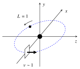
(a)	(b)

Figure 8: (a) Comparison of the leading–order chiral component of the nucleon’s isovector spin–independent current density $\rho_{1}^{V}(b)$ (solid line) and spin–dependent current density $\widetilde{\rho}_{2}^{V}(b)$ (dashed line). The plot shows the densities with the exponential factor $\exp(-2M_{\pi}b)$ extracted [the functions plotted correspond to the pre-exponential factor in Eq. (36)]. The distance $b$ is given in units of $M_{\pi}^{-1}$, the densities in units of $M_{\pi}^{2}$. (b) Mechanical picture explaining the relation of the peripheral densities (details see text). The nucleon state is polarized along the $y$–axis with $S^{y}=+1/2$. The peripheral densities are generated by components of the light–cone wave function involving a peripheral pion with $L=1$. At distances $b=O(M_{\pi}^{-1})$ the velocity of the pion is $v=O(1)$, and the current and charge density are of the same order.

The numerical results for the densities $\rho_{1}(b)$ and $\widetilde{\rho}_{2}(b)$, obtained from the leading–order chiral EFT result for the two–pion spectral functions, are compared in Fig. 8a. One sees that at all distances the chiral spin–dependent current density $\widetilde{\rho}_{2}^{V}(b)$ is smaller in absolute value than the spin–independent density $\rho_{1}^{V}(b)$,

$$|\widetilde{\rho}_{2}^{V}(b)|\;\;\leq\;\;\rho_{1}^{V}(b).$$ (132)

At smaller (but parametrically still “chiral”) distances $b\lesssim 2\,M_{\pi}^{-1}$ they become practically equal in absolute value. The inequality Eq. (132) implies that the chiral result for the total expectation value of the plus component of the isovector current, given by the sum of Eqs. (129) and (130) [cf. Eq. (32)], is positive

$$\langle J^{+}(\bm{b})\rangle = \rho_{1}^{V}(b)\;\;+\;\;(2S^{y})\,\cos\phi\,\widetilde{\rho}_{2}^{V}(b)\;\;\geq\;\;0.$$ (133)

We stress that Eqs. (132) and (133) are numerical statements based on inspection of the leading–order chiral results, and that we cannot claim that they hold under more general circumstances.

The two observations, Eqs. (131) and (133), can be explained in a simple quantum–mechanical picture of peripheral nucleon structure. Consider a nucleon with transverse spin $S^{y}=+1/2$ in the rest frame. The chiral component of the transverse densities at distances $b=O(M_{\pi}^{-1})$ arises from virtual processes in which the nucleon fluctuates into a $\pi N$ system through the effective chiral interactions. Because pion emission flips the nucleon spin, the relevant configurations in the wave function have the pion moving with orbital angular momentum $L=1$ (see Fig. 8b). The momentum of the peripheral pion is $k_{\pi}=O(M_{\pi})$, whence its velocity is $v=k_{\pi}/M_{\pi}=O(1)$; i.e., the motion of the pion is essentially relativistic. Since the $\pi N$ interaction is pointlike on the scale $M_{\pi}^{-1}$, we can regard the peripheral $\pi N$ system as non–interacting, and use this simple model to infer the expectation value of the current operator, including its light–cone component $J^{+}$. The spin–independent part of $J^{+}$ is given by the charge density $J^{0}$ in the rest frame, the spin–dependent part by the current density $J^{z}$. By simple geometry (see Fig. 8b) the ratio of current to charge density in the system is given by the pion velocity, and one obtains

$$\frac{|\langle J^{+}(\bm{b})\rangle_{\text{\scriptsize spin-dep.}}|}{\langle J^{+}(\bm{b})\rangle_{\text{\scriptsize spin-indep.}}}\;\;=\;\;\frac{|J^{z}|}{J^{0}}\;\;=\;\;v\;\;=\;\;O(1)\hskip 20.00003pt[b=O(M_{\pi}^{-1})],$$ (134)

which naturally explains Eq. (131). The positivity condition Eq. (133) can be accounted for in a similar manner. To the extent that the peripheral $\pi N$ system can be regarded as non–interacting, the current at $b=O(M_{\pi}^{-1})$ should be proportional to the current produced by a free charged pion with four–momentum $k$, which is

$$\langle\pi(\bm{k})|J^{+}|\pi(\bm{k})\rangle\;\ =\;\;2k^{+}\;\ >\;0,$$ (135)

where the last relation is obtained because $k^{0}=\sqrt{(k^{z})^{2}+\bm{k}_{T}^{2}+M_{\pi}^{2}}\geq|k^{z}|$ for a free particle. We emphasize that the mechanical picture presented here is just a heuristic tool, and that several aspects (role of relativity, non–interaction in the periphery) need to be clarified. A rigorous particle–based interpretation of the peripheral densities can be developed in the context of a time–ordered description of chiral processes and will be described elsewhere inprep .

In the molecular region, $b=O(M_{N}^{2}/M_{\pi}^{3})$, the asymptotic behavior of the densities $\rho_{1}$ and $\rho_{2}$ is described by Eqs. (114) and (116). One can easily see that this implies that the current matrix elements behave as

$$\frac{\widetilde{\rho}_{2}^{V}(b)}{\rho_{1}^{V}(b)} = O\left(\frac{M_{\pi}}{M_{N}}\right)\hskip 20.00003pt[b=O(M_{N}^{2}/M_{\pi}^{3})];$$ (136)

see also Eqs. (118) and (120). In this parametric region the spin–dependent part of the current matrix element is suppressed relative to the spin–independent one. The numerical results of Fig. 8a show that the ratio of the densities indeed decreases at distances $b\gg M_{\pi}^{-1}$. This behavior again can be understood in the mechanical picture of Fig. 8b. The analysis of Sec. II.4 shows that in this region of distances the pion velocity becomes parametrically small, $v=O(M_{\pi}/M_{N})$, cf. Eq. (66); using this result in the model estimate Eq. (134) one obtains exactly the parametric suppression Eq. (136) .

III.5 Contact terms and pseudoscalar $\pi N$ coupling

The presence of a $\pi\pi NN$ contact term in the leading–order chiral EFT results for the isovector Dirac spectral function and transverse charge density is a matter that merits separate discussion. In fact, the compact expressions obtained in Sec. III.2 shed new light on the physical interpretation of this structure.

The pion–nucleon contact couplings in the chiral Lagrangian Eq. (67) encode the effect of internal structure of the nucleon which is not resolved by pions with moment $k=O(M_{\pi})$. In the isovector Dirac spectral function, the $\pi\pi NN$ contact term in the Lagrangian, exhibited explicitly in Eq. (71), induces a chiral process in which the two pions couple to the nucleon locally on the scale $O(M_{\pi}^{-1})$, described by diagram Fig. 3b. A local contribution of the same structure arises also from diagram Fig. 3a, as a term in which the numerator cancels the pole of the intermediate nucleon propagator. This results in a net contact term with coefficient [cf. Eq. (79)]

$$\frac{1-g_{A}^{2}}{F_{\pi}^{2}}$$ (137)

in the Dirac spectral function and transverse charge density. The appearance of the combination $1-g_{A}^{2}$ here is very natural. For a pointlike (i.e., structureless) Dirac fermion the axial coupling is unity, $g_{A}=1$, as can be seen trivially by computing the matrix element of the axial vector current between free–particle states. The combination Eq. (137) thus vanishes for a pointlike particle and reflects the “compositeness” of the nucleon. It would be interesting to explore the connection between $g_{A}>1$ and the $\pi\pi NN$ contact coupling at a more microscopic level. For example, using a composite model of nucleon structure, with pions coupling to quarks, one might be able to demonstrate explicitly that both effects arise from the same underlying dynamics .

The presence of contact terms in the chiral Lagrangian is closely related to the form of the basic $\pi NN$ coupling adopted in formulating the effective dynamics. The $\pi\pi NN$ contact term of Eq. (71) is specific to the axial vector form of the $\pi NN$ coupling. It is well–known that for on–shell nucleons this form is equivalent to the pseudoscalar form of the $\pi NN$ coupling, cf. Eq. (72), if one identifies $g_{\pi NN}=M_{N}g_{A}/F_{\pi}$. [More generally, the axial–vector chiral Lagrangian Eq. (71), including the $\pi\pi NN$ contact term, can be obtained from a pseudoscalar Langrangian by performing a chiral rotation of the nucleon fields with the matrices $U^{\pm 1/2}$, Eq. (70). The contact arises from the chiral rotation of the pseudoscalar kinetic term and therefore carries the universal coefficient $\sim 1/F_{\pi}^{2}$.] It is interesting to note that we get the same result for the intermediate nucleon (or “non–contact”) part of the isovector Dirac spectral function, Eq. (92), with the pseudoscalar and axial vector forms of the $\pi NN$ couplings Strikman:2010pu . This part arises from the triangle graph Fig. 3a with the intermediate nucleon propagator, after separating out the off–shell terms in the numerator [keeping only the third term in Eq. (78)], and one can verify by explicit calculation that the result is the same as what one obtains with a pseudoscalar coupling given by Eq. (72). It shows that the difference between the pseudoscalar and axial vector couplings is effectively contained in the “net” $\pi\pi NN$ contact term in the final result, Eq. (93), which is again consistent with this term being proportional to $1-g_{A}^{2}$ and reflecting the compositeness of the nucleon.

In the light–front formulation of chiral processes the contact terms summarize the contributions from quasi–zero modes, in which the pion field carries a vanishing fraction of the nucleon’s plus momentum Strikman:2010pu . This can be shown explicitly by following the space–time–evolution of the chiral processes in time–ordered perturbation theory inprep . It is also known that in time–ordered perturbation theory the different forms of the $\pi N$ coupling give apparently different results, as this formulation of relativistic dynamics does not conserve four–momentum in intermediate states Ji:2009jc ; Burkardt:2012hk . Our findings suggest that there is a natural connection between the two observations.

IV Delta isobar and large–$N_{c}$ limit

IV.1 Peripheral densities from $\Delta$ excitation

We now want to study the role of $\Delta$ isobar excitation in the nucleon’s peripheral transverse charge and magnetization densities. While going beyond the domain of strictly chiral dynamics, inclusion of the $\Delta$ is important for practical as well as theoretical reasons. First, the $\pi N\Delta$ coupling is large, and $N\rightarrow\pi\Delta$ transitions contribute significantly to the isovector spectral functions at $t-4M_{\pi}^{2}\sim\textrm{few}\,M_{\pi}^{2}$ and the transverse densities at $b\sim\textrm{few}\,M_{\pi}^{-1}$. Second, with the $\Delta$ we can see explicitly how the analytic structure of the form factor near the two–pion threshold changes in the case of a “heavy” intermediate state, and how the mass splitting affects the subthreshold singularity that plays such an important role in the amplitude with the nucleon intermediate state. Third, and most important, inclusion of the $\Delta$ is required to ensure the proper scaling behavior of the peripheral densities in the large–$N_{c}$ limit of QCD.

The $N\Delta$ mass splitting $M_{\Delta}-M_{N}=0.29\,\textrm{GeV}$ represents a “non–chiral” mass scale that is numerically comparable to the pion mass $M_{\pi}=0.14\,\textrm{GeV}$. Several schemes for extending chiral EFT to include $\Delta$ degrees of freedom have been proposed, putting the $N\Delta$ mass splitting in some parametric relation to the pion mass. Our objectives here are very specific and can be addressed without a fully developed EFT of the $\Delta$. We want to estimate the contribution of intermediate $\Delta$ states in the two–pion cut of the isovector spectral function and the peripheral densities in a way that is consistent with the leading–order relativistic chiral EFT treatment of the nucleon of Sec. III, and verify that the total result obeys the proper $N_{c}$–scaling. To this end we introduce the $\Delta$ as a relativistic point particle, with an empirical $\pi N\Delta$ coupling, and treat the $N\Delta$ mass splitting as a free parameter, with no defined relation to $M_{\pi}$; later, we let the masses and couplings scale according to their large–$N_{c}$ behavior.

The spin–3/2 field of the $\Delta$ can be constructed by applying constraints to a four–vector bispinor field (Rarita–Schwinger formalism) LLIV . Its Green function with four–momentum $l$ is

$$\frac{R_{\mu\nu}(l)}{l^{2}-M_{\Delta}^{2}+i0},$$ (138)

where the projector is explicitly given by

$$R_{\mu\nu}(l) \equiv (\hat{l}+M_{\Delta})\left[-g_{\mu\nu}+\frac{1}{3}\gamma_{\mu}\gamma_{\nu}+\frac{2}{3M_{\Delta}^{2}}l_{\mu}l_{\nu}-\frac{1}{3M_{\Delta}}(l_{\mu}\gamma_{\nu}-\gamma_{\mu}l_{\nu})\right]$$ (139)

$$= (\hat{l}+M_{\Delta})\left(-g_{\mu\nu}+\frac{l_{\mu}l_{\nu}}{M_{\Delta}^{2}}\right)\;-\;\frac{1}{3}\left(\gamma_{\mu}+\frac{l_{\mu}}{M_{\Delta}}\right)(\hat{l}-M_{\Delta})\left(\gamma_{\nu}+\frac{l_{\nu}}{M_{\Delta}}\right)$$ (140)

and obeys the constraints

$$\left.\begin{array}[]{r}l_{\mu}R_{\mu\nu}\\[4.30554pt] R_{\mu\nu}l_{\nu}\\[4.30554pt] (\hat{l}-M_{\Delta})R_{\mu\nu}\\[4.30554pt] R_{\mu\nu}(\hat{l}-M_{\Delta})\end{array}\right\}\;\;\propto\;\;(l^{2}-M_{\Delta}^{2}),$$ (141)

implying that in the corresponding contractions the pole of the Green function is canceled. The $\pi N\Delta$ interaction is described by the Lagrangian

$$\mathcal{L}_{\pi N\Delta} = \frac{ig_{\pi N\Delta}}{\sqrt{2}M_{N}}\left[\bar{\psi}_{p}\;\partial_{\mu}\pi^{-}\;\Psi_{\Delta++}^{\mu}+\sqrt{\frac{2}{3}}\;\bar{\psi}_{p}\;\partial_{\mu}\pi^{0}\;\Psi_{\Delta+}^{\mu}+\frac{1}{\sqrt{3}}\;\bar{\psi}_{p}\;\partial_{\mu}\pi^{+}\;\Psi_{\Delta 0}^{\mu}\right.$$ (142)

$$+ \left.\bar{\psi}_{n}\;\partial_{\mu}\pi^{+}\;\Psi_{\Delta-}^{\mu}+\sqrt{\frac{2}{3}}\;\bar{\psi}_{n}\;\partial_{\mu}\pi^{0}\;\Psi_{\Delta 0}^{\mu}+\frac{1}{\sqrt{3}}\;\bar{\psi}_{n}\;\partial_{\mu}\pi^{-}\;\Psi_{\Delta+}^{\mu}\right]\;\;+\;\;\mbox{h.c.},$$

where $\psi_{p,n}$ are the proton and neutron fields and $\Psi_{\Delta++}^{\mu}$ etc. the $\Delta$ fields. The relative coefficients of the terms in Eq. (142) are dictated by isospin invariance. Our definition of the coupling constant $g_{\pi N\Delta}$ corresponds to that of Ref. Adkins:1983ya (see Refs. Strikman:2003gz ; Strikman:2009bd for comparison with other conventions), and the empirical value of the coupling is $g_{\pi N\Delta}=20.22$. We note that the introduction of the $\Delta$ into the effective Lagrangian could in principle result in, or require, the addition of a $\pi\pi NN$ contact term of the same type as that already present in the $\pi N$ Lagrangian; the physical meaning and implications of such a term are discussed below.

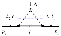
Figure 9: Contribution of $\Delta$ isobar excitation to the two–pion cut of the isovector nucleon form factor. The labeling of the 4–momenta is the same as for the intermediate $N$ diagram of Fig. 3a.

With the coupling Eq. (142) and the Green function Eq. (138) it is straightforward to calculate the contribution of $N\rightarrow\Delta$ transitions to the two–pion cut of the isovector spectral functions. The calculation closely follows that for the intermediate nucleon state in Sec. III.1, and we outline only the main steps. The $\Delta$ contribution to the isovector current matrix element, as given by diagram Fig. 9, is

$$\langle N_{2}|J^{\mu}(0)|N_{1}\rangle_{\pi\pi\;{\rm cut}} = -\frac{2ig_{\pi N\Delta}^{2}}{3M_{N}^{2}}\int\frac{d^{4}k}{(2\pi)^{4}}\frac{[\bar{u}_{2}\,k_{2\alpha}R_{\alpha\beta}(l)k_{1\beta}\,u_{1}]\,k^{\mu}}{(k_{2}^{2}-M_{\pi}^{2}+i0)(k_{1}^{2}-M_{\pi}^{2}+i0)(l^{2}-M_{\Delta}^{2}+i0)},$$ (143)

where again $u_{1,2}$ are the external nucleon bispinors and the labeling of the 4–momenta is the same as in the case of the intermediate nucleon diagram Fig. 3a, Eq. (74). The bilinear form in the numerator contains terms which vanish at $s\equiv l^{2}=M_{\Delta}^{2}$ and result in integrals of the same form as that obtained from the $\pi\pi NN$ contact term, Eq. (75). Making extensive use of the constraints Eq. (141) [the result of the particular contractions has to be determined from Eqs. (139) or (140)], the kinematic relations between the different momentum 4-vectors, and the Dirac equation for the external nucleon spinors, we write the bilinear form as

$$\bar{u}_{2}\,k_{2\alpha}R_{\alpha\beta}(l)k_{1\beta}\,u_{1} = \bar{u}_{2}(F+G\,\hat{k})u_{1}\;+\;(s-M_{\Delta}^{2})\bar{u}_{2}R_{\rm off}u_{1}.$$ (144)

The first term on the right–hand side remains non–zero on the baryon mass–shell. Here $F$ and $G$ denote scalar functions of the invariants $t$ and $k_{1,2}^{2}=(k\mp\Delta/2)^{2}$,

$$\left.\begin{array}[]{r}F(t,k_{1}^{2},k_{2}^{2})\\[8.61108pt] G(t,k_{1}^{2},k_{2}^{2})\end{array}\right\} \equiv \left[\frac{t}{2}-M_{N}^{2}+\frac{(M_{\Delta}^{2}+M_{N}^{2}-k_{2}^{2})(M_{\Delta}^{2}+M_{N}^{2}-k_{1}^{2})}{4M_{\Delta}^{2}}\right]\;\times\;\left\{\begin{array}[]{c}(M_{\Delta}+M_{N})\\[8.61108pt] (-1)\end{array}\right\}$$ (149)

$$+ \frac{1}{3}\left(M_{N}+\frac{M_{\Delta}^{2}+M_{N}^{2}-k_{2}^{2}}{2M_{\Delta}}\right)\left(M_{N}+\frac{M_{\Delta}^{2}+M_{N}^{2}-k_{1}^{2}}{2M_{\Delta}}\right)\;\times\;\left\{\begin{array}[]{c}(M_{\Delta}-M_{N})\\[8.61108pt] 1\end{array}\right\}.$$ (152)

Note that the functions are symmetric with respect to both $k\rightarrow-k$ and $\Delta\rightarrow-\Delta$. The second term in Eq. (144) is an off–shell piece, with

$$R_{\rm off} \equiv \frac{1}{3M_{\Delta}^{2}}\left[M_{\Delta}^{2}-M_{N}^{2}+M_{N}M_{\Delta}+M_{\pi}^{2}+\frac{1}{4}(s-M_{\Delta}^{2})\right](M_{N}+M_{\Delta}-\hat{k})$$ (153)

$$+ \frac{(s-M_{\Delta}^{2})}{12\,M_{\Delta}^{2}}(M_{N}-M_{\Delta}-\hat{k}),$$

where $s=l^{2}=(P-k)^{2}$. After inserting the decomposition Eq. (144) into Eq. (143), the tensor integrals are reduced to scalar integrals with the help of standard projection formulas, making use of the symmetries of the integrand. The resulting bilinear forms $\bar{u}_{2}\ldots u_{1}$ are then converted to those of the right–hand side of Eq. (1) using the Dirac equation for the nucleon spinors. In this way we obtain the $\Delta$ contribution to the isovector Dirac and Pauli form factors in terms of invariant integrals as

$$F_{1}^{V}(t)_{\pi\pi\;{\rm cut}} = \frac{2g_{\pi N\Delta}^{2}}{3M_{N}^{2}}\,\left[I_{\Delta 1}(t)\;+\;I_{\Delta 1\,{\rm cont}}(t)\right],$$ (154)

$$F_{2}^{V}(t)_{\pi\pi\;{\rm cut}} = \frac{2g_{\pi N\Delta}^{2}}{3M_{N}^{2}}\,\left[I_{\Delta 2}(t)\;+\;I_{\Delta 2\,{\rm cont}}(t)\right],$$ (155)

$$I_{\Delta 1,\,\Delta 2} \equiv -i\int\frac{d^{4}k}{(2\pi)^{4}}\frac{N_{\Delta 1,\,\Delta 2}}{(k_{2}^{2}-M_{\pi}^{2}+i0)(k_{1}^{2}-M_{\pi}^{2}+i0)(l^{2}-M_{\Delta}^{2}+i0)},$$ (156)

$$N_{\Delta 1} = \frac{kP}{P^{2}}M_{N}\,F\;+\;\frac{1}{P^{2}}\left\{-\frac{t}{8}\left[k^{2}-\frac{(k\Delta)^{2}}{\Delta^{2}}\right]\;+\;\left(M_{N}^{2}+\frac{t}{8}\right)\frac{(kP)^{2}}{P^{2}}\right\}\,G,$$ (157)

$$N_{\Delta 2} = -\frac{kP}{P^{2}}M_{N}\,F\;-\;\frac{M_{N}^{2}}{P^{2}}\left[-k^{2}+3\frac{(kP)^{2}}{P^{2}}+\frac{(k\Delta)^{2}}{\Delta^{2}}\right]\frac{G}{2},$$ (158)

$$I_{\Delta 1\,{\rm cont},\;\Delta 2\,{\rm cont}} = -i\int\frac{d^{4}k}{(2\pi)^{4}}\frac{N_{\Delta 1\,{\rm cont},\;\Delta 2\,{\rm cont}}}{(k_{2}^{2}-M_{\pi}^{2}+i0)(k_{1}^{2}-M_{\pi}^{2}+i0)},$$ (159)

$$N_{\Delta 1\,{\rm cont}} = \frac{1}{3M_{\Delta}^{2}}\left[k^{2}-\frac{(k\Delta)^{2}}{\Delta^{2}}\right]\left[-\frac{k^{2}}{2}-\frac{1}{6}(M_{N}+M_{\Delta})^{2}-\frac{t}{24}\right],$$ (160)

$$N_{\Delta 2\,{\rm cont}} = \frac{M_{N}^{2}}{9M_{\Delta}^{2}}\left[k^{2}-\frac{(k\Delta)^{2}}{\Delta^{2}}\right].$$ (161)

The imaginary part on the two–pion cut can now be computed using the $t$–channel cutting rule of Appendix A in the same way as in the intermediate nucleon case. The virtuality of the intermediate $\Delta$ is

$$l^{2}-M_{\Delta}^{2} = -A_{\Delta}+iB\cos\theta,$$ (162)

$$A_{\Delta} \equiv t/2-M_{\pi}^{2}+M_{\Delta}^{2}-M_{N}^{2},$$ (163)

$$B \equiv 2k_{\rm cm}\sqrt{P^{2}}.$$ (164)

We obtain the spectral functions as

$$\frac{1}{\pi}\,\textrm{Im}\,F_{1}^{V}(t) = \frac{g_{\pi N\Delta}^{2}}{24\pi^{2}M_{N}^{2}\sqrt{P^{2}}\sqrt{t}}\left\{-\frac{A_{\Delta}M_{N}F}{2P^{2}}(x_{\Delta}-\arctan x_{\Delta})\right.$$ (165)

$$+ \left.\frac{A_{\Delta}^{2}G}{4(P^{2})^{2}}\left[-\frac{t}{8}x_{\Delta}^{2}\arctan x_{\Delta}+\left(M_{N}^{2}+\frac{t}{8}\right)(x_{\Delta}-\arctan x_{\Delta})\right]\right\}$$

$$+ \frac{g_{\pi N\Delta}^{2}k_{\rm cm}^{3}}{36\pi^{2}M_{N}^{2}M_{\Delta}^{2}\sqrt{t}}\left[-\frac{k_{\rm cm}^{2}}{2}+\frac{1}{6}(M_{N}+M_{\Delta})^{2}+\frac{t}{24}\right],$$ (166)

$$\frac{1}{\pi}\,\textrm{Im}\,F_{2}^{V}(t) = \frac{g_{\pi N\Delta}^{2}}{24\pi^{2}M_{N}^{2}\sqrt{P^{2}}\sqrt{t}}\left\{\frac{M_{N}A_{\Delta}F}{2P^{2}}(x_{\Delta}-\arctan x_{\Delta})\right.$$ (167)

$$+ \left.\frac{M_{N}^{2}A_{\Delta}^{2}G}{8(P^{2})^{2}}\left[(x_{\Delta}^{2}+3)\arctan x_{\Delta}-3x_{\Delta}\right]\right\}$$

$$- \frac{g_{\pi N\Delta}^{2}k_{\rm cm}^{3}}{108\pi^{2}M_{\Delta}^{2}\sqrt{t}},$$ (168)

$$x_{\Delta} \equiv \frac{B}{A_{\Delta}}\;\;=\;\;\frac{2\sqrt{t/4-M_{\pi}^{2}}\sqrt{M_{N}^{2}-t/4}}{t/2-M_{\pi}^{2}+M_{\Delta}^{2}-M_{N}^{2}},$$ (169)

where $F$ and $G$ now denote the functions of Eq. (152) on the pion mass shell,

$$F \equiv F(t,\;k_{1}^{2}=M_{\pi}^{2},\;k_{2}^{2}=M_{\pi}^{2})$$ (170)

$$= \left[\frac{t}{2}-M_{N}^{2}+\frac{(M_{\Delta}^{2}+M_{N}^{2}-M_{\pi}^{2})^{2}}{4M_{\Delta}^{2}}\right](M_{N}+M_{\Delta})-\frac{1}{3}\left(M_{N}+\frac{M_{\Delta}^{2}+M_{N}^{2}-M_{\pi}^{2}}{2M_{\Delta}}\right)^{2}(M_{N}-M_{\Delta}),$$

$$G \equiv G(t,\;k_{1}^{2}=M_{\pi}^{2},\;k_{2}^{2}=M_{\pi}^{2})$$ (171)

$$= -\left[\frac{t}{2}-M_{N}^{2}+\frac{(M_{\Delta}^{2}+M_{N}^{2}-M_{\pi}^{2})^{2}}{4M_{\Delta}^{2}}\right]+\frac{1}{3}\left(M_{N}+\frac{M_{\Delta}^{2}+M_{N}^{2}-M_{\pi}^{2}}{2M_{\Delta}}\right)^{2}.$$

For further analysis it will be convenient to quote simplified expressions according to the uniform approximation, Eqs. (126)–(128), in which we neglect terms $t/M_{N}^{2}$ without altering the analytic structure near threshold. In the contact term Eq. (166) we can also neglect terms of order $t/M_{N,\Delta}^{2}$ and $M_{\pi}^{2}/M_{N,\Delta}^{2}$. With these approximations we obtain

$$\frac{1}{\pi}\,\textrm{Im}\,F_{1}^{V}(t) = \frac{g_{\pi N\Delta}^{2}\,A_{\Delta}(-2M_{N}F+A_{\Delta}G)}{96\pi^{2}M_{N}^{5}\sqrt{t}}(x_{\Delta 1}-\arctan x_{\Delta 1})$$ (172)

$$+ \frac{g_{\pi N\Delta}^{2}(M_{N}+M_{\Delta})^{2}k_{\rm cm}^{3}}{216\pi^{2}M_{N}^{2}M_{\Delta}^{2}\sqrt{t}},$$ (173)

$$\frac{1}{\pi}\,\textrm{Im}\,F_{2}^{V}(t) = \frac{g_{\pi N\Delta}^{2}\,A_{\Delta}}{192\pi^{2}M_{N}^{5}\sqrt{t}}\left[(4M_{N}F-3A_{\Delta}G)\,(x_{\Delta 1}-\arctan x_{\Delta 1})\;+\;A_{\Delta}G\,x_{\Delta 1}^{2}\arctan x_{\Delta 1}\right]$$ (174)

$$- \frac{g_{\pi N\Delta}^{2}k_{\rm cm}^{3}}{108\pi^{2}M_{\Delta}^{2}\sqrt{t}},$$ (175)

$$x_{\Delta 1} \equiv x_{\Delta 1}(t)\;\;\equiv\;\;\frac{2M_{N}k_{\rm cm}}{A_{\Delta}}\;\;=\;\;\frac{2M_{N}\sqrt{t/4-M_{\pi}^{2}}}{t/2-M_{\pi}^{2}+M_{\Delta}^{2}-M_{N}^{2}}.$$ (176)

Equations (172)–(176) provide a compact and completely adequate representation of the two–pion spectral functions resulting from $\Delta$ intermediate states.

(a)	(b)

Figure 10: Comparison of chiral and $\Delta$ contributions to the spectral functions of the isovector Dirac form factor $\textrm{Im}\,F_{1}^{V}(t)/\pi$ [panel (a)] and Pauli form factor $\textrm{Im}\,F_{2}^{V}(t)/\pi$ [panel (b)]. Solid lines: Chiral component, intermediate $N$, Eq. (92). Dotted line: Chiral component, contact term Eq. (93) [in the Pauli form factor in plot (b) this term is absent]. Dashed lines: Contribution from intermediate $\Delta$, Eq. (165). Dashed–dotted line: $\Delta$ contact term.

The numerical results for the two–pion isovector spectral functions resulting from $\Delta$ intermediate states, Eqs. (165)–(171), are shown in Fig. 10, together with those from $N$ intermediate states, Eqs. (92)–(III.1). Several features are worth noting. First, in the Dirac spectral function in Fig. 10a the $N$ and $\Delta$ contributions have opposite sign, both in the contact and non–contact terms, such that they partly cancel each other. In the Pauli spectral function in Fig. 10b, in contrast, the $N$ and $\Delta$ contributions have the same sign. Both findings can naturally be explained in the large–$N_{c}$ limit of QCD, where model–independent relations between the $N$ and $\Delta$ spectral functions can be derived (see Sec. IV.3). Second, the $\Delta$ contributions do not show the strong rise near threshold observed in the intermediate $N$ contributions to the Dirac and Pauli spectral functions. This is because in the intermediate $\Delta$ case the subthreshold singularity is removed from threshold by a much larger distance, see Eq. (58). It implies that the transverse densities at large distances are dominated by the contribution from intermediate $N$ states, as expected.

A comment is in order regarding the interpretation of the contact terms in the $\Delta$ contribution to the Dirac spectral function. Equation (166) represents the contact term as it comes out of the diagram of Fig. 9. It is seen from Fig. 10a that numerically this term is considerably larger than the net contact term in the chiral EFT result with nucleons only, Eq. (93). The latter is the sum of the explicit contact term in the chiral Lagrangian entering in diagram Fig. 3b, and the “non–propagating” piece of the diagram of Fig. 3a, with substantial cancellations between the two, cf. Eq. (79). From a physical point of view, inclusion of the $\Delta$ as an explicit degree of freedom in the chiral Lagrangian amounts to a change of the short–distance structure of the nucleon, which could manifest itself in the appearance of a “new” $\pi\pi NN$ contact term, or, effectively, a renormalization of the old contact term in the chiral Lagrangian. Unlike the case of the Lagrangian with $N$ only, the strength of this new contact term is not fixed by chiral symmetry, and we presently have no way to constrain it theoretically. It is likely that this new contact term would partly cancel the contact term coming out of the $\Delta$ diagram of Fig. 9. Because we cannot determine the coefficient of the total contact term from general principles, and because the $\Delta$ effects are altogether rather unimportant at large distances, we shall treat the $\Delta$ contact term in the Dirac spectral function as a theoretical uncertainty (see below).

A contact term is also found in the $\Delta$ contribution to the Pauli spectral function, Eq. (168). However, its contribution is extremely small, see Fig. 10b, and we shall nexlect the theoretical uncertainty associated with it. Note that in this channel there is no contact term in the chiral EFT result with nucleons only, Eq. (94).

(a)	(b)

Figure 11: Effect of $\Delta$ excitation on the peripheral isovector transverse charge and magnetization densities of the nucleon. The plots shows the densities $\rho_{1,2}^{V}(b)$ with the exponential factor $\exp(-2M_{\pi}b)$ extracted (cf. Fig. 6b). The distance $b$ is given in units of $M_{\pi}^{-1}$, the densities in units of $M_{\pi}^{2}$. (a) Transverse charge density $\rho_{1}(b)$. Solid line: Chiral component from intermediate $N$ states and the $N$ contact term, Eqs. (92) and Eqs. (93). Dotted lines: Sum of chiral component (solid line) and $\Delta$ contribution, Eqs. (166)–(165). The two curves show the results obtained with the $\Delta$ contact term, Eq. (166), multiplied by 0 and 2, respectively; their difference is an estimate of the theoretical uncertainty (details see text). (b) Transverse magnetization density $\rho_{2}(b)$. Solid line: Chiral component from intermediate $N$ states, Eq. (94). Dotted line: Sum of chiral and $\Delta$ contributions, Eqs. (168)–(167). The uncertainty resulting from the $\Delta$ contact term is negligible on the scale of the plot and not shown on the figure.

Using the results for the spectral functions we can now calculate the peripheral transverse densities resulting from $\Delta$ intermediate states. Figure 11a summarizes the numerical effect of the $\Delta$ on the transverse charge density. The solid line shows the chiral component with intermediate $N$ states only (see Fig. 6a). The dotted lines show the density after adding the $\Delta$ contribution. The lower curve is obtained when including the contact term Eq. (166) with full strength, the lower curve when setting it to zero, as would correspond to complete cancellation by an explicit new $\pi\pi NN$ contact term in the Lagrangian (cf. the discussion of the theoretical uncertainty above). One sees that at $b\lesssim 1\,M_{\pi}^{-1}$ there are very substantial cancellations between the $N$ and $\Delta$ contributions, causing the total two–pion isovector density from intermediate $N$ and $\Delta$ to become negative at small $b$. [Note that the physical density at such small values of $b$ is dominated by vector meson singularity of the spectral function (see Sec. V), and that Fig. 11a is only intended to illustrate the relative magnitude of the calculated $N$ and $\Delta$ contributions.] At distances $b\gtrsim 2\,M_{\pi}^{-1}$ the $\Delta$ contribution becomes a small correction of $\sim 20\%$, as expected from a “heavy” degree of freedom. The theoretical uncertainty associated with the inclusion of the $\Delta$ therefore does not affect our numerical estimates of the chiral component of the transverse charge density.

Figure 11b shows the effect of the $\Delta$ on the transverse magnetization density. At distances $b\gtrsim 2\,M_{\pi}^{-1}$ the $\Delta$ increases the intermediate $N$ result by $\sim 20\%$. One sees that the effect of the $\Delta$ has opposite sign in the charge and magnetization densities, as already noted in relation to the spectral functions. This pattern is naturally explained by the relations between the intermediate $N$ and $\Delta$ contributions emerging in the large–$N_{c}$ limit of QCD.

IV.2 Transverse densities in large–$N_{c}$ QCD

The limit of a large number of colors in QCD, $N_{c}\rightarrow\infty$, is a powerful theoretical tool for studying properties of mesons and baryons and relating them to the microscopic theory of strong interactions. While even in the large–$N_{c}$ limit QCD remains a complex dynamical system that cannot be solved exactly, the scaling behavior of meson and baryon properties with $N_{c}$ can be established on general grounds and provides constraints for EFTs or phenomenological models. In this subsection we want to establish the $N_{c}$–scaling behavior of the transverse charge and magnetization densities on general grounds. In the following subsection we then show that the two–pion components of the peripheral charge and magnetization densities obey these general scaling laws and discuss the essential role of $\Delta$ isobar excitation in bringing about this result.

The $N_{c}$–scaling of meson and baryon masses in QCD, their interactions, and various current matrix elements, can be established using the classic techniques described in Ref. Witten:1979kh . It is found that the low–lying meson and baryon masses [i.e., with spin and isospin of $O(N_{c}^{0})$] scale as

$$M_{\textrm{\scriptsize meson}}\;\;=\;\;O(N_{c}^{0}),\hskip 20.00003ptM_{\textrm{\scriptsize baryon}}\;\;=\;\;O(N_{c}),$$ (177)

while their basic hadronic sizes scale as

$$R_{\textrm{\scriptsize meson}},\,R_{\textrm{\scriptsize baryon}}\;\;=\;\;O(N_{c}^{0}).$$ (178)

Baryons in large–$N_{c}$ QCD thus are heavy systems of fixed spatial size. Their overall momentum and spin–isospin degrees of freedom can be described as the classical motion of a heavy body characterized by a mass and moment of inertia of order $O(N_{c})$. In particular, the $N$ and $\Delta$ are obtained as rotational states with $S=T=1/2$ and $S=T=3/2$, and their mass splitting is $M_{\Delta}-M_{N}=O(N_{c}^{-1})$. This description can be extended to transition matrix elements of current operators, which generally involve new parameters characterizing the internal structure of the classical rotor, and has been formalized using group–theoretical methods Dashen:1993jt ; Dashen:1994qi .

Turning to the transverse charge and magnetization densities, we are interested in their general $N_{c}$–scaling behavior at non–exceptional distances of the order

$$b\;\;=\;\;O(N_{c}^{0}),$$ (179)

i.e., distances of the same order as the basic hadronic size of the large–$N_{c}$ nucleon, Eq. (178). [Below we shall see that the chiral component is contained in this parametric region, as it involves distances of the order $b=O(M_{\pi}^{-1})$ and the pion mass scales as $M_{\pi}=O(N_{c}^{0})$.] For such distances the $N_{c}$–scaling behavior of the density can be inferred from that of the corresponding total charge, given by the integral of the density over $b$. The isovector densities are normalized, respectively, to the total isovector charge and anomalous magnetic moment of the nucleon, which scale as

$$\int d^{2}b\;\rho_{1}^{V}(b) = \;\frac{1}{2}\;\;=\;\;O(N_{c}^{0}),$$ (180)

$$\int d^{2}b\;\frac{\rho_{2}^{V}(b)}{M_{N}} = \frac{\kappa_{p}-\kappa_{n}}{2M_{N}}\;\;=\;\;O(N_{c}).$$ (181)

Here we assume that the large–$N_{c}$ limit is taken at fixed spin and isospin of the baryon states, $\{S,T\}=O(N_{c}^{0})$, which is the domain usually considered in large–$N_{c}$ phenomenology . The scaling behavior of the isospin difference Eq. (180) is immediately obvious. The scaling behavior of the isovector anomalous magnetic moment, Eq. (181), can be established in various ways, e.g., by explicitly constructing the spin–flavor wave functions of the nonrelativistic quark model at large $N_{c}$ Karl:1984cz ; Jackson:1985bn . It is important to realize that the $N_{c}$ scaling thus obtained applies to the dimensionful isovector magnetic moment of the nucleon, while the dimensionless quantity $\kappa_{p}-\kappa_{n}$ measures the isovector anomalous magnetic moment in units of the nuclear magneton $e/(2M_{N})$; one therefore needs to explicitly include the factors $1/M_{N}=O(N_{c}^{-1})$ in the $N_{c}$ scaling relation, as done in Eq. (181). Because the range of the $b$–integration remains stable in the large–$N_{c}$ limit, the scaling behavior of the densities follows that of the charges, and we conclude that

$$\rho_{1}^{V}(b)\;\;=\;\;O(N_{c}^{0}),\hskip 20.00003pt\frac{\rho_{2}^{V}(b)}{M_{N}}\;\;=\;\;O(N_{c})\hskip 20.00003pt[b=O(N_{c}^{0})].$$ (182)

Equation (182) represents the general scaling behavior of the isovector densities at non–exceptional distances in large–$N_{c}$ QCD. One sees that the physical isovector magnetization density (including the factor $1/M_{N}$) is parametrically larger than the isovector charge density. This is a consequence of the spin–flavor symmetry of the large–$N_{c}$ nucleon, which implies that the spin–dependent matrix elements of isovector quark operators are larger than the spin–independent ones by one order in $N_{c}$, and represents a general pattern that is found also in matrix elements of other operators. We note that the $N_{c}$–scaling relations Eq. (182) for the transverse densities could also be obtained from the more general scaling relations for the isovector nucleon GPDs $H^{u-d}(x,\xi,t)$ and $E^{u-d}(x,\xi,t)$ described in Ref. Goeke:2001tz , by integrating the latter over the quark momentum fraction $x=O(N_{c}^{-1})$, setting $\xi=0$, and performing the transverse Fourier transform as in Eq. (13) with $t=-\Delta_{T}^{2}=O(N_{c}^{0})$.

IV.3 Two–pion component in large–$N_{c}$ limit

We now want to examine the $N_{c}$–scaling of the two–pion component of the transverse densities calculated in Secs. III.1 and IV.1. This exercise explains the interplay between the $N$ and $\Delta$ contributions observed in Sec. IV.1 and provides a powerful check on the calculations. More generally, it shows that the two–pion component calculated using EFT methods obeys the large–$N_{c}$ scaling laws required by QCD.

Some general comments are in order regarding the compatibility of the large–$N_{c}$ limit of QCD with our identification of the chiral component based on the spatial picture of nucleon structure. First, in our approach we are interested in the transverse densities at distances $b\sim M_{\pi}^{-1}$, where $M_{\pi}^{-1}$ is assumed to be parametrically large compared to the nucleon’s non–chiral size but we do not actually take the limit $M_{\pi}\rightarrow 0$. Since the pion mass scales as $M_{\pi}=O(N_{c}^{0})$ this region of distances remains stable in the large–$N_{c}$ limit,

$$b\;\;\sim\;\;M_{\pi}^{-1}\;\;=O(N_{c}^{0}),$$ (183)

as does the nucleon’s non–chiral hadronic size, Eq. (178). As a result, the basic proportion of the non-chiral and chiral regions of nucleon structure does not change in the large–$N_{c}$ limit, and the latter is naturally compatible with our spatial picture. Second, in the large–$N_{c}$ limit both the $N$ and the $\Delta$ become heavy, so that this limit corresponds to the heavy–baryon expansion of the densities. All the findings of Sec. III.3, in particular the various consequences of the vanishing distance of the subthreshold singularity from the physical threshold, can be carried over to the discussion of the large–$N_{c}$ limit.

Using the explicit expressions for the leading–order chiral EFT result for the two–pion spectral functions Eqs. (92)–(III.1), we can determine the $N_{c}$–scaling of the corresponding components of the transverse densities. With the general scaling relations for the couplings

$$g_{A}\;=\;O(N_{c}),\hskip 20.00003ptF_{\pi}\;=\;O(N_{c}^{1/2}),$$ (184)

and the masses, Eq. (177), we find that for $t=O(M_{\pi}^{2})=O(N_{c}^{0})$ the spectral functions scale as

$$\textrm{Im}\,F_{1}^{V}(t)_{N} = O(N_{c}),$$ (185)

$$\frac{\textrm{Im}\,F_{2}^{V}(t)_{N}}{M_{N}} = O(N_{c})\hskip 20.00003pt[t=O(N_{c}^{0})].$$ (186)

The subscript $N$ here indicates that these are the results obtained from the chiral EFT with nucleons only (including the contributions from intermediate $N$ states and the contact term) and distinguishes them from the $\Delta$ contribution considered below. In the dispersion integral Eq. (34) this implies that

$$\rho_{1}^{V}(b)_{N} = O(N_{c}),$$ (187)

$$\frac{\rho_{2}^{V}(b)_{N}}{M_{N}} = O(N_{c})\hskip 20.00003pt[b=O(N_{c}^{0})].$$ (188)

These results can also be obtained directly from the heavy–baryon expansion of the densities in the chiral region $b=O(M_{\pi}^{-1})$, Eqs. (246) and (247), as in this region the heavy–baryon limit $M_{N}\gg M_{\pi}$ effectively coincides with the large–$N_{c}$ limit. We now discuss the implications of Eq. (187) and (188), and the effect of including $\Delta$ intermediate states, separately for the charge and magnetization densities.

Charge density. In the transverse charge density the chiral component from nucleons only, Eq. (187), is larger by a power of $N_{c}$ than what is allowed by the general $N_{c}$ scaling relation Eq. (182). It shows that the chiral component from nucleons alone as an approximation to the peripheral isovector transverse densities would not be consistent with the large–$N_{c}$ limit of QCD. However, in Sec. II we argued on general grounds that the large–distance behavior of the isovector densities in the region $b=O(M_{\pi}^{-1})$ is governed by the two–pion spectral function near threshold, which should be true even in large–$N_{c}$ QCD. The paradox is resolved when one includes the $\Delta$ contribution to the two–pion spectral function. In the large–$N_{c}$ limit the $N$ and $\Delta$ are degenerate,

$$M_{N},M_{\Delta}\;\;=\;\;O(N_{c}),\hskip 20.00003ptM_{\Delta}-M_{N}\;\;=\;\;O(N_{c}^{-1}),$$ (189)

and the $\pi NN$ and $\pi N\Delta$ coupling constants are related as [cf. Eq. (72)]

$$g_{\pi N\Delta}\;\;=\;\;\frac{3}{2}g_{\pi NN},\hskip 20.00003ptg_{\pi NN}\;\equiv\;\frac{g_{A}M_{N}}{F_{\pi}}.$$ (190)

Using these relations it is easy to see that for $t=O(N_{c}^{0})$ the $N$ and $\Delta$ two–pion spectral functions given by Eqs. (126)–(128) and Eqs. (173)–(176) become equal and opposite at $O(N_{c})$,

$$\textrm{Im}\,F_{1}^{V}(t)_{\Delta} = -\textrm{Im}\,F_{1}^{V}(t)_{N}+O(N_{c}^{0})\hskip 20.00003pt[t=O(N_{c}^{0})].$$ (191)

The same applies to the corresponding transverse densities,

$$\rho_{1}^{V}(b)_{N} = -\rho_{1}^{V}(b)_{\Delta}+O(N_{c}^{0})\hskip 20.00003pt[b=O(N_{c}^{0})],$$ (192)

so that adding the $N$ and $\Delta$ contribution we obtain

$$\rho_{1}^{V}(b)_{N}\;+\;\rho_{1}^{V}(b)_{\Delta} = O(N_{c}^{0})\hskip 20.00003pt[b=O(N_{c}^{0})],$$ (193)

which is consistent with the general $N_{c}$ scaling of the transverse densities, Eq. (182). Thus, we see that the inclusion of the $\Delta$ cancels the leading $O(N_{c})$ part of the $N$ contribution and restores the proper $N_{c}$ scaling of the two–pion component of the transverse densities.

Two circumstances are important in bringing about the remarkable result of Eq. (191). First, the large–$N_{c}$ limit corresponds to the heavy–baryon limit of the spectral functions, in which the results for both intermediate $N$ and $\Delta$ are given by the leading terms in the $M_{N}/M_{\pi}$ and $M_{\Delta}/M_{\pi}$ expansion, respectively, which are not sensitive to the position of the subthreshold singularities. [These are the $x_{1}$ term in Eq. (126), and the $x_{1,\Delta}$ term in Eq. (172); only the arctan terms in these expressions contain the subthreshold singularity.] We recall that the distances of the subthreshold singularities from the threshold, given by Eqs. (54) and (58), are

$$\begin{array}[]{rrclcl}N:&t_{\rm sub}-4M_{\pi}^{2}&=&\displaystyle\frac{M_{\pi}^{4}}{M_{N}^{2}}&=&O(N_{c}^{-2}),\\[12.91663pt] \Delta:&\hskip 10.00002ptt_{{\rm sub},\Delta}-4M_{\pi}^{2}&=&\displaystyle\frac{(M_{\Delta}^{2}-M_{N}^{2}+M_{\pi}^{2})^{2}}{M_{\Delta}^{2}}&=&O(N_{c}^{-2}).\end{array}$$ (194)

They are of order $O(N_{c}^{-2})$ for both $N$ and $\Delta$. However, their magnitude (i.e., the coefficient of $N_{c}^{-2}$ in the scaling law) is different for $N$ and $\Delta$, because the term $M_{\Delta}^{2}-M_{N}^{2}=(M_{\Delta}-M_{N})(M_{\Delta}+M_{N})=O(N_{c}^{0})$ in the $\Delta$ expression is of the same order as $M_{\pi}^{2}=O(N_{c}^{0})$. Thus, the subthreshold branch points for the $N$ and $\Delta$ approach the threshold with different speed as $N_{c}\rightarrow\infty$. The higher–order terms in the large–$N_{c}$ expansion of the $N$ and $\Delta$ spectral functions are sensitive to this speed will in general not show a simple relation in the large–$N_{c}$ limit; rather, their relation will depend on the ratio $M_{\pi}^{2}/(M_{\Delta}^{2}-M_{N}^{2})=O(N_{c}^{0})$ which remains non–trivial in the large–$N_{c}$ limit.

Second, also the contact terms resulting from the graphs with intermediate $N$ and $\Delta$ states become equal and opposite. Here it is important that in the large–$N_{c}$ limit the explicit contact term in the chiral Lagrangian can be neglected compared to the contact term resulting from the $N$ triangle graph, cf. Eq. (79), because the former has coefficient $1=O(N_{c}^{0})$ while the latter has $g_{A}^{2}=O(N_{c}^{2})$. It is the $g_{A}^{2}$ term from the $N$ triangle graph, Eq. (93), which is matched by the corresponding term from the $\Delta$ graph, Eq. (166); there is no explicit Lagrangian contact term in the $\Delta$ case. Incidentally, this argument shows that introduction of an explicit “new” $\pi\pi NN$ contact term together with the $\Delta$ is not required by the large–$N_{c}$ limit, supporting our treatment of this term in Sec. IV.1.

Magnetization density. In the transverse magnetization density the two–pion component obtained with intermediate $N$ only, Eq. (188), shows the $N_{c}$–scaling behavior expected on general grounds, Eq. (182). The situation is thus very different from the charge density, and cancellation between $N$ and $\Delta$ is not required to ensure the correct $N_{c}$ scaling of the magnetization density. Indeed, we see that the chiral dynamics exploits this freedom and produces $N$ and $\Delta$ contributions in a non–trivial ratio. Using the $N_{c}$–scaling relations for the couplings and masses as above, and the expressions for the spectral functions Eqs. (127)–(128) and Eqs. (174)–(176), it is straightforward to show that in the large–$N_{c}$ limit

$$\frac{\textrm{Im}\,F_{2}^{V}(t)_{\Delta}}{M_{N}} = \frac{1}{2}\,\frac{\textrm{Im}\,F_{2}^{V}(t)_{N}}{M_{N}}\;+\;O(N_{c}^{0})\hskip 20.00003pt[t=O(N_{c}^{0})],$$ (195)

and thus

$$\frac{\rho_{2}^{V}(b)_{\Delta}}{M_{N}} = \frac{1}{2}\,\frac{\rho_{2}^{V}(b)_{N}}{M_{N}}\;+\;O(N_{c}^{0})\hskip 20.00003pt[b=O(N_{c}^{0})].$$ (196)

Combining the $N$ and $\Delta$ contributions one gets a density that is $3/2$ times the original density from $N$ only,

$$\frac{\rho_{2}^{V}(b)_{N}+\rho_{2}^{V}(b)_{\Delta}}{M_{N}} = \frac{3}{2}\,\frac{\rho_{2}^{V}(b)_{N}}{M_{N}}\;+\;O(N_{c}^{0})\hskip 20.00003pt[b=O(N_{c}^{0})].$$ (197)

Such an enhancement by a factor of $3/2$ from including the $\Delta$ is typically found in the chiral component of matrix elements of isovector–vector operators; for example, the same factor was obtained for the chiral divergence of the 3–dimensional isovector magnetic radius of the nucleon Cohen:1992uy ; see Ref. Cohen:1996zz for a review. It can also be seen by comparing the chiral EFT predictions for the leading non–analytic dependence of nucleon matrix elements in the limit $M_{\pi}\rightarrow 0$ with those of chiral soliton models, which naturally include the contributions from intermediate $\Delta$ states . It appears very natural that our result for the two–pion component of the nucleon’s peripheral transverse magnetization density follow the same pattern.

In sum, we find that the two–pion components of the nucleon’s isovector transverse charge and magnetization densities obey the general large–$N_{c}$ scaling behavior when the contributions from intermediate $\Delta$ states are included. In the charge density the $\Delta$ is “required” to cancel the wrong leading term in the intermediate $N$ result and restore the proper $N_{c}$–scaling; in the magnetization density it is “optional” and results in a factor 3/2 enhancement in the large–$N_{c}$ limit. These theoretical results explain the numerical relation between $N$ and $\Delta$ contributions observed in Sec. IV.1 (see Fig. 10a and b, and Fig. 11a and b). More importantly, our findings allow us to place the chiral EFT approach to peripheral nucleon structure firmly in the context of large–$N_{c}$ QCD.

A more formal approach to combining the $1/N_{c}$ and chiral expansions in nucleon structure was proposed recently in Ref. CalleCordon:2012xz and applied to static nucleon properties. If this approach could be extended to the near-threshold spectral functions, it could be used to study peripheral transverse nucleon structure with the help of the dispersion representation described in Sec. II.2.

V Spatial region of chiral dynamics

V.1 Spectral functions from vector mesons

The chiral EFT methods described in Sec. III allow us to calculate the transverse densities in the nucleon at distances of the parametric order $b=O(M_{\pi}^{-1})$, i.e., distances that scale as $\textrm{const}\times M_{\pi}^{-1}$ when the pion mass is considered small compared to the non–chiral mass scales. An important question is at what numerical values of $b$ the chiral component dominates the non–chiral contributions and thus represents a good approximation to the overall peripheral densities in the nucleon. In the space–time picture in the nucleon rest frame of Sec. III.4, this defines the region of distances where one can truly think of the system as a “bare” nucleon and a peripheral pion, outside of the range of interaction defined by the intrinsic (or non–chiral) size of the bare nucleon. In the context of scattering processes, it defines the region of impact parameters where the probe interacts predominantly with the chiral component of the nucleon.

Figure 12: Chiral and non–chiral contributions to the spectral functions of the isovector nucleon form factors. In the near–threshold region $t-4M_{\pi}^{2}\sim\textrm{few}\,M_{\pi}^{2}$ the spectral functions are governed by chiral dynamics and approximated by the chiral EFT results Eqs. (92)–(III.1). In the region $t\lesssim 1\,\textrm{GeV}^{2}$ they are dominated by the $\rho$ meson resonance and approximated by the pole form Eqs. (198) and (199). High–mass states at $t>1\,\textrm{GeV}$ give negligible contribution to peripheral densities.

The dispersion representation of the transverse densities described in Sec. II.2, Eq. (34), allows us to answer this question in a natural way (see Fig. 12). The “chiral” component of the isovector transverse densities results from the near–threshold region $t=4M_{\pi}^{2}+\textrm{few}\;M_{\pi}^{2}$, where the spectral functions are governed by chiral dynamics and are well approximated by the chiral EFT expressions Eqs. (92)–(III.1). “Non–chiral” densities are generated by higher–mass states in the spectral function, which include the prominent $\rho$ meson resonance in the two–pion channel Hohler:1976ax and a continuum of higher–mass hadronic states Belushkin:2006qa . By comparing the “chiral” and “non–chiral” densities defined in this sense we can quantify at what peripheral distances the chiral component becomes numerically dominant and in this way identify the spatial region where the overall densities are governed by chiral dynamics. Note that the dispersion representation enables us to perform this comparison model–independently and without without double–counting.

The non–chiral isovector transverse densities at distances $b\gtrsim 1\,\textrm{fm}$ are overwhelmingly due to the $\rho$ resonance in the two–pion channel Miller:2011du . States with masses $t>1\,\textrm{GeV}^{2}$ in the spectral function play a direct role only at small distances $b<0.5\,\textrm{fm}$, which we are not interested in here. For the purpose of our comparison between chiral and non–chiral densities in the nucleon’s periphery it will be sufficient to consider only the non–chiral density generated by the $\rho$ meson mass region of the spectral function. We parametrize the distribution of strength in this region by a simple pole at the $\rho$ meson mass $M_{\rho}=0.77\,\textrm{GeV}$,

$$\frac{1}{\pi}\,\textrm{Im}\,F_{1}^{V}(t)_{\rho} = c_{1\rho}\,M_{\rho}^{2}\delta(t-M_{\rho}^{2}),$$ (198)

$$\frac{1}{\pi}\,\textrm{Im}\,F_{2}^{V}(t)_{\rho} = c_{2\rho}\,M_{\rho}^{2}\delta(t-M_{\rho}^{2}),$$ (199)

where $c_{1\rho}$ and $c_{2\rho}$ are parameters determined by empirical information. In the Dirac spectral function Eq. (198), the vector meson dominance (or VMD) model, in which the entire isovector charge of the nucleon is carried by $\rho$ meson exchange, $F_{1}^{V}(0)_{\rho}=1/2$, would correspond to

$$c_{1\rho}\;\;=\;\;\textstyle{\frac{1}{2}}\hskip 20.00003pt\textrm{(VMD)}.$$ (200)

A more realistic value is obtained using the empirical $\rho NN$ coupling from meson exchange parametrizations of the $NN$ interaction, $g_{\rho NN}=3.25$ Machleidt:1987hj ; Machleidt:2000ge , and the $\rho$ meson coupling to the electromagnetic current, $f_{\rho}=5.01$, as extracted from the $\rho\rightarrow e^{+}e^{-}$ partial decay width $\Gamma(\rho\rightarrow e^{+}e^{-})=(\alpha M_{\rho}/3)(e/f_{\rho})^{2}=6.9\,\textrm{keV}$ Nakamura:2010zzi , where $\alpha=e^{2}/(4\pi)\approx 1/137$ is the fine structure constant,

$$c_{1\rho}\;\;=\;\;g_{\rho NN}/f_{\rho}\;\;=\;\;0.65\hskip 20.00003pt\textrm{(empirical couplings)}.$$ (201)

This value is $\sim 30\%$ larger than the simple VMD result, Eq. (200). The explanation is that in the full spectral function the “excess” isovector charge from $\rho$ exchange is compensated by a negative contribution from other states above $\sim 1\,\textrm{GeV}^{2}$. This is related to the $1/t^{2}$ asymptotic power behavior of the spacelike form factor in QCD for $|t|\rightarrow\infty$ (up to logarithmic corrections), which requires vanishing of the coefficient of $1/t$ in the asymptotic series, or

$$\int\limits_{4M_{\pi}^{2}}^{\infty}dt\;\textrm{Im}\;F_{1,2}^{V}(t)\;\;=\;\;0,$$ (202)

and is consistently seen in empirical fits to nucleon form factor data Belushkin:2006qa . It can also be demonstrated in a two–pole model of the spectral density, in which the strength of the higher–mass states above the $\rho$ is parametrized by a second pole with negative residue such that Eq. (202) is satisfied; if the mass of that second pole is taken to be that of the first $\rho^{\prime}$ resonance established in $e^{+}e^{-}$ annihilation experiments, $M_{\rho^{\prime}}=1.47\,\textrm{GeV}$, one obtains $c_{1\rho}=\frac{1}{2}M_{\rho^{\prime}}^{2}/(M_{\rho^{\prime}}^{2}-M_{\rho}^{2})=0.70$, in reasonable agreement with Eq. (201). We shall use the empirical value Eq. (201) in our numerical estimates below.

The parameter $c_{2\rho}$ in Eq. (199) determines the strength of the Pauli spectral function in the $\rho$ mass region. In the simple VMD model (or the two–pole extension) it would be fixed by the isovector anomalous magnetic moment, namely

$$c_{2\rho}/c_{1\rho}\;\;=\;\;\kappa_{p}-\kappa_{n}\;\;=\;\;3.7\hskip 20.00003pt\textrm{(VMD)}.$$ (203)

In meson exchange phenomenology the ratio Eq. (203) is directly given by the ratio of the helicity–flip and non–flip $\rho NN$ couplings. The value obtained with the empirical couplings used in the parametrization of the $NN$ interaction Machleidt:1987hj ; Machleidt:2000ge is substantially larger,

$$c_{2\rho}/c_{1\rho}\;\;=\;\;6.1\hskip 20.00003pt\textrm{(empirical couplings)}.$$ (204)

Inspection of the full dispersion–theoretical result for the low–mass spectral functions Belushkin:2005ds shows that the ratio $\textrm{Im}\,F^{V}_{2}(t)/\textrm{Im}\,F^{V}_{1}(t)$ varies over the region $t\leq 1\,\textrm{GeV}^{2}$, roughly in the range between the values of Eqs. (203) and (204), and particularly fast near the $\rho$ resonance mass. With the simple parametrization Eq. (199) we are clearly not able to express such details. Rather, we shall use Eq. (199) with the empirical value of the couplings Eq. (204) and treat the discrepancy between the values of Eqs. (203) and (204) as a measure of the theoretical uncertainty of our parametrization. For the numerical estimates performed in the following this turns out to be fully sufficient.

V.2 Chiral vs. nonchiral densities

(a)	(b)

Figure 13: Comparison of the chiral component of the transverse charge and magnetization densities from Eqs. (92)–(III.1) (cf. Fig. 6) with the non–chiral densities parametrized by a $\rho$–meson pole, Eq. (205). (a) Charge density $\rho_{1}(b)$. The coefficient of the $\rho$ pole parametrization is given by Eq. (201). (b) Magnetization density $\rho_{2}(b)$. The two curves for the $\rho$ pole parametrization correspond to the coefficients of Eqs. (203) and (204) and reflect the uncertainty of the empirical parametrization.

With the higher–mass spectral functions parametrized by Eqs. (198) and (199), and the parameters given by Eq. (201) and (204), we can now quantitatively compare the “chiral” and “non–chiral” components of the nucleon’s peripheral transverse densities in the sense specified above. The transverse densities generated by the $\rho$–pole spectral functions of Eqs. (198) and (199) via the dispersion integral Eq. (34) are

$$\rho^{V}_{1,2}(b)_{\rho} = c_{1\rho,\,2\rho}\,M_{\rho}^{2}\;\frac{K_{0}(M_{\rho}b)}{2\pi}\;\;\sim\;\;c_{1\rho,\,2\rho}\,M_{\rho}^{2}\;\frac{e^{-M_{\rho}b}}{\sqrt{8\pi M_{\rho}b}}\hskip 20.00003pt(b\rightarrow\infty).$$ (205)

The asymptotic form given by the last expression describes the exact density with an accuracy better than $10\%$ already for $M_{\rho}b>1$ and can be used for calculational purposes. In Fig. 13 we compare the “chiral” component of the densities obtained from the chiral EFT spectral functions, Eqs. (92)–(III.1), with the “non–chiral” densities from the $\rho$ meson pole parametrization, Eq. (205). For clarity we plot here the chiral two–pion densities without the intermediate $\Delta$ contribution; the latter is numerically small at large $b$ (see Fig. 11) and does not substantially affect our conclusions. Figure 13 shows that in the limit $b\rightarrow\infty$ the chiral components of the charge and magnetization density indeed dominate, because their exponential fall–off is governed by the scale $2M_{\pi}$ rather than $M_{\rho}$ (the deviations from exponential behavior due to the pre-exponential factor of the chiral component were discussed in Sec. III.2; see Fig. 6). However, the numerical values of $b$ required for the chiral component to become substantially larger than the non–chiral one are surprisingly large. In both the charge and the magnetization density one has to go to $b\gtrsim 2\,M_{\pi}^{-1}$ for the chiral charge density to become 3–4 times larger than the one from the $\rho$ pole parametrizations. It is only at these distances that the theoretical expectation based on exponential asymptotics is borne out by the actual numerical values of the densities.

Some remarks are in order regarding the aim and significance of the numerical studies done here. First, the purpose of the numerical comparison of the chiral component with the $\rho$ pole parametrization in Fig. 13 is only to determine at what distances the chiral component becomes numerically dominant. This is to be understood in the sense of large–$b$ asymptotics: we compare the result of the “theoretically leading” singularity at $t\sim 4M_{\pi}^{2}$ with a model of the “theoretically subleading” higher–mass singularities, summarized by a pole at $t=M_{\rho}^{2}$. We do not advocate to add the chiral component and the $\rho$ pole and construct in this way a model of the full spectral functions. Excellent dispersion–theoretical parametrizations of the full spectral functions are available which serve that purpose Belushkin:2006qa ; Belushkin:2005ds ; Ditsche:2012fv . These parametrizations are fully consistent with the chiral EFT results at $t\lesssim 10\,M_{\pi}^{2}$ (where the chiral expansion converges) and embed them in an interpolating description that extends up to $t\sim 1\,\textrm{GeV}^{2}$. A spectral analysis of the transverse charge density based on the full spectral function Miller:2011du arrives at practically the same conclusion regarding the region of distances associated with the “chiral” component as the estimate presented here. Second, for the stated purpose we only need to compare the “chiral” and “non–chiral” densities on a logarithmic scale, as shown in Fig. 13, and roughly determine at what distances the chiral component becomes dominant. For this purpose the simple parametrizations of the non–chiral density described in Sec. V.1 are fully adequate, and the uncertainties in the parameters do not affect our conclusions [see Fig. 13b for the magnetization density obtained with the parameters of Eqs. (203) and (204), which differ by a factor 1.6]. Likewise, it was shown in Ref. Miller:2011du that account of the finite width of the $\rho$ meson resonance increases the peripheral densities generated by the $\rho$ only moderately in the region of interest (by $\sim 40\%$ at $b=2\,\textrm{fm}$) and does not substantially change our conclusions regarding the region of dominance of the chiral component.

The results of Fig. 13 have interesting implications for our general understanding of nucleon structure. First, they invalidate the naive picture of the nucleon’s spatial structure as a “core” of size $\sim 1\,\textrm{fm}$ surrounded by a “pion cloud” generated by chiral dynamics. The numerical results show that the density associated with the $\rho$ meson region of the spectral function, which is not associated with chiral dynamics, dominates up to much larger distances, and that one has to go to $b\gtrsim 2\,M_{\pi}^{-1}\sim 3\,\textrm{fm}$ to clearly see the component due to chiral dynamics. Only at such transverse distances can one think of the relevant configurations in nucleon’s light–cone wave function (see Secs. II.1 and III.4) as a nucleon–like core and a peripheral pion interacting through the physical $\pi N$ coupling. Second, dominance of the chiral component starts at roughly the same distances $b\gtrsim 2\,M_{\pi}^{-1}$ in the charge and magnetization densities. Again, this runs counter to the expectation that the “pion cloud” should be more prominent in the magnetization density (see also Sec. III.4). In absolute terms the chiral component is indeed larger in $\rho_{2}(b)$ than in $\rho_{1}(b)$, but the same is true for the non–chiral density parametrized by the $\rho$ pole, so that the proportion remains roughly the same. Note that this conclusion changes when taking into account the $\Delta$ contribution, as it diminishes the change density and enhances the magnetization density (see Sec. IV); however, with the $\Delta$ one is leaving the domain of strict chiral dynamics, so that the comparison with the “non–chiral” density modeled by $\rho$ pole becomes less meaningful.

Our findings do not imply that chiral dynamics plays no role in transverse nucleon structure at $b\lesssim 2M_{\pi}^{-1}$. We only find that as such distances the behavior of the transverse densities will always be essentially influenced by the nucleon’s “intrinsic” size, i.e., a distance scale other than $M_{\pi}^{-1}$, represented by the $\rho$ meson mass in the example discussed here. It is only at larger distances that the densities lose the memory of this intrinsic size of the nucleon and the latter can be thought of as a structureless source coupling to soft pions. Chiral symmetry still plays an important role in nucleon structure at smaller distances, as a constraint on the long–distance behavior of the overall effective dynamics. Dynamical models have been formulated which “interpolate” between the universal chiral dynamics at distances $M_{\pi}^{-1}$, summarized by the chiral Lagrangian, and dynamics at shorter distance scales giving rise to the nucleon’s non–chiral intrinsic size. One such class of models is the skyrmion, which describes the nucleon as a soliton of a non–linear chiral Lagrangian coupled to vector meson fields (or, equivalently, a Lagrangian with higher–derivative terms resulting from integrating out the vector mesons); here the intrinsic size of the nucleon is determined by the vector meson mass and the inherent non–linearity of the dynamics; see Refs. Zahed:1986qz ; Meissner:1987ge for a review. Another example is the chiral quark–soliton model Kahana:1984be ; Diakonov:1987ty , which uses constituent quarks coupled to the pion field as effective degrees of freedom; here the short–distance scale governing the intrinsic size of the nucleon is the constituent quark mass. Both models are explicit realizations of the generic soliton picture of baryons in the large–$N_{c}$ limit of QCD Witten:1979kh and therefore include the equivalent of $\Delta$ intermediate states in chiral processes. They give rise to a successful phenomenology of nucleon form factors at intermediate momentum transfers $|t|\lesssim 1\,\textrm{GeV}$ (see Refs. Meissner:1987ge ; Christov:1995vm for reviews), which testifies to the proper implementation of the nucleon’s non–chiral intrinsic size. They can therefore be used to model the nucleon’s transverse densities over a wide range of distances $b\gtrsim 0.3\,\textrm{fm}$ in a manner that matches with chiral dynamics at large distances $b\gtrsim 3\,\textrm{fm}$ (including intermediate $\Delta$).

VI Moments and chiral divergences

VI.1 Moments of transverse densities

In traditional applications of chiral EFT one studies the dependence of nucleon observables such as the vector and axial charges, charge radii, etc., on the pion mass in the limit $M_{\pi}\rightarrow 0$. Of particular interest is the leading non–analytic behavior of these quantities (“chiral singularities”), which can be traced back to universal characteristics of the effective chiral dynamics. In the context of the spatial representation of nucleon structure (see Sec. II.1) these quantities appear as weighted integrals of the transverse densities over $b$. To conclude our study we want to show how the chiral components of the transverse charge and magnetization densities at distances $b=O(M_{\pi}^{-1})$ computed in Sec. III are related to the well–known chiral singularities in the nucleon charge and magnetic radii. This serves as a further test of the formalism developed here and offers new insights into the spatial support of the chiral divergences. More generally, it explains the connection between the traditional usage of chiral EFT for bulk quantities and the spatial picture of nucleon structure employed here.

For theoretical analysis it is convenient to consider “truncated” moments of the transverse charge and magnetization densities, defined as

$$M_{1,2}(n,b_{0})\;\;\equiv\;\;\int d^{2}b\,\Theta(b>b_{0})\;b^{2n}\;\rho_{1,2}(b)\hskip 20.00003pt(n=0,1,2,\ldots).$$ (206)

The theta function restricts the integration to distances $b>b_{0}$. For $b_{0}=0$ the truncated moments coincide with the usual moments of the densities. In particular, the moments with $n=0$ reproduce the form factors at $t=0$,

$$M_{1}(n=0,\,b_{0}=0)\;=\;F_{1}(t=0),\hskip 20.00003ptM_{2}(n=0,\,b_{0}=0)\;=\;F_{2}(t=0);$$ (207)

their values for the isoscalar and isovector combinations in our convention are given in Eq. (7). More generally, for any integer $n\geq 0$ the moment with $b_{0}=0$ is proportional to the $n$’th derivative of the form factor at $t=0$,

$$M_{1,2}(n,\,b_{0}=0)\;\;=\;\;2^{2n}n!\;\frac{d^{n}F_{1,2}}{dt^{n}}(t=0).$$ (208)

The coefficient can be determined by repeated differentiation of the Fourier representation of the form factor, Eq. (10), with respect to the vector $\bm{\Delta}_{T}$, or more elegantly by comparing the dispersion integral for the moments given below, Eq. (211), with the dispersion integral for the derivatives of the form factor obtained by differentiation of Eq. (33) with respect to $t$. The normalized averages of powers of $b^{2}$ over the transverse densities are obtained as

$$\langle b^{2n}\rangle_{1,2}\;\;\equiv\;\;\frac{\int d^{2}b\;b^{2n}\;\rho_{1,2}(b)}{\int d^{2}b\;\rho_{1,2}(b)}\;\;=\;\;\frac{M_{1,2}(n,\,b_{0}=0)}{M_{1,2}(0,\,b_{0}=0)}$$ (209)

(with the explicit normalization factor in the denominator, the expressions are valid for any normalization convention of the form factors).

The analytic properties of the form factor guarantee that the transverse densities decay exponentially at $b\rightarrow\infty$; in the case of the isovector densities the exponential decay is $\sim\exp(-2M_{\pi}b)$ (cf. Sec. II.2). The $b$–integral in Eq. (206) therefore converges for any $n\geq 0$, and the series of moments provides an alternative representation of the information contained in the transverse densities. This can also be deduced from the fact that the form factor is analytic near $t=0$, and that the the moments are proportional to its derivatives, cf. Eq. (208).

From the dispersion representation of the transverse densities, Eq. (34), we can now derive a dispersion representation of the truncated moments defined by Eq. (206). Multiplying Eq. (34) by $b^{2n}$ and integrating over $b$ we obtain

$$M_{1,2}(n,b_{0}) = \int\limits_{4M_{\pi}^{2}}^{\infty}dt\;\left[\,\int\limits_{b_{0}}^{\infty}db\;b^{2n+1}\;K_{0}(\sqrt{t}b)\right]\;\frac{\textrm{Im}\,F_{1,2}(t+i0)}{\pi}$$ (210)

$$= 2^{2n}(n!)^{2}\int\limits_{4M_{\pi}^{2}}^{\infty}\frac{dt}{t^{n+1}}\;R(n,\sqrt{t}b_{0})\;\frac{\textrm{Im}\,F_{1,2}(t+i0)}{\pi}.$$ (211)

The function $R$ introduced in the last step is defined as the dimensionless integral (here $z\equiv\sqrt{t}b$ and $z_{0}\equiv\sqrt{t}b_{0}$)

$$R(n,z_{0})\;\;\equiv\;\;\frac{1}{2^{2n}(n!)^{2}}\int_{z_{0}}^{\infty}dz\,z^{2n+1}\,K_{0}(z)$$ (212)

and has the properties that, for any $n\geq 0$, it is normalized to unity at zero argument and vanishes exponentially at large values

$$R(n,0) = 1,$$ (213)

$$R(n,z_{0}) \sim \sqrt{\frac{\pi}{2}}\;z_{0}^{2n+1/2}\;e^{-z_{0}}\hskip 20.00003pt(z_{0}\rightarrow\infty).$$ (214)

It thus acts as an ultraviolet cutoff in the dispersion integral for the truncated moment, Eq. (211), which has no effect on masses $\sqrt{t}\ll 1/b_{0}$ but exponentially suppresses the contributions from masses $\sqrt{t}\gg 1/b_{0}$. Note that for $b_{0}=0$ the function $R$ in Eq. (211) is identically equal to unity, and the dispersion integral reverts to that for the usual moments (or, up to a factor, the derivatives of the form factor), where large masses are not suppressed. Thus we see that the elimination of small transverse distances in the truncated moments Eq. (206) implements a very natural ultraviolet cutoff in the dispersion integral and renders it exponentially convergent for all $n$. In a sense, the truncated moments Eq. (206) can be regarded as a coordinate–space based regularization of the derivatives of the form factor.

VI.2 Chiral divergence of moments

We now want to demonstrate that the chiral component of the isovector charge and magnetization densities at $b\sim M_{\pi}^{-1}$, derived in Sec. III.2, reproduces the well–known chiral divergences of the nucleon’s isovector charge and magnetic radius. This will establish the connection between our spatial identification of the nucleon’s chiral component and the pion mass dependence of traditional chiral EFT and reveal what physical distances are involved in the chiral divergences of these quantities.

To this end we consider the truncated $n=1$ moments of the isovector charge and magnetization densities,

$$M^{V}_{1,2}(1,\,b_{0})\;\;=\;\;\int d^{2}b\;\Theta(b>b_{0})\;b^{2}\;\rho^{V}_{1,2}(b),$$ (215)

which for $b_{0}=0$ are, up to a factor, equal to the first derivatives of the form factors,

$$M_{1,2}^{V}(1,\,b_{0}=0)\;\;=\;\;4\,\frac{dF^{V}_{1,2}}{dt}(t=0).$$ (216)

Their dispersion representation is provided by Eq. (211). Changing the integration variable to the dimensionless variable $u\equiv\sqrt{t}/(2M_{\pi})$, such that the threshold $t=4M_{\pi}^{2}$ corresponds to $u=1$, cf. Eq. (235), the dispersion integral becomes

$$M^{V}_{1,2}(1,\,b_{0})\;\;=\;\;\frac{2}{M_{\pi}^{2}}\int\limits_{1}^{\infty}\frac{du}{u^{3}}\;R(1,\,2M_{\pi}b_{0}u)\;\frac{\textrm{Im}F_{1,2}^{V}(t)}{\pi}\hskip 20.00003pt(t=4M_{\pi}^{2}u^{2}),$$ (217)

where the kernel $R$ is defined in Eq. (214). We want to evaluate this integral with the leading–order chiral result for the isovector spectral functions at $t=O(M_{\pi}^{2})$ quoted in Sec. III.2, and extract the leading asymptotic behavior of the truncated moment at $M_{\pi}\rightarrow 0$. The cutoff $b_{0}$ in the moment is regarded as a non–chiral scale, i.e., it is not of order $O(M_{\pi}^{-1})$ and remains finite in the limit $M_{\pi}\rightarrow 0$. The leading chiral singularities of the moments can be obtained from the leading term in the the heavy–baryon expansion of the spectral functions derived in Appendix B, Eqs. (237) and (238); one can easily show that higher–order terms in the heavy–baryon expansion of the spectral function do not modify the leading asymptotic behavior for $M_{\pi}\rightarrow 0$. In leading order of $M_{\pi}/M_{N}$ the explicit expressions given by Eqs. (237) and (238) are (combining the intermediate nucleon and contact terms in the Dirac spectral function)

$$\frac{1}{\pi}\,\textrm{Im}\,F_{1}^{V}(t) = \frac{M_{\pi}^{2}}{(4\pi F_{\pi})^{2}}\;\frac{\sqrt{u^{2}-1}}{u}\left[\frac{5g_{A}^{2}+1}{3}\,(u^{2}-1)\;+\;2g_{A}^{2}\right]\;+\;O\left(\frac{M_{\pi}^{3}}{M_{N}}\right),$$ (218)

$$\frac{1}{\pi}\,\textrm{Im}\,F_{2}^{V}(t) = \frac{\pi g_{A}^{2}M_{\pi}M_{N}}{(4\pi F_{\pi})^{2}}\;\frac{u^{2}-1}{u}\;+\;O(M_{\pi}^{2})\hskip 20.00003pt(t=4M_{\pi}^{2}u^{2}).$$ (219)

In the representation of Eq. (217) the chiral singularities of the moments arise from the $u\rightarrow\infty$ region of the integral, where the behavior of the integrand depends on both the spectral functions and the cutoff $R$. This behavior needs to be discussed separately for the moment of the charge and magnetization density.

Moment of charge density (“charge radius”). The spectral function of the isovector Dirac form factor in leading–order heavy–baryon expansion, Eq. (218), behaves at large $u$ as

$$\frac{1}{\pi}\,\textrm{Im}\,F_{1}^{V}(t)\;\;\sim\;\;\frac{M_{\pi}^{2}}{(4\pi F_{\pi})^{2}}\;\frac{5g_{A}^{2}+1}{3}\,u^{2}\hskip 20.00003pt(u\rightarrow\infty,\;t=4M_{\pi}^{2}u^{2}).$$ (220)

The integrand in Eq. (217), excluding the factor $R$, effectively behaves as $u^{-1}$ at large $u$. The integral thus has a would–be logarithmic divergence that is regulated by the function $R$, which restricts the integration to values $u\lesssim 1/(M_{\pi}b_{0})$. The truncated moment of the transverse charge density acquires a logarithmic chiral singularity of the form

$$M^{V}_{1}(1,\,b_{0})\;\;\sim\;\;\frac{2(5g_{A}^{2}+1)}{3(4\pi F_{\pi})^{2}}\;\log(M_{\pi}b_{0})\;+\;O(M_{\pi}^{0}).$$ (221)

That the argument of the logarithm of the truncated moment involves the combination $M_{\pi}b_{0}$ shows explicitly that the minimum transverse distance $b_{0}$ plays the role of an ultraviolet cutoff here. The coefficient of the chiral logarithm of the truncated moment, Eq. (221), agrees with the well–known chiral logarithm of the nucleon charge radius obtained in standard chiral EFT calculations of the nucleon form factors with other regularization schemes, such as dimensional regularization Gasser:1987rb ; Bernard:1992qa ; Kubis:2000zd .

It is natural to ask what physical distances are responsible for the chiral logarithm of the charge radius within our spatial picture. This question can be answered by considering the case that $1/M_{\pi}$ is very much larger than $b_{0}$, while $b_{0}$ itself is of the order of the nucleon’s non–chiral size. In this case there is a broad range of distances $b_{0}\ll b\ll 1/M_{\pi}$. The chiral logarithm is the result of the integration over this broad range. That the coefficient of the logarithm is the same as that obtained with other regularization schemes shows that the approximations made in calculating the transverse charge density at large $b$ are sufficiently accurate to permit integration down to $b\sim b_{0}$ with logarithmic accuracy. The picture sketched here follows the general pattern by which “large logarithms” in quantum field theory arise from integrating over modes with wavelengths in a range limited by two widely different scales.

Moment of magnetization density (“magnetic radius”). The spectral function of the isovector Pauli form factor in leading–order heavy–baryon expansion, Eq. (219), behaves as $u$ in the limit $u\rightarrow\infty$. The integrand in Eq. (217) (excluding the factor $R$) therefore drops as $u^{-2}$ at large $u$, and the integral converges without the ultraviolet cutoff by the function $R$. The leading power behavior of the moment in $M_{\pi}$ is obtained by simply setting $M_{\pi}=0$ in the integral, whence the function $R$ becomes unity,

$$M^{V}_{2}(1,\,b_{0}) \sim \frac{\pi g_{A}^{2}M_{N}}{(4\pi F_{\pi})^{2}M_{\pi}}\;\int\limits_{1}^{\infty}\!du\;\frac{u^{2}-1}{u^{4}}\;+\;O(M_{\pi}^{0})$$ (222)

$$= \frac{2\pi g_{A}^{2}M_{N}}{3(4\pi F_{\pi})^{2}M_{\pi}}\;+\;O(M_{\pi}^{0}).$$ (223)

The $b^{2}$–moment of the transverse magnetization density diverges as $M_{\pi}^{-1}$ in the chiral limit. This result agrees in power and coefficient with the well–known chiral divergence of the slope of the isovector Pauli form factor (or the nucleon’s isovector magnetic radius) obtained in standard chiral EFT Gasser:1987rb ; Bernard:1992qa ; Kubis:2000zd .

The power–like chiral singularity of the truncated $b^{2}$–moment of the transverse magnetization density, Eq. (223), does not depend on the value of the short–distance cutoff $b_{0}$. It shows that this chiral singularity really arises from the integration over distances $b\sim M_{\pi}^{-1}$. The situation is different from the moment of the charge density, where integration over a broad range $b_{0}\ll b\ll M_{\pi}^{-1}$, extending down to non–chiral distances, is required to bring about the logarithmic singularity. In this sense, the power–like divergence of the magnetization density moment represents a purer chiral long–distance effect than the logarithmic divergence of the charge density moment.

In sum, our investigation confirms that the $b^{2}$–weighted moments of the chiral component of the transverse charge and magnetization density reproduce the well–known chiral singularities of the isovector charge and magnetic radius in the limit $M_{\pi}\rightarrow 0$. It shows that the approximations made in our calculation of the peripheral densities in chiral EFT are sufficient to permit integration over $b$ with the necessary accuracy. In the logarithmic singularity of the charge density moment there is (necessarily) a residual dependence on the short–distance cutoff $b_{0}$, while the power–like singularity of the magnetization density moment is completely independent of $b_{0}$ and represents a pure large–distance effect. In higher moments of the densities ($b^{4},b^{6}$ etc.) short–distance contributions are even more suppressed; these moments exhibit power–like divergences that can likewise be obtained by integrating the chiral result for the peripheral densities at $b\sim M_{\pi}^{-1}$.

A comment is in order regarding the $n=0$ truncated moment of the densities, which gives the total isovector charge and anomalous magnetic moment located at transverse distances $b>b_{0}$,

$$M^{V}_{1,2}(0,\,b_{0})\;\;=\;\;\int d^{2}b\;\Theta(b>b_{0})\;\rho^{V}_{1,2}(b).$$ (224)

As there is no factor $b^{2}$, contributions from short distances are not suppressed in this integral. We therefore cannot evaluate the moment Eq. (224) using only the peripheral densities at $b=O(M_{\pi}^{-1})$ computed in Sec. III.2 [more precisely, we could do so only for $b_{0}=O(M_{\pi}^{-1})$, which would not be interesting]. To calculate the $M_{\pi}$ dependence of the moment Eq. (224) we would need also the chiral contributions to the transverse densities at “non–chiral” distances. The latter arise from chiral EFT processes in which the current operator couples to the nucleon field. Those diagrams could also be computed within our dispersion approach and give either contributions to the density at finite distances $b\sim O(M_{N}^{-1})$ (the loop diagram with a two–nucleon cut in the $t$–channel) or delta functions $\delta^{(2)}(\bm{b})$ (loop diagrams with no $t$–channel cut). Such a calculation could show in what sense, and with what accuracy, the chiral EFT result approximates the empirical central (non–peripheral) charge and magnetization densities in the nucleon, which are known to dominated by the $\rho$ meson region of the spectral exchange over a wide region of distances; see Ref. Miller:2011du and Sec. V. In the present work the focus is on peripheral densities, and we leave this exercise to a future study.

VII Summary and outlook

VII.1 Specific results

In this work we have studied the transverse charge and magnetization densities in the nucleon’s chiral periphery using methods of dispersion analysis and chiral effective field theory. Our investigation has provided many new insights into the behavior of the transverse densities and the merits of the theoretical methods employed in their calculation. In the following we summarize the specific results for the transverse densities, the methodological aspects of broader relevance, and possible experimental tests of the structures found here. We also discuss possible future extensions and applications of the methods developed here.

Our study has produced the following specific results regarding the structure of the nucleon’s peripheral transverse charge and magnetization densities:

• Exponential vs. pre-exponential dependence. The transverse densities show a very strong $b$–dependence beyond the exponential fall–off $\sim\exp(-2M_{\pi}b)$ required by the position of the two–pion threshold. It reflects the non–trivial structure of the $\pi N$ scattering amplitude near threshold, particularly the subthreshold nucleon singularity, which brings in the small parameter $\epsilon=M_{\pi}/M_{N}$.

• Charge vs. magnetization density. In the chiral region $b=O(M_{\pi}^{-1})$ the spin–independent and –dependent components of the 4–vector current density, $\rho_{1}^{V}(b)$ and $\widetilde{\rho}_{2}^{V}(b)$, are of the same order in the chiral expansion. A mechanical explanation can be provided in the rest frame, where a peripheral pion in the nucleon’s light–cone wave function at distances $O(M_{\pi}^{-1})$ has velocity $v=O(1)$ and generates charge and current densities of the same order. In the region of molecular distances $b=O(M_{N}^{2}/M_{\pi}^{3})$ the pion velocity is $v=O(M_{\pi}/M_{N})$, and the current density is suppressed compared to the charge density.

• Role of $\Delta$ excitation. The inclusion of intermediate $\Delta$ isobars in the $\pi N$ amplitude diminishes the peripheral charge density but enhances the magnetization density. The pattern is explained by the large–$N_{c}$ limit of QCD, which requires that the $N$ and $\Delta$ contributions to the charge density cancel in leading order of $N_{c}^{-1}$, while in the magnetization density they add to give $3/2$ times the $N$ result.

• Spatial region of chiral component. The chiral component of the charge and magnetization densities becomes numerically dominant only at very large transverse distances $b\gtrsim 2\,M_{\pi}^{-1}$. At smaller distances the densities are generated mostly by the $\rho$ mass region of the spectral functions. The spatial representation of nucleon structure afforded by the transverse densities gives a precise meaning to the notion of the “pion cloud.”

• Spatial support of chiral divergences. The integrals of the chiral long–distance component of the densities reproduce the well–known chiral divergences of the isovector charge radius and the magnetic moment in the limit $M_{\pi}\rightarrow 0$. The chiral logarithm of the charge radius results from the integral over a broad range of distances $b_{0}\ll b\ll 1/M_{\pi}$, while the power–like divergence of the magnetic moment results from $b\sim M_{\pi}^{-1}$.

The calculations reported here could easily be extended to study other elements of the nucleon’s transverse structure. One obvious extension are the nucleon’s transverse axial and pseudoscalar charge densities, which are the Fourier transforms of the form factors of the axial current operator (or, equivalently, the $x$–integral of the axial vector–type GPDs $\tilde{H}$ and $\tilde{E}$ Goeke:2001tz ). Of particular interest is that the spectral function of the pseudoscalar form factor contains a pion pole at $t=M_{\pi}^{2}$, so that the corresponding density should represent the longest–range transverse structure accessible through matrix elements of local current operators. Another extension are the transverse densities corresponding to the form factors of the nucleon’s energy–momentum tensor Jaffe:1989jz ; Ji:1995sv ; Ji:1996ek , which describe the spatial distributions of matter, momentum, and stress (or forces) in the nucleon. The study of the peripheral chiral component of these densities would be of fundamental interest and possibly offer a new perspective on the partonic interpretation of orbital angular momentum in the nucleon’s periphery. Last, the methods described here could be extended to study the spatial structure of higher $x$–moments of the nucleon GPDs in the chiral region and perhaps provide new insight into their chiral extrapolation properties.

VII.2 Methodological aspects

Usefulness of spatial representation. The spatial representation of nucleon structure in the light–front formulation offers a natural framework for identifying and calculating the chiral component of nucleon structure. The transverse distance $b$ acts as a natural parameter for the chiral expansion, and the expansion of the peripheral densities at $b=O(M_{\pi}^{-1})$ provides much more theoretical control than that of the total charges. The formulation also allows one to combine chiral and non–chiral contributions in a consistent fashion. Even the inclusion of $\Delta$ intermediate states with the additional scale $M_{\Delta}-M_{N}$ and the implementation of the large–$N_{c}$ limit of QCD can be accomplished easily when focusing on the peripheral $b$–dependent densities. When developed further, the transverse spatial representation could become a valuable tool for the interpretation of chiral EFT calculations of nucleon structure. Its role can be compared to that of the coordinate–space potential in summarizing the properties of the low–energy $NN$ interaction in chiral EFT Epelbaum:2005pn .

Invariant vs. time–ordered formulation of chiral EFT. In the present work we have used the dispersion representation of the transverse densities to study their behavior in the chiral periphery $b=O(M_{\pi}^{-1})$. This has allowed us to employ chiral EFT in its Lorentz–invariant relativistic formulation to describe the spectral functions of the form factors — an efficient and safe approach, particularly when higher–spin particles such as the $\Delta$ are involved. In this way the “transverse” context is hidden in the structure of the kernel of the dispersion integral, while the calculations are performed in invariant perturbation theory. Alternatively, one could study the chiral processes in peripheral transverse nucleon structure directly in time–ordered perturbation theory, where they take the form of emission and absorption of soft pions by the nucleon [momentum $k=O(M_{\pi})$ in the nucleon rest frame]. This can be done using either the infinite–momentum frame, where one considers a nucleon moving with momentum $P\gg R^{-1}$ ($R$ represents the non–chiral nucleon size), or light–front time–ordered perturbation theory, where one studies the time evolution of the chiral $\pi N$ system in $x^{+}=x^{0}+z$. (In both formulations a careful limiting procedure is required to correctly account for the $\pi\pi NN$ contact terms representing the effect of high–mass intermediate states on nucleon structure.) The time–ordered formulation obtained in this way offers many interesting new insights. The nucleon in chiral EFT is characterized by a light–front wave function with $\pi N,\pi\pi N$ etc components, which is calculable from the chiral Lagrangian and provides a particle–based first–quantized description of chiral nucleon structure (Fock expansion). It gives a precise meaning to the orbital angular momentum of the chiral $\pi N$ configuration and allows one to make contact with the non–relativistic Schrödinger wave function description. The calculation of the peripheral densities in the “time–ordered” formulation, and the demonstration of its equivalence with the “invariant” formulation based on dispersion relations, will be the subject of a subsequent article inprep . Several aspects of nucleon structure at zero momentum transfer (self–energies, pion momentum distribution, electromagnetic couplings) in light–front chiral dynamics have been studied in Refs. Ji:2009jc ; Burkardt:2012hk ; Ji:2013bca . Other recent work has focused on expressing the consequences of dynamical chiral symmetry breaking in the light–front formulation of QCD at a more abstract level Beane:2013ksa .

Longitudinal structure and resummation. In the study reported here we have focused on the transverse charge and magnetization densities, which are integrals of the nucleon GPDs over $x$. The chiral component was identified only through the transverse distance $b=O(M_{\pi}^{-1})$, and the leading–order chiral EFT result was used to evaluate the densities. Much more structure becomes available, of course, when one considers the chiral component of the GPDs as a function of both longitudinal momentum and transverse distance. The longitudinal properties of the chiral expansion were studied extensively for the pion, where it was shown that the fixed–order chiral expansion breaks down at pion light–cone momentum fractions of the order $y=O[M_{\pi}^{2}/(4\pi F_{\pi})^{2}]$, and an all–order resummation was proposed for this regime Kivel:2007jj ; Kivel:2008ry . It was shown that the transverse radius of the pion grows with decreasing $y$ as a result of chiral dynamics, and that this “inflation” is consistent with the well–known chiral divergence of the pion charge radius Perevalova:2011qi . What these findings imply for the nucleon GPDs and transverse densities deserves further study. Generally, the leading–order chiral component of the nucleon corresponds to pion light–cone momentum fractions of the order $y=O(M_{\pi}/M_{N})$ Strikman:2009bd ; Strikman:2003gz , and the integral of the pion distributions over this parametric domain reproduces the leading–order transverse densities described in the work here Strikman:2010pu (for a discussion of the role of $y=0$ modes see the quoted article). Interesting questions are how much a regime of exceptionally small “chiral” momentum fractions (i.e., parametrically smaller than the natural value $M_{\pi}/M_{N}$) would contribute to the $y$–integral of the transverse densities; how such a chiral contribution to the densities could be reconciled with known chiral behavior of the spectral functions near threshold, to which they are related by a dispersion relation; and how the subthreshold singularity and the “molecular regime” described in Sec. II.4 would manifest themselves in that formulation. The $y$–dependence of the chiral component of nucleon GPDs was recently studied heavy–baryon chiral EFT Moiseeva:2012zi . A discussion of the relevance of chiral resummation in the nucleon’s partonic structure from a phenomenological perspective can be found in Ref. Strikman:2009bd .

Importance of analyticity. Analyticity plays a central role in the study of peripheral nucleon structure. The peripheral densities are the dispersive image of the spectral functions of the form factors near threshold and embody their full complexity. In fact, the $b$–representation represents the mathematically cleanest way of displaying the analytic structure of the form factors Miller:2011du and might well have been invented for that purpose had it not been known for its physical meaning. The relativistic formulation of chiral EFT produces amplitudes with the correct analytic properties and can safely be used to study peripheral nucleon structure. Heavy–baryon formulations can be employed to the extent that their results can be represented as approximations to the spectral functions of the form factors with an analytic structure based on exact kinematics Bernard:1996cc ; Kaiser:2003qp . While we have used chiral EFT to obtain explicit approximations to the peripheral densities, many of the results presented here could be obtained in a more general amplitude analysis based on analyticity and dispersion relations. The properties of the chiral component of the densities studied in Sec. III could be deduced from the two–pion cut of the form factor using the general $\pi N$ scattering amplitude and its analytic properties. Likewise, the $\rho$ meson contribution to the densities computed in Sec. V could be obtained from a dispersion analysis of the isovector spectral function, using elastic unitarity below the $4\pi$ threshold Ditsche:2012fv . It would be interesting to extend this general amplitude analysis to other elements of peripheral nucleon structure, e.g. the nucleon’s $x$–dependent parton densities at $b=O(M_{\pi}^{-1})$.

VII.3 Experimental tests

To conclude our discussion we briefly want to comment on observable effects and possible experimental tests of the structures described here. The aim of the present study has been to calculate the peripheral transverse charge and magnetization densities in chiral EFT and understand their mechanical properties. The chiral large–distance components of the densities described here represent model–independent elements of the nucleon’s light–front (or partonic) structure. They could be implemented as constraints (limiting cases) in empirical parametrizations of the nucleon’s transverse densities. Using the methods developed in Refs. Strikman:2009bd ; Strikman:2003gz , this approach could easily be extended to the $x$–dependent peripheral transverse densities of quarks, antiquarks and gluons in the nucleon (GPDs).

Chiral component in empirical densities. An obvious question is whether the chiral component of the transverse densities could be “seen” in empirical $b$–dependent densities extracted from form nucleon factor data. A detailed study of this complex problem remains beyond the scope of the present article, and we limit ourselves to a few comments here. The results of Sec. V show that the chiral components dominate the overall charge and magnetization densities only at very large distances $b\gtrsim 2\,M_{\pi}^{-1}\approx 3\,\textrm{fm}$. To probe the chiral component directly one therefore has to extract the empirical densities at such large distances, where they are exponentially small. This is possible only with form factor parametrizations that respect the exact analytic structure of the form factor in the complex $t$–plane (principal cut starting at $4M_{\pi}^{2}$, absence of spurious singularities), as are provided by dispersion fits Belushkin:2006qa . Form factor parametrizations based on rational approximations Venkat:2010by ; Vanderhaeghen:2010nd ; Cates:2011pz generally produce singularities at unphysical complex values of $t$ and are principally not adequate for extracting densities in the region of their leading exponential fall–off; cf. the discussion in Ref. Miller:2011du . It follows that traditional dispersion–type fits to form factors are the only mathematically reliable method to extract the peripheral densities and identify the chiral component. Moreover, the dispersion–theoretical spectral functions of Refs. Hohler:1976ax ; Belushkin:2006qa incorporate the full chiral structure of the form factor near the threshold (see Sec. II.3) as obtained also in chiral EFT and expressed in the peripheral densities described here. There is thus no need to fundamentally change these parametrizations in order to “see” the chiral component of the densities. Efforts should rather concentrate on studying the sensitivity of the form factor data to small variations of the spectral functions near threshold, consistent with their overall analytic structure; such variations will in turn change the peripheral transverse densities and thus establish their sensitivity to the form factor data. Based on the results of Ref. Miller:2011du we expect that present experimental uncertainties in the form factor data are much larger than the theoretical uncertainty with which the spectral functions near threshold can be calculated using dispersion theory or chiral EFT.

Higher derivatives of form factors. The chiral components do reveal themselves clearly in the $b^{2n}$–weighted moments of the transverse densities with $n\geq 2$, which govern the $n$’th derivatives of the form factors at $t=0$; cf. Eq. (208). The estimate of Ref. Strikman:2010pu shows that the $b^{2}$–weighted integral of the chiral component of the transverse charge density [over the range $b>b_{0}=2\,M_{\rho}^{-1}\approx 0.4\,M_{\pi}^{-1}$] gives $\sim 20\%$ of the experimental value $\langle b^{2}\rangle_{1,\text{exp}}$ extracted from the Dirac form factor slope. The $b^{4}$–weighted integral calculated with the chiral component is $\sim 1.5\times\langle b^{2}\rangle^{2}_{1,\text{exp}}$; i.e., the contribution of the chiral component alone is as large as the “natural” expectation for this moment based on the empirical charge radius. This suggests that the chiral components should manifest themselves in an “unnatural” behavior of the second and higher derivatives of the isovector form factors $F^{V}_{1,2}(t)$ at $t=0$. Such behavior could be tested experimentally by comparing fits to low–$|t|$ spacelike form factor data with the slope (first derivative) obtained from the proton charge radius measured in atomic physics experiments. Again it is necessary to use dispersion–based parametrizations of the form factors with the correct analytic properties, as the collective behavior of higher derivatives at $t=0$ is sensitive to the singularities of the form factor in the complex plane (this is equivalent to the statement that the peripheral densities are sensitive to the singularities). A recent dispersion fit Lorenz:2012tm , which updates Ref. Belushkin:2006qa and incorporates new form factor data, found that the charge form factor consistently extrapolates to the charge radius obtained in atomic physics experiments. As already noted, the spectral functions used in this dispersion fit incorporate the full chiral structure of the form factor near the threshold, which generates the peripheral transverse densities discussed here. With precise form factor data at $|t|\lesssim 10^{-2}\,\textrm{GeV}^{2}$ (see Ref. Bernauer:2013tpr for a recent update) one might be able to observe the predicted unnatural higher derivatives and in this way conclusively establish the presence of the chiral component in the nucleon electromagnetic form factors. However, such measurements are extremely challenging, as the relevant observable is not the cross section itself but its small deviation from the value at $t=0$.

Peripheral high–energy processes. More direct experimental tests of the nucleon’s chiral component are possible through measurements of peripheral processes in high–energy $eN,\pi N$ or $NN$ scattering. In scattering at moderately large center–of–mass energies $W\gtrsim 10\,\textrm{GeV}$ and impact parameters $\sim\textrm{few}\,M_{\pi}^{-1}$ certain final states are predominantly produced by scattering from a peripheral pion in the nucleon’s light–cone wave function, while the nucleon–like system at the center remains a spectator. The amplitude for such reactions can be expressed in terms of the light–cone wave functions of the peripheral $\pi N$ system, which are calculable from the chiral Lagrangian inprep , and the pertinent short–distance structure of the pion probed in the high–energy subprocess. The challenge lies in selecting final states where the probability for scattering on a peripheral pion is maximal while other competing mechanisms are suppressed. One possibility are exclusive processes in which a pion is observed in the final state with a moderately large transverse momentum $p_{T,\pi}\sim 1-2\,\textrm{GeV}$, while the forward nucleon emerges with a small $p_{T,N}\lesssim 100\,\textrm{MeV}$. In $eN$ scattering this could be realized with hard exclusive processes such as vector meson production $\gamma^{\ast}N\rightarrow V+\pi+N$ and deeply–virtual Compton scattering $\gamma^{\ast}N\rightarrow\gamma+\pi+N$, in which the $\gamma^{\ast}\pi$ subprocess probes the GPDs of the peripheral pion Strikman:2003gz ; Amrath:2008vx . Because the typical light–cone momentum fractions of peripheral pions in the nucleon are $y\sim M_{\pi}/M_{N}\sim 0.1$, one needs to measure at values of the Bjorken variable $x\ll 0.1$ to enable peripheral scattering Strikman:2009bd ; Strikman:2003gz . Such processes could be measured at a future Electron–Ion Collider with appropriate forward detection capabilities Accardi:2011mz ; Accardi:2012hwp . In $\pi N$ or $NN$ scattering one could select processes in which the incoming hadron scatters with a large momentum transfer from a peripheral pion, which is then observed in the final state. Generally, processes in which the participating peripheral pion is “knocked out” and identified in the final state offer much better prospects for probing the chiral component than purely elastic scattering, where the only option is to reconstruct the transverse densities at very large $b$.

Appendix A Cutting rule for $t$–channel discontinuity

In the dispersion approach to the chiral contribution to the spectral functions of the nucleon form factors near threshold one needs to calculate the imaginary part of Feynman integrals resulting from processes of the type of Fig. 3 and Fig. 9, describing two–particle exchange in the $t$–channel. This can be done very efficiently using a modified version of the Cutkosky rules (see Ref. LLIV for an introduction). Consider a Feynman integral of the form

$$I(t)\;\;\equiv\;\;-i\int\frac{d^{4}k}{(2\pi)^{4}}\frac{\Phi(k,\ldots)}{(k_{2}^{2}-M_{\pi}^{2}+i0)(k_{1}^{2}-M_{\pi}^{2}+i0)},$$ (225)

where $k_{1,2}\equiv k\mp\Delta/2,t\equiv\Delta^{2}$, and the function $\Phi$ generally depends on the integration variable $k$ as well as other external 4–vectors. The integral has a cut for $t>4M_{\pi}^{2}$, and we aim to evaluate the discontinuity

$$\Delta I(t)\;\;\equiv\;\;I(t+i0)-I(t-i0)\;\;=\;\;2i\,\textrm{Im}\,I(t+i0).$$ (226)

We assume that the function $\Phi$ has no singularities in the region of $t$ considered here, so that the discontinuity is entirely due to the pion propagators in Eq. (225). To calculate it, we go to the $t$–channel CM frame, Eq. (44), where

$$\Delta^{\mu}\;\;=\;\;(\sqrt{t},\bm{0}),$$ (227)

and apply the Cutkosky rules in analogy to the calculation of $s$–channel two–particle cuts. Replacing the propagators by delta functions,

$$\frac{1}{k_{1,2}^{2}-M_{\pi}^{2}+i0} \rightarrow -2\pi i\,\delta(k_{1,2}^{2}-M_{\pi}^{2}),$$ (228)

we obtain the constraints

$$k_{1,2}^{2}-M_{\pi}^{2}\;\;=\;\;(k^{0}\mp\sqrt{t}/2)^{2}-\bm{k}^{2}-M_{\pi}^{2}\;\;=\;\;0,$$ (229)

whose solution for $t>4M_{\pi}^{2}$ is [cf. Eq. (48)]

$$k^{0} = 0,$$ (230)

$$|\bm{k}| = {\textstyle\sqrt{t/4-M_{\pi}^{2}}}\;\;=\;\;k_{\rm cm}.$$ (231)

Including the Jacobian factors, the product of delta functions in the integral becomes

$$\delta(k_{1}^{2}-M_{\pi}^{2})\,\delta(k_{2}^{2}-M_{\pi}^{2}) = \frac{\delta(k^{0})\,\delta(|\bm{k}|-k_{\rm cm})}{4\sqrt{t}k_{\rm cm}}.$$ (232)

We thus obtain the discontinuity and the imaginary part as

$$\frac{1}{\pi}\,\textrm{Im}\,I(t+i0) = \frac{\Delta I}{2\pi i}\;\;=\;\;\frac{k_{\rm cm}}{32\pi^{3}\sqrt{t}}\;\int d\Omega\;\Phi(k,\ldots)_{k^{0}=0,|\bm{k}|=k_{\rm cm}},$$ (233)

where $\Omega$ denotes the solid angle of $\bm{k}$ in the $t$–channel CM frame. The actual form of the integrand is determined by the external vectors on which the function $\Phi$ depends in the given case. The components of these external vectors also have to be analytically continued to the $t$–channel CM frame, in such a way as to preserve the values of the other invariants besides $t$ on which the integral depends, and may take imaginary values in this frame. In the case that $\Phi$ depends only on a single external vector that is chosen to point in the $3$–direction, the integrand in Eq. (233) becomes independent of the azimuthal angle of $\bm{k}$, and the integral reduces to

$$\frac{1}{\pi}\,\textrm{Im}\,I(t+i0) = \frac{k_{\rm cm}}{16\pi^{2}\sqrt{t}}\;\int_{-1}^{1}d\cos\theta\;\Phi(k,\ldots)_{k^{0}=0,|\bm{k}|=k_{\rm cm}},$$ (234)

where $\theta$ is the polar angle of $\bm{k}$.

Appendix B Dispersion integral in heavy–baryon expansion

With the heavy–baryon expansion of the spectral functions in the chiral region, Eqs. (99) and (III.3), the dispersion integrals for the transverse densities can be evaluated analytically. In this appendix we present the relevant formulas and results. In the region of distances $b=O(M_{\pi}^{-1})$ one has $t-4M_{\pi}^{2}=O(M_{\pi}^{2})$ and $k_{\rm cm}=O(M_{\pi})$. It is convenient to introduce dimensionless scaling variables for $\sqrt{t}$ and the CM momentum as

$$u \equiv \sqrt{t}/(2M_{\pi}),$$ (235)

$$\kappa \equiv k_{\rm cm}/M_{\pi}\;\;=\;\;\sqrt{u^{2}-1},$$ (236)

so that the threshold $t=4M_{\pi}^{2}$ corresponds to $u=1$. The result of the heavy–baryon expansion of the spectral functions, Eqs. (99) and (III.3), can then be stated as

$$\frac{1}{\pi}\,\textrm{Im}\,F_{1}^{V}(u) = \frac{g_{A}^{2}M_{\pi}^{2}}{(4\pi F_{\pi})^{2}\,u}\left[f_{0}(u)-\frac{\pi\epsilon}{4}f_{1}(u)+\frac{\epsilon^{2}}{4}f_{2}(u)-\frac{3\pi\epsilon^{3}}{4}f_{3}(u)+O(\epsilon^{4})\right]$$ (237)

$$+ \frac{(1-g_{A}^{2})M_{\pi}^{2}}{(4\pi F_{\pi})^{2}\,u}\;\frac{f_{\rm cont}(u)}{3},$$

$$\frac{1}{\pi}\,\textrm{Im}\,F_{2}^{V}(u) = \frac{g_{A}^{2}M_{\pi}^{2}}{(4\pi F_{\pi})^{2}\,u}\left[\frac{\pi}{2\epsilon}f_{-1}(u)-2f_{0}(u)+\frac{3\pi\epsilon}{8}f_{1}(u)-\frac{\epsilon^{2}}{3}f_{2}(u)+\frac{15\pi\epsilon^{3}}{16}f_{3}(u)+O(\epsilon^{4})\right],$$ (238)

where $\epsilon=M_{\pi}/M_{N}$, cf. Eq. (56), and $f_{\rm cont}(u)$ and $f_{n}(u)$ denote rational functions of the dimensionless CM momentum,

$$f_{\rm cont} \equiv \kappa^{3},$$ (239)

$$f_{0} \equiv \kappa+2\kappa^{3},$$ (240)

$$f_{2} \equiv \kappa^{-1}+18\kappa+48\kappa^{3}+32\kappa^{5};$$ (241)

$$f_{-1} \equiv \kappa^{2},$$ (242)

$$f_{1} \equiv 1+6\kappa^{2}+6\kappa^{4},$$ (243)

$$f_{3} \equiv 1+6\kappa^{2}+10\kappa^{4}+5\kappa^{6}.$$ (244)

In terms of the dimensionless variable $u$ the dispersion integral for the density, Eq. (34), now becomes

$$\rho_{1,2}(b) = \frac{4M_{\pi}^{2}}{\pi}\int\limits_{1}^{\infty}du\,u\;K_{0}(2\beta u)\;\frac{\textrm{Im}\,F_{1,2}(u)}{\pi}\hskip 20.00003pt(\beta\equiv M_{\pi}b).$$ (245)

Substituting the expansion Eqs. (237) and (238), the result can be expressed as

$$\rho_{1}^{V}(b) = \frac{(1-g_{A}^{2})M_{\pi}^{4}}{(4\pi F_{\pi})^{2}}\;\frac{4\,R_{\rm cont}(\beta)}{3\pi}$$ (246)

$$+ \frac{g_{A}^{2}M_{\pi}^{4}}{(4\pi F_{\pi})^{2}}\left[\frac{4}{\pi}R_{0}(\beta)-\epsilon R_{1}(\beta)+\frac{\epsilon^{2}}{\pi}R_{2}(\beta)-3\epsilon^{3}R_{3}(\beta)+O(\epsilon^{4})\right],$$

$$\rho_{2}^{V}(b) = \frac{g_{A}^{2}M_{\pi}^{4}}{(4\pi F_{\pi})^{2}}\left[\frac{2}{\epsilon}R_{-1}(\beta)-\frac{8}{\pi}R_{0}(\beta)+\frac{3\epsilon}{2}R_{1}(\beta)-\frac{4\epsilon^{2}}{3\pi}R_{2}(\beta)+\frac{15\epsilon^{3}}{4}R_{3}(\beta)+O(\epsilon^{4})\right],$$ (247)

where $R_{\rm cont}(\beta)$ and $R_{n}(\beta)$ denote the basic integrals

$$R_{\rm cont}(\beta) \equiv \int\limits_{1}^{\infty}du\;K_{0}(2\beta u)\;f_{\rm cont}(u),$$ (248)

$$R_{n}(\beta) \equiv \int\limits_{1}^{\infty}du\;K_{0}(2\beta u)\;f_{n}(u).$$ (249)

The integrand in $R_{\rm cont},R_{0}$ and $R_{2}$ involves odd powers of $\kappa$ and has a branch cut singularity at $u=1$. These integrals can be reduced to standard integrals of the type

$$\int\limits_{1}^{\infty}du\;K_{0}(2\beta u)\;(u^{2}-1)^{m/2}\;=\;\int\limits_{0}^{\infty}dv\;K_{0}(2\beta\cosh v)\;(\sinh v)^{m+1}\hskip 20.00003pt(m=-1,1,3,\ldots),$$ (250)

which can be expressed in closed form in terms of products of modified Bessel functions. We obtain

$$R_{\rm cont} = \frac{1}{16}\left\{[K_{2}(\beta)]^{2}-4[K_{1}(\beta)]^{2}+3[K_{0}(\beta)]^{2}\right\},$$ (251)

$$R_{0} = \frac{1}{8}\left\{[K_{2}(\beta)]^{2}-2[K_{1}(\beta)]^{2}+[K_{0}(\beta)]^{2}\right\},$$ (252)

$$R_{2} = \frac{1}{2}[K_{3}(\beta)]^{2}.$$ (253)

Asymptotic expansions of the integrals for large argument $\beta$ can be obtained by substituting the known asymptotic expansion of the modified Bessel functions,

$$R_{\rm cont} = \frac{3\pi e^{-2\beta}}{16\beta^{3}}\left(1+\frac{1}{4\beta}\right),$$ (254)

$$R_{0} = \frac{\pi e^{-2\beta}}{8\beta^{2}}\left(1+\frac{11}{4\beta}+\frac{33}{32\beta^{2}}\right),$$ (255)

$$R_{2} = \frac{\pi e^{-2\beta}}{4\beta}\left(1+\frac{35}{4\,\beta}+\frac{1085}{32\,\beta^{2}}+\frac{9135}{128\,\beta^{3}}+\frac{166635}{2048\,\beta^{4}}+\frac{336105}{8192\,\beta^{5}}\right).$$ (256)

The expressions here quote the asymptotic expansion to the order which, respectively, gives the best numerical approximation at $\beta=1$. In the region $\beta>1$ the series Eq. (254) describes $R_{\rm cont}$ with an accuracy of $<7\%$; Eq. (255) describes $R_{0}$ with an accuracy of $<3\%$, and Eq. (256) describes $R_{2}$ with an accuracy of $<1\%$. As can be seen from the magnitude of the coefficients, the series differ widely in their convergence properties at fixed $\beta$, and care is required when using them for numerical evaluation; it is necessary to include the inverse power terms exactly as quoted here to obtain an approximation with the stated accuracy.

In the integrals $R_{-1},R_{1}$ and $R_{3}$ the integrand involves even powers of the CM momentum, cf. Eqs. (242)–(243); it is therefore polynomial in $u$ and not singular at $u=1$. These integrals cannot be expressed in closed form in terms of Bessel functions. However, excellent approximations can be obtained by substituting the modified Bessel function $K_{0}$ under the integral Eq. (249) by its asymptotic expansion for large argument $u$,

$$K_{0}(2\beta u)\;\;=\;\;\frac{\sqrt{\pi}\,e^{-2\beta u}}{2(\beta u)^{1/2}}\left(1-\frac{1}{16\,\beta u}+\ldots\right).$$ (257)

The approximation is justified because we are interested in values $\beta\gtrsim 1$ and the functions $f_{n}(u)\,(n=-1,1,3)$ emphasize large values $u\gg 1$ in the integral, where the expansion converges very fast. With the substitution $u=w^{2}$ the integral then becomes an incomplete Gaussian integral, which can be expressed in terms of the error function. Keeping the first two terms of the expansion Eq. (257) we obtain

$$R_{-1} = \frac{\pi\;\textrm{erfc}\left[(2\beta)^{1/2}\right]}{\sqrt{2}\,\beta}\left(-\frac{5}{8}+\frac{11}{128\,\beta^{2}}\right)$$ (258)

$$+ \frac{\sqrt{\pi}\;e^{-2\beta}}{\beta^{3/2}}\left(\frac{5}{16}+\frac{11}{64\,\beta}\right),$$

$$R_{1} = \frac{\pi\;\textrm{erfc}\left[(2\beta)^{1/2}\right]}{\sqrt{2}\,\beta}\left(\frac{5}{8}-\frac{33}{64\,\beta^{2}}+\frac{1215}{1024\,\beta^{4}}\right)$$ (259)

$$+ \frac{\sqrt{\pi}\;e^{-2\beta}}{\beta^{3/2}}\left(-\frac{1}{16}+\frac{3}{2\,\beta}+\frac{405}{128\,\beta^{2}}+\frac{1215}{512\,\beta^{3}}\right),$$

$$R_{3} = \frac{\pi\;\textrm{erfc}\left[(2\beta)^{1/2}\right]}{\sqrt{2}\,\beta}\left(\frac{11}{128\beta^{2}}-\frac{2025}{2048\,\beta^{4}}+\frac{203175}{32768\,\beta^{6}}\right),$$ (260)

$$+ \frac{\sqrt{\pi}\;e^{-2\beta}}{\beta^{3/2}}\left(\frac{1}{4}+\frac{91}{64\,\beta}+\frac{315}{64\,\beta^{2}}+\frac{45}{4\,\beta^{3}}+\frac{67725}{4096\,\beta^{4}}+\frac{203175}{16384\,\beta^{5}}\right).$$

These expressions approximate the exact integrals with an accuracy far better than $1\%$ at all $\beta>1$. When substituting the asymptotic expansion of the error function complement,

$$\textrm{erfc}[(2\beta)^{1/2}]\;\;\sim\;\;\frac{e^{-2\beta}}{\sqrt{2\pi\beta}}\left(1-\frac{1}{4\beta}+\ldots\right),$$ (261)

Eqs. (258)–(260) reproduce the leading asymptotic behavior of the integrals at large $\beta$,

$$R_{-1}\;\sim\;\frac{\sqrt{\pi}\;e^{-2\beta}}{4\beta^{5/2}},\hskip 20.00003ptR_{1,3}\;\sim\;\frac{\sqrt{\pi}\;e^{-2\beta}}{4\beta^{3/2}}\hskip 20.00003pt(\beta\rightarrow\infty).$$ (262)

Higher powers in the asymptotic expansion of $R_{-1},R_{1}$ and $R_{3}$ at large $\beta$ could be calculated by expanding the $K_{0}$ function in the integral to higher order, cf. Eq. (257); however, the resulting series are poorly convergent for $\beta\sim 1$. For numerical evaluation it is better to use the full expressions in terms of the error function, Eqs. (258)–(260), than the asymptotic series.

In sum, evaluating Eqs. (246) and (247) with the integrals given in Eqs. (251)–(253) and Eqs. (258)–(260) one readily obtains the numerical values of the transverse charge and magnetization densities in the heavy–baryon expansion at all distances of practical interest $\beta=M_{\pi}b\gtrsim 1$. The accuracy of the heavy–baryon expansion as an approximation to the full leading–order chiral component is discussed in Sec. III.3 (see Fig. 7). We note that the methods presented here can be applied also to integrals appearing in the heavy–baryon expansion of other transverse densities, such as the matter and momentum densities (form factors of the energy–momentum tensor) or the $x$–moments of generalized parton distributions (generalized form factors).

References

- (1) S. Weinberg, Phys. Rev. 150, 1313 (1966).
- (2) J. B. Kogut and D. E. Soper, Phys. Rev. D 1, 2901 (1970).
- (3) J. D. Bjorken, J. B. Kogut and D. E. Soper, Phys. Rev. D 3, 1382 (1971).
- (4) V. N. Gribov, hep-ph/0006158.
- (5) P. A. M. Dirac, Rev. Mod. Phys. 21, 392 (1949).
- (6) H. Leutwyler and J. Stern, Annals Phys. 112, 94 (1978).
- (7) G. P. Lepage and S. J. Brodsky, Phys. Rev. D 22, 2157 (1980).
- (8) S. J. Brodsky, H. -C. Pauli and S. S. Pinsky, Phys. Rept. 301, 299 (1998) [hep-ph/9705477].
- (9) D. E. Soper, Phys. Rev. D 15, 1141 (1977).
- (10) M. Burkardt, Phys. Rev. D 62, 071503 (2000) [Erratum-ibid. D 66, 119903 (2002)] [hep-ph/0005108].
- (11) M. Burkardt, Int. J. Mod. Phys. A 18, 173 (2003) [hep-ph/0207047].
- (12) G. A. Miller, Phys. Rev. Lett. 99, 112001 (2007) [arXiv:0705.2409 [nucl-th]].
- (13) G. A. Miller, Ann. Rev. Nucl. Part. Sci. 60, 1 (2010) [arXiv:1002.0355 [nucl-th]].
- (14) M. Diehl, Eur. Phys. J. C 25, 223 (2002) [Erratum-ibid. C 31, 277 (2003)] [hep-ph/0205208].
- (15) C. E. Carlson and M. Vanderhaeghen, Phys. Rev. Lett. 100, 032004 (2008) [arXiv:0710.0835 [hep-ph]].
- (16) M. Vanderhaeghen and T. Walcher, arXiv:1008.4225 [hep-ph].
- (17) S. Venkat, J. Arrington, G. A. Miller and X. Zhan, Phys. Rev. C 83, 015203 (2011) [arXiv:1010.3629 [nucl-th]].
- (18) J. Gasser and H. Leutwyler, Annals Phys. 158, 142 (1984).
- (19) J. Gasser and H. Leutwyler, Nucl. Phys. B 250, 465 (1985).
- (20) S. Weinberg, Phys. Lett. B 251, 288 (1990).
- (21) S. Weinberg, Nucl. Phys. B 363, 3 (1991).
- (22) V. Bernard, N. Kaiser and U. -G. Meissner, Int. J. Mod. Phys. E 4, 193 (1995) [hep-ph/9501384].
- (23) J. Gasser, M. E. Sainio and A. Svarc, Nucl. Phys. B 307, 779 (1988).
- (24) V. Bernard, N. Kaiser, J. Kambor and U. -G. Meissner, Nucl. Phys. B 388, 315 (1992).
- (25) G. Ecker, J. Gasser, A. Pich and E. de Rafael, Nucl. Phys. B 321, 311 (1989).
- (26) M. Strikman and C. Weiss, Phys. Rev. C 82, 042201 (2010) [arXiv:1004.3535 [hep-ph]].
- (27) M. Strikman and C. Weiss, Phys. Rev. D 69, 054012 (2004) [hep-ph/0308191].
- (28) M. Strikman and C. Weiss, Phys. Rev. D 80, 114029 (2009) [arXiv:0906.3267 [hep-ph]].
- (29) V. Bernard, N. Kaiser and U. -G. Meissner, Nucl. Phys. A 611, 429 (1996) [hep-ph/9607428].
- (30) T. Becher and H. Leutwyler, Eur. Phys. J. C 9, 643 (1999) [hep-ph/9901384].
- (31) B. Kubis and U. -G. Meissner, Nucl. Phys. A 679, 698 (2001) [hep-ph/0007056].
- (32) N. Kaiser, Phys. Rev. C 68, 025202 (2003) [nucl-th/0302072].
- (33) W. R. Frazer and J. R. Fulco, Phys. Rev. 117, 1603 (1960).
- (34) W. R. Frazer and J. R. Fulco, Phys. Rev. 117, 1609 (1960).
- (35) G. Hohler, E. Pietarinen, I. Sabba Stefanescu, F. Borkowski, G. G. Simon, V. H. Walther and R. D. Wendling, Nucl. Phys. B 114, 505 (1976).
- (36) M. R. Robilotta and C. A. da Rocha, Nucl. Phys. A 615, 391 (1997) [nucl-th/9611056].
- (37) M. R. Robilotta, Phys. Rev. C 63, 044004 (2001) [nucl-th/0009001].
- (38) E. Epelbaum, Prog. Part. Nucl. Phys. 57, 654 (2006) [nucl-th/0509032].
- (39) C. Granados, C. Weiss, in preparation.
- (40) E. Witten, Nucl. Phys. B 160, 57 (1979).
- (41) R. F. Dashen, E. E. Jenkins and A. V. Manohar, Phys. Rev. D 49, 4713 (1994) [Erratum-ibid. D 51, 2489 (1995)] [hep-ph/9310379].
- (42) R. F. Dashen, E. E. Jenkins and A. V. Manohar, Phys. Rev. D 51, 3697 (1995) [hep-ph/9411234].
- (43) T. D. Cohen, Rev. Mod. Phys. 68, 599 (1996).
- (44) C. F. Perdrisat, V. Punjabi and M. Vanderhaeghen, Prog. Part. Nucl. Phys. 59, 694 (2007) [hep-ph/0612014].
- (45) G. D. Cates, C. W. de Jager, S. Riordan and B. Wojtsekhowski, Phys. Rev. Lett. 106, 252003 (2011) [arXiv:1103.1808 [nucl-ex]].
- (46) J. C. Bernauer et al. [A1 Collaboration], arXiv:1307.6227 [nucl-ex].
- (47) M. A. Belushkin, H. -W. Hammer and U. -G. Meissner, Phys. Rev. C 75, 035202 (2007) [hep-ph/0608337].
- (48) M. A. Shifman, A. I. Vainshtein and V. I. Zakharov, Nucl. Phys. B 147, 385 (1979).
- (49) M. A. Shifman, A. I. Vainshtein and V. I. Zakharov, Nucl. Phys. B 147, 448 (1979).
- (50) G. A. Miller, M. Strikman and C. Weiss, Phys. Rev. C 84, 045205 (2011) [arXiv:1105.6364 [hep-ph]].
- (51) G. A. Miller, M. Strikman and C. Weiss, Phys. Rev. D 83, 013006 (2011) [arXiv:1011.1472 [hep-ph]].
- (52) G. Hohler and E. Pietarinen, Nucl. Phys. B 95, 210 (1975).
- (53) N. Fettes, U. -G. Meissner and S. Steininger, Nucl. Phys. A 640, 199 (1998) [hep-ph/9803266].
- (54) N. Kivel and M. V. Polyakov, Phys. Lett. B 664, 64 (2008) [arXiv:0707.2208 [hep-ph]].
- (55) N. Kivel, M. V. Polyakov and A. Vladimirov, Phys. Rev. D 79, 014028 (2009) [arXiv:0809.2064 [hep-ph]].
- (56) I. A. Perevalova, M. V. Polyakov, A. N. Vall and A. A. Vladimirov, arXiv:1105.4990 [hep-ph].
- (57) C. -R. Ji, W. Melnitchouk and A. W. Thomas, Phys. Rev. D 80, 054018 (2009) [arXiv:0906.3497 [nucl-th]].
- (58) M. Burkardt, K. S. Hendricks, C. -R. Ji, W. Melnitchouk and A. W. Thomas, Phys. Rev. D 87, 056009 (2013) [arXiv:1211.5853 [hep-ph]].
- (59) V. B. Berestetskii, E. M. Lifshitz and L. P. Pitayevskii, in: Course of Theoretical Physics, Vol. IV: Relativistic Quantum Theory, Pergamon Press, Oxford, 1973.
- (60) G. S. Adkins, C. R. Nappi and E. Witten, Nucl. Phys. B 228, 552 (1983).
- (61) G. Karl and J. E. Paton, Phys. Rev. D 30, 238 (1984).
- (62) A. Jackson, A. D. Jackson and V. Pasquier, Nucl. Phys. A 432, 567 (1985).
- (63) K. Goeke, M. V. Polyakov and M. Vanderhaeghen, Prog. Part. Nucl. Phys. 47, 401 (2001) [hep-ph/0106012].
- (64) T. D. Cohen and W. Broniowski, Phys. Lett. B 292, 5 (1992) [hep-ph/9208253].
- (65) A. C. Cordon and J. L. Goity, Phys. Rev. D 87, 016019 (2013) [arXiv:1210.2364 [nucl-th]].
- (66) R. Machleidt, K. Holinde and C. Elster, Phys. Rept. 149, 1 (1987).
- (67) R. Machleidt, Phys. Rev. C 63, 024001 (2001) [nucl-th/0006014].
- (68) K. Nakamura et al. [Particle Data Group Collaboration], J. Phys. G 37, 075021 (2010).
- (69) M. A. Belushkin, H. -W. Hammer and U. -G. Meissner, Phys. Lett. B 633, 507 (2006) [hep-ph/0510382].
- (70) C. Ditsche, M. Hoferichter, B. Kubis and U. -G. Meissner, JHEP 1206, 043 (2012) [arXiv:1203.4758 [hep-ph]].
- (71) I. Zahed and G. E. Brown, Phys. Rept. 142, 1 (1986).
- (72) U. -G. Meissner, Phys. Rept. 161, 213 (1988).
- (73) S. Kahana and G. Ripka, Nucl. Phys. A 429, 462 (1984).
- (74) D. Diakonov, V. Y. Petrov and P. V. Pobylitsa, Nucl. Phys. B 306, 809 (1988).
- (75) C. V. Christov, A. Blotz, H. -C. Kim, P. Pobylitsa, T. Watabe, T. Meissner, E. Ruiz Arriola and K. Goeke, Prog. Part. Nucl. Phys. 37, 91 (1996) [hep-ph/9604441].
- (76) R. L. Jaffe and A. Manohar, Nucl. Phys. B 337, 509 (1990).
- (77) X. -D. Ji, Phys. Rev. D 52, 271 (1995) [hep-ph/9502213].
- (78) X. -D. Ji, Phys. Rev. Lett. 78, 610 (1997) [hep-ph/9603249].
- (79) C. -R. Ji, W. Melnitchouk and A. W. Thomas, arXiv:1306.6073 [hep-ph].
- (80) S. R. Beane, arXiv:1302.1600 [nucl-th].
- (81) A. M. Moiseeva and A. A. Vladimirov, Eur. Phys. J. A 49, 23 (2013) [arXiv:1208.1714 [hep-ph]].
- (82) I. T. Lorenz, H. -W. Hammer and U. -G. Meissner, Eur. Phys. J. A 48, 151 (2012) [arXiv:1205.6628 [hep-ph]].
- (83) D. Amrath, M. Diehl and J. -P. Lansberg, Eur. Phys. J. C 58, 179 (2008) [arXiv:0807.4474 [hep-ph]].
- (84) A. Accardi, V. Guzey, A. Prokudin and C. Weiss, Eur. Phys. J. A 48, 92 (2012) [arXiv:1110.1031 [hep-ph]].
- (85) A. Accardi, J. L. Albacete, M. Anselmino, N. Armesto, E. C. Aschenauer, A. Bacchetta, D. Boer and W. Brooks et al., “Electron Ion Collider: The Next QCD Frontier — Understanding the glue that binds us all,” arXiv:1212.1701 [nucl-ex].