A general method to remove the stiffness of PDEs

Abstract

A new method to remove the stiffness of partial differential equations is presented. Two terms are added to the right-hand-side of the PDE : the first is a damping term and is treated implicitly, the second is of the opposite sign and is treated explicitly. A criterion for absolute stability is found and the scheme is shown to be convergent. The method is applied with success to the mean curvature flow equation, the Kuramoto–Sivashinsky equation, and to the Rayleigh–Taylor instability in a Hele-Shaw cell, including the effect of surface tension.

1 Introduction

Many partial differential equations (PDEs) which arise in physics or engineering involve the computation of higher-order spatial derivatives. These higher-order derivatives may have several origins, most commonly diffusion, where the time derivative of the variable is determined by 2nd-order spatial derivatives on the right-hand-side (RHS) of the equation. In the physics of interfaces, surface tension is often taken into account through Laplace’s law, which introduces second or third-order spatial derivatives. If diffusion is driven by surface tension, derivatives can easily be of fourth order, for example in surface diffusion [1].

If one advances the solution using an explicit integration scheme (RHS evaluated at the old time step), and the order of the highest derivative is $m$, then for the method to be stable, the time step $\delta t$ is required to scale like $\delta x^{m}$, where $\delta x$ is the grid spacing:

$$\delta t=C\delta x^{m}.$$ (1)

The constraint (1) on the time step is known as numerical stiffness. It corresponds to the decay time of the fastest modes present in the system, excited on the scale of the numerical grid. In practice, however, the physical interest lies in describing features on a scale much larger than $\delta x$. Thus, in particular if $m=2$ or higher, (1) imposes a time step much smaller than warranted by the physical time scale of interest, and renders explicit schemes impractical.

A way of removing (1) as a constraint on the time step is to use an implicit scheme, for which the RHS is evaluated at the yet-to-be-computed time. In general, this involves the solution of a (nonlinear) set of equations to compute the solution at the new time step. In the case of the linear diffusion equation with constant coefficients, this can be done very efficiently. If the transport coefficients vary in space, or depend on the solution (quasilinear case), the method becomes more cumbersome, and usually requires a Newton–Raphson scheme to compute the solution at the next time step. A case which is particularly demanding is one in which the RHS involves an integral over a non-linear function of the solution, involving higher derivatives. This situation is encountered frequently in free-surface problems involving surface tension [2]. In this case, the Newton–Raphson scheme requires the inversion of a full matrix (as opposed to a band matrix in the case of local equations), which is very costly numerically.

To cope with these challenges and to achieve stability, it has been recognized that it is sufficient to only treat the highest order derivatives implicitly, the remainder can be treated explicitely. For example, one splits up the RHS into the sum of a lower-order nonlinear operator, and a linear operator containing the highest derivative. Then one can first compute the nonlinear part explicitly, and then solve a linear equation to add the highest derivative. However, such a split may be difficult or even impossible to find: the highest derivative may be contained in a non-linear and/or nonlocal expression.

In a seminal paper, Hou, Lowengrub, and Shelley [2] found an ingenious way to separate the stiff part from the nonlocal, nonlinear operator accounting for surface tension in several model equations for interfacial flow. The stiff part can be written as a linear and local operator, so that implicit treatment is feasible. The point of the present paper is to demonstrate that while isolating the stiff part is perhaps the gold standard for assuring stability, it is by no means necessary. Instead, any expression can be added to stabilize an explicit method, which need not be related to the original physical equation. In order not to change the original problem, the same expression is then subtracted (effectively adding zero). However, one (damping) part is treated implicitly, the other explicitely.

Although this observation might seem surprising, the reason our scheme works is explained by the very nature of implicit schemes. In an implicit scheme, a wide range of time scales below the physical scale is not resolved, while preserving stability. As a result, a rough model of these rapidly decaying modes is entirely sufficient, without loss of accuracy. This implies an extraordinary freedom in using higher-order derivatives to achieve stability, a fact that up to now does not appear to have been appreciated. The gist of this method was first proposed by Douglas and Dupont [3], to assure stability for a nonlinear diffusion equation on a rectangle. In the present paper, we will confine ourselves to one spatial dimension. However, the idea easily carries over to any spatial dimension.

In particular, we show that stability can always be achieved, by adding a sufficiently large stiff contribution, which is treated implicitly. If this additional contribution has the same short-wavelength scaling as the stiff part of the original contribution, stabilization can be achieved essentially without introducing any additional error. However, even if the stabilizing part has a very different scaling, (for example a fourth-order operator being stabilized using a 2nd-order operator), we show that the effectiveness of schemes can be much improved over explicit methods.

We illustrate these points with a number of explicit examples, with 2nd, 3rd, and 4th order as the highest spatial derivative. First, we consider axisymmetric surface diffusion, whose RHS contains a nonlinear operator which is of 2nd order in the spatial derivatives. This equation is stabilized using a linear diffusion operator with constant coefficients. Next, we consider one of the non-linear, non-local problems treated in [2]: the flow in a Hele-Shaw cell with surface tension. We treat it using a negative definite third-order operator. Finally, we consider the Kuramoto–Sivashinsky equation, which is a well-known prototype of a stiff equation, since the highest derivative is of fourth order. To highlight the flexibility of our method, we show that the fourth order operator can in fact be stabilized using ordinary diffusion, albeit at the cost of a somewhat increased error.

2 The main idea

Let us illustrate our method with a non-linear diffusion equation in one dimension:

$$u_{t}=(D(u)u_{x})_{x}=D^{\prime}(u)u_{x}^{2}+D(u)u_{xx},$$ (2)

where the diffusion coefficient is some function of $u$. To treat (2) implicitly, one has to solve a non-linear system of equations for the solution at the new time step. However, realizing that instability arises from the short-wavelength contributions, and representing $u$ as Fourier modes $w\equiv u_{k}$, effectively we have to deal with the ordinary differential equation

$$\frac{dw}{dt}=-D(u)k^{2}w\equiv-aw.$$ (3)

where $a>0$.

2.1 Stability analysis of one Euler step

If one solves (3) using an explicit (forward) Euler step, then between $t^{n}$ and $t^{n+1}=t^{n}+\delta t$ one arrives at

$$w_{n+1}=w_{n}-aw_{n}\delta t,$$ (4)

where $a>0$. This iteration is unstable (diverges to infinity) if $|1-a\delta t|>1$, which means that $\delta t$ must satisfy $\delta t<2/a$. Remembering that the largest wavenumber $k$ scales like $k\approx\delta x^{-1}$, one arrives at the stability requirement

$$\delta t\lesssim\frac{2\delta x^{2}}{D},$$

which is the scaling (1) for the diffusion equation ($m=2$) (a more precise analysis, based on the spatial discretization of $u_{xx}$, yields $\delta t<\delta x^{2}/2D$ as the stability constraint [4]).

To avoid the constraint on $\delta t$, in an implicit (backward) Euler step the RHS of (3) is evaluated at $t^{n+1}$, leading to an iteration which is unconditionally stable. Instead, we want to stabilize (4) by adding a new piece $-bt$ to the RHS of (3), and subtracting it again. If the first part is treated implicitly, and the second explicitely, (3) becomes:

$$\frac{w_{n+1}-w_{n}}{\delta t}=-aw_{n}-bw_{n+1}+bw_{n},$$

which is the iteration

$$w_{n+1}=\left(1-\frac{a\delta t}{1+b\delta t}\right)w_{n}\equiv\xi(\delta t)w_{n}.$$ (5)

Thus the condition for stability is $|\xi(\delta t)|<1$ or

$$\left|1+(b-a)\delta t\right|<\left|1+b\delta t\right|.$$ (6)

Let us assume for the moment the more general case where $a=(a_{r}+ia_{i})\in\mathbb{C}$, with $a_{r}\geq 0$. Then writing $b=\lambda a$, with $\lambda\in\mathbb{R}$, (6) is satisfied if :

$$(2\lambda-1)\left|a\right|^{2}\delta t^{2}+2a_{r}\delta t>0,$$ (7)

which is always true if

$$\lambda>\frac{1}{2}.$$ (8)

Therefore, if condition (8) is satisfied (which is $b>a/2$ for $a$ real), the scheme (5) is unconditionally stable.

In analogy to this result, in [3] it was shown that the nonlinear diffusion equation (2) could be stabilized by adding and subtracting a diffusion equation with constant coefficient $\overline{D}$. The scheme was shown to be unconditionally stable if

$$D(u)\leq\frac{\overline{D}}{2},$$

which corresponds exactly to the condition (8).

The error of an ordinary Euler step is $E\approx a\delta t^{2}$, so the cumulative error after integrating over a finite interval is proportional to $\delta t$, making the scheme convergent. On the other hand, since $w_{n+1}=w_{n}+O(\delta t)$, the extra contribution introduced by the stabilizing correction is proportional to $b\delta t^{2}$. This means that as long as $b$ is of the same order as $a$, the error introduced is not larger than that incurred by the Euler step itself.

2.2 Richardson extrapolation

In order to achieve second-order accuracy in time, we compute two different approximate solutions : the first one is $w_{n+1}^{(1)}$ for one step $\delta t$, the second is $w_{n+1}^{(2)}$ for two half steps of size $\delta t/2$. Extrapolating towards $\delta t=0$ [4], we find the following approximate solution :

$$w_{n+1}=2w_{n+1}^{(2)}-w_{n+1}^{(1)}+\mathcal{O}(\delta t^{3}),$$

since the $\mathcal{O}(\delta t^{2})$ error terms cancel. The method is therefore of second order, in the sense that the accumulated error scales like $\mathcal{O}(\delta t^{2})$.

The stability criterion (8) is slightly modified when using Richardson extrapolation. Using equation (5), the full Richardson step reads :

$$w_{n+1}=\left[2\xi^{2}\left(\frac{\delta t}{2}\right)-\xi(\delta t)\right]w_{n}=\xi_{R}w_{n}.$$ (9)

For simplicity, assume that both $a>0$ and $b>0$ are real. Then $|\xi_{R}|<1$ is equivalent to

$$b>\frac{a\delta t-4+\sqrt{(a\delta t-2)^{2}+2a\delta t}}{3\delta t},$$ (10)

which is satisfied for any $\delta t$ if

$$b>\frac{2a}{3},$$ (11)

making the scheme unconditionally stable. Note that in the limit $\delta t\rightarrow\infty$, the amplification factor becomes

$$\xi_{R}=1-\frac{3a}{b^{2}}\left(b-\frac{2a}{3}\right),$$

which remains damping as long as (11) is satisfied. This is an advantage over the popular Crank-Nicolson scheme, for which the amplification factor approaches unity if too large a time step is taken, leading to undamped numerical oscillations [5].

To analyze the accuracy of the scheme, we compare the result of (9) to the exact solution, which is

$$w_{n+1}=w_{n}e^{-a\delta t}.$$

Defining the error $E$ as

$$w_{n+1}=w_{n}e^{-a\delta t}+w_{n}E,$$ (12)

we find

$$E=\xi_{R}-e^{-a\delta t}=\frac{\delta t^{3}}{6}\left(a^{3}-3ba^{2}+3ab^{2}\right)+O(\delta t^{4}).$$ (13)

Thus once more if $b$ is of the same order as $a$, the error introduced by the extra stabilizing terms is not increased over a conventional second order scheme.

To summarize, our method permits to render any explicit method unconditionally stable, and is second order accurate in time.

3 General method

In this section we explain the general method to be used for Partial Differential Equations (PDEs). The great advantage of our method compared for instance to the one described in [2] is that the choice of the stabilizing terms requires only a rough knowledge of the stiff terms in the PDE. We consider a partial differential equation of the form :

$$\frac{\partial u}{\partial t}=f(u,t),$$ (14)

where $u$ is a function of space and time : $u(x,t)$. The stiffness of such an equation comes from the high-order space derivatives in $f(u,t)$. Let us consider the following discrete approximation to equation (14), between time steps $t$ and $t+\delta t$ :

$$\frac{u_{n+1}-u_{n}}{\delta t}=f(u_{n},t^{n})-\lambda\mathcal{D}[u_{n}]+\lambda\mathcal{D}[u_{n+1}],$$ (15)

where $n$ denotes the time variable ($t^{n}=n\delta t$) and $\mathcal{D}$ is a linear damping operator, with negative eigenvalues. We will discuss other choices below, but a particular example is the diffusion operator

$$\mathcal{D}[u]=\frac{\partial^{2}u}{\partial x^{2}}.$$ (16)

In terms of the increments $\delta u=u_{n+1}-u_{n}$, equation (15) reads :

$$\frac{\delta u}{\delta t}=f(u_{n},t^{n})+\lambda\mathcal{D}[\delta u].$$ (17)

This linear system of equations can be written in terms of a linear operator $\mathcal{L}=I-\lambda\delta t\mathcal{D}$ :

$$\mathcal{L}\cdot\delta u=f(u_{n},t^{n})\;\delta t,$$ (18)

and once it has been inverted, we obtain the solution $u$ at time $t^{n+1}$ :

$$u_{n+1}=u_{n}+\mathcal{L}^{-1}\cdot f(u_{n},t^{n})\;\delta t.$$ (19)

The difficult part in this last step comes from the fact that solving (18) may be computationally expensive. However, we will choose $\mathcal{D}$, and therefore the linear operator $\mathcal{L}$, such that this numerical procedure only requires $\mathcal{O}(N)$, or at most $\mathcal{O}(N\log N)$ operations, where $N$ is the number of grid points.

As explained in section 2, in order to achieve second-order accuracy in time, we compute two approximate solutions : the first one $u_{n+1}^{(1)}$ for one step $\delta t$, the second one $u_{n+1}^{(2)}$ for two half steps $\delta t/2$. By extrapolating towards $\delta t=0$, we find the following approximate solution :

$$u_{n+1}=2u_{n+1}^{(2)}-u_{n+1}^{(1)}+\mathcal{O}(\delta t^{3}),$$

where the $\mathcal{O}(\delta t^{2})$ error terms cancel. The method is therefore second order, in the sense that cumulated errors on a number of time steps of the order of $1/\delta t$ are $\mathcal{O}(\delta t^{2})$.

3.1 Choice of damping operator

The crucial step of our method consists in choosing the right damping operator $\mathcal{D}$. Since its only purpose is to damp the high-order derivative on the RHS of the PDE, it does not need to be computed with great accuracy, but only needs to have the same scaling in wavenumber than the stiff term in the PDE, as we will explain below.

We derive the scaling for the critical value of $\lambda$ and for the error, both of which will be calculated more precisely for each of the individual examples below. We look for solutions with a single Fourier mode of the form $h_{j}^{n}=\xi^{n}e^{ikx}$, where $\xi(\delta t,k)$ is the amplification factor [4]. We assume that

$$\mathcal{D}[e^{ikx}]=-|k|^{d}e^{ikx},$$ (20)

and so $d=2$ in the case of the diffusion operator. Inserting this into equation (17), we obtain after simplification :

$$\frac{\xi-1}{\delta t}=\frac{f(\xi^{n}e^{ikx},t^{n})}{\xi^{n}}-\lambda|k|^{d}(\xi-1).$$

Suppose now that the function $f$ contains a stiff linear term, i.e. with several space derivatives :

$$f(\xi^{n}e^{ikx},t^{n})\sim-A\xi^{n}|k|^{m},$$

where $A$ is a positive constant. Then the amplification factor reads :

$$\xi(\delta t,k)=1-\frac{A|k|^{m}\delta t}{1+\lambda|k|^{d}\delta t},$$ (21)

and comparing to (5) we can identify:

$$a=A|k|^{m},\quad b=\lambda|k|^{d}.$$ (22)

To investigate stability, we must consider the largest possible wave number, which is of order $\delta x^{-1}$. This means for both the Euler and the Richardson scheme, stability is guaranteed for

$$\lambda\gtrsim A\delta x^{d-m}.$$ (23)

Thus our first observation is that we can always stabilize an explicit method with our scheme, even if the stabilizing operator is of lower order. We will demonstrate this explicitely when we discuss the Kuramoto–Sivashinsky equation below. However, it is preferable to choose $d=m$ (so that $\lambda$ becomes independent of $\delta x$), since otherwise the error increases over that of a fully implicit method. Namely, as we have seen in the previous section, the error introduced by the stabilizing term is $b\delta t$ or $(b\delta t)^{2}$ for the Euler and Richardson schemes, respectively.

Now let $\Delta$ be the size of the physical scale that needs to be resolved, which means we have to guarantee $b\delta t\lesssim 1$ for $k\approx\Delta^{-1}$. Thus using $\lambda$ as estimated by (23), we find that the time step has to satisfy the constraint

$$\delta t\lesssim\frac{\delta x^{m}}{A}\left(\frac{\Delta}{\delta x}\right)^{d},$$ (24)

to achieve reasonable accuracy on scale $\Delta$. Now comparing to (1) there is an improvement given by the factor $(\Delta/\delta x)^{d}$ on the right. If $d=m$, the scaling is the same as for an implicit method, for which the error is determined by the physical scale $\Delta$ alone.

To satisfy the condition $d=m$, various types of stabilizing operators $\mathcal{D}[u]$ need to be considered. In choosing $\mathcal{D}[u]$, we also need to ensure that equation (18) can be inverted with the fewest number of numerical operations. The following cases can be encountered :

• The simplest case is obtained when $m=2$, in which case the diffusion operator (16) ensures $d=m$. This operator, when discretized using centered finite differences, leads to a tridiagonal matrix and equation (18) can be solved in $\mathcal{O}(N)$ operations.

• If $m=4$, a fourth-order diffusion operator $\mathcal{D}[u]=-\partial^{4}u/\partial x^{4}$ ensures $d=m$, and leads to a penta-diagonal system that can be solved in $\mathcal{O}(N)$ operations.

• When $m$ is odd, for instance $m=3$, as it will be shown to be the case for Hele-Shaw flows, an $m^{th}$-order space derivative does not correspond to a damping operator, but to a traveling wave term (purely imaginary term in Fourier space). In order to achieve the right scaling for $|k|\gg 1$, we use $\mathcal{D}[u]=\mathcal{H}[\partial^{3}u/\partial x^{3}]$, where $\mathcal{H}$ is the Hilbert transform. This expression has the correct scaling $\mathcal{H}[\partial^{3}u/\partial x^{3}]\sim-k^{3}$, and can be inverted very easily in Fourier space in $\mathcal{O}(N\log N)$ operations.

In conclusion, any high-order space derivative in the RHS of the PDE can be stabilized using an ad hoc operator $\mathcal{D}[u]$, using a number of numerical operations at most equal to $\mathcal{O}(N\log N)$.

4 Mean curvature flow

4.1 Numerical scheme

Axisymmetric motion by mean curvature [6] is described by the equation :

$$h_{t}=\frac{h_{xx}}{1+h_{x}^{2}}-\frac{1}{h},$$ (25)

where $h(x,t)$ is the local radius of a body of revolution. Geometrically, it describes an interface motion where the normal velocity of the interface is proportional to the mean curvature. Physically, (25) describes the melting and freezing of a ${}^{3}He$ crystal, driven by surface tension [7]. Generic initial conditions lead to pinch-off in finite time [8], and thus require high demands on the resolution and stability of the numerical method. In our example, we will use Dirichlet boundary conditions with a periodic initial perturbation:

$$h(0,t)=h(L,t)=1,\qquad h(x,0)=1+0.1\sin(2\pi x/L),$$

where $L=10$. As seen in Fig. 1, this initial condition leads to pinch-off in finite time.

Owing to the second derivative on the RHS, (25) is numerically stiff. However, since there is a nonlinear term multiplying $h_{xx}$, an implicit scheme requires the solution of a nonlinear equation [9]. We will stabilize the stiff part of the equation by adding and subtracting a term $\lambda h_{xx}$, where $\lambda$ needs to be determined. The resulting equation is discretized on a regular grid, using centered finite differences :

$$\frac{h_{j}^{n+1}-h_{j}^{n}}{\delta t}=\frac{2}{\delta x}\cdot\frac{h_{j-1}^{n}-2h_{j}^{n}+h_{j+1}^{n}}{2\delta x+h_{j+1}^{n}-h_{j-1}^{n}}-\frac{1}{h_{j}^{n}}-\lambda\frac{h_{j-1}^{n}-2h_{j}^{n}+h_{j+1}^{n}}{\delta x^{2}}+\lambda\frac{h_{j-1}^{n+1}-2h_{j}^{n+1}+h_{j+1}^{n+1}}{\delta x^{2}}.$$ (26)

4.2 Von Neumann stability analysis

Using a “frozen coefficient” hypothesis, we look for perturbations to the mean profile $\overline{h}$ in the form of a single Fourier mode:

$$h_{j}^{n}=\overline{h}(j\delta x,n\delta t)+\xi^{n}e^{ikj\delta x},$$

where $\xi(\delta t,k)$ is the amplification factor [4]. Inserting this expression into equation (26) and linearizing in the perturbation, we obtain after some simplification :

$$\frac{\xi-1}{\delta t}=\frac{2}{\delta x^{2}\left(1+\overline{h}_{x}^{2}\right)}\left(\cos(k\delta x)-1\right)-\frac{1}{\overline{h}^{2}}+\frac{2\lambda}{\delta x^{2}}(\xi-1)\left(\cos(k\delta x)-1\right).$$

Using that $\delta x\ll\overline{h}$, we can identify coefficients $a$ and $b$ from equation (5) :

$$a=\frac{2}{\delta x^{2}\left(1+\overline{h}_{x}^{2}\right)}\left(1-\cos(k\delta x)\right)\quad\mathrm{and}\quad b=\frac{2\lambda}{\delta x^{2}}\left(1-\cos(k\delta x)\right).$$ (27)

We have shown that the Richardson extrapolation scheme is stable if $b>2a/3$, which implies :

$$\lambda>\frac{2}{3\left(1+\overline{h}_{x}^{2}\right)}.$$ (28)

For the simulation to be reported below, we take $\lambda=0.7$, which satisfies (28) uniformly, and makes our numerical scheme unconditionally stable. On the other hand, we confirmed that instability occurs if we choose $\lambda\leq 0.5$, so that (28) is violated over some parts of the solution.

The linear tridiagonal system (26) is solved for $h^{n+1}$ and Richardson extrapolation is used to obtain second-order accuracy in time. Figure 1 shows successive profiles of the interface, until a minimum height of $h_{min}=10^{-3}$ is reached. We have used a uniform grid with $N=2048$ grid points. Since the characteristic time scale of the solution goes to zero as pinch-off is approached, we use a simple adaptive scheme for the time step : a relative error is computed using the two estimates of the solution for $\delta t$ and $\delta t/2$; then if this error is larger than $10^{-5}$, the time step is divided by $2$.

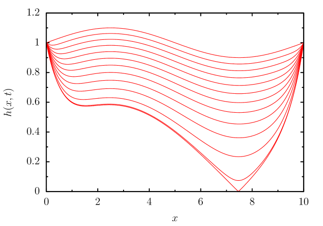
Figure 1: Successive profiles of the interface described by (25), with $\lambda=0.7>2/3$. The criterion (28) for unconditional stability is verified uniformly.

Close to pinch-off, (25) exhibits type-II self-similarity [6], characterized by the presence of logarithmic corrections to power law scaling. However, the minimum radius $h_{min}$ scales with a simple power law exponent of $1/2$. To test this, and to confirm stability of our scheme down to very small scales, we followed the solution until spatial resolution was lost. In Fig. 2, we show a doubly logarithmic plot of $h_{min}$ as a function of $t_{0}-t$, where $t_{0}$ is the singularity time. We determined $t_{0}$ by extrapolating $h_{min}(t)$ towards zero. The numerical solution is seen to exhibit the expected scaling down to the smallest resolvable scales, as illustrated in the inset.

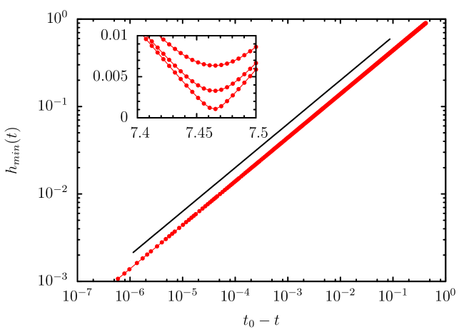
Figure 2: Minimum radius of the interface as a function of $t_{0}-t$, where $t_{0}$ is the pinch-off time. The full line corresponds to $(t_{0}-t)^{1/2}$. In the inset, we show a closeup of near the pinch point, plotting a profile every 10 time steps (but with adaptive time step).

To confirm that the method is indeed second-order accurate in time, we calculated the error as the $\infty-$norm of the difference between a numerical solution at a fixed time $t=0.4$, obtained with time step $\delta t=0.4\times 2^{-m}$ and the ”exact” solution obtained with the smallest time step $\delta t_{min}=0.4\times 2^{-16}$, divided by the maximum value of the solution :

$$\textrm{Error}=\frac{Max_{j}\left|f_{j}(\delta t_{min})-f_{j}(\delta t)\right|}{Max_{j}\left|f_{j}(\delta t_{min})\right|}.$$ (29)

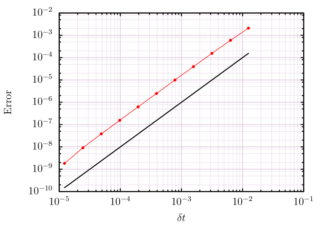
Figure 3: The maximum error (29) of the numerical solution of (25) at $t=0.4$, as a function of $\delta t$. The solid line corresponds to a quadratic dependence, which shows that the error using Richardson extrapolation scales like $\delta t^{2}$.

As seen in Fig. 3, the error scales indeed like $\delta t^{2}$, the same as expected for a fully implicit method, using for example the Crank-Nicolson scheme.

5 Hele-Shaw flow with surface tension

In the preceeding example, a fully implicit treatment of the right hand side of (25) would at least have been feasible [9], although our method simplifies the algorithm. By contrast, examples presented in [2] are much more challenging, in that the RHS is both nonlinear and non-local. We focus on the particular example of Hele-Shaw interface flow, whose spatial derivatives scale like $|k|^{3}$ in Fourier space, and thus lead to a very stiff system. While it is perfectly possible to stabilize the scheme using ordinary diffusion, according to our analysis of subsection 3.1, this would entail an increased time truncation error. Therefore, we use the Hilbert transform to construct a stabilizing term which is of third order in the spatial derivative, yet only takes $\mathcal{O}(N\log N)$ operations to calculate.

5.1 Equations

We consider an interface in a vertical Hele-Shaw cell, separating two viscous fluids with the same dynamic viscosity [2]. As heavy fluid falls, a slightly perturbed interface is deformed strongly by gravity, while surface tension assures regularity on small scales, as seen in Fig. 6 below. For simplicity, we assume the flow to be periodic in the horizontal direction.

The interface is discretized using marker points labeled with $\alpha$, which are advected according to :

$$\frac{\partial{\bf X}(\alpha)}{\partial t}=U{\bf n}+T{\bf s}.$$ (30)

Here ${\bf X}(\alpha)=(x,y)$ is the position vector, ${\bf n}=(-y_{\alpha}/s_{\alpha},x_{\alpha}/s_{\alpha})$ and ${\bf s}=(x_{\alpha}/s_{\alpha},y_{\alpha}/s_{\alpha})$ are the normal and tangential unit vectors, respectively. Hence $U=(u,v)\cdot{\bf n}$ and $T=(u,v)\cdot{\bf s}$ are the normal and tangential velocities, respectively. Since the evolution of a surface is determined only by its normal velocity, we can choose the tangential velocity of the marker points freely, in order to keep a reasonable distribution of points and avoid point clustering. The precise choice of the tangential velocity will be described later. For an unbounded interface, the complex velocity of marker points labeled with $\alpha$ is given by the Birkhoff–Rott integral [10]:

$$w(\alpha)=u(\alpha)-iv(\alpha)=\frac{1}{2\pi i}PV\int_{-\infty}^{+\infty}{\frac{\gamma(\alpha^{\prime},t)}{z(\alpha,t)-z(\alpha^{\prime},t)}d\alpha^{\prime}},$$ (31)

where $z(\alpha,t)=x+iy$. Here $\gamma$ is the vortex sheet strength at the interface. If the surface is periodic with period $1$ ($z(\alpha+2\pi)=z(\alpha)+1$), (31) can be written as an integral over the periodic domain $\alpha\in[0,2\pi]$ of the label:

$$u(\alpha)-iv(\alpha)=\frac{1}{2i}PV\int_{0}^{2\pi}{\gamma(\alpha^{\prime},t)\cot\left[\pi(z(\alpha,t)-z(\alpha^{\prime},t))\right]d\alpha^{\prime}},$$ (32)

where we have used the continued fraction representation of the cotangent [11] :

$$\pi\cot(\pi z)=\frac{1}{z}+2z\sum_{k=1}^{\infty}{\frac{1}{z^{2}-k^{2}}}.$$

For two fluids of equal viscosity, the vortex sheet strength $\gamma$ is given by [10] :

$$\gamma=S\kappa_{\alpha}-Ry_{\alpha},$$ (33)

where $\kappa$ is the mean curvature of the interface :

$$\kappa(\alpha)=\frac{x_{\alpha}y_{\alpha\alpha}-y_{\alpha}x_{\alpha\alpha}}{s_{\alpha}^{3}},\qquad\mathrm{with}\qquad s_{\alpha}=(x_{\alpha}^{2}+y_{\alpha}^{2})^{1/2}.$$ (34)

Here $S$ is the non-dimensional surface tension coefficient and $R$ is the non-dimensional gravity force. As an initial condition, we choose the same as the one used in [2], which corresponds to a slight modulation of a flat interface:

$$x(\alpha,0)=\alpha/2\pi,\quad y(\alpha,0)=0.01(\cos(\alpha)-\sin(3\alpha)).$$ (35)

To compute the complex Lagrangian velocity of the interface (32), we use the spectrally accurate alternate point discretization [12] :

$$u_{j}-iv_{j}\simeq-\frac{2\pi i}{N}\sum_{{l=0}\atop{j+l\;odd}}^{N-1}{\gamma_{l}\cot\left[\pi(z_{j}-z_{l})\right]}.$$ (36)

$\kappa_{\alpha}$ and $y_{\alpha}$ are computed at each time step using second-order centered finite differences, and $\alpha$ is defined by $\alpha(j)=2\pi j/N$, where $j\in[0,N]$ and $N$ is the number of points describing the periodic surface. Note that the numerical effort of evaluating (36) requires $\mathcal{O}(N^{2})$ operations, and thus will be the limiting factor of our algorithm. For the tangential velocity $T$, we use the same expression as [2], which is designed to avoid point clustering. For completeness, we describe the procedure in the Appendix.

5.2 Third-order stabilizing operator

It follows from (32) and (33), that the Hele-Shaw dynamics contains a stiff part which scales like $|k|^{3}$ in Fourier space [2]. As a result, we need to define a third-order operator to stabilize the equations. When the interface is described using marker points labeled with $\alpha$, the most natural choice of damping operating on the Cartesian coordinates $\left(x(\alpha),y(\alpha)\right)$ is :

$$\mathcal{D}\left[\left(x(\alpha),y(\alpha)\right)\right]=\left(\mathscr{H}(x_{\alpha\alpha\alpha}),\mathscr{H}(y_{\alpha\alpha\alpha})\right).$$ (37)

Here $\mathscr{H}$ is the Hilbert transform :

$$\mathscr{H}\left[f\right](\alpha)=\frac{1}{\pi}\int_{-\infty}^{+\infty}{\frac{f(\alpha^{\prime})}{\alpha-\alpha^{\prime}}d\alpha^{\prime}},$$

which satisfies :

$$\mathscr{H}\left[e^{ikx}\right]=-i\;\mathrm{sign}(k)\;e^{ikx},\qquad\mathscr{H}\left[1\right]=0.$$ (38)

Note that

$$R\mathcal{D}\left[\left(x(\alpha),y(\alpha)\right)\right]=\mathcal{D}R\left[\left(x(\alpha),y(\alpha)\right)\right],$$

where $R$ is an arbitrary rotation matrix. Thus the stabilizing terms share the same invariance under rotation as the original problem (30).

Using the first property (38), one notes that the scaling of the operators for a single mode $e^{ik\alpha}$ (in $x$ or $y$) is :

$$\mathcal{D}[e^{ik\alpha}]=-\left|k\right|^{3}e^{ik\alpha}.$$ (39)

Using the representation (39) in Fourier space, we can compute the stabilizing operators (37) in $\mathcal{O}(N\log N)$ operations with the aid of the Fast Fourier Transform [13], which leads to the following numerical algorithm.

First, the set of horizontal coordinates of the marker points has to be modified, such that $x^{\prime}_{j}$ is periodic:

$$x^{\prime}_{j}=x^{\prime}(\alpha(j))=x(\alpha(j))-j/N.$$

Now we are able to compute the discrete Fourier transform of $x^{\prime}_{j}$:

$$\hat{x}^{\prime}_{k} = \sum_{j=0}^{N-1}{x^{\prime}_{j}e^{-2i\pi jk/N}},$$ (40)

where $k=0,\dots,N-1$. Modes with $k>N/2$ correspond to negative wavenumbers of modulus $N-k$. The transforms of $y$, as well as the velocity components $u$ and $v$ are defined analogously. Each of these transforms can be performed using the Fast Fourier Transform, the velocity components at the old time step $n$ are computed from (36).

Now the discrete version of (30) becomes, including the stabilizing terms :

$$\frac{\hat{x}^{\prime n+1}_{k}-\hat{x}^{\prime n}_{k}}{\delta t} = \hat{u}_{k}^{n}-\lambda k^{3}\hat{x}^{\prime n+1}_{k}+\lambda k^{3}\hat{x}^{\prime n}_{k}$$ (41)

$$\frac{\hat{y}_{k}^{n+1}-\hat{y}_{k}^{n}}{\delta t} = \hat{v}_{k}^{n}-\lambda k^{3}\hat{y}_{k}^{n+1}+\lambda k^{3}\hat{y}_{k}^{n},$$ (42)

where $\hat{x}^{\prime}_{k}$ and $\hat{y}_{k}$ are complex numbers, and $k=0,\dots,N/2$. From equations (41) and (42), $\hat{x}^{\prime n+1}_{k}$ and $\hat{y}_{k}^{n+1}$ are found according to :

$$\hat{x}^{\prime n+1}_{k} = \hat{x}^{\prime n}_{k}+\frac{\hat{u}_{k}^{n}\;\delta t}{1+\lambda k^{3}\delta t}$$ (43)

$$\hat{y}_{k}^{n+1} = \hat{y}_{k}^{n}+\frac{\hat{v}_{k}^{n}\;\delta t}{1+\lambda k^{3}\delta t}.$$ (44)

For $k>N/2$, Fourier coefficients are found from $\hat{x}^{\prime n+1}_{k}=\left(\hat{x}^{\prime n+1}_{N-k}\right)^{*}$ and $\hat{y}^{n+1}_{k}=\left(\hat{y}^{n+1}_{N-k}\right)^{*}$. Finally, the inverse Fourier Transform of $\hat{x}^{\prime n+1}_{k}$ and $\hat{y}_{k}^{n+1}$ yields the components of $x$ and $y$ at the new time step:

$$x_{j}^{n+1} = \frac{1}{N}\sum_{k=0}^{N-1}{\hat{x}^{\prime n+1}_{k}e^{2i\pi jk/N}}+\frac{j}{N}$$ (45)

$$y_{j}^{n+1} = \frac{1}{N}\sum_{k=0}^{N-1}{\hat{y}_{k}^{n+1}e^{2i\pi jk/N}}.$$ (46)

The cost of this procedure represents a small effort compared to the evaluation of the velocities (36), which requires $\mathcal{O}(N^{2})$ operations.

5.3 von Neumann stability analysis

We are considering the amplification of small short-wavelength perturbations on the interface. In view of the rotational invariance of the system of equations, we can suppose an almost horizontal interface $0\leq x\leq 1$:

$$z_{j}=\frac{j}{N}+iy_{j},$$

where the $y_{j}$ are small and represent small perturbations. Then the linearization of (33) and (34) reads (keeping only the highest derivative):

$$\gamma_{j}^{n}=S\frac{\kappa^{n}_{j+1}-\kappa^{n}_{j-1}}{2\delta\alpha},\quad\kappa^{n}_{j}=(2\pi)^{2}\frac{y^{n}_{j+1}-2y^{n}_{j}+y^{n}_{j-1}}{\delta\alpha^{2}},$$

and the explicit part of the equation is, using (36):

$$\frac{y_{j}^{n+1}-y_{j}^{n}}{\delta t}=\frac{2\pi}{N}\sum_{{\ell=0}\atop{j+\ell\;odd}}^{N-1}{\gamma^{n}_{\ell}\cot\left[\frac{\pi}{N}(j-\ell)\right]}.$$ (47)

As before, we make the ansatz $y_{j}^{n}=\xi^{n}e^{ikj\delta\alpha}$, which yields

$$\gamma^{n}_{j}=2i\xi^{n}S\frac{(2\pi)^{2}}{\delta\alpha^{3}}\left(\cos\frac{2\pi k}{N}-1\right)\sin\frac{2\pi k}{N}e^{ikj\delta\alpha}.$$

Finally, using the discrete form of the Hilbert transform, we obtain [14]:

$$\frac{\xi-1}{\delta t}=2iS\frac{(2\pi)^{3}}{\delta\alpha^{3}}\left(\cos\frac{2\pi k}{N}-1\right)\sin\frac{2\pi k}{N}H_{k},$$ (48)

where

$$H_{k}=\left\{\begin{array}[]{l}-i/2\quad 1\leq k\leq N/2-1\\ 0\quad k=0,N/2\\ i/2\quad N/2+1\leq k\leq N-1\quad\;.\end{array}\right.$$

Thus for wavenumbers $1\leq k\leq N/2-1$, we can identify the coefficient $a$ in equation (5) as

$$a=SN^{3}\left(\cos\frac{2\pi k}{N}-1\right)\sin\frac{2\pi k}{N}.$$ (49)

On the other hand, $\hat{y}_{k}^{n}=N\xi^{n}$, so according to (41) and (42) we find

$$b=\lambda k^{3}.$$ (50)

The Richardson scheme will be stable if $b>2a/3$, which means that :

$$\lambda>\frac{2S}{3}\frac{N^{3}}{k^{3}}\left(\cos\frac{2\pi k}{N}-1\right)\sin\frac{2\pi k}{N},$$ (51)

a condition which needs to be satisfied for all $k\leq N/2-1$ to guarantee unconditional stability. The maximum of the right hand side of (51) is $(2\pi)^{3}/2$, which is in fact achieved in the limit of small $k$, as verified numerically below. Thus the stability criterion becomes

$$\lambda>\frac{S(2\pi)^{3}}{3}\approx 82.7S.$$ (52)

So far our calculation was based on an interface of length 1, while the markers run from $0$ to $2\pi$; this is the origin of the factor $(2\pi)^{3}=s_{\alpha}^{-3}$ in (52). As the interface is stretched during the computation, $s_{\alpha}$ increases and the stability constraint becomes less stringent:

$$\lambda>\frac{S}{3s_{\alpha}^{3}}.$$ (53)

To achieve an optimal result, one could choose $\lambda$ as a function of space and time, depending on the local value of $s_{\alpha}$. For simplicity, in the computations reported below, we choose $\lambda$ to be time dependent only, based on the minimum value of $s_{\alpha}$ over space, which is estimated as

$$s_{\alpha}\approx\frac{\delta s_{min}N}{2\pi},$$

where $\delta s_{min}$ is the minimum spatial distance between grid points.

5.4 Numerical results

The spatial convergence of our method has been tested by comparing to a ”true” solution, computed using a fine grid with $N=2^{13}$. Then, the relative error to this solution is computed for the vertical velocity and the vortex sheet strength at $t=0$, for smaller values of $N$. A relative error of the whole code is also computed for the height of the interface at $t=0.01$. Figure 4 presents these results, plotted against the initial $\delta x$, together with a power fit, that proves the spatial convergence to scale like $\delta x^{2}$.

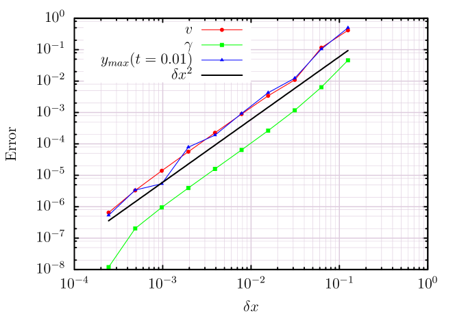
Figure 4: Spatial truncation errors, as a function of the initial uniform $\delta x$. The “true” solution is obtained with the finest grid, with $2^{13}$ points. The red circles correspond to the relative error on the vertical velocity at $t=0$, computed using equation (32). The green squares correspond to the relative error on the vortex sheet strength $\gamma$ at $t=0$, computed using equation (33). The blue triangles correspond to the relative error on the maximum value of $y$ at $t=0.01$. The solid line shows that all these relative errors scale like $\delta x^{2}$.

To probe the damping of any numerical instability by the scheme (43),(44), we recorded the spectra of a solution close to a horizontal interface, with a very small perturbation added to it. The spectra are shown every 30 time steps, starting from the initial condition. If $\lambda$ is chosen slightly larger than the boundary (52), the spectrum remains flat and free of unphysical growth for large wave numbers, as seen on the right of Fig. 5. If on the other hand $\lambda$ is chosen somewhat smaller, numerical instability first occurs toward the small wavenumber end of the spectrum, as seen on the left of Fig. 5. This is in agreement with (51), which shows that the stability condition is first violated for small $k$.

Although this might seem unusual at first, the observed growth for small $k$ is simply a result of our choice of damping, which slightly emphasizes large wavenumbers relative to smaller ones. Had we chosen to implement (37) using finite differencing for $x_{\alpha\alpha\alpha}$ and $y_{\alpha\alpha\alpha}$, and only performing the Hilbert transform in Fourier space, the critical value of $\lambda$ would have been independent of $k$.

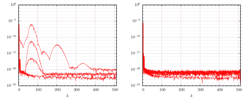
Figure 5: Evolution of the amplitude spectrum of the vertical displacement $y_{j}^{n}$ for two different values of $\lambda$ : $\lambda=70\;S$ on the left, $\lambda=85\;S$ on the right. The initial condition for both these computations is the same as (35), except that the initial amplitude is $10^{-6}$. The left computation becomes unstable for $t\gtrsim 3\times 10^{-3}$, whereas the right one remains stable. In both cases, $1024$ points have been used and the time step is $\delta t=3.125\times 10^{-5}$. Spectra are shown every 30 time steps.

In Fig. 6, we compare our results to the long time run of Hele-Shaw dynamics, presented as a bench mark for the methods developed in [2]. Our computations are shown on left at the times indicated, those of [2] are shown on the right at identical times. We have chosen the same physical parameters, as well as the same spatial resolution ($N=2048$), and time step $\delta t=3.125\times 10^{-5}$. Periodic boundary conditions apply in the $x$-direction. No filtering was applied to our data, and no sign of instability could be observed throughout the highly non-linear evolution of the interface. As a consequence of the interplay between gravitational instability and surface tension, long wavelength perturbations are amplified first. Subsequently, the interface deforms into a highly contorted shape consisting of long necks bounded by rounded fluid blobs. In several places, and as highlighted in the last panel, fluid necks come close to pinch-off, and small scale structure is generated.

The results of the two computations are indistinguishable, except for the last panel, in which a closeup is shown. To investigate the source of the remaining discrepancy, we have repeated our computation at twice and four times the original spatial resolution, the results of which are shown in the left panel of Fig. 7. The right panel shows the original computation by [2], with $N=2048$. It is seen that to achieve convergence on the scale of the closeup, about $N=4096$ grid points are needed, which yields a result close to that for $N=8192$. Taking the highest resolution result as a reference, it is seen that our numerical scheme performs at least as well as the original scheme of [2].

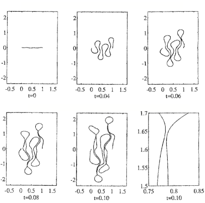
Figure 6: The instability of a Hele-Shaw interface with initial conditions (35), evolving according to (30), (32),(33), with parameters $S=0.1$, $R=-50$. In our computation ((a), left six panels), we have used $N=2048$ points, and $\delta t=3.125\times 10^{-5}$. The constant $\lambda$ was chosen according to $\lambda=0.35\;S(2\pi/N\delta s_{min})^{3}$, which satisfies the stability constraint (53). For comparison, we show the results of the original computation [2] ((b), right six panels), obtained for the same physical parameters, and using the same number of grid points and time step. Differences between the two calculations are visible in the closeup of the last panel only.

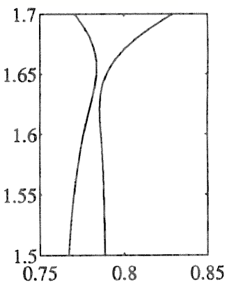
Figure 7: Comparison between our result (a) and the result presented in [2] (b), for the bottom right panel in Fig. 6. The solid curves correspond to $N=2048$ grid points, the dashed curve to $N=4096$ and the dotted curve to $N=8192$.

6 Application to Kuramoto-Sivashinsky equation

The final test of our method treats the Kuramoto–Sivashinsky equation [15], which contains fourth-order derivatives:

$$\frac{\partial u}{\partial t}=-u\frac{\partial u}{\partial x}-\frac{\partial^{2}u}{\partial x^{2}}-\frac{\partial^{4}u}{\partial x^{4}},$$ (54)

where all coefficients have been normalized to unity. The second-order term acts as an energy source and has a destabilizing effect, the nonlinear term transfers energy from low to high wavenumbers, while the fourth-order term removes the energy on small scales. The Kuramoto–Sivashinsky equation is known to exhibit spatio-temporal chaos, so the main interest lies in predicting the statistical properties of solutions. An accurate method for solving (54) is described in [16], where it is solved on the periodic domain $x\in[0,32\pi]$, with the initial condition :

$$u(x,t=0)=\cos\left(\frac{x}{16}\right)\left(1+\sin\left(\frac{x}{16}\right)\right).$$ (55)

We want to use (54) to illustrate the flexibility of our method, using a lower order term to stabilize the algorithm. Namely, we use $\lambda u_{xx}$, with $\lambda$ chosen in order to counteract the effect of $-u_{xxxx}$. We show that while this is certainly not the method of choice to solve this equation, it is sufficiently accurate to represent the statistics of the solution.

6.1 Numerical scheme

Equation (54) is discretized on a regular grid, using centered finite differences :

$$\frac{u_{j}^{n+1}-u_{j}^{n}}{\delta t}=-u_{j}^{n}\frac{u_{j+1}^{n}-u_{j-1}^{n}}{2\delta x}-\frac{u_{j-1}^{n}-2u_{j}^{n}+u_{j+1}^{n}}{\delta x^{2}}-\frac{u_{j-2}^{n}-4u_{j-1}^{n}+6u_{j}^{n}-4u_{j+1}^{n}+u_{j+2}^{n}}{\delta x^{4}}$$

$$-\lambda\frac{u_{j-1}^{n}-2u_{j}^{n}+u_{j+1}^{n}}{\delta x^{2}}+\lambda\frac{u_{j-1}^{n+1}-2u_{j}^{n+1}+u_{j+1}^{n+1}}{\delta x^{2}},$$ (56)

where $\lambda$ has to be chosen such that the method is stable.

6.2 Von Neumann stability analysis and numerical results

In order to find the right value of $\lambda$ for the scheme to be stable, we only need to consider the fourth-order derivative in the equation, which is the stiff term to be stabilized. As before, inserting $u_{j}^{n}=\xi^{n}e^{ikj\delta x}$ into (56), and retaining only $-u_{xxxx}$ from the Kuramoto–Sivashinsky equation, we obtain after simplification :

$$\frac{\xi-1}{\delta t}=-\frac{2}{\delta x^{4}}\left(\cos(2k\delta x)-4\cos(k\delta x)+3\right)+\frac{2\lambda}{\delta x^{2}}(\xi-1)\left(\cos(k\delta x)-1\right).$$ (57)

Again, we can identify coefficients $a$ and $b$ from equation (5) and obtain :

$$a=\frac{2}{\delta x^{4}}\left(\cos(2k\delta x)-4\cos(k\delta x)+3\right)\quad\mathrm{and}\quad b=\frac{2\lambda}{\delta x^{2}}\left(1-\cos(k\delta x)\right),$$ (58)

so that unconditional stability is guaranteed if

$$\lambda>\frac{2}{3\delta x^{2}}\frac{\cos(2k\delta x)-4\cos(k\delta x)+3}{1-\cos(k\delta x)}.$$

The maximum value of the right hand side occurs for the largest wave number $k_{max}=\pi/\delta x$, and the stability constraint becomes

$$\lambda>\frac{8}{3\delta x^{2}}.$$ (59)

We have chosen $\lambda=3/\delta x^{2}$ for our computations, so stability is assured regardless of the time step. However, according to the analysis of subsection 3.1, the fact that we are using a lower order operator for stabilization leads to a larger time truncation error than a fully implicit second order method would have. If we use (24) for an estimate of the required time step, we obtain

$$\delta t\simeq\frac{3\delta x^{4}}{8}\left(\frac{\Delta}{\delta x}\right)^{2}.$$ (60)

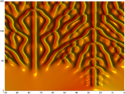
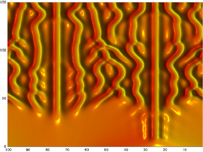
Figure 8: Solution of (54) with initial conditions (55). The horizontal axis represents the space variable, and the vertical axis time. On the left we show our calculation with $N=512$ grid points and $\delta t=0.014$, with $\lambda=3/\delta x^{2}$. For comparison, we show the computation of [16] on the right, which uses $128$ grid points and a time step $\delta t=1/4$.

In Fig. 8 we present a comparison of our computation (left) with the results of the high-resolution code given in [16] (right) as a reference. This code is of fourth order in both space and time, and we have confirmed that for $N=128$ and $\delta t=1/4$, the solution is represented accurately over the entire time interval shown in the figure. Since our code is only of second order in space, we have chosen $N=512$, which gives a spatial resolution of $\delta x\simeq 0.196$. Estimating the smallest relevant physical scale as $\Delta\simeq 1\simeq 5\delta x$, (60) yields $\delta t=1.4\times 10^{-2}$ as the time step. Note that this is 75 times larger than the minimum explicit time step $\delta t_{E}=\delta x^{4}/8$ required to stabilize the fourth-order operator.

We have used $\delta t=1.4\times 10^{-2}$ to produce Fig. 8 (left). Although the two solutions eventually evolve differently, it appears that their essential features are quite similar. It is important to reiterate that our purpose is not to compete with the fourth-order scheme of [16], but rather to demonstrate that we can stabilize a fourth-order PDE with a second-order operator, without destroying the statistical properties of the solution.

7 Conclusions

In this paper, we take a new look at the problem of stiffness, which leads to numerical instability in many equations of interest in physics. It is well established that a PDE can be split into several parts, some of which are treated explicitly, while only the stiff part is treated implicitly [17]. However, the realization of such a split may require great ingenuity [2], and has to be performed on a case-by-case basis. Moreover, the resulting implicit calculation may still require elaborate techniques.

We demonstrate a way around this problem by showing that any explicit algorithm can be stabilized using expressions foreign to the original equation. This implies a huge freedom in choosing a term which is both conceptually simple and inexpensive to invert numerically. In particular, the stabilizing does not need to represent a differential operator, nor does it need to have a physical meaning. Since the stiffness comes from short-wavelength modes on the scale of the numerical grid, we only require the stabilizing part to approximate the true operator in the short wavelength limit.

We note that although in this paper we were concerned mostly with uniform grids, this is by no means necessary, as stability criteria such as (28) or (53) are local. If the grid spacing varies, this can be accounted for by allowing $\lambda$ to vary in space as well as in time. A possibility we have not explored yet is to choose $\lambda$ adaptively. At the moment, the right choice of $\lambda$ requires some analysis of the high wavenumber behavior of the equation. An appropriate algorithm might be able to adjust to the optimal value of $\lambda$ automatically, which in general will be spatially non-uniform. Finally, the feasibility of our scheme in two space dimensions has already been demonstrated [3].

Appendix A Choice of tangential velocity

The tangential velocity of the interface is chosen such that the ratio of the distance between two successive points to the total length of the interface is conserved in time :

$$s_{\alpha}(\alpha,t)=R(\alpha)L(t)=R(\alpha)\int_{0}^{2\pi}{s_{\alpha^{\prime}}d\alpha^{\prime}},$$ (61)

where $\alpha$ is a marker label, $s(\alpha,t)$ is the arclength, $L(t)$ is the total length of the interface and $R(\alpha)$ is such that :

$$\int_{0}^{2\pi}{R(\alpha)}d\alpha=1.$$

We choose the tangential velocity such that $R(\alpha)$ does not change in time. Taking the time derivative of

$$s_{\alpha}=\sqrt{x_{\alpha}^{2}+y_{\alpha}^{2}}$$

and using the advection equation (30), one finds that

$$s_{\alpha t}=T_{\alpha}-\theta_{\alpha}U,$$ (62)

where $\theta$ is the angle between the local tangent and the $x$ axis.

Integrating equation (62) over $\alpha$ and using the time-derivative of equation (61) together with the fact that ${\displaystyle\int_{0}^{2\pi}{T_{\alpha^{\prime}}d\alpha^{\prime}}=0}$, one finally obtains :

$$T(\alpha,t)=T(0,t)+\int_{0}^{\alpha}{\theta_{\alpha^{\prime}}Ud\alpha^{\prime}}-\int_{0}^{\alpha}{R(\alpha^{\prime})d\alpha^{\prime}}\int_{0}^{2\pi}{\theta_{\alpha^{\prime}}Ud\alpha^{\prime}}.$$ (63)

References

- Mullins [1957] W. W. Mullins, Theory of thermal grooving, J. Appl. Phys. 28 (1957) 333.
- Hou et al. [1994] T. Hou, J. Lowengrub, M. Shelley, Removing the stiffness from interfacial flows with surface tension, J. Comp. Physics 114 (1994) 312–338.
- Douglas Jr. and Dupont [1971] J. Douglas Jr., T. F. Dupont, Alternating-direction galerkin methods on rectangles, in: B. Hubbard (Ed.), Numerical Solution of Partial Differential Equations II, Academic Press, 1971, pp. 133–214.
- Press [2007] W. Press, Numerical recipes : the art of scientific computing, Cambridge University Press, Cambridge, UK New York, 2007.
- Richtmyer and Morton [1967] R. D. Richtmyer, K. W. Morton, Difference methods for initial-value problems, Interscience, 1967.
- Eggers and Fontelos [2009] J. Eggers, M. A. Fontelos, The role of self-similarity in singularities of partial differential equations, Nonlinearity 22 (2009) R1.
- Ishiguro et al. [2007] R. Ishiguro, F. Graner, E. Rolley, S. Balibar, J. Eggers, Dripping of a crystal, Phys. Rev. E 75 (2007) 041606.
- Dziuk and Kawohl [1991] G. Dziuk, B. Kawohl, On rotationally symmetric mean curvature flow, J. Differential Equations 93 (1991) 142.
- Bernoff et al. [1998] A. J. Bernoff, A. L. Bertozzi, T. P. Witelski, Axisymmetric surface diffusion: Dynamics and stability of self-similar pinch-off, J. Stat. Phys. 93 (1998) 725–776.
- Majda and Bertozzi [2002] A. J. Majda, A. L. Bertozzi, Vorticity and Incompressible Flow, Cambridge University Press, Cambridge, 2002.
- Carrier et al. [1966] G. F. Carrier, M. Krook, C. E. Pearson, Functions of a complex variable, McGraw-Hill, New York, 1966.
- Shelley [1992] M. Shelley, A study of singularity formation in vortex sheet motion by a spectrally accurate vortex method, J. Fluid Mech. 244 (1992) 493.
- Frigo and Johnson [2005] M. Frigo, S. G. Johnson, The design and implementation of FFTW3, Proceedings of the IEEE 93 (2005) 216–231. Special issue on “Program Generation, Optimization, and Platform Adaptation”.
- Čížek [1970] V. Čížek, Discrete Hilbert transform, IEEE Trans. Audio Electroacoust. 18 (1970) 340.
- Cross and Hohenberg [1993] M. C. Cross, P. C. Hohenberg, Pattern formation outside of equilibrium, Rev. Mod. Phys. 65 (1993) 851–1112.
- Kassam and Trefethen [2005] A.-K. Kassam, L. Trefethen, Fourth-order time-stepping for stiff pdes, SIAM J. Sci. Comput. 26 (2005) 1214–1233.
- Ascher et al. [1995] U. M. Ascher, S. J. Ruuth, B. T. R. Wetton, Implicit-explicit methods for time-dependent partial differential equations, SIAM J. Numer. Amal. 32 (1995) 797.