Generalized effective hamiltonian for graphene under non-uniform strain

Abstract

We use a symmetry approach to construct a systematic derivative expansion of the low energy effective Hamiltonian modifying the continuum Dirac description of graphene in the presence of non-uniform elastic deformations. We extract all experimentally relevant terms and describe their physical significance. Among them there is a new gap-opening term that describes the Zeeman coupling of the elastic pseudomagnetic field and the pseudospin. We determine the value of the couplings using a generalized tight binding model.

I Introduction

The effects of lattice deformations on the electronic properties of graphene has been a topic of interest since the very early days due to the observation of ripples in suspended samples Meyer et al. (2007). Later on, the subject acquired a new dimension after the recognition of the extraordinary mechanical properties of the material Lee et al. (2009) and the capability of tailoring the samples to exploit the interplay of mechanical and electronic properties Kim et al. (2009); Tomori et al. (2011). The successful description of the influence of elastic deformations on the electronic excitations in terms of “elastic gauge fields” Suzuura and Ando (2002); Guinea et al. (2008a); Vozmediano et al. (2010) has been extensively used in the proposals of strain engineering in real Decker et al. (2011) and synthetic samples Gomes et al. (2012). The interest in the effective low energy Hamiltonian of deformed graphene has been reactivated recently based on the apparent discrepancy between the lattice description – tight binding (TB) approximation and subsequent continuum limit – and an alternative geometric approach using the formalism of quantum field theory in curved spaces de Juan et al. (2007, 2012). There have also been recent claims of the emergence of new gauge fields in the standard TB approach originating from the deformation of the lattice vectors Kitt et al. (2012, 2013); de Juan et al. (2013).

Given the rapid progress in this field one obvious question is, have we considered all possible effects of strain on the electronic properties of graphene or are we missing some? This is a crucial question, as particular models and approximations tend to capture specific features of the physics and, as a consequence, are likely to miss other aspects. We may answer this question by using group theory techniques to generate all possible interactions respecting the symmetries of the system, and then try to find a model to estimate the values of their couplings.

The idea of constructing effective actions for physical systems based solely on symmetry considerations has a long tradition both in quantum field theory (QFT) Ramond (1997) and condensed matter physics, and lies at the hearth of the Landau Fermi liquid theory of metals Landau (1957). The Dirac description of the low energy electronic excitations of graphene in the continuum limit is rooted in the symmetries of the underlying honeycomb lattice, as has been known for a long time Slonczewski and Weiss (1958). The symmetry approach has been applied to the particular problem of strained graphene, for example, in refs. Mañes, 2007; Winkler and Zulicke, 2010; Ferone et al., 2011; Linnik, 2012; Cabra et al., 2013. A highly detailed symmetry construction has been used in ref. Basko, 2008 to extract the low energy Hamiltonian affecting the Raman responses in graphene and, more recently, to explore the influence of the flexural modes on the spin–orbit coupling Ferone et al. (2011); Ochoa et al. (2012).

While many previous studies have concentrated on uniform strains, important effects such as the emergence of pseudomagnetic fields Guinea et al. (2010a) and the new vector fields de Juan et al. (2007, 2012) responsible for pseudospin precession de Juan et al. (2013) require the presence of non-uniform strain. Under non-uniform strain, new interaction terms arise which depend not just on the strain components, but also on their derivatives. In this work we apply standard symmetry based methods to construct a low energy effective hamiltonian for graphene in the presence of non-uniform elastic deformations. In order to accomplish this, we set up a systematic expansion in derivatives of the strain and use group theory techniques to guarantee that all the symmetry allowed terms up to a given order are included. Next we compute the coefficients of the most relevant terms –those which will affect the experiments – within a generalized tight binding approximation, which sheds light on the physical origin and significance of the various interactions in the effective hamiltonian. Those terms which do not involve derivatives of the strain have been already discussed in the literature, but among the new interactions predicted by the symmetry approach there is one that opens a gap and represents the Zeeman coupling between the elastic pseudomagnetic field and pseudospin. We discuss the physical strength of this coupling within the generalized tight binding model and analyze some physical consequences.

The article is organized as follows. In Sec. II we outline the properties of the graphene system relevant to our symmetry analysis and set up a systematic expansion in the derivatives of the strain tensor. Sec. III summarizes the results of the symmetry analysis and contains a description of all the possible terms in the low energy Hamiltonian for deformed graphene with at most one derivative. The effects of including higher derivatives are explored in Subsec. III.2. In Sec. IV we introduce a generalized tight binding model which is used to compute the coefficients of the low energy Hamiltonian both for in–plane strains and out–of–plane distortions (IV.1). We also consider the geometric terms due to frame effects (IV.2) and discuss some physical implications of the new gap opening term (IV.3). In Sec. V we summarize our work and consider possible extensions.

II Effective hamiltonian, derivative expansion and symmetries

In this paper we consider a systematic expansion of the hamiltonian in derivatives of the the electron field and the strain tensor 

$$u_{ij}=\frac{1}{2}(\partial_{i}\xi_{j}+\partial_{j}\xi_{i}+\partial_{i}h\partial_{j}h)\;\;\;,\;\;\;i,j=x,y,$$ (1)

where $\xi_{i}$ and $h$ are horizontal and vertical displacements respectively. This makes sense in the presence of elastic deformations, where each new derivative of the strain is expected to be suppressed by a factor of order $\mathcal{O}(a/\lambda)$, where $\lambda$ is the wavelength of the deformation and $a$ is the lattice constant. As we are interested in a continuum low energy approximation where electrons behave like Dirac fermions, we will restrict ourselves to terms that are at most linear in the electron momentum $k$, where $k$ is measured with respect to a Fermi point. Moreover, we will assume that the system is within the domain of applicability of standard linear elasticity theory and consider only terms linear in the strain tensor. Thus the effective hamiltonian will be a function of the electron fields $\psi$ and $\psi^{\dagger}$, the strain $u_{ij}$ and their derivatives. Each order in the derivative expansion will be characterized by $(n_{q},n_{k})$, where $n_{q}$ and $n_{k}$ count the order of the derivatives of the strain and electron fields respectively. Possible extensions of this approach to include nonlinear contributions and optical modes will be discussed in Sect. V

$(n_{q},n_{k})$	$(0,0)$	$(0,1)$	$(1,0)$	$(1,1)$	$(2,0)$
$\openone$	1	1	0	0	2
$\{\sigma_{x},\sigma_{y}\}$	1	2	0	0	3
$\sigma_{z}$	0	0	1	2	0

Table 1: Number of independent hermitian invariants linear in $u_{ij}$ at order $(n_{q},n_{k})$ in the derivative expansion, containing the four $2\times 2$ hermitian matrices $\{\openone,\vec{\sigma}\}$. For each of these invariants another one can be constructed through the substitution $u_{ij}\rightarrow\partial_{i}h\partial_{j}h$.

Any valid effective hamiltonian must respect all the symmetries of the system. In the case of graphene, these include the point group $D_{6h}$ of the honeycomb lattice . $D_{6h}$ consists of $24$ symmetry operations, and one of them is reflection by the horizontal plane $\sigma_{h}$. A first simplification is afforded by the fact that all the ingredients in the effective hamiltonian are invariant under reflection by $\sigma_{h}$. More concretely, electron fields are combinations of $p_{z}$ orbitals which are odd under $\sigma_{h}$, but only bilinears in the electron field are allowed in the hamiltonian and these are obviously even. Similarly, vertical atomic displacements $h$ are odd under $\sigma_{h}$, but only the combinations $(\partial_{i}h)(\partial_{j}h)$ enter the hamiltonian and these are even. As a consequence, we may ignore $\sigma_{h}$ as a symmetry and consider $C_{6v}$ instead of $D_{6h}$. $C_{6v}$ has only $12$ elements, which include rotations by multiples of $\pi/3$ around the $OZ$ axis and reflections by six vertical planes.

As is well known Castro Neto et al. (2009) the Fermi surface of the system at half filling consists of six Dirac points located at the corners of the Brillouin zone in momentum space. Only two are non–equivalent, and can be chosen at opposite corners, $K_{2}=-K_{1}$. We will study the case where there are no interactions relating the two Fermi points and analyze each of them independently. Then the low energy description of the electronic excitations around these points is governed by two Dirac Hamiltonians related by time reversal. This is the relevant situation for long wavelength elastic deformations, and in this case the Dirac points are protected against gap opening by smooth deformations respecting inversion and time reversal symmetryMañes et al. (2007). Then symmetry allowed interactions around $K_{1}$ must be invariant only under the elements of $C_{6v}$ which leave $K_{1}$ invariant. This is known as the little point group Bradley and Cracknell (2010) of $K_{1}$, which is given by $C_{3v}$. As reviewed in Appendix A, $C_{3v}$ is a subgroup of $C_{6v}$ with only $6$ elements: rotations by multiples of $2\pi/3$ around the $OZ$ axis and reflections by three vertical planes. Besides the little point group $C_{3v}$, $K_{1}$ is also invariant under the combined operation $C_{2}\theta$, where $C_{2}$ is a rotation by $\pi$ around the $OZ$ axis and $\theta$ is time reversal. Once a hamiltonian respecting $C_{3v}$ and $C_{2}\theta$ has been constructed around $K_{1}$, time-reversal symmetry, which takes $K_{1}$ into $K_{2}$, can be used to obtain the hamiltonian at $K_{2}$. This ensures that the total hamiltonian, which is the sum of the two hamiltonians around $K_{1}$ and $K_{2}$, respects all the symmetries of the system.

Once we know the set of symmetries to be respected by the interaction terms, the next step is to classify the relevant magnitudes according to their transformation properties. The result is shown in Table 8 in Appendix A, where the relevant objects are assigned irreducible representations of the little point group $C_{3v}$ and their behaviour under $C_{2}\theta$ is indicated. Then one can use Eq. (21) to determine the number of independent hermitian invariant terms at each derivative order $(n_{q},n_{k})$ (see Table 1). This crucial step guarantees that all symmetry compatible interactions are taken into account. Then standard group theory techniques are used to construct all the symmetry allowed interactions.

III Symmetry-allowed terms in the Effective hamiltonian

III.1 Effective Hamiltonian to first derivative order

$H_{i}$	$(n_{q},n_{k})$	Interaction term	Physical interpretation	$K_{2}$
$H_{1}$	(0,0)	$(u_{xx}+u_{yy})\openone$	Position-dependent electrostatic pseudopotential	$+$
$H_{2}$	(0,0)	$(u_{xx}-u_{yy})\sigma_{x}-2u_{xy}\sigma_{y}$	Dirac cone shift or U(1) pseudogauge field $(A_{x},A_{y})$	$-$
$H_{3}$	(0,1)	$\big{[}(u_{xx}-u_{yy})k_{x}-2u_{xy}k_{y}\big{]}\openone$	Dirac cone tilt	$-$
$H_{4}$	(0,1)	$(u_{xx}+u_{yy})(\sigma_{x}k_{x}+\sigma_{y}k_{y})$	Isotropic position-dependent Fermi velocity	$+$
$H_{5}$	(0,1)	$u_{ij}\sigma_{i}k_{j}\;\;;\;\;i,j=x,y$	Anisotropic position-dependent Fermi velocity	$+$
$H_{6}$	(1,0)	$\;\;\;\;\big{[}\partial_{y}(u_{xx}-u_{yy})+2\partial_{x}u_{xy}\big{]}\mathbf{\sigma}_{z}\;\;\;\;$	Gap opening by non-uniform strain	$-$

Table 2: Effective low-energy electron-strain interactions allowed by symmetry.

The results of following the procedure outlined above and detailed in Appendix A may be summarized in an effective hamiltonian which contains all the symmetry allowed interactions to first derivative order, i.e., for $n_{q}+n_{k}\leq 1$. This is given by

$$H=H_{0}+\sum_{i=1}^{6}a_{i}H_{i}+\sum_{i=1}^{6}\tilde{a}_{i}\tilde{H}_{i},$$ (2)

where $H_{0}=v_{F}(\sigma_{x}k_{x}+\sigma_{y}k_{y})$ and the terms $H_{i}$ are given in Table 2. The terms $\tilde{H}_{i}$ are obtained from those in Table 2 through the substitution $u_{ij}\rightarrow\partial_{i}h\partial_{j}h$, where $h$ is the vertical displacement. The reason for the appearance of the extra terms $\tilde{H}_{i}$ in the hamiltonian is that $\partial_{i}h\partial_{j}h$ transforms exactly like $u_{ij}$ under all the symmetries of the system. Thus for each invariant written in terms of $u_{ij}$ another one exists with $u_{ij}$ replaced by $\partial_{i}h\partial_{j}h$, and the coefficients of $H_{i}$ and $\tilde{H}_{i}$ have to be determined independently. This will be done in the next Section and, for the time being, we will refer to the more familiar $H_{i}$. At the end of this Section we will argue that the effective hamiltonian (2) probably captures all the experimentally relevant effects due to non-uniform strain.

Eq.(2) gives the form of the first-quantized hamiltonian. The corresponding second-quantized hamiltonian operator is given by $\hat{H}\!=\!\int d^{2}x\,\psi^{\dagger}H\psi$, where the symmetric convention for the derivatives acting on the electron fields is understood, i.e., $\psi^{\dagger}k_{i}\psi\!\rightarrow\!-i/2(\psi^{\dagger}\overleftrightarrow{\partial_{i}}\psi)\!\equiv\!-i/2(\psi^{\dagger}\partial_{i}\psi-\partial_{i}\psi^{\dagger}\psi)$. For instance, $\hat{H}_{5}$ is given by

$$\hat{H}_{5}=-\frac{i}{2}\int d^{2}x\,u_{ij}(\psi^{\dagger}\sigma_{i}\overleftrightarrow{\partial_{j}}\psi),$$ (3)

where $\partial_{j}$ acts only on the electron fields. The advantage of using the symmetric derivative convention is that any real expression in the electron momentum $k$, the strain (and its derivatives) and a hermitian matrix will automatically give rise to a second-quantized hermitian operator. This simplifies the counting and construction of hermitian invariants. In this regard, it is important to realize that $(n_{q},n_{k})$ in Table 2 gives the orders of the derivatives when terms are written with the symmetric convention. See also comments around Eq. (5) below.

Table 2 displays all the hermitian, symmetry-allowed terms of given orders $(n_{q},n_{k})$ in the derivatives of the electron fields ($n_{k}$) and strain ($n_{q}$), as indicated in the second column. The remaining columns give their physical interpretation and the relative sign of the couplings at the two non-equivalent Dirac points. In what follows we will comment briefly on the physical significance of the various terms which, with the exception of $H_{6}$, have already been given  in refs. Winkler and Zulicke, 2010; Linnik, 2012:

• $H_{1}=(u_{xx}+u_{yy})\openone$: This term has the form of a scalar potential $\Phi\sim u_{xx}+u_{yy}$ and was already described in ref. Suzuura and Ando, 2002, where the coupling strength was estimated to be of order 4 eV for single layer graphene. Its physical consequences have been explored in ref. Low et al., 2011.

• $H_{2}=(u_{xx}-u_{yy})\sigma_{x}-2u_{xy}\sigma_{y}$: Dirac cone shift in momentum space or $U(1)$ pseudogauge field $(A_{x},A_{y})\sim(u_{xx}-u_{yy},-2u_{xy})$. This term corresponds to the well known elastic pseudogauge fields of the standard tight binding approach. It has been used in the literature to propose all kinds of strain engineering and to fit experimental measurements of very intense pseudomagnetic fields in corrugated graphene samples Vozmediano et al. (2010). It has also been used to explain data in artificial graphene Gomes et al. (2012).

• $H_{3}=\big{[}(u_{xx}-u_{yy})k_{x}-2u_{xy}k_{y}\big{]}\openone$: Dirac cone tilt. This term appears naturally in the description of the two dimensional organic superconductors Kobayashi et al. (2007) which are described by anisotropic Dirac fermions. It also arises when applying uniaxial strain in the zigzag direction, a situation that has been discussed at length in the literature Goerbig et al. (2008); Wunsch et al. (2008); Montambaux et al. (2009); Choi et al. (2010).

• $H_{4}=(u_{xx}+u_{yy})(\sigma_{x}k_{x}+\sigma_{y}k_{y})$: Isotropic position-dependent Fermi velocity de Juan et al. (2012).

• $H_{5}=u_{ij}\sigma_{i}k_{j}\;\;;\;\;i,j=x,y$: Anisotropic position-dependent Fermi velocity de Juan et al. (2012). This term, together with $H_{4}$, was predicted to arise within the geometric modeling of graphene based on techniques of quantum field theory in curved space de Juan et al. (2007). It was later obtained in a tight binding model by expanding the low energy hamiltonian to linear order in $q$ and $\xi$ de Juan et al. (2012, 2013). It comes together with a new vector field $\Gamma_{i}$ that will be discussed below. Since the Fermi velocity is the most important parameter in the graphene physics, this term affects all the experiments and will induce extra spatial anisotropies in strained samples near the Dirac point Guinea et al. (2008b); Brey and Palacios (2008); Zhang et al. (2009); Gazit (2009); Gibertini et al. (2012); Pellegrino et al. (2011).

• $H_{6}=\big{[}\partial_{y}(u_{xx}-u_{yy})+2\partial_{x}u_{xy}\big{]}\mathbf{\sigma}_{z}$: This is a very interesting term that suggests a new gap-opening mechanism that has not been noticed previously. It can be seen as the Zeeman coupling of pseudospin to the associated pseudomagnetic field $B_{z}=\partial_{x}A_{y}-\partial_{y}A_{x}$Zhang et al. (2013). The magnitude of this new gap will be estimated in Subsec. IV.3 where we will explore its physical implications.

• To first order in the derivative expansion we can also construct an invariant involving the antisymmetric derivative of the displacement vector $\omega=\partial_{x}\xi_{y}-\partial_{y}\xi_{x}$:

  $$\omega(k_{x}\sigma_{y}-k_{y}\sigma_{x})=\omega\epsilon_{ij}k_{i}\sigma_{j},$$ (4)

  but, as shown in Ref. de Juan et al., 2013, it can be eliminated by a local rotation of the pseudospinor $\psi\rightarrow\exp(-\frac{i}{2}\omega\sigma_{z})\,\psi$. Thus the effective hamiltonian (2) does not depend on $\omega$.

Note that the new vector field $\Gamma_{i}$, which plays the role of the spin connection in the geometric formalism and goes together with the position-dependent Fermi velocity as discussed in de Juan et al. (2012, 2013), does not appear explicitly in Table 2. However, if one uses integration by parts on (3) to revert $\hat{H}_{5}$ to the more common asymmetric convention, the result is

$$\hat{H}_{5}=-i\int d^{2}x\,\psi^{\dagger}\sigma_{i}[u_{ij}\partial_{j}+\frac{1}{2}\partial_{j}u_{ij}]\psi,$$ (5)

where we recognize the contribution $\frac{1}{2}\partial_{j}u_{ij}$ to the vector field $\Gamma_{i}$. Similarly, the other piece of $\Gamma_{i}$ is obtained after integration by parts of $\hat{H}_{4}$. Thus, even though the symmetric derivative convention seems to eliminate $\Gamma_{i}$ from the hamiltonian, this field will show up in the equations of motion, which involve precisely this integration by parts. This means that $\Gamma_{i}$ is a relevant field, giving rise to physical effects such as pseudospin precession de Juan et al. (2013).

We close this subsection with a comment on the last column in Table 2. If we assume that Eq. (2) gives the hamiltonian around the $K_{1}$ Dirac point, then the hamiltonian around $K_{2}$ is obtained by flipping the signs of the couplings $a_{i}$ and $\tilde{a}_{i}$ according to the last column. This assumes the use of the $(A_{1},B_{1},B_{2},A_{2})$ convention for the pseudospinors. In other words, whereas the first component of the pseudospinor around $K_{1}$ refers to the $A$-sublattice, the first component around $K_{2}$ refers to the $B$-sublattice. With this convention the unperturbed hamiltonians $H_{0}$ are identical around the two Dirac points and the three components of the pseudospin operator —the three Pauli matrices, not just $\sigma_{y}$— are odd under time reversal. See Appendix A for a detailed explanation.

III.2 Beyond first derivative order

Eq.(2) with Table 2 gives the most general effective hamiltonian containing at most one derivative of the electron field or the strain, i.e., for $n_{q}+n_{k}\leq 1$. One can easily go to higher derivative orders. For instance, according to the last column in Table 1, at order $(2,0)$ there are two new invariants proportional to the unit matrix and three containing $\sigma_{x}$ and $\sigma_{y}$. Comparing to $H_{1}$ and $H_{2}$ in Table 2, it is obvious that the new invariants represent second derivative corrections to the the electrostatic $\Phi\sim u_{xx}+u_{yy}$ and vector pseudopotentials $(A_{x},A_{y})\sim(u_{xx}-u_{yy},-2u_{xy})$. These corrections are easily constructed using the techniques reviewed in Appendix A and are summarized in Table 3.

$\delta\Phi$	$\delta A_{x}$	$\delta A_{y}$
$(\partial^{2}_{x}+\partial^{2}_{y})(u_{xx}+u_{yy})\sim\nabla^{2}\Phi$	$\nabla^{2}A_{x}$	$\nabla^{2}A_{y}$
$\;\;(\partial^{2}_{x}-\partial^{2}_{y})A_{x}-2\partial_{xy}A_{y}\sim\partial_{ij}u_{ij}\;\;$	$(\partial_{x}^{2}-\partial_{y}^{2})\,\Phi$	$-2\partial_{xy}\,\Phi$
	$\;\;\;\;\partial_{x}(\vec{\nabla}\cdot\vec{A})\;\;\;\;$	$\;\;\;\;\partial_{y}(\vec{\nabla}\cdot\vec{A})\;\;\;\;$

Table 3: Second derivative corrections to the scalar and vector pseudopotentials.

However, these higher derivative corrections are likely to be masked by the order zero contributions to the same physical phenomena, and their relevance to experiments may be negligible. This is actually the general trend. As shown in Appendix A, invariance under the combined operation $C_{2}\theta$ implies that terms proportional to the matrices $\{\openone,\sigma_{x},\sigma_{y}\}$ must contain an even number of derivatives of the strain, whereas this number must be odd for terms proportional to $\sigma_{z}$. As a result, corrections contain two more derivatives than the leading contribution and should be strongly suppressed, at least for reasonably smooth strains.

This observation can be used to argue that Eq.(2) and Table 2 already give the most general effective hamiltonian describing the electronic properties of strained graphene, in the following sense: any additional terms that we may construct will not give rise to qualitatively different physical phenomena, they will just provide higher order corrections in the expansion in derivatives of the strain, or in powers of the strain itself. To show this, we first notice that the most general perturbation of the massless Dirac hamiltonian $H_{0}$ which is linear in the electron momentum $k$ must take the form

$$\delta H=\alpha_{1}\openone+\alpha_{x}\sigma_{x}+\alpha_{y}\sigma_{y}+\alpha_{z}\sigma_{z},$$ (6)

where the functions $\alpha_{i}$ are at most linear in $k$, i.e., $\alpha_{i}=\alpha_{i}^{(0)}+\alpha_{ij}^{(1)}k_{j}$. Now, comparing with Table 2 we have $\alpha_{1}^{(0)}\sim u_{xx}+u_{yy}$, $\alpha_{1x}^{(1)}\sim u_{xx}-u_{yy}$, etc. The only missing terms are those giving the $\mathcal{O}(k)$ contribution to $\alpha_{z}$. According to Table 1, there are two terms of order $(1,1)$ that contribute to $\alpha_{zx}^{(1)}$ and $\alpha_{zy}^{(1)}$. These are easily constructed with the techniques reviewed in Appendix A, and are given by

$$\epsilon_{ij}k_{i}\partial_{j}u_{kk}\sigma_{z}\;\;\;\;\mathrm{and}\;\;\;\;\epsilon_{ij}(k_{l}\partial_{i}+k_{i}\partial_{l})u_{lj}\sigma_{z}.$$ (7)

We note in passing that the first term can be written as $\vec{\sigma}\cdot(\vec{k}\times\vec{\nabla}\Phi)$ and has the form of a pseudospin-orbit coupling. Now, the unperturbed Dirac hamiltonian $H_{0}$ plus the two terms in Eq. (7) give a hamiltonian of the form $H\sim v_{F}\sigma_{i}k_{i}+\sigma_{z}b_{i}k_{i}$, which squares to

$$\mathcal{E}^{2}=v_{F}^{2}k^{2}+(b_{i}k_{i})^{2}$$ (8)

and one can see that the effect of the new terms on the spectrum is just a change in the Fermi velocity, which becomes anisotropic and position-dependent. In other words, they give higher order corrections to an effect already accounted for by $H_{4}$ and $H_{5}$ at lower order. As these corrections would probably be very hard to measure experimentally, the effective hamiltonian given by Eq.(2) is, in this phenomenological sense, complete.

We finish this Section with a comment on the local rotation $\omega=\partial_{x}\xi_{y}-\partial_{y}\xi_{x}$. The results of using Eq. (21) with $u_{ij}$ replaced by $\omega$ are given in Table 4, which shows that only three invariant terms involving $\omega$ can be constructed with $n_{q}+n_{k}\leq 2$.

$(n_{q},n_{k})$	$(0,0)$	$(0,1)$	$(1,0)$	$(1,1)$	$(2,0)$
$\openone$	0	0	0	0	0
$\{\sigma_{x},\sigma_{y}\}$	0	1	0	0	1
$\sigma_{z}$	0	0	0	1	0

Table 4: Number of independent hermitian invariants linear in $\omega=\partial_{x}\xi_{y}-\partial_{y}\xi_{x}$ at order $(n_{q},n_{k})$ in the derivative expansion containing the four $2\times 2$ hermitian matrices $\{\openone,\vec{\sigma}\}$.

The one of order $(0,1)$, which is given in Eq. (4), has already been discussed. The two remaining invariants are

$$(k_{x}\partial_{x}\,\omega+k_{y}\partial_{y}\,\omega)\sigma_{z}\;\;\;\mathrm{and}\;\;\;2(\partial_{xy}\,\omega)\sigma_{x}+(\partial_{x}^{2}\,\omega-\partial_{y}^{2}\,\omega)\sigma_{y}.$$ (9)

The first one is of order $(1,1)$ and should be added to the two invariants in Eq. (7). The last one, of order $(2,0)$, provides an additional correction to the pseudogauge fields. Our previous discussion suggests that the effects of these two terms will be hard to detect experimentally.

IV Generalized tight binding Hamiltonian

In the last Section we have used symmetry arguments to construct the allowed terms in the low energy hamiltonian in the presence of strain, but symmetry alone can not fix the values of the coefficients. In this Section we will use a generalized tight binding (TB) model to estimate the numerical values of the couplings. See Appendix B for our conventions and details on the derivation of Eq. (IV).

Nearest neigbors (NN) interactions take place only between atoms belonging to different sublattices. As a consequence, the resulting hamiltonian contains only off-diagonal contributions and misses all the terms proportional to the matrices $\openone$ and $\sigma_{z}$. In order to generalize the standard NN-TB model, two new parameters are introduced: $-t_{2}$ is the hopping integral between next to nearest neighbors (NNN) and V is the contribution of a nearest neighbor potential to the on-site energy of an electron in a $p_{z}$-orbital. Recent calculations of the values of these parameters can be found in ref. Konschuh et al., 2010.

We consider first the simpler case of in-plane strain ($h(\vec{r})\!=\!0$), and Fourier expand the atomic displacements $\vec{\xi}(\vec{r})$

$$\vec{\xi}(\vec{r})=\sum_{\vec{q}}\vec{\xi}(\vec{q}\,)e^{i\vec{q}\cdot\vec{r}}\;\;\mathrm{with}\;\;\;\vec{\xi}(-\vec{q}\,)=\vec{\xi}(\vec{q}\,)^{*}.$$ (10)

The electron Bloch waves are given by

$$\Phi_{i}(\vec{k})=\frac{1}{\sqrt{N}}\sum_{\vec{t}}e^{i\vec{k}\cdot(\vec{r}_{i}+\vec{t})}\varphi(\vec{r}-\vec{r}_{i}-\vec{t}),$$ (11)

where $\varphi(\vec{r})$ denotes a $p_{z}$ atomic orbital, $\vec{r}_{i}$ ($i=1,2$) are the positions of the two atoms in a reference unit cell and the sum runs over the $N$ points $\vec{t}$ in the Bravais lattice. Denoting by $\vec{v}_{n}$ and $\vec{w}_{n}$ the relative positions of nearest and next-to-nearest neighbors respectively, the matrix elements of the hamiltonian

$$\delta H_{ij}(\vec{q},\vec{k}\,)=\langle\Phi_{i}(\vec{k}+\frac{1}{2}\vec{q}\,)|\delta H|\Phi_{j}(\vec{k}-\frac{1}{2}\vec{q}\,)\rangle$$ (12)

are given by

$$\delta H_{11}(\vec{q},\vec{k}\,) = -2it^{\prime}_{2}\sum_{n=1}^{6}\vec{\xi}(\vec{q}\,)\cdot\hat{w}_{n}e^{i\vec{w}_{n}\cdot(\vec{K}_{1}+\vec{k})}\sin\bigl{(}\frac{\vec{q}\cdot\vec{w}_{n}}{2}\bigr{)}+V^{\prime}\sum_{n=1}^{3}\vec{\xi}(\vec{q}\,)\cdot\hat{v}_{n}(e^{i\vec{v}_{n}\cdot\vec{q}}-1)$$

$$\delta H_{12}(\vec{q},\vec{k}\,) = -2it^{\prime}_{1}\sum_{n=1}^{3}\vec{\xi}(\vec{q}\,)\cdot\hat{v}_{n}e^{i\vec{v}_{n}\cdot(\vec{K}_{1}+\vec{k})}\sin\bigl{(}\frac{\vec{q}\cdot\vec{v}_{n}}{2}\bigr{)},$$ (13)

where $-t_{1}$ is the usual hopping integral between NN neighbors, $\beta=\partial(\log t_{1})/\partial(\log r)$, and the primes denote derivatives $\partial/\partial r$ that are always evaluated at the equilibrium positions. $\delta H_{21}$ and $\delta H_{22}$ are obtained from $\delta H_{12}$ and $\delta H_{11}$ respectively by making the replacement $\vec{v}_{n}\rightarrow-\vec{v}_{n}$. Note the symmetric split of the phonon momentum $q$ among the incoming and outgoing electrons in (12), which in position space implies the symmetric derivative convention used in the last Section. Eq. (IV) is valid to all orders in the electron and phonon momenta $\vec{k}$ and $\vec{q}$, and the generalization to include any number of neighbors is obvious: one just has to add new terms, with $\vec{v}_{n}$, $\vec{w}_{n}$ replaced by the vectors corresponding to the new neighbors. See Appendix B for our conventions and details on the derivation of Eq. (IV).

$a_{1}$	$\;\;\;\;\frac{3\sqrt{3}}{2}t_{2}^{\prime}a+\frac{3}{2}V^{\prime}a\;\;\;\;$
$a_{2}$	$\frac{\beta}{2a}v_{F}$
$a_{3}$	​​​$-\frac{9\sqrt{3}}{4}t^{\prime}_{2}a^{2}$
$a_{4}$	$\frac{\beta}{4}v_{F}$
$a_{5}$	$\frac{\beta}{2}v_{F}$
$a_{6}$	$\frac{3}{8}V^{\prime}a^{2}$

Table 5: Crystal frame couplings for $\{H_{i}\}$. $a$ is the distance between NN.

Expanding (IV) to the required powers of $\vec{q}$ and $\vec{k}$, and comparing with Table 2 we get the values for the in-plane electron-strain couplings listed in Table 5. Note that these values do not include possible corrections originating from the deformation of the lattice vectors Kitt et al. (2012, 2013); de Juan et al. (2013). The reason is that we are using equilibrium atomic positions in our Bloch functions (11) or, in the language of Ref. de Juan et al., 2013, we are working in the “crystal frame”. The contributions from the deformation of the lattice vectors Kitt et al. (2012, 2013); Sloan et al. (2013); Barraza-Lopez et al. (2013), also known as “lab frame effects” de Juan et al. (2013), will be incorporated in Subsec. IV.2.

The values of $a_{2}$, $a_{4}$ and $a_{5}$ can be obtained within the usual NN-TB model and have been known for some time. As the terms $\tilde{H}_{i}$ vanish for $h\!=\!0$, in order to compute the corresponding coefficients $\tilde{a}_{i}$ we must consider off-plane strains.

IV.1 Tight binding computation for off–plane strains

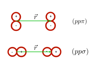
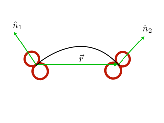
Figure 1: Left: The two independent, $r$-dependent integrals $(pp\sigma)$ and $(pp\pi)$ for $p$-orbitals. For flat graphene, only the first one is relevant. Right: For graphene with curvature, $p$-orbitals are no longer parallel.

The usual assumption when dealing with non-planar strains is that off-plane atomic displacements $h(\vec{r})$ enter the hamiltonian only through the combination ${u}_{ij}=(\partial_{i}\xi_{j}+\partial_{j}\xi_{i}+\partial_{i}h\partial_{j}h)/2$. The rationale is that the distance between two nearby points is given by $ds^{2}=(\delta_{ij}+2u_{ij})dx^{i}dx^{j}$ where $dx^{i}$ is the difference between the equilibrium coordinates of the two points. However, this is be justified if the matrix elements between orbitals belonging to different atoms depend only on the distance, which is valid for $s$-orbitals, but integrals involving $p_{z}$-orbitals are non-isotropic. To be concrete, whereas integrals involving two $s$-orbitals are parametrized by a single function of the distance, usually denoted $(ss\sigma)$, two independent functions are required in the case of $p$-orbitals. These are denoted $(pp\sigma)$ and $(pp\pi)$, see Fig. 1. For flat graphene, only $(pp\pi)=-t_{1}$ is relevant, and in this respect $p_{z}$-orbitals behave just like $s$-orbitals.

However, in presence of curvature the two $p_{z}$-orbitals are no longer parallel Huertas-Hernando et al. (2006). In terms of $(pp\sigma)\equiv f_{\sigma}(r)$ and $(pp\pi)\equiv f_{\pi}(r)$, one can use linearity to show that the matrix element is then given by

$$\langle\Phi_{1}|H|\Phi_{2}\rangle=(\hat{n}_{1}\cdot\hat{r})(\hat{n}_{2}\cdot\hat{r})f_{\sigma}(r)+[\hat{n}_{1}-(\hat{n}_{1}\cdot\hat{r})\hat{r}]\cdot[\hat{n}_{2}-(\hat{n}_{2}\cdot\hat{r})\hat{r}]f_{\pi}(r),$$ (14)

where $\hat{n}_{i}$ are unit vectors parallel to the $p$-orbitals, which may be assumed to be perpendicular to the surface. This has a rather involved dependence, not only on $r$, but also on the angles. Thus, the assumption that the hamiltonian depends on $h$ only through Eq. (1) is not valid in general for curved graphene.

On the other hand, in order to have curvature we need non-vanishing second derivatives of $h$. This means that couplings involving only first derivatives of $h$ are independent of the $(pp\pi)$ integrals and, as a result, their dependence on off-plane strains is only through $u_{ij}$. As only $H_{6}$ and $\tilde{H}_{6}$ involve second derivatives of $h$, we see that, with the usual approximations implicit in TB, $\tilde{a}_{i}\!=\!0$ for $i=1,\ldots,5$. Expanding eq. (14) to the appropriate order it is easy to see that the first non-vanishing contribution is proportional to second derivatives of the strain and, as a consequence, the coefficient $\tilde{a}_{6}$ vanishes. This is true in the reference system of the perfect lattice (crystal frame). Frame effects will be discussed in the next subsection.

IV.2 Lab frame effects

Lab frame effects are the result of the change from crystal to laboratory coordinates, as was discussed in detail in ref. de Juan et al., 2013. As a consequence, new terms independent of the TB couplings appear in the Hamiltonian. Crystal coordinates $\{x\}$ are just the atomic equilibrium positions. If we define the laboratory coordinates $\{y_{i}\}$ as the horizontal projections of the out-of-equilibrium positions, $y_{i}=x_{i}+\xi_{i}(x)$, then a change of variables in the continuum Hamiltonian gives the result de Juan et al. (2013):

$$\hat{H}_{Lab}=\hat{H}_{TB}+\hat{H}_{Geom},$$ (15)

where $\hat{H}_{TB}$ is the hamiltonian in the crystal frame and

$$\hat{H}_{Geom}=v_{F}\!\int d^{2}x\,\tilde{u}_{kl}(\psi^{\dagger}\sigma_{k}\overleftrightarrow{\partial_{l}}\psi)$$ (16)

with $\tilde{u}_{ij}=\frac{1}{2}(\partial_{i}\xi_{j}+\partial_{j}\xi_{i})$. Comparing with Table 2, we see that $\hat{H}_{Geom}$ is proportional to $\hat{H}_{5}$ with $u_{ij}$ replaced by $\tilde{u}_{ij}$. Thus both $a_{5}$ and $\tilde{a}_{5}$ are corrected to compensate for the absence of the non-linear piece in $\tilde{u}_{ij}$:

$$\delta a_{5}=-\delta\tilde{a}_{5}=v_{F}.$$ (17)

We have summarized our knowledge of the laboratory couplings in Table 6.

$a_{1}$	$\;\;\;\frac{3\sqrt{3}}{2}t_{2}^{\prime}a+\frac{3}{2}V^{\prime}a\;\;\;$	$\tilde{a}_{1}$	$0$
$a_{2}$	$\frac{\beta}{2a}v_{F}$	$\tilde{a}_{3}$	$0$
$a_{3}$	​​​$-\frac{9\sqrt{3}}{4}t^{\prime}_{2}a^{2}$	$\tilde{a}_{2}$	$0$
$a_{4}$	$\frac{\beta}{4}v_{F}$	$\tilde{a}_{4}$	$0$
$a_{5}$	$(\frac{\beta}{2}+1)v_{F}$	$\tilde{a}_{5}$	$\;\;-v_{F}\;\;$
$a_{6}$	$\frac{3}{8}V^{\prime}a^{2}$	$\tilde{a}_{6}$	0

Table 6: Lab frame couplings for the effective hamiltonian.

IV.3 Pseudo–Zeeman term

As discussed in Sec. III, $H_{6}$ is a new term which describes the direct coupling of the $z$-component of pseudospin to the pseudomagnetic field $B$. This term plays the role of a mass in the Dirac fermion effective theory and opens a gap in the spectrum. This mechanism is different from the various proposals of gap opening by strain in the literature, such as the the gap associated to the the Landau levels Low and Guinea (2010); Guinea et al. (2010b); Low et al. (2011); Ferone et al. (2011), superlattices Park et al. (2008); Snyman (2009); Guinea and Low (2010); Naumov and Bratkovsky (2011), or by merging of the Fermi points by strain Pereira et al. (2009); Cocco et al. (2010). It is analogous to the one obtained by an on-site potential that is opposite in the two sublattices (note that the required strain breaks inversion symmetry as well), but offers the additional advantage of being tunable by the externally induced strain. This type of diagonal terms coming from strain have been recently discussed in ref. Barraza-Lopez et al., 2013 in an approach which uses directly the atomic displacements without reference to continuous elasticity theory.

The order of magnitude of this gap may be estimated with the case of a ripple of moderate strain with height $h=5\mathrm{\AA}$ and width $l=25\mathrm{\AA}$, which gives a pseudomagnetic field of

$$B\approx\frac{1}{l}\frac{h^{2}}{l^{2}}=0.0016\mathrm{\AA}^{-1},$$ (18)

and an energy gap of the order of

$$E_{{\mathcal{Z}eeman}}=3/8V^{\prime}a^{2}B\sim 7meV,$$ (19)

were we have taken the value $V^{\prime}=6eV/\mathrm{\AA}$ from ref. Ferone et al., 2011. The presence of this new term has several interesting implications. As it is known, the orbital coupling of elastic pseudomagnetic fields comes with opposite signs in the two Fermi points so that the combined effect of real and pseudomagnetic fields gives rise to valley separation effects Guinea et al. (2008b, 2010a); Jiang et al. (2013); Vaezi et al. (2013), and the same is expected for the Zeeman coupling. Indeed, in the presence of high magnetic fields, the zero-th Landau Level will be split by a controlled pseudo-Zeeman coupling and induce valley polarization. In addition to providing a measurement of the coefficient $a_{6}$, this may help to understand the origin of the observed interaction-induced splittingsGoerbig (2011); Kharitonov (2012); Young et al. (2012) –which can be of similar magnitude at moderate field Barlas et al. (2012)– by studying the dependence of the gap with the pseudo–field, and the competition with the real Zeeman coupling. As a related effect, the in-plane distortion that generates this splitting may be induced spontaneously via a Peierls instability, by the same mechanism as the out-of-plane distortion studied in ref. Fuchs and Lederer, 2007.

V Summary and discussion

In this work we have used a symmetry approach to construct all possible terms affecting the low energy properties of graphene in the presence of non-uniform lattice deformations. We have limited our analysis to linear elasticity theory and assumed that the two Fermi points do not mix, which is a sensible assumption for reasonably smooth strains.

As we are primarily interested in the effects of non-uniform strain, we have set up a derivative expansion of the effective hamiltonian and used group theory techniques to obtain the number of independent couplings at each derivative order. This procedure guarantees that no relevant interactions are left out. Then we have constructed the interactions in a completely model independent way.

After a careful analysis of the physical effects of the interactions and the properties of the derivative expansion, we have argued that the first order effective hamiltonian in Eq. (2) is “phenomenologically complete”, in the sense that any additional terms that we might construct would not give rise to qualitatively different physical phenomena, they would just provide higher order corrections. Under most experimental circumstances these corrections would be strongly suppressed and very hard to measure.

In order to get an estimate of the values of the twelve coupling constants parametrizing the effective hamiltonian, we have considered a generalized tight binding model. This model incorporates, besides first and second nearest neighbor hoppings, the contribution of a nearest neighbor potential to the on-site energy of an electron in a $p_{z}$-orbital. This contribution, which is not often included in the tight binding hamiltonian, is necessary in order to account for the new gap-opening pseudo-Zeeman term coupling of pseudospin and pseudomagnetic field. This, and the fact that the pseudo-Zeeman term appears at first derivative order, while most tight binding computations are carried out for uniform strains, are the probable reasons why this term had gone unnoticed. This highlights the importance of the symmetry approach as a way to get all the allowed interactions in a model independent way.

In this paper we have neglected electron spin, but our analysis could be easily extended to accommodate it along the lines of Ref. Ochoa et al., 2012. Anharmonic effects are supposed to play an important role in the mechanical properties of graphene Zakharchenko et al. (2010); Castro et al. (2010); de Andres et al. (2012) although this assertion is yet to be confirmed by the experiments Lu and Huang (2009). On the other hand, their effects on the pseudomagnetic field has been considered recently in Ref. Ramezani Masir et al., 2013 using a tight binding model. The techniques presented in this paper can be easily extended to compute, in a model independent way, all the allowed terms in an expansion in powers of the strain. Another possible extension is to include the effects of optical strains or frozen optical modes, which may affect the electronic properties of graphene on a substrate. Their effects on the pseudomagnetic fields at leading derivative order were considered in Ref. Mañes, 2007 and have been recently incorporated in an effective hamiltonian Linnik (2012). Our methods could be used to explore their contributions at higer derivative orders.

Appendix A The symmetry construction

In this Appendix we give a brief account of the group theory techniques used to construct the effective hamiltonian. As mentioned in Section II, as long as we neglect interactions between the two inequivalent Dirac points we can restrict ourselves to the symmetries that leave $K_{1}$ invariant, i.e., to the little group of $K_{1}$. The little point group $C_{3v}$ consists of six elements: the identity operation $E$, two $\pm 2\pi/3$ rotations $C_{3}^{\pm}$ around the $OZ$ axis and three reflections $\sigma_{vi}$ by vertical planes. Transformation properties under $C_{3v}$ are classified by three irreducible representations (IRs): $A_{1}$ and $A_{2}$ are one-dimensional, whereas $E$ is two-dimensional. Their character tables together with their products Bradley and Cracknell (2010) are given in Table 7.

$$\begin{array}[]{c c}\begin{array}[]{|c||c|c|c|}\hline\cr C_{3v}&E&C_{3}^{\pm}&\sigma_{vi}\\ \hline\cr\hline\cr A_{1}&1&1&1\\ \hline\cr A_{2}&1&1&-1\\ \hline\cr E&2&-1&0\\ \hline\cr\end{array}&\;\;\;\;\;\;\begin{array}[]{|c||c|c|c|}\hline\cr C_{3v}&A_{1}&A_{2}&E\\ \hline\cr\hline\cr A_{1}&A_{1}&A_{2}&E\\ \hline\cr A_{2}&A_{2}&A_{1}&E\\ \hline\cr E&E&E&A_{1}+A_{2}+E\\ \hline\cr\end{array}\end{array}$$

Table 7: Left: characters of the three irreducible representations of $C_{3v}$. Right: decomposition of all possible product of two irreducible representations.

Graphene is also invariant under time-reversal $\theta$, which takes the Dirac point $K_{1}$ into $K_{2}$, $\theta K_{1}\equiv K_{2}$. The same is accomplished by $C_{2}$, which is $180$ degree rotation around the $OZ$ axis and belongs to the point group $C_{6v}$. Thus, the combined antiunitary operation $\theta C_{2}$ leaves $K_{1}$ invariant and imposes additional restrictions on the allowed interactions.

Table 8 gives the transformation properties of all the ingredients used in the construction of the effective hamiltonian for strained graphene. For the sake of completeness, we have included the antisymmetric part of $\partial_{i}\xi_{j}$, which represents a local rotation. Note that the transformation properties of the Pauli matrices follow from those of the electronic states. More concretely, the two components of the electron field $(\psi_{1},\psi_{2})$ transform according to the irreducible representation $E$. Then the set of four $2\times 2$ hermitian matrices belong to the reducible representation $E\times E$, which decomposes according to

$$E\times E=A_{1}(\openone)+A_{2}(\sigma_{z})+E(\sigma_{x},\sigma_{y}).$$ (20)

Magnitudes	IR of $C_{3v\;}$	$\ \theta C_{2}\;$
$\openone$, $u_{xx}+u_{yy}$	$A_{1}$	$+$
$\omega$	$A_{2}$	$+$
$\sigma_{z}$	$A_{2}$	$-$
$(u_{xx}-u_{yy},-2u_{xy})$, $(k_{x},k_{y})$, $(\sigma_{x},\sigma_{y})$	$E$	$+$
$(\partial_{x},\partial_{y})$	$E$	$-$

Table 8: Transformation properties under the little group of $K_{1}$. The antisymmetric part of $\partial_{i}\xi_{j}$ is given by the local rotation $\omega=\partial_{x}\xi_{y}-\partial_{y}\xi_{x}$.

Group theory can now be used to obtain the number of independent terms in the effective hamiltonian at order $(n_{q},n_{k})$. The basic formula is Bradley and Cracknell (2010)

$$n=\frac{1}{N}\sum_{g}\chi_{T}(g),$$ (21)

where $n$ is the number independent invariants, $N$ is the number of elements $g$ in the group and $\chi_{T}(g)$ is the character of $g$ in the representation $T$ associated to the interaction term. The character $\chi_{T}(g)$ is generally obtained as the product of the characters of the representations corresponding to the different components of the interaction term. As an example, assume that we want to know the number of independent terms of order $(n_{q},n_{k})=(0,1)$ containing the matrices $\sigma_{x},\sigma_{y}$. This involves the quantities $u_{ij}$, $k_{i}$ and $\sigma_{i}$, which according to Table 8 belong to the representations $A_{1}+E$, $E$ and $E$ respectively. Thus

$$\chi_{T}=(\chi_{A_{1}}+\chi_{E})\times\chi_{E}\times\chi_{E},$$ (22)

which implies

$$\chi_{T}(E)=12\;\;\;,\;\;\;\chi_{T}(C_{3}^{\pm})=\chi_{T}(\sigma_{vi})=0.$$ (23)

Then Eq. (21) gives $n\!=\!2$.

Note that according to Table 8, both $\sigma_{z}$ and the derivatives $\partial_{i}$ acting on the strain are odd under $\theta C_{2}$. Thus, terms proportional to the matrices $\{\openone,\sigma_{x},\sigma_{y}\}$ must contain an even number of derivatives of the strain, whereas this number must be odd for terms proportional to $\sigma_{z}$. The results of using this method for $n_{k}+n_{q}\leq 2$ are summarized in Table 1 of Sect. II. The number of invariants involving $\omega$ instead of $u_{ij}$ is given in Table 4.

Invariant interactions, which by definition transform like $(A_{1},+)$, can be obtained by using the following composition rules for the IRs of $C_{3v}$:

$$A_{1}(a)\times E(b_{1},b_{2}) = E(ab_{1},ab_{2})$$

$$A_{2}(a)\times E(b_{1},b_{2}) = E(ab_{2},-ab_{1})$$

$$E(a_{1},a_{2})\times E(b_{1},b_{2}) = A_{1}(a_{1}b_{1}+a_{2}b_{2})+A_{2}(a_{1}b_{2}-a_{2}b_{1})+E(a_{1}b_{1}-a_{2}b_{2},-a_{1}b_{2}-a_{2}b_{1}).$$ (24)

For one-dimensional IRs, we have $A_{1}(a)\times A_{1}(b)=A_{1}(ab)$, $A_{2}(a)\times A_{2}(b)=A_{1}(ab)$ and $A_{1}(a)\times A_{2}(b)=A_{2}(ab)$. Several examples of the use of these realtions are given at the end of this Appendix.

Once an interaction term has been constructed around $K_{1}$, we can use the time reversal operation $\theta$ to construct the corresponding interaction around the other Dirac point $K_{2}$. Time reversal acts by complex conjugation, and its action on the different objects is given in the l.h.s. of Table 9 for the the usual $(A_{1},B_{1},A_{2},B_{2})$ sublattice convention.

As an example, the Dirac hamiltonian $k_{x}\sigma_{x}+k_{y}\sigma_{y}$ at $K_{2}$ is given by

$$\theta:k_{x}\sigma_{x}+k_{y}\sigma_{y}\rightarrow-k_{x}\sigma_{x}+k_{y}\sigma_{y}.$$ (25)

In order to compare interaction hamiltonians at the two Dirac points, we have to take into account that even $H_{0}$ differs by the sign of $k_{x}$. This fact, which makes a direct comparison awkward, can be avoided by a change of basis at $K_{2}$. Conjugation of the Pauli matrices by $\sigma_{y}$ yields

$$\sigma_{y}(\openone,\sigma_{x},\sigma_{y},\sigma_{z})\sigma_{y}=(\openone,-\sigma_{x},\sigma_{y},-\sigma_{z})$$ (26)

and now $H_{0}$ takes the same form at the two Dirac points

$$\sigma_{y}(-k_{x}\sigma_{x}+k_{y}\sigma_{y})\sigma_{y}=k_{x}\sigma_{x}+k_{y}\sigma_{y}.$$ (27)

Conjugation by $\sigma_{y}$ changes the sublattice convention to $(A_{1},B_{1},B_{2},A_{2})$. This is summarized in the r.h.s. of Table 9, which can be used to obtain the hamiltonian at $K_{2}$ after conjugation by $\sigma_{y}$. Note that now all three Pauli matrices are odd under time reversal.

$$\begin{array}[]{c c}\begin{array}[]{|c || c |}\hline\cr\mathrm{Magnitudes}&\ \theta\\ \hline\cr\hline\cr u_{ij},\omega,\partial_{i},\openone,\sigma_{x},\sigma_{z}&+\\ k_{i},\sigma_{y}&-\\ \hline\cr\end{array}&\;\;\;\;\;\;\;\;\;\;\;\;\begin{array}[]{|c || c |}\hline\cr\mathrm{Magnitudes}&\ \theta\\ \hline\cr\hline\cr u_{ij},\omega,\partial_{i},\openone&+\\ k_{i},\vec{\sigma}&-\\ \hline\cr\end{array}\end{array}$$

Table 9: Transformation properties under time reversal with the $(A_{1},B_{1},A_{2},B_{2})$ convention (left), and with the $(A_{1},B_{1},B_{2},A_{2})$ convention used in this paper (right).

We finish this Appendix with a few examples:

• The fourth line in Table 8 together with the third line in Eq. (A) show that the Dirac hamiltonian $H_{0}=k_{x}\sigma_{x}+k_{y}\sigma_{y}$ is invariant. Concretely,

  $$E(k_{x},k_{y})\times E(\sigma_{x},\sigma_{y}) = A_{1}(k_{x}\sigma_{x}+k_{y}\sigma_{y})+\ldots$$ (28)

• The fourth line in Table 8 together the third line in Eq. (A) imply that $H_{2}=(u_{xx}-u_{yy})\sigma_{x}-2u_{xy}\sigma_{y}$ is invariant. Using Table 9 to obtain $H_{2}$ at $K_{2}$ gives

  $$(u_{xx}-u_{yy})\sigma_{x}-2u_{xy}\sigma_{y}\rightarrow-(u_{xx}-u_{yy})\sigma_{x}+2u_{xy}\sigma_{y},$$ (29)

  showing that pseudogauge fields have opposite signs at the two Dirac points.

• The fourth and fifth lines in Table 8 together with the third line in Eq. (A) show that $\partial_{y}(u_{xx}-u_{yy})+2\partial_{x}u_{xy}$ transforms according to $(A_{2},-)$. Concretely,

  $$E(\partial_{x},\partial_{y})\times E(u_{xx}-u_{yy},-2u_{xy}) = A_{2}[\partial_{y}(u_{xx}-u_{yy})+2\partial_{x}u_{xy}]+\ldots$$ (30)

  Then $A_{2}\times A_{2}=A_{1}$ and the third line in Table 8 imply that $H_{6}=\big{[}\partial_{y}(u_{xx}-u_{yy})+2\partial_{x}u_{xy}\big{]}\mathbf{\sigma}_{z}$ is invariant (Zeeman coupling for pseudospin).

Appendix B Generalized tight binding model

In this Appendix we fix our conventions and give details on the tight binding model used to compute the coupling constants. We choose a coordinate system such that the vectors $\vec{v}_{n}$ to the three NN are given by

$$\vec{v}_{1}=a(0,1)\;\;\;,\;\;\;\vec{v}_{2}=-\frac{a}{2}(\sqrt{3},1)\;\;\;,\;\;\;\vec{v}_{3}=\frac{a}{2}(\sqrt{3},-1)$$ (31)

where $a$ is the distance between NN. The vectors to the six NNN are given by

$$\vec{w}_{1}=-\vec{w}_{4}=-a(\sqrt{3},0)\;\;\;,\;\;\;\vec{w}_{2}=-\vec{w}_{5}=-\frac{a}{2}(\sqrt{3},3)\;\;\;,\;\;\;\vec{w}_{3}=-\vec{w}_{6}=\frac{a}{2}(\sqrt{3},-3)$$ (32)

and the Fermi points are located at $\vec{K}_{1}=-\vec{K}_{2}=(\frac{4\pi}{3\sqrt{3}a},0)$

A general displacement

$$\vec{\xi}(\vec{r})=\sum_{\vec{q}}\vec{\xi}(\vec{q}\,)e^{i\vec{q}\cdot\vec{r}}\;\;\mathrm{with}\;\;\;\vec{\xi}(-\vec{q}\,)=\vec{\xi}(\vec{q}\,)^{*}$$ (33)

induces a change in the vectors that go from an atom at position $\vec{t}+\vec{r}_{1}$ to its nearest neighbors

$$\delta\vec{v}_{n}=\sum_{\vec{q}}\vec{\xi}(\vec{q}\,)e^{i\vec{q}\cdot(\vec{t}+\vec{r}_{1})}\left[e^{i\vec{q}\cdot\vec{v}_{n}}-1\right],$$ (34)

with a similar expression for $\delta\vec{w}_{n}$. To linear order in $\vec{\xi}_{i}$, this induces a change in the NN hopping integral

$$\delta t_{1}(\vec{t})=\vec{\nabla}t_{1}\!\cdot\delta\vec{v}_{n}=t_{1}^{\prime}\,\sum_{\vec{q}}(\vec{\xi}(\vec{q}\,)\cdot\hat{v}_{n})e^{i\vec{q}\cdot(\vec{t}+\vec{r}_{1})}\left[e^{i\vec{q}\cdot\vec{v}_{n}}-1\right]$$ (35)

with analogous expressions for $\delta t_{2}$ and $\delta V$. Then, substituting (35) into

$$\delta H_{12}(\vec{q},\vec{k}\,)=\langle\Phi_{1}(\vec{k}+\frac{1}{2}\vec{q}\,)|\delta H|\Phi_{2}(\vec{k}-\frac{1}{2}\vec{q}\,)\rangle=-\frac{1}{N}\sum_{\vec{t},n}\delta t_{1}(\vec{t})e^{-i\vec{q}\cdot(\vec{t}+\vec{r}_{1})}e^{i(\vec{k}-\frac{\vec{q}}{2})\cdot\vec{v}_{n}}$$ (36)

and doing the sum over the Bravais lattice vectors $\{\vec{t}\}$ yields

$$\delta H_{12}(\vec{q},\vec{k}\,)=-2it^{\prime}_{1}\sum_{n=1}^{3}\vec{\xi}(\vec{q}\,)\cdot\hat{v}_{n}e^{i\vec{v}_{n}\cdot(\vec{K}_{1}+\vec{k})}\sin\bigl{(}\frac{\vec{q}\cdot\vec{v}_{n}}{2}\bigr{)}.$$ (37)

The same method is used to obtain the other matrix elements.

References

- Meyer et al. (2007) J. C. Meyer, A. K. Geim, M. I. Katsnelson, K. S. Novoselov, T. J. Booth, and S. Roth, Nature 446, 60 (2007).
- Lee et al. (2009) C. Lee, X. Wei, J. W. Kysar, and J. Hone, Science 321, 5887 (2009).
- Kim et al. (2009) K. S. Kim et al., Nature 457, 706 (2009).
- Tomori et al. (2011) H. Tomori, A. Kanda, H. Goto, Y. Ootuka, K. Tsukagoshi, S. Moriyama, E. Watanabe, and D. Tsuya, Applied Physics Express 4, 075102 (2011).
- Suzuura and Ando (2002) H. Suzuura and T. Ando, Phys. Rev. B 65, 235412 (2002).
- Guinea et al. (2008a) F. Guinea, B. Horovitz, and P. L. Doussal, Phys. Rev. B 77, 205421 (2008a).
- Vozmediano et al. (2010) M. A. H. Vozmediano, M. I. Katsnelson, and F. Guinea, Phys. Reports 496 (2010).
- Decker et al. (2011) R. Decker, Y. Wang, V. W. Brar, W. Regan, H. Tsai, Q. Wu, W. Gannett, A. Zettl, and M. F. Crommie, NanoLetters 11, 2291 (2011).
- Gomes et al. (2012) K. K. Gomes, W. Mar, W. Ko, F. Guinea, and H. C. Manoharan, Nature 483, 306 (2012).
- de Juan et al. (2007) F. de Juan, A. Cortijo, and M. A. H. Vozmediano, Phys. Rev. B 76, 165409 (2007).
- de Juan et al. (2012) F. de Juan, M. Sturla, and M. A. H. Vozmediano, Phys. Rev. Lett. 108, 227205 (2012).
- Kitt et al. (2012) A. L. Kitt, V. M. Pereira, A. K. Swan, and B. B. Goldberg, Phys. Rev. B 85, 115432 (2012).
- Kitt et al. (2013) A. L. Kitt, V. M. Pereira, A. K. Swan, and B. B. Goldberg, Phys. Rev. B 87, 159909(E) (2013).
- de Juan et al. (2013) F. de Juan, J. L. Mañes, and M. A. H. Vozmediano, Phys. Rev. B 87, 165131 (2013).
- Ramond (1997) P. Ramond, Field theory: A modern primer (Perseus Books, 1997).
- Landau (1957) L. D. Landau, Soviet Physics JETP 3, 920 (1957).
- Slonczewski and Weiss (1958) J. C. Slonczewski and P. R. Weiss, Phys. Rev. 109, 272 (1958).
- Mañes (2007) J. L. Mañes, Phys. Rev. B 76, 045430 (2007).
- Winkler and Zulicke (2010) R. Winkler and U. Zulicke, Phys. Rev. B 82, 245313 (2010).
- Ferone et al. (2011) R. Ferone, J. R. Walbank, V. Zolyomi, and V. I. Falḱo, Sol. St. Commun. 151, 1071 (2011).
- Linnik (2012) T. L. Linnik, J. Phys.: Condens. Matter 24, 205302 (2012).
- Cabra et al. (2013) D. C. Cabra, N. E. Grandi, G. A. Silva, and M. B. Sturla, Phys. Rev. B 88, 045126 (2013).
- Basko (2008) D. M. Basko, Phys.Rev. B 78, 125418 (2008).
- Ochoa et al. (2012) H. Ochoa, A. H. C. Neto, V. I. Falḱo, and F. Guinea, Phys. Rev. B 86, 245411 (2012).
- Guinea et al. (2010a) F. Guinea, M. I. Katsnelson, and A. G. Geim, Nature Physics 6, 30 (2010a).
- Castro Neto et al. (2009) A. H. Castro Neto, F. Guinea, N. M. R. Peres, K. S. Novoselov, and A. K. Geim, Rev. Mod. Phys. 81, 109 (2009).
- Mañes et al. (2007) J. L. Mañes, F. Guinea, and M. Vozmediano, Phys. Rev. B 75, 155424 (2007).
- Bradley and Cracknell (2010) C. J. Bradley and A. P. Cracknell, The Mathematical Theory of Symmetry in Solids (Oxford University Press, 2010).
- Low et al. (2011) T. Low, F. Guinea, and M. I. Katsnelson, Phys. Rev B 83, 195436 (2011).
- Kobayashi et al. (2007) A. Kobayashi, S. Katayama, Y. Suzumura, and H. Fukuyama, J. Phys. Soc. Jpn. 76, 034711 (2007).
- Goerbig et al. (2008) M. O. Goerbig, J. Fuchs, G. Montambaux, and F. Piechon, Phys. Rev. B 78, 045415 (2008).
- Wunsch et al. (2008) B. Wunsch, F. Guinea, and F. Sols, New J. Phys. 10, 103027 (2008).
- Montambaux et al. (2009) G. Montambaux, F. Piechon, J. Fuchs, and M. O. Goerbig, Phys. Rev. B 80, 153412 (2009).
- Choi et al. (2010) S. Choi, S. Jhi, and Y. Son, Phys. Rev. B 81, 081407(R) (2010).
- Guinea et al. (2008b) F. Guinea, M. I. Katsnelson, and M. A. H. Vozmediano, Phys. Rev. B 77, 075422 (2008b).
- Brey and Palacios (2008) L. Brey and J. J. Palacios, Phys. Rev. B 77, 041403(R) (2008).
- Zhang et al. (2009) Y. Zhang, V. W. Brar, C. Girit, A. Zettl, and M. F. Crommie, Nature Physics 5, 722 (2009).
- Gazit (2009) D. Gazit, Phys. Rev. B 80, 161406(R) (2009).
- Gibertini et al. (2012) M. Gibertini, A. Tomadin, F. Guinea, M. I. Katsnelson, and M. Polini, Phys. Rev. B 85, 201405(R) (2012).
- Pellegrino et al. (2011) F. M. D. Pellegrino, G. G. N. Angilella, and R. Pucci, Phys. Rev. B 84, 195404 (2011).
- Zhang et al. (2013) Y. Zhang, C. Luo, W. Lia, and C. Pan, Nanoscale 5, 2616 (2013).
- Konschuh et al. (2010) S. Konschuh, M. Gmitra, and J. Fabian, Phys. Rev. B 82, 245412 (2010).
- Sloan et al. (2013) J. V. Sloan, A. A. P. Sanjuan, Z. Wang, C. Horvath, and S. Barraza-Lopez, Phys. Rev. B 87, 155436 (2013).
- Barraza-Lopez et al. (2013) S. Barraza-Lopez, A. A. Pacheco, Z. Wang, and M. Vanevic, Solid State Communications 166, 70 (2013).
- Huertas-Hernando et al. (2006) D. Huertas-Hernando, F. Guinea, and A. Brataas, Phys. Rev. B. 74, 155426 (2006).
- Low and Guinea (2010) T. Low and F. Guinea, Nano Lett. 10, 3551 (2010).
- Guinea et al. (2010b) F. Guinea, A. G. Geim, M. I. Katsnelson, and K. S. Novoselov, Phys. Rev. B 81, 035408 (2010b).
- Park et al. (2008) C. Park, L. Yang, Y. Son, M. L. Cohen, and S. G. Louie, Nat. Phys. 4, 213 (2008).
- Snyman (2009) I. Snyman, Phys. Rev B 80, 054303 (2009).
- Guinea and Low (2010) F. Guinea and T. Low, Phil. Trans. R. Soc. A 368, 05391 (2010).
- Naumov and Bratkovsky (2011) I. I. Naumov and A. M. Bratkovsky, Phys. Rev B 84, 245444 (2011).
- Pereira et al. (2009) V. M. Pereira, A. H. Castro Neto, and N. M. R. Peres, Phys. Rev. B 80, 045401 (2009).
- Cocco et al. (2010) G. Cocco, E. Cadelano, and L. Colombo, Phys. Rev B 81, 241412(R) (2010).
- Jiang et al. (2013) Y. Jiang, T. Low, K. Chang, M. I. Katsnelson, and F. Guinea, Phys. Rev. Lett. 110, 046601 (2013).
- Vaezi et al. (2013) A. Vaezi, N. Abedpour, R. Asgari, A. Cortijo, and M. A. H. Vozmediano, Phys. Rev. B 88, 125406 (2013).
- Goerbig (2011) M. O. Goerbig, C. R. Physique 12, 369 (2011).
- Kharitonov (2012) M. Kharitonov, Phys. Rev. B 85, 155439 (2012).
- Young et al. (2012) A. F. Young et al., Nat. Phys. 8, 550 (2012).
- Barlas et al. (2012) Y. Barlas, K. Yang, and A. H. MacDonald, Nanotechnology 23, 052001 (2012).
- Fuchs and Lederer (2007) J.-N. Fuchs and P. Lederer, Phys. Rev. Lett. 98, 016803 (2007).
- Zakharchenko et al. (2010) K. V. Zakharchenko, R. Roldan, A. Fasolino, and M. I. Katsnelson, Phys. Rev. B 82, 125435 (2010).
- Castro et al. (2010) E. V. Castro, H. Ochoa, M. I. Katsnelson, R. V. Gorbachev, D. C. Elias, K. S. Novoselov, A. K. Geim, and F. Guinea, Phys. Rev. Lett. 105, 266601 (2010).
- de Andres et al. (2012) P. L. de Andres, F. Guinea, and M. I. Katsnelson, Phys. Rev. B 86, 144103 (2012).
- Lu and Huang (2009) Q. Lu and R. Huang, Int. Journal of Applied Mechanics 1, 443 (2009).
- Ramezani Masir et al. (2013) M. Ramezani Masir, D. Moldovan, and F. M. Peeters, Solid State Commun. 175-176, 76 (2013).