Model-free measure of coupling from embedding principle

Abstract

A model-free measure of coupling between dynamical variables is built from time series embedding principle. The approach described does not require a mathematical form for the dynamics to be assumed. The approach also does not require density estimation which is an intractable problem in high dimensions. The measure has strict asymptotic bounds and is robust to noise. The proposed approach is used to demonstrate coupling between complex time series from the finance world.

Probing for coupling between dynamical variables is a problem of fundamental interest in a variety of disciplines. In real world settings the underlying model is often unknown and we only have time series measurements. An information-theoretic approach seeks to assess coupling between two time series measurements by ascertaining if additional information about the future state of a variable can be gained by including the second variable in a discriminative model. This measure which is popularly termed transfer entropy finds the difference between conditional entropy of future states between models that contain and do not contain the second variableschreiber2000measuring . The notion of determining coupling via a predictability approach also forms the basis of Granger causality which addresses the same question by assessing the predictability of one of the variables using linear autoregressive models in which the second variable is present or absentgranger1969investigating . The Granger approach has been generalized to the nonlinear case by using a nonlinearly transformed feature spacemarinazzo2008kernel . Transfer entropy and Granger causality were shown to be equivalent for Gaussian variablesbarnett2009granger . While determining coupling via the predictability mechanism notionally appears to be true, the idea has never been mathematically established, both in transfer entropy and Granger causality. Moreover, these measures do not have any asymptotic limitkaiser2002information . A zero transfer entropy in one direction must be obtained in order to conclude directionalitykaiser2002information . However, the measure depends on accurate evaluation of conditional densities which is often obtained by expressing those in terms of joint probabilities. The density evaluation suffers from bias and in practice one obtains a nonzero value of transfer entropy even for cases where it is theoretically supposed to be zerokaiser2002information ; Staniek . Staniek et alStaniek proposed symbolic quantization using ordinal patterns for density estimation. The directionality of coupling for example in this case was ascertained by comparing two values for transfer entropy where the driving variables are switched. The absolute value of these entropies however cannot be compared with another case. Transfer entropy calculation returns a nonzero value due to statistical bias in density estimation both for uncoupled and fully synchronized variablesStaniek . This makes it difficult to distinguish between these two cases. In both the approaches above, a very important parameter is the memory or Markov order of the underlying dynamical process. This parameter is chosen in an ad hoc manner. Some processes can have long memory which warrants that even a model-free measure of transfer entropy must ascertain these high dimensional densities. This is especially true for deterministic complex signals such as those found in a chaotic system.

The above highlighted issues are addressed in this paper by presenting a unified framework for coupling detection. Following are the salient features of the proposed framework:

1. A model-free measure of Markov order is first used in determining the memory of the dynamical system.

2. The measure of coupling is built from state space reconstruction based on first principles. A necessary condition for coupling is first established. A measure is then built to assess this necessary condition.

3. This measure is convergent to an asymptotic absolute limit both for uncoupled and fully coupled cases. The lower bound is zero for completely uncoupled variables and the upper bound is one for fully coupled variables. The proposed approach is the best way to avoid false positives owing to a strict lower bound which is not affected by the amount of noise in the signal. Detection of true positives is also robust to the presence of a large amount of noise.

4. The approach is model-free and therefore is not limited by the assumptions of a parametric model.

5. The approach can distinguish between uncoupled and fully synchronized systems. Fully synchronized systems can be detected with the measure taking a value of one.

The outline of this paper is as follows: Section I establishes the necessary condition for two variables to be coupled from attractor reconstruction based first principles. Section II elaborates a statistical measure to assess this necessary condition. This completes the foundation for this work. Section III explains an approach to determine the Markov order of a time series. Section IV discusses the choice of appropriate time series embedding for the methodology described in this paper. Section V introduces the procedure by probing for coupling between $x$ and $y$ variables of Rossler system. Robustness of statistics to noise is also demonstrated. Section VI conjectures that the proposed approach can also be used to ascertain the directionality of coupling and this is demonstrated with the help of asymmetrically coupled Lorenz system. The effectiveness of the approach to distinguish between uncoupled and fully synchronized systems is also discussed. In Section VII, the application of this method is demonstrated on an example from the finance world. It is shown that the currency exchange rate Canadian Dollar-Japanese Yen and oil prices are strongly coupled. Section VIII concludes the findings of this paper.

I Necessary condition for coupling

Consider a dynamical system

$$\dot{\mathbf{x}}=f\left(\mathbf{x}\right)$$ (1)

where $\mathbf{x}\in\mathbb{R}^{n}$ is the state vector of the system. Let $x_{1},\leavevmode\nobreak\ x_{2},...,x_{n}$ be the state variables. Let $\mathbb{M}$ be the manifold on which the states of the system asymptotes as it evolves over time. This manifold is termed as the attractor of the system. For an attractor manifold $\mathbb{M}$ with $\mathbf{x}(t)$ as the state of the system at time $t$ and flow $f:\mathbb{M}\to\mathbb{M}$, the manifold defined by the $F(h,f,\tau_{1},...,\tau_{m}):\mathbb{M}\to\mathbb{R}^{m}$ is generically an embedding for

$$F(\mathbf{x}(t))= [x_{m}(t),x_{m}(t-\tau_{1}),x_{m}(t-\tau_{2}),$$

$$...,x_{m}(t-\tau_{m})]$$ (2)

if $m\geq 2d+1$ where $d$ is the dimension of the original state spaceWhitney1936 ; Packard ; Takens ; Sauer . $x_{m}$ above is one of the observed state variables. This embedding is a diffeomorphic map between the attractor and the reconstructed state space. Consider two different embeddings of $\mathbb{M}$, $F_{1}:\mathbb{M}\to\mathbb{R}^{m_{1}}$ and $F_{2}:\mathbb{M}\to\mathbb{R}^{m_{2}}$ formed by delay embedding procedure given by Eq. (2). Let $\mathbf{y}\to\mathbb{R}^{m_{1}}$ and $\mathbf{z}\to\mathbb{R}^{m_{2}}$ be vectors in transformed coordinates for $F_{1}$ and $F_{2}$. These can be expressed in terms of time delay variables as:

$$\mathbf{y} =[y(t),y(t-\tau_{y_{1}}),..,y(t-\tau_{y_{m_{1}}})]$$ (3)

$$\mathbf{z} =[z(t),z(t-\tau_{z_{1}}),..,z(t-\tau_{z_{m_{1}}})]$$ (4)

where $y(t)$ and $z(t)$ are two of the state variables for $\mathbf{x}$. Thus,

$$\left[\begin{array}[]{c}y(t)\\ y(t-\tau_{y_{1}})\\ .\\ .\\ y(t-\tau_{y_{m_{1}}})\end{array}\right]=F_{1}\left(\begin{array}[]{c}x_{1}\\ x_{2}\\ .\\ .\\ x_{n}\end{array}\right)$$

and

$$\left[\begin{array}[]{c}z(t)\\ z(t-\tau_{z_{1}})\\ .\\ .\\ z(t-\tau_{z_{m_{2}}})\end{array}\right]=F_{2}\left(\begin{array}[]{c}x_{1}\\ x_{2}\\ .\\ .\\ x_{n}\end{array}\right)\leavevmode\nobreak\ .$$

This can be written in compact manner as:

$$\mathbf{y}=F_{1}(\mathbf{x})$$ (5)

and

$$\mathbf{z}=F_{2}(\mathbf{x})\leavevmode\nobreak\ .$$ (6)

$F_{1}$ and $F_{2}$ are continuous. $F_{1}^{-1}$ and $F_{2}^{-1}$ also exist and are continuous. These are the properties of diffeomorphic maps such as $F_{1}$ and $F_{2}$.

Figure 1: $x$ and $y$ variables of the Lorenz systems are coupled. A continuous map $F_{1}$ exists between original attractor and the attractor reconstructed using time delay embedding of $x$ variable. Similarly, a continuous map $F_{2}$ exists for $y$ variable. Thus, coupling between $x$ and $y$ implies that a continuous map $F_{2}\circ F_{1}^{-1}$ exists between embeddings of $x$ and $y$.

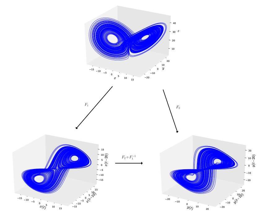
Two variables $y$ and $z$ are coupled if they belong to the same dynamical system. With this notion of coupling in mind, let us consider time delay embeddings of $y$ and $z$ given by Eqs. (5) and (6). $\mathbf{x}$ is expressed in terms of $\mathbf{y}$ in Eq. (5) as

$$\mathbf{x}=F_{1}^{-1}(\mathbf{y})\leavevmode\nobreak\ .$$ (7)

Putting the above in Eq. (6) yields:

$$\mathbf{z}=(F_{2}\circ F_{1}^{-1})(\mathbf{y})\leavevmode\nobreak\ .$$ (8)

Since $F_{2}$ and $F_{1}^{-1}$ are continuous, their composition $F_{2}\circ F_{1}^{-1}$ is also continuous. Please see Appendix A for proof of this. This implies that if $y$ and $z$ belong to the same dynamical system, their exists a continuous function map between their suitable time delay embeddings. Thus,

$$\mathbf{z}=\Psi(\mathbf{y})$$ (9)

where $\Psi=F_{2}\circ F_{1}^{-1}$ is continuous. It is easy to see that $y$ and $z$ above are inter-changeable. The concept is illustrated in Fig. 1 which shows the Lorenz attractor along with time delay embeddings using $x$ and $y$ variables of this system. A continuous functional map $F_{1}$ exists between the original attractor and the time delay embedding with the $x$ variable. Similarly, a continuous $F_{2}$ exists for the embedding with the $y$ variable. This implies that a continuous map $F_{2}\circ F_{1}^{-1}$ also exists between embeddings of $x$ and $y$.

II Statistics to assess the necessary condition

Consider a point $\mathbf{y}_{c}$ on the reconstructed manifold for variable $y$. Let this point be mapped to $\mathbf{z}_{c}$ by $\Psi$. If $\Psi$ is continuous at the point $\mathbf{y}_{c}$ then for every $\epsilon>0$ there exists a $\delta>0$ such that for all $\mathbf{y}$:

$$\left|\mathbf{y}-\mathbf{y}_{c}\right| <\delta\Rightarrow\left|\Psi(\mathbf{y})-\Psi(\mathbf{y}_{c})\right|<\epsilon$$

or

$$\left|\mathbf{y}-\mathbf{y}_{c}\right| <\delta\Rightarrow\left|\mathbf{z}-\mathbf{z}_{c}\right|<\epsilon\leavevmode\nobreak\ .$$ (10)

Consider two time series of $y(t)$ and $z(t)$ of equal length $N$. Consider embeddings of $\mathbf{y},\leavevmode\nobreak\ \mathbf{z}$ of $y(t)$ and $z(t)$ respectively. Let their exist a map $\mathbf{z}=\Psi(\mathbf{y})$ between $\mathbf{y}$ and $\mathbf{z}$. Consider a point $\mathbf{y}_{c}$ on the embedding $\mathbf{y}$. Let this point be mapped to $\mathbf{z}_{c}$ by $\Psi$. Consider a ball of size $\epsilon$ centered around $\mathbf{z_{c}}$. Let their be $n_{\epsilon}$ number of points inside this ball. Consider a ball of minimum size $\delta$ centered around $\mathbf{y_{c}}$ such that all points within this ball are mapped by $\Psi$ to points within the $\epsilon$ ball. $\delta$ can be found by starting from small values and gradually increasing it until the above condition is satisfied. Let there be $n_{\delta}$ number of points within the $\delta$ ball.

The probability $p_{\epsilon}$ of point from $\mathbf{y}$ space being mapped into the $\epsilon$ ball by random chance is

$$p_{\epsilon}=\frac{n_{\epsilon}}{N}\leavevmode\nobreak\ .$$ (11)

The probability of $k$ successful draws out of $n_{\delta}$ points drawn from a sample of size $N$ with probability of success for each draw being $p_{\epsilon}$ is given by the binomial distribution:

$$p(k)=\frac{n_{\delta}!}{k!(n_{\delta}-k)\leavevmode\nobreak\ !}p_{\epsilon}^{k}\left(1-p_{\epsilon}\right)^{n_{\delta}-k}\leavevmode\nobreak\ .$$ (12)

This is also the probability of getting $k$ number of heads out of $n_{\delta}$ tosses of a coin where the probability of getting a head in each toss is $p_{\epsilon}$. Our null hypothesis for continuity is that $n_{\delta}$ points inside the $\delta$ are mapped into the $\epsilon$ ball by random chancePecora1 . The probability $p_{\delta}$ of all $n_{\delta}$ points inside the $\delta$ ball landing into the $\epsilon$ ball by random chance is

$$p_{\delta}=p_{\epsilon}^{n_{\delta}}\leavevmode\nobreak\ .$$ (13)

This event lies in the tail of the distribution given by Eq. (12). The above value should be small relative to the maximum probability of such an event, $p_{max}$, in order to reject the null hypothesis. The likelihood of this event happening is defined as $\frac{p_{\delta}}{p_{max}}$ where

$$p_{max}=\operatorname*{arg\,max}_{k}p(k)\leavevmode\nobreak\ .$$ (14)

Thus, the statistic for continuity is thus defined as:

$$\theta(\epsilon,\mathbf{y}_{c})=1-\frac{p_{\delta}}{p_{max}}\leavevmode\nobreak\ .$$ (15)

$\theta(\epsilon,\mathbf{y}_{c})$ is bounded below by 0 and bounded above by 1. If the value of $\theta(\epsilon,\mathbf{y}_{c})$ is high, then the function is continuous at $\mathbf{y}_{c}$. Let $d$ be the length of the diagonal of the bounding box for the $\mathbf{z}$ attractor. $\epsilon$ can then be expressed in terms of a fraction of $d$ as

$$\epsilon=\epsilon_{f}d$$ (16)

where $0\leq\epsilon_{f}\leq 1$. The value of $\theta$ is averaged over all the sample points and can be expressed as

$$\theta_{avg}(\epsilon_{f})=\frac{1}{N}\sum_{i=1}^{N}\theta(\epsilon_{f},\mathbf{y}_{i})\leavevmode\nobreak\ .$$ (17)

$\theta_{avg}(\epsilon_{f})$ above represents the measure of coupling being proposed in this paper and will be referred to as the coupling statistic in the remainder of this paper.

III Forward causality: Determining the Markov order

A time series $x_{t}$ $(t=1,2,...,N)$ is an $n^{th}$ order Markov process if the probability of $x_{t+1}$, conditioned on all the previous values of $x$ in time, is independent of $x_{t-m-1}$ where $m>n$. This can written as

$$p(x_{t+1}|x_{t},x_{t-1},...,x_{1})=p(x_{t+1}|x_{t},x_{t-1},...,x_{t-n-1})\leavevmode\nobreak\ .$$ (18)

$x_{t-m-1}$ where $m>n$ are irrelevant in determining the transition probability. The same has been termed as irrelevancy in Ref. Casdagli . Irrelevancy is an important concept and is fundamental to time series modeling but has received very little attention in the literature. Causality for all practical purposes is lost beyond a certain time in the past. Events beyond a time limit in the past do not have any bearing on the future states.

The Markov order is determined by examining how well conditioned the future states are given a certain Markov order $n$. With a proper choice of Markov order $n$, the variance of future values of $x$, conditioned on the present, would be minimized. The variance of $x(t+T)$ for a small sized ball $B_{r}(\mathbf{x}(t))$ of radius $r$ around $\mathbf{x}\in R^{n}$, normalized by the size of the ball, is given by

$$\sigma_{r}^{2}(T,\mathbf{x}(t))=\frac{1}{r^{2}}Var(x(t+T)|B_{r}(\mathbf{x}(t)))\leavevmode\nobreak\ .$$ (19)

Uzal et alUzal modified the above by taking the integral of the $\sigma_{r}^{2}(T,\mathbf{x}(t))$ from zero to prediction horizon $T_{M}$:

$$\sigma_{r}^{2}(\mathbf{x})=\frac{1}{T_{M}}\int_{0}^{T_{M}}\sigma_{r}^{2}(T,\mathbf{x})dT\leavevmode\nobreak\ .$$ (20)

Assuming a certain Markov order $m$, $k$ nearest neighbors of $\mathbf{x}(t)$ are considered. Let us denote this set, which includes $\mathbf{x}(t)$ itself, as $U_{k}(\mathbf{x}(t))$. The conditional variance of $x$ at $t+T$ is approximated using these nearest neighbors as

$$E_{k}^{2}(T,\mathbf{x}(t))=\frac{1}{k+1}\operatorname*{\sum}_{x^{\prime}\in U_{k}(\mathbf{x}(t))}\left[x^{\prime}(T)-u_{k}(T,\mathbf{x}(t))\right]^{2}\leavevmode\nobreak\ ,$$ (21)

where $x^{\prime}(T)$ is the future value of $x$ corresponding to $\mathbf{x^{\prime}}$, and

$$u_{k}(T,\mathbf{x}(t))=\frac{1}{k+1}\operatorname*{\sum}_{x^{\prime}\in U_{k}(\mathbf{x}(t))}x^{\prime}(T)\leavevmode\nobreak\ .$$ (22)

The expression in Eq. (21) is averaged up to a prediction horizon $T_{M}$. $E_{k}(\mathbf{x}(t))$ can then be defined without explicit dependence on $T$ as

$$E_{k}^{2}(\mathbf{x}(t))=\frac{1}{p}\operatorname*{\sum}_{j=1}^{p}E_{k}^{2}(T_{j},\mathbf{x}(t))\leavevmode\nobreak\ ,$$ (23)

where the sum is over $p$ sampled times $T_{j}$ in $[0,T_{M}]$. The size of the neighborhood for conditional variance estimation is given by

$$\epsilon_{k}^{2}(\mathbf{x})=\frac{2}{k(k+1)}\operatorname*{\operatorname*{\sum}_{\mathbf{x^{\prime}},\mathbf{x^{\prime\prime}}\in U_{k}(\mathbf{x}(t))}}_{\mathbf{x^{\prime\prime}}\neq\mathbf{x}}\|\mathbf{x^{\prime}}-\mathbf{x^{\prime\prime}}\|^{2}\leavevmode\nobreak\ .$$ (24)

This is a measure of the characteristic radius of $U_{k}(\mathbf{x}(t))$. The noise amplification which is a measure of conditional variance is the given as

$$\sigma_{k}^{2}(\mathbf{x})=\frac{E_{k}^{2}(\mathbf{x})}{\epsilon_{k}^{2}(\mathbf{x})}\leavevmode\nobreak\ .$$ (25)

This is averaged over $N$ points as

$$L_{n}=\log\left(\frac{1}{N}\operatorname*{\sum}_{i=1}^{N}\sigma_{k}^{2}(\mathbf{x_{i}})\right)\leavevmode\nobreak\ .$$ (26)

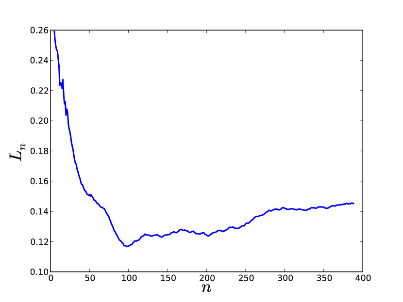
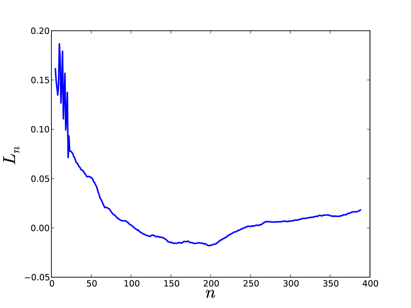
The minimum of the above function with various considered values $n$, would be an appropriate choice for Markov order of the time series. The variation of $L_{n}$ with $n$ will be shown later for an economic time series example in Section VII.

IV Choosing an appropriate embedding

Once the memory of the system is approximated using the procedure elaborated in the previous section, the time series can be embedded onto a much lower dimensional manifold. Markov approximation for deterministic nonlinear dynamics have a strongly perforated structure and the dynamics can be appropriately represented by only a few of the time delay co-ordinatesHolstein . Nearest neighbor searches in dimension greater than 20 can only be done $\mathcal{O}(N^{2})$. A minimal embedding procedure can allow the use of fast search-tree-based methods for the nearest neighbors search. These methods perform a nearest neighbor search operations in $\mathcal{O}(N\log N)$. However, if the data is very noisy and the Markov order is low enough($\mathtt{\sim}\mathcal{O}(20)$), then an embedding with all the delays can be used. The nearest neighbor rank becomes more robust to noise with increasing embedding dimension. It was shown in Ref. hegger2001circuits that the nearest neighbor distance in noisy and noise-free cases are related by the following relationship for a sufficiently high embedding dimension $m$:

$$d_{noisy}^{2}\approx d_{clean}^{2}+2m\xi^{2}\leavevmode\nobreak\ ,$$

where $d_{noisy}$ is the distance in the noisy case, $d_{clean}$ is the distance in the noise-free case and $\xi^{2}$ is the noise variance. Since, the statistics used in this paper depends only on the nearest neighbor ranks and not the actual nearest neighbor distances, it is advisable to use as high an embedding dimension as possible. For a high Markov order case, an approach to minimally embedding the time series on a low dimensional manifold, as described in Ref. Nichkawde , can be used. This methodology recursively chooses delays that maximize derivatives on the project manifold. The objective functional is of the following form:

$$\log\left[\beta_{d}(\tau)\right]=\left<\log\phi^{\prime}_{d_{ij}}\right>\leavevmode\nobreak\ .$$ (27)

In the above equation, $\phi^{\prime}_{d_{ij}}$ is the value of the directional derivative evaluated in the direction from the $i^{th}$ to the $j^{th}$ point of the projected attractor manifold which happens to be the nearest neighbor. The recursive optimization of objective functional given by Eq. (27) eliminates the largest number of false nearest neighbors between successive reconstruction cycles and thus helps achieve an optimal minimal embeddingNichkawde . This procedure would be referred to as MDOP (maximising derivatives on projected manifold). The difference obtained between choosing a minimal embedding versus choosing an embedding with a delay of one and embedding dimension equal to the Markov order will be reported in Section VII.

(a) $\theta_{avg}(\epsilon_{f})$ for probing coupling between $x$ and $y$ variables of Rossler system for noise free case and with noise levels of 1%, 5% and 10%. Coupling can be detected even with 10% Gaussian noise.

(b) $\theta_{avg}(\epsilon_{f})$ for probing coupling between Rossler $x$ and Lorenz $x$.

Figure 2: Coupling statistics for noisy coupled and uncoupled time series.

(a) $\theta_{avg}(\epsilon_{f})$ for $\mathbf{x_{1}}=f_{1}(\mathbf{x_{2}})$ for $\alpha$ of 1, 2, 4, 5, 7, 9 and 16. Mild coupling for $\alpha$ of 1, 2, 4, 5 and 7. The variables become synchronized and fully coupled for $\alpha$ of 9 and 16.

(b) $\theta_{avg}(\epsilon_{f})$ for $\mathbf{x_{2}}=f_{2}(\mathbf{x_{1}})$ for $\alpha$ of 1, 2, 4, 5, 7, 9 and 16. $x_{2}$ drives $x_{1}$ and thus the coupling is unidirectional. The values of $\theta_{avg}(\epsilon_{f})$ is small for $\alpha$ of 1, 2, 4, 5 and 7 as there is no drive from $x_{1}$ to $x_{2}$. The variables however become synchronized for $\alpha$ of 9 and 16 which is manifest as values of $\theta_{avg}(\epsilon_{f})$ close to one. Thus the approach proposed can distinguish between uncoupled and fully synchronized systems.

Figure 3: Coupling between unidirectionally coupled Lorenz systems.

V Coupling statistics for coupled and uncoupled systems

Let us consider the $x$ and $y$ variables of the Rossler systemRossler . This system is modeled by a set of 3 coupled ordinary differential equations

$$\dot{x} =-y-z$$

$$\dot{y} =x+ay$$

$$\dot{z} =b+z(x-c)$$

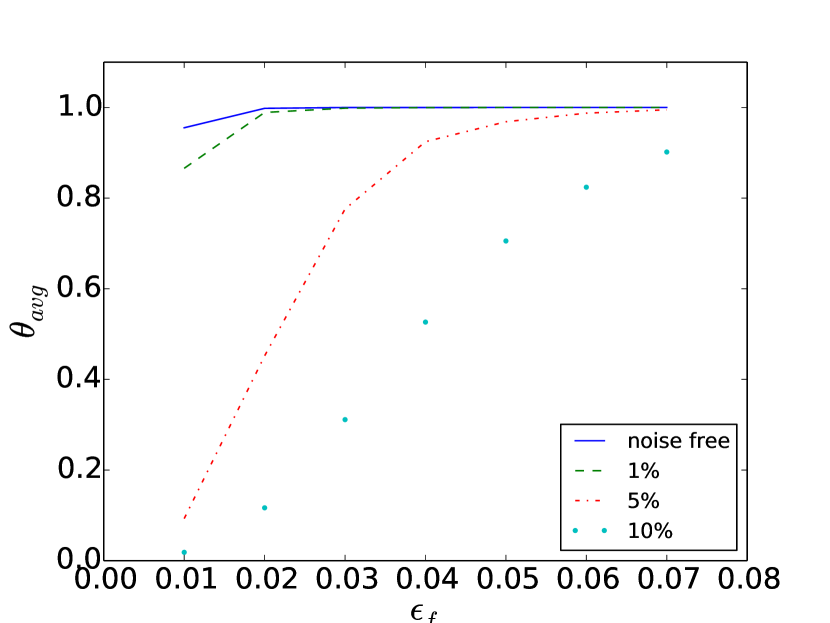
with parameter values $a=0.2,\leavevmode\nobreak\ b=0.2,\leavevmode\nobreak\ c=5.7$. 10000 points were sampled with a $\delta t$ of 0.05 with initial condition $[0.1,0,0]$. Time delays for embedding are determined using the method prescribed in Ref. Nichkawde . Delays of 30 and 17 are found to be most optimal for the $x$ variable whereas delays of 31 and 17 are found to be most optimal for the $y$ variable. $\theta_{avg}$ is evaluated for values of $\epsilon_{f}$ ranging from 0.01 to 0.07. These values are shown in Fig. 2(a) for noise free case and with noise levels of 1%, 5% and 10%. The value $\theta_{avg}$ converges quickly to the expected value of 1 for very small $\epsilon_{f}$ for noise-free and 1% noise cases. Further increase in noise levels degrades the statistics. The coupling can still be easily ascertained for noise levels upto 10%.

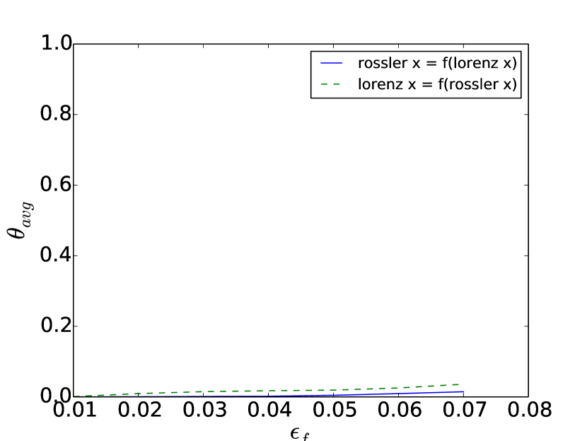
The behavior of coupling statistics for two uncoupled systems is shown in Fig. 2(b). One of the variables is chosen as $x$ variable for Rossler system and is taken same as in the previous example. A time series of equal length is generated for Lorenz system which is given by the following set of equations:

$$\dot{x} =\sigma(y-x)$$

$$\dot{y} =-xz+rx-y$$

$$\dot{z} =xy-\beta z$$

where $\sigma=10,\leavevmode\nobreak\ r=28,\leavevmode\nobreak\ \beta=8.0/3$. The $x$ variable for this system is taken as the second variable. The value of $\theta_{avg}$ for values of $\epsilon_{f}$ ranging from 0.01 to 0.07 are shown in Fig. 2(b). Very low values of the measure is indicative of no coupling between the variables, as expected. The measure is exactly zero when two noise signals are probed for coupling.

VI Directionality and synchronization

The formulation proposed in this paper says nothing about the directionality of the coupling. Nevertheless, the following is still conjectured: Two variables $x_{1}$ and $x_{2}$ are unidirectionally coupled with $x_{2}$ driving $x_{1}$ if the map $\mathbf{x_{1}}=f_{1}(\mathbf{x_{2}})$ between embedding $\mathbf{x_{1}}$ of $x_{1}$ and $\mathbf{x_{2}}$ of $x_{2}$ is continuous, whereas, the map $\mathbf{x_{2}}=f_{2}(\mathbf{x_{1}})$ is not continuous.

The above conjecture is demonstrated using the asymmetrically coupled Lorenz system as an example. The equations for the asymmetrically coupled Lorenz systembelykh2006synchronization are given by

$$\dot{x_{1}} =\sigma(y_{1}-x_{1})+\alpha(x_{2}-x_{1}),\quad\dot{x_{2}}=\sigma(y_{2}-x_{2})$$

$$\dot{y_{1}} =rx_{1}-y_{1}-x_{1}z_{1},\quad\dot{y_{2}}=rx_{2}-y_{2}-x_{2}z_{2}$$

$$\dot{z_{1}} =x_{1}y_{1}-\beta z_{1},\quad\dot{z_{2}}=x_{2}y_{2}-\beta z_{2}$$

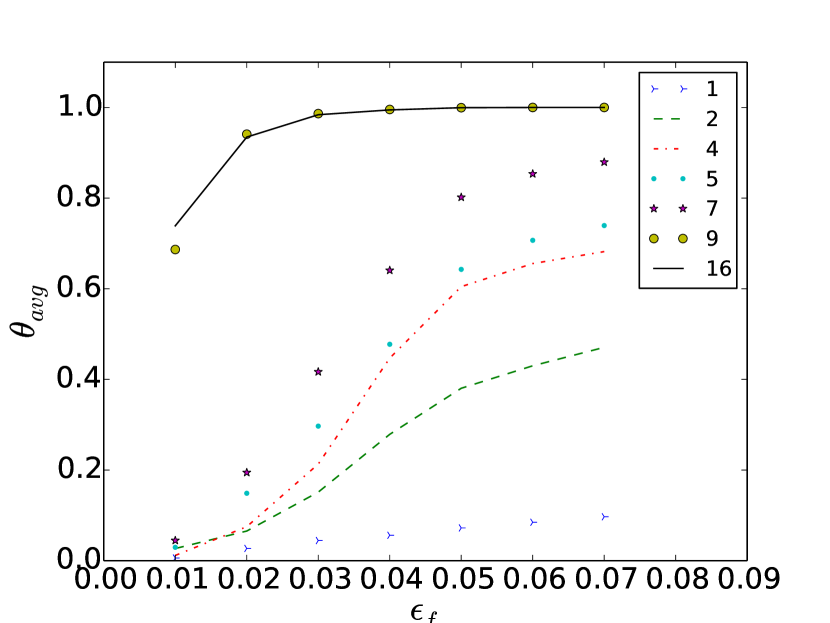
where $\sigma=10,\leavevmode\nobreak\ r=28,\leavevmode\nobreak\ \beta=8.0/3$ and $\alpha$ is the strength of coupling. The above equations represent two different Lorenz systems with the second system driving the first system. The first system is coupled to the second system with the $x_{2}$ variable driving the dynamics of $x_{1}$ via the coupling term $\alpha(x_{2}-x_{1})$. This coupling is asymmetric as the dynamics of the second system represented by $x_{2},\leavevmode\nobreak\ y_{2}$ and $z_{2}$ is independent of the first system represented by variable $x_{1},\leavevmode\nobreak\ y_{1}$ and $z_{1}$.

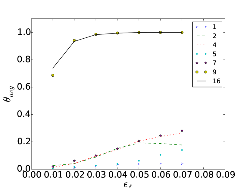
This asymmetric coupling is demonstrated in Fig. 3(a) and 3(b) which shows the values of $\theta_{avg}(\epsilon_{f})$ for various values of coupling strength $\alpha$ for maps $\mathbf{x_{1}}=f_{1}(\mathbf{x_{2}})$ and $\mathbf{x_{2}}=f_{2}(\mathbf{x_{1}})$. The values of $\theta_{avg}(\epsilon_{f})$ for $f_{1}$ and $f_{2}$ for values of 1, 2, 4, 5, 7, 9 and 16 of $\alpha$ are shown. There is almost no coupling for $\alpha=1$ which is reflected in low values in both directions, although even for this case it is higher for $f_{1}$. As conjectured above, the directionality of coupling can easily be seen for values of $\alpha$ of 2, 4, 5 and 7. The systems become fully synchronized for large values of $\alpha$ which manifests as full coupling in both direction as reflected for $\alpha$ of 9 and 16. Transfer entropy is unable to differentiate between no coupling and fully synchronized systemsStaniek as both cases give a value of zero. The present approach clearly differentiates between no coupling and fully synchronized systems. No coupling is manifest as nearly zero values of $\theta_{avg}(\epsilon_{f})$ in both direction. Fully synchronized systems manifest as nearly a value of one for $\theta_{avg}(\epsilon_{f})$ in both direction.

VII Complex time series from the finance world

In this section, the currency exchange rate Canadian Dollar-Japanese Yen and oil prices between 2000 to 2014 are probed for coupling. The coupling between the Canadian Dollar-Japanese Yencanjpy exchange rate and the WTI crude oil pricewti is considered.

Figure 4: Currency exchange rate Canadian Dollar-Japanese Yen and oil price between 1990 to 2013. The values have been rescaled between 0 and 1.

(a) Currency exchange rate Canadian Dollar-Japanese Yen and oil price between 1990 to 2013. A level 7 approximation with Daubechies wavelet filter is also shown superposed. This is subtracted from the original time series in order to analyze the local fluctuation dynamics.

(b) Currency exchange rate local fluctuations after subtracting the wavelet approximation in Fig. 5(a).

Figure 5: Exchange rate detrending using wavelet filter.

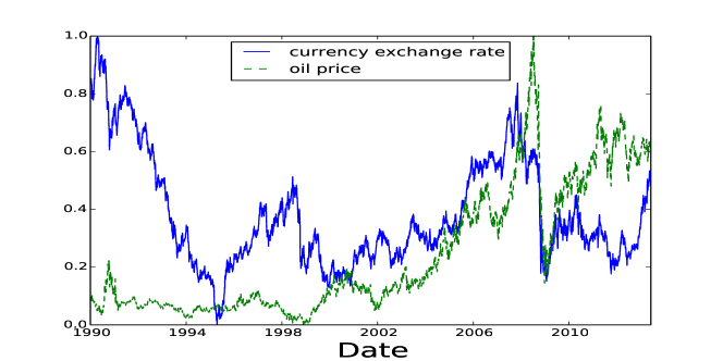
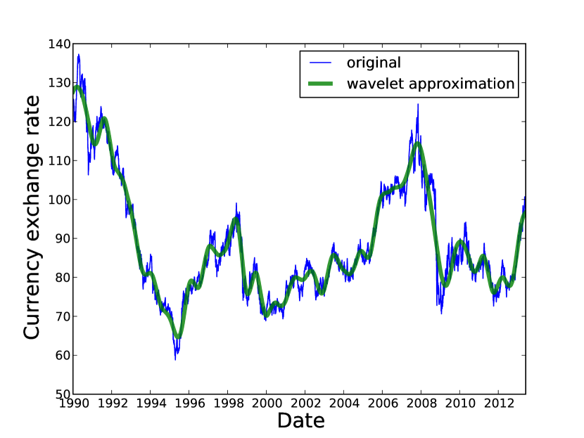
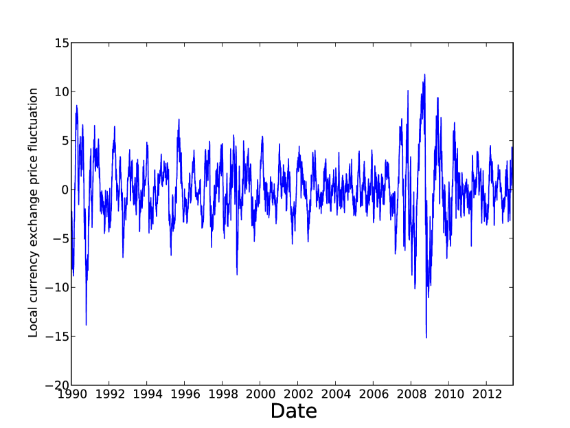
These variables are shown in Fig. 4 for the period 1990 to 2013. The values have been rescaled to take a value between 0 and 1. It is hard to see any evidence of coupling by mere visual inspection. In order to analyze both series for coupling, the series is detrended by using Daubechies wavelet filterdaubechies1990wavelet . The level 7 approximation superimposed on the original time series for currency exchange rate is shown in Fig. 5(a). This approximation is subtracted from the series and local fluctuation dynamics is probed for coupling. The local fluctuation for currency exchange rate is shown in Fig. 5(b). The same procedure is applied to oil price time series. The variation $L_{n}$ with $n$ for currency exchange rate (CER) series and oil price (OP) series is shown in Fig. 6(a) and 6(b) respectively. Markov order of 98 and 198 are found for CER and OP series.

(a) Variation of $L_{n}$ for currency exchange series. The minimum value is obtained for $n=98$ which is taken as Markov order in the state space reconstruction process.

(b) Variation of $L_{n}$ for oil price series. The minimum value is obtained for $n=198$ which is taken as Markov order in the state space reconstruction process.

Figure 6: Markov order for exchange rate and oil price fluctuation dynamics.

Figure 7: State space reconstruction for currency exchange rate local fluctuation dynamics. Delays of 45, 90, 68, 21 and 32 are found to be optimal.

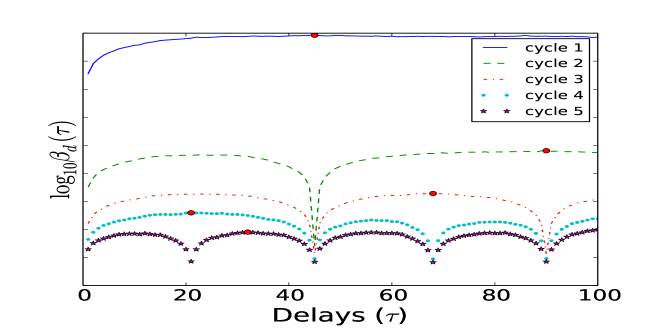
MDOP reconstruction methodology is then applied to these local fluctuation series. The reconstruction for CER is shown in Fig. 7. Delays of 45, 90, 68, 21 and 32 are found to be optimal. Using the same procedure the delays of 155, 190, 37, 64 and 123 were found to be optimal for the oil price fluctuation series.

(a) $\theta_{avg}(\epsilon_{f})$ for probing coupling between Canadian Dollar-Japanese Yen exchange rate and oil price using minimal embedding technique. Strong coupling is found between these two variables.

(b) $\theta_{avg}(\epsilon_{f})$ for probing coupling between Canadian Dollar-Japanese Yen exchange rate and oil price using very high embedding dimension. The measure is seen to be convergent to a value of one indicating strong coupling.

Figure 8: Coupling between exchange rate and oil fluctuation dynamics.

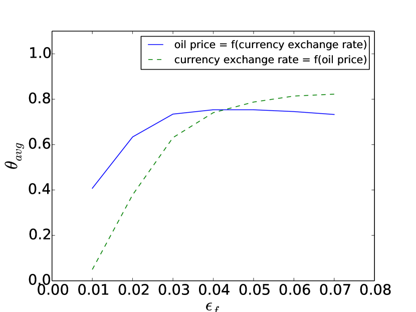
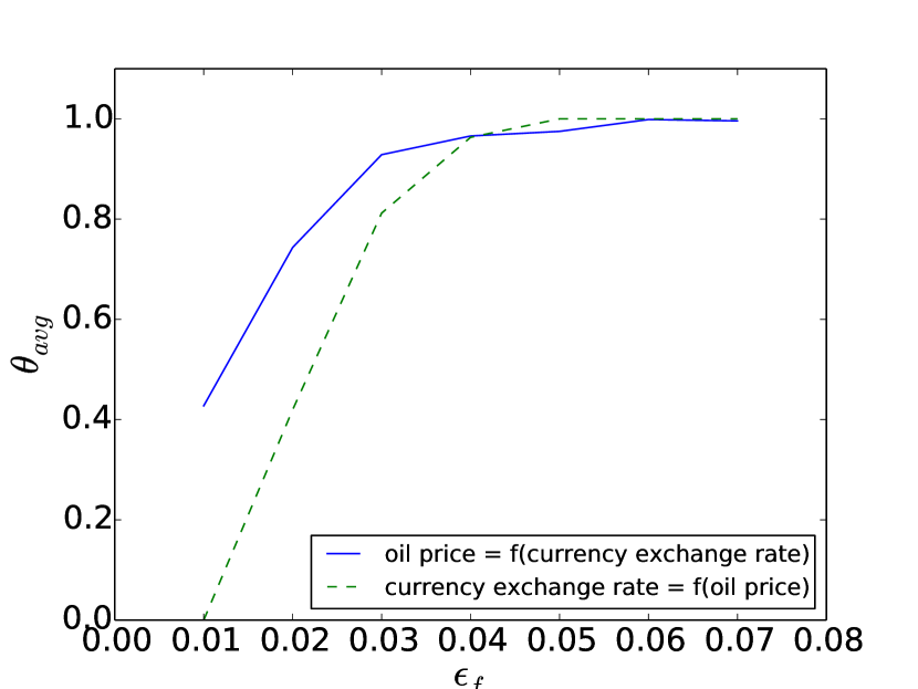
The values of $\theta_{avg}(\epsilon_{f})$ for maps between these embeddings for values of $\epsilon_{f}$ ranging from 0 to 0.07 is shown in Fig. 8(a). The high dimensional embeddings for both series are also considered. Fig. 8(b) shows the values of $\theta_{avg}(\epsilon_{f})$ when embedding dimension equal to Markov order with a time delay of one is used. The time series considered in this case is noisy, and, as described earlier in Section IV, the nearest neighbor ranks become more robust for higher embedding dimension. Since the $\theta_{avg}(\epsilon_{f})$ measure depends only on nearest neighbor rank and not on actual nearest neighbor distance, it is more suitable to use high embedding dimension for noisy cases. This of course comes at the penalty of computational cost because nearest neighbor search is $\mathcal{O}(N^{2})$ operation for dimensions greater than 20 even with fast search algorithms. Strong coupling is evident from values in Figs. 8(a) and 8(b). This example shows the inter-connectedness of economic forces in a complex network.

VIII Conclusions

A physics based measure of coupling has been proposed. The measure assesses the continuity of functional maps between time series embeddings of two variables. It has been shown that it is necessary for the existence of a continuous functional map between suitable time series embeddings of two variables in order for coupling to be established. A mathematical proof for this necessity has been provided. A statistic for continuity, based on first principles definition of continuity, is used to probe for coupling. This measure of continuity of the functional map is convergent to a value of one in the case of coupling and zero in case of no coupling. The proposed approach has been demonstrated by establishing coupling between $x$ and $y$ variables of the Rossler system. The measure is shown to be robust even in the presence of large amount of observational noise. It has also been shown that the proposed approach can also be used to assess the directionality of coupling. The directionality can be determined if the functional map is found to be continuous in one direction and not continuous in other direction. This was demonstrated using unidirectionally coupled Lorenz oscillators. The measure can also distinguish between fully synchronized oscillators and uncoupled systems unlike the information-theoretic measure of transfer entropy which is unable to distinguish between these two cases. The approach is model-free and works very well with high-dimensional signals such as those found in financial settings. Density estimates in transfer entropy is an intractable problem in high dimensions. The methodology presented does not require high-dimensional density estimation. Two disparate economic variables, currency exchange rate between the Canadian Dollar-Japanese Yen and oil prices have been shown to be strongly coupled using this measure.

Appendix A Composition of two continuous function is a continuous function

Definition: A function $F(\mathbf{x})$ is continuous at $\mathbf{x_{c}}$ if for every $\epsilon>0$ there exists a $\delta>0$ such that for all $\mathbf{x}$:

$$\left|\mathbf{x}-\mathbf{x}_{c}\right| <\delta\Rightarrow\left|F(\mathbf{x})-F(\mathbf{x}_{c})\right|<\epsilon\leavevmode\nobreak\ .$$ (28)

Proposition: If two function $F_{1}(\mathbf{x})$ and $F_{2}(\mathbf{x})$ are continuous at $\mathbf{x_{c}}$ then their composition $(F_{1}\circ F_{2})(\mathbf{x})$ is also continuous at $\mathbf{x_{c}}$.

Proof: Let $F_{1}$ and $F_{2}$ be two continuous functions. Consider a point $\mathbf{x}_{c}$. Since $F_{1}$ is continuous, for every $\epsilon>0$ there exists a $\eta>0$ such that for all $\mathbf{x}$:

$$\left|F_{2}(\mathbf{x})-F_{2}(\mathbf{x}_{c})\right| <\eta\Rightarrow\left|(F_{1}\circ F_{2})(\mathbf{x})-(F_{1}\circ F_{2})(\mathbf{x}_{c})\right|<\epsilon\leavevmode\nobreak\ .$$ (29)

Since $F_{2}$ is continuous, for every $\eta>0$ there exists a $\delta>0$ such that for all $\mathbf{x}$:

$$\left|\mathbf{x}-\mathbf{x}_{c}\right| <\delta\Rightarrow\left|F_{2}(\mathbf{x})-F_{2}(\mathbf{x}_{c})\right|<\eta\leavevmode\nobreak\ .$$ (30)

It follows from assertions (29) and (30) that for every $\epsilon>0$ there exists a $\delta>0$ such that for all $\mathbf{x}$:

$$\left|\mathbf{x}-\mathbf{x}_{c}\right| <\delta\Rightarrow\left|(F_{1}\circ F_{2})(\mathbf{x})-(F_{1}\circ F_{2})(\mathbf{x}_{c})\right|<\epsilon\leavevmode\nobreak\ .$$

It thus follows from definition (28) that the composition function $(F_{1}\circ F_{2})(\mathbf{x})$ is continuous at $\mathbf{x}_{c}$.