Quantum Gate Generation by $T$-Sampling Stabilization

Abstract

This paper considers right-invariant and controllable driftless quantum systems with state $X(t)$ evolving on the unitary group $\mbox{U}(n)$ and $m$ inputs $u=(u_{1},\dots,u_{m})$. The $T$-sampling stabilization problem is introduced and solved: given any initial condition $X_{0}$ and any goal state $X_{goal}$, find a control law $u=u(X,t)$ such that $\lim_{j\to\infty}X(jT)=X_{goal}$ for the closed-loop system. The purpose is to generate arbitrary quantum gates corresponding to $X_{goal}$. This is achieved by the tracking of $T$-periodic reference trajectories $(\overline{X}_{\mathbf{a}}(t),\overline{u}_{\mathbf{a}}(t))$ of the quantum system that pass by $X_{goal}$ using the framework of Coron’s Return Method. The $T$-periodic reference trajectories $\overline{X}_{\mathbf{a}}(t)$ are generated by applying controls $\overline{u}_{\mathbf{a}}(t)$ that are a sum of a finite number $M$ of harmonics of $\sin(2\pi t/T)$, whose amplitudes are parameterized by a vector $\mathbf{a}$. The main result establishes that, for $M$ big enough, $X(jT)$ exponentially converges towards $X_{goal}$ for almost all fixed $\mathbf{a}$, with explicit and completely constructive control laws. This paper also establishes a stochastic version of this deterministic control law. The key idea is to randomly choose a different parameter vector of control amplitudes $\mathbf{a}=\mathbf{a}_{j}$ at each $t=jT$, and keeping it fixed for $t\in[jT,(j+1)T)$. It is shown in the paper that $X(jT)$ exponentially converges towards $X_{goal}$ almost surely. Simulation results have indicated that the convergence speed of $X(jT)$ may be significantly improved with such stochastic technique. This is illustrated in the generation of the C–NOT quantum logic gate on $\mbox{U}(4)$.

Keywords:

controllable right-invariant driftless systems; Coron’s Return Method; LaSalle’s invariance theorem; quantum control; unitary group; stochastic stability.

1 Introduction

Consider a nonlinear driftless system of the form

$$\dot{X}(t)=\sum_{k=1}^{m}u_{k}(t)g_{k}(X(t)),\quad X(0)=X_{0},$$ (1)

where $X$ is the state and $u=(u_{1},\dots,u_{m})$ is the control, and assume that $X_{goal}$ is a given goal state. The following problem is introduced in this paper:

Definition 1.

($T$-sampling stabilization problem) Given an initial condition $X_{0}$, find a control law $u=u(X,t)$ such that $\lim_{j\to\infty}X(jT)=X_{goal}$ for the closed-loop system.

The reason for considering such relaxed version of the stabilization problem relies on the known obstructions that arises in the context of driftless systems [1, 17]. However, it is possible to stabilize such systems by means of smooth time-varying feedbacks that are time-periodic [3, 17], but exponential convergence is impossible with such smooth control law. For the less restrictive $T$-sampling stabilization problem, this paper proves that exponential convergence can be obtained.

In this work one solves the $T$-stabilization problem for controllable right-invariant driftless quantum models evolving on $\mbox{U}(n)$. The purpose is to generate arbitrary quantum gates corresponding to $X_{goal}$. For this end, one considers the tracking of $T$-periodic reference trajectories $(\overline{X}_{\mathbf{a}}(t),\overline{u}_{\mathbf{a}}(t))$ of system (1) that pass by $X_{goal}$ using the framework of Coron’s Return Method [3] (see also [5, 6]). The $T$-periodic reference trajectories $\overline{X}_{\mathbf{a}}(t)$ are generated by applying controls $\overline{u}_{\mathbf{a}}(t)$ that are a sum of a finite number $M$ of harmonics of $\sin(2\pi t/T)$, whose amplitudes are parameterized by a vector $\mathbf{a}$. The main deterministic result shows that, for $M$ big enough, $X(jT)$ exponentially converges towards $X_{goal}$ for almost all fixed $\mathbf{a}$, with explicit and completely constructive control laws. A new Lyapunov function $\mathcal{V}$ that is inspired in a homographic function is introduced. The advantage of such $\mathcal{V}$ with respect to the standard fidelity functions, is that $\mathcal{V}$ decreases without singularities and with no nontrivial LaSalle’s invariants, which is an advantage when compared with other previous results in the literature [9, 20, 21]. The key ingredients of the stability proof is the $T$-periodic version of LaSalle’s theorem [13], Coron’s Return Method [3] and the stabilization techniques of [10].

This paper also establishes a stochastic version of the deterministic control law described above. This is achieved by randomly choosing a different amplitudes vector $\mathbf{a}=\mathbf{a}_{j}$ at each $t=jT$, and keeping it fixed for $t\in[jT,(j+1)T)$. The main stochastic result shows that $X(jT)$ converges exponentially towards $X_{goal}$ almost surely. The proof relies on a well-known stochastic version of LaSalle’s theorem [12]. Simulation results have indicated that the convergence speed of $X(jT)$ may be significantly improved with such stochastic technique.

The deterministic and the stochastic methods described above are both local in nature, since they require that $X_{goal}$ must not have any eigenvalue equal to $-1$. However, it is shown that the $T$-stabilization problem may be easily solved globally in a two-step procedure. Furthermore, if one admits a global phase change of $X_{goal}$, which is transparent for quantum systems, then the proposed strategy becomes a global exponential solution of the $T$-sampling stabilization problem.

It follows from the principles of quantum mechanics (in the Copenhagen interpretation) that the (deterministic) Schrödinger equation that governs its dynamics is valid as long as the system remains isolated from external measurements. More precisely, a measurement causes a collapse in (reduction of) the state of the system, and the relation between the state at the moment of a measurement and the one immediately after it can no longer be deduced from the Schrödinger equation, but only in a probabilistic manner by the Projection Postulate (see e.g. [24]). Therefore, feedback control techniques cannot be directly applied. However, it is possible to perform a computer simulation, and then apply the recorded inputs in the real quantum system as being an open-loop control. In the case of quantum systems consisting of $n$-qubits, the present method allows one to generate, in an approximate manner, arbitrary quantum logic gates that operate on $n$-qubits.

The $T$-sampling stabilization control problem here treated for driftless systems of the form (1) evolving on $\mbox{U}(n)$ can be regarded as a generalization of the motion planning control problem. The latter was considered for systems evolving on SU(n) in [23] using optimal control theory, solved in an approximate manner in [14] based on averaging techniques (see also [19] for the case of quantum systems) and treated in [16] for a single qubit quantum system that evolves on $\mbox{SU}(2)$ by means of a flatness approach. Based on decompositions of the Lie group $\mbox{SU}(n)$, [7] (see also the references therein) considers the problem of finding piecewise-constant inputs that steer the state of quantum systems of the form (1) with a drift term to an arbitrary final state $X_{f}\in\mbox{SU}(n)$ in some finite instant of time. It also treats the problem of reaching a given final state in minimum time.

The paper is organized as follows. Section 2.1 develops the proposed solution for the $T$-sampling stabilization problem of controllable driftless quantum systems evolving on $\mbox{U}(n)$. The deterministic and stochastic control laws are exhibited in Sections 2.1 and 2.2, respectively. Section 2.3 exhibits the obtained simulation results in the generation of the C–NOT (Controlled-NOT) quantum logic gate for a quantum system evolving on $\mbox{U}(4)$ ($n=4$). A comparison between the deterministic and the stochastic control strategies is presented. The main deterministic and stochastic results are given in Section 2.4, and their proofs are developed in Section 2.5 and 2.6, respectively. Section 2.7 shows that the convergence of both methods, deterministic and stochastic, are exponential. The conclusions are stated in Section 3. Finally, some proofs and intermediate results were deferred to Appendix.

2 $T$-Sampling Stabilization of Quantum Models

Consider a right-invariant and controllable driftless (homogeneous) quantum system of the form

$$\dot{X}(t)=-\iota\sum_{k=1}^{m}u_{k}(t)H_{k}X(t)=\sum_{k=1}^{m}u_{k}(t)S_{k}X(t),$$ (2)

where $X\in\mbox{U}(n)$ is the state, $\iota\in\mathbb{C}$ is the imaginary unit, $S_{k}=-\iota H_{k}\in\mathfrak{u}(n)$, $\mathfrak{u}(n)$ is the Lie algebra associated to the special unitary group $\mbox{U}(n)$, $u_{k}\in\mathbb{R}$ are the controls and $I$ is the identity matrix. The approach for solving the $T$-sampling stabilization problem on $\mbox{U}(n)$ for system (2) is described as follows. Given any initial condition $X(0)=X_{0}\in\mbox{U}(n)$ in (2), any goal state $X_{goal}\in\mbox{U}(n)$ and any $T>0$, find a smooth $T$-periodic reference trajectory $\overline{X}$: $\mathbb{R}_{+}\rightarrow\mbox{U}(n)$ with $\overline{X}(0)=X_{goal}$, and determine piecewise-smooth control laws $u_{k}$: $\mathbb{R}_{+}\rightarrow\mathbb{R}$, $k=1,\dots,m$, in a manner that

$$\lim_{t\rightarrow\infty}\widetilde{X}(t)=\lim_{t\rightarrow\infty}\overline{X}^{\dagger}(t)X(t)=I.$$ (3)

This is illustrated in Figure 1. In particular, for the sequence of samples $X(jT)$ one has

$$\lim_{j\rightarrow\infty}X(jT)=X_{goal},$$ (4)

and $T$-sampling stabilization is achieved.

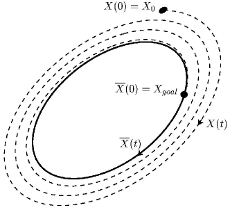
Figure 1: Proposed approach to solve the $T$-sampling stabilization problem.

One denotes by $\mathbb{N}$ the set of natural numbers (including zero), by $\mathbb{C}^{n\times n}$ the real Banach space of $n\times n$-square matrices with complex entries endowed with the Frobenius norm $\|\cdot\|$, and by $\mbox{Tr}(X)$ the trace of $X\in\mathbb{C}^{n\times n}$. If $X\in\mathbb{C}^{n\times n}$ and $\Omega\subset\mathbb{C}^{n\times n}$ is nonempty, $d(X,\Omega)\triangleq\inf_{Y\in\Omega}\|Y-X\|$. The Lie algebra generated by the $S_{k}$’s in (2) is denoted as $\mbox{Lie}\{S_{1},\dots,S_{m}\}$. For simplicity, it will be assumed throughout this paper that $n\geq 1$, $T>0$ and the goal state $X_{goal}\in\mbox{U}(n)$ are fixed. Moreover, unless otherwise stated, one assumes that the initial condition of (2) is $X(0)=X_{0}$, where $X_{0}\in\mbox{U}(n)$ is arbitrary but fixed. The controllability assumption means that the Lie algebra generated by the $S_{k}$’s in (2) coincides with $\mathfrak{u}(n)$ [11].

2.1 Deterministic Control Laws

Consider system (2). Take $T>0$ and set $\omega=2\pi/T$. Fix an integer $M>0$ and choose $a_{k,\ell}\in\mathbb{R}$ for $k=1,\dots,m$, $\ell=1,\dots,M$. Consider the $T$-periodic continuous reference controls

$$\overline{u}_{k}(t)=\sum_{\ell=1}^{M}a_{k,\ell}\sin(\ell\omega t),\quad t\in\mathbb{R},\;k=1,\dots,m,$$ (5)

and the associated reference trajectory $\overline{X}(t)\in\mbox{U}(n)$, $t\in\mathbb{R}$, solution of

$$\dot{\overline{X}}(t)=\sum_{k=1}^{m}\overline{u}_{k}(t)S_{k}\overline{X}(t),\quad\overline{X}(0)=X_{goal}\in\mbox{U}(n).$$ (6)

This means that $\overline{X}(t)$ is the solution of (2) with $u_{k}=\overline{u}_{k}$ and initial condition $X_{goal}$ at $t=0$. Since $\overline{u}_{k}(T-t)=-\overline{u}_{k}(t)$ for $t\in\mathbb{R}$, one has $\overline{X}(t)=\overline{X}(T-t)$ for $t\in\mathbb{R}$, and thus $\overline{X}(jT)=X_{goal}$ for all $j\geq 0$ (see [6] for details). Therefore, $\overline{X}(t)$ is $T$-periodic.

The tracking error $\widetilde{X}(t)=\overline{X}^{{\dagger}}(t)X(t)$ obeys

$$\dot{\widetilde{X}}(t)=\sum_{k=1}^{m}\widetilde{u}_{k}(t)\widetilde{S}_{k}(t)\widetilde{X}(t),\quad\widetilde{X}(0)=X_{goal},$$ (7)

where $\widetilde{u}_{k}=u_{k}-\overline{u}_{k}$, and $\widetilde{S}_{k}(t)=\overline{X}^{{\dagger}}(t)S_{k}\overline{X}(t)\in\mathfrak{u}(n)$ depends on $t\in\mathbb{R}$ and is $T$-periodic. The goal is to stabilize $\widetilde{X}$ towards the identity $I$. In order to accomplish this, one will choose a suitable Lyapunov function $\mathcal{V}(\widetilde{X})$ to measure the distance from $\widetilde{X}$ to the identity matrix $I$.

Let $\mathcal{W}\subset\mbox{U}(n)$ be the set of $\widetilde{X}\in\mbox{U}(n)$ which have all the eigenvalues different from $-1$. Note that

$$\mathcal{W}=\{W\in\mbox{U}(n)\;|\;\det(I+W)\neq 0\}.$$ (8)

By the continuity of the determinant function, it follows that $\mathcal{W}$ is open in $\mbox{U}(n)$. Denote by $\mathbf{H}$ the (real) vector space of all Hermitian $n$-square complex matrices and consider the map

$$\mathcal{W}\ni\widetilde{X}\mapsto\Upsilon(\widetilde{X})=\iota\frac{\widetilde{X}-I}{\widetilde{X}+I}\in\mathbf{H}.$$

One has that $\Upsilon$: $\mathcal{W}\rightarrow\mathbf{H}$ is a well-defined smooth map on the open submanifold $\mathcal{W}$ of $\mbox{U}(n)$. Indeed, writing

$$\Upsilon(\widetilde{X})=\iota\dfrac{\widetilde{X}-\widetilde{X}^{{\dagger}}\widetilde{X}}{\widetilde{X}+\widetilde{X}^{{\dagger}}\widetilde{X}},$$

one gets

$$\Upsilon(\widetilde{X})^{{\dagger}} =-\iota\dfrac{\widetilde{X}^{{\dagger}}-\widetilde{X}\widetilde{X}^{{\dagger}}}{\widetilde{X}^{{\dagger}}+\widetilde{X}\widetilde{X}^{{\dagger}}}=-\iota(I-\widetilde{X})\widetilde{X}^{{\dagger}}((I+\widetilde{X})\widetilde{X}^{{\dagger}})^{-1}=\Upsilon(\widetilde{X}).$$

For $\widetilde{X}\in\mathcal{W}$, the distance to $I$ is measured by the Frobenius norm of $\Upsilon(\widetilde{X})$:

$$\mathcal{V}(\widetilde{X})\triangleq\mbox{Tr}\left(\Upsilon(\widetilde{X})\Upsilon(\widetilde{X})^{{\dagger}}\right)=-\mbox{Tr}\left(\dfrac{(\widetilde{X}-I)^{2}}{(\widetilde{X}+I)^{2}}\right)\geq 0.$$ (9)

Note that $\mathcal{V}$: $\mathcal{W}\rightarrow\mathbb{R}$ is smooth and non-negative. Moreover, $\mathcal{V}(\widetilde{X})=0$ implies $\widetilde{X}=I$. One will impose that $\dot{\mathcal{V}}\leq 0$. Using $\mbox{Tr}(AB)=\mbox{Tr}(BA)$, standard computations yield, for $(\widetilde{X},t)\in\mathcal{W}\times\mathbb{R}$,

$$\dot{\mathcal{V}}(\widetilde{X},t)\triangleq\dfrac{d}{dt}\mathcal{V}(\widetilde{X})=-4\sum_{k=1}^{m}\widetilde{u}_{k}\mbox{Tr}\left(\widetilde{X}(\widetilde{X}-I)(\widetilde{X}+I)^{-3}\widetilde{S}_{k}(t)\right).$$

Choose any (constant) feedback gains $f_{k}>0$. Since $\widetilde{X}(\widetilde{X}-I)(\widetilde{X}+I)^{-3}$ is skew-Hermitian because $\widetilde{X}$ is unitary, $\mbox{Tr}\left(\widetilde{X}(\widetilde{X}-I)(\widetilde{X}+I)^{-3}\widetilde{S}_{k}(t)\right)$ is real for each $k$ and the feedbacks

$$\widetilde{u}_{k}(\widetilde{X},t)=f_{k}\mbox{Tr}\left(\widetilde{X}(\widetilde{X}-I)(\widetilde{X}+I)^{-3}\widetilde{S}_{k}(t)\right)$$ (10)

produce

$$\dot{\mathcal{V}}(\widetilde{X},t)=-4\sum_{k=1}^{m}f_{k}\mbox{Tr}^{2}\left(\widetilde{X}(\widetilde{X}-I)(\widetilde{X}+I)^{-3}\widetilde{S}_{k}(t)\right)=-4\sum_{k=1}^{m}\frac{\widetilde{u}^{2}_{k}(\widetilde{X},t)}{f_{k}}\leq 0,$$ (11)

$(\widetilde{X},t)\in\mathcal{W}\times\mathbb{R}$, and hence ensure that $\mathcal{V}(\widetilde{X}(t))$ is non-increasing. Note that, for the initial condition $\widetilde{X}(0)=\widetilde{X}_{goal}\in\mathcal{W}$, the corresponding solution $\widetilde{X}(t)\in\mathcal{W}$ is defined for every $t\geq 0$. Indeed, since $\mathcal{V}$ is decreasing, the trajectory $\widetilde{X}(t)$ of the closed-loop system (7,10) remains in the positively invariant set $K$ given by

$$K=\{\widetilde{X}\in\mathcal{W}\;|\;\mathcal{V}(\widetilde{X})\leq\mathcal{V}(X_{goal})\},$$ (12)

at least in the maximal interval $[0,t_{max})$ where this solution is defined. Since $K$ is compact (see Appendix A), it follows from well-known results on ordinary differential equations that one cannot have finite time scape, and thus the solution $\widetilde{X}(t)$ is well-defined for all $t\geq 0$.

The controls $\widetilde{u}_{k}(t)=\widetilde{u}_{k}(\widetilde{X}(t),t)$ are defined for all $t\geq 0$, and they are also uniformly bounded on $\mathbb{R}_{+}$, since $\widetilde{X}(t)$ evolves in the compact set $K\subset\mathcal{W}$, the map $\mathcal{W}\ni\widetilde{X}\mapsto\widetilde{X}(\widetilde{X}-I)(\widetilde{X}+I)^{-3}\in\mathbb{C}^{n\times n}$ is smooth, and $\widetilde{S}_{k}(t)$ is $T$-periodic (and thus is bounded). Note that $f_{k}>0,k=1,\ldots,m$, can be seen as “feedback gains” in the expression of $\widetilde{u}_{k}$ above.

The corresponding deterministic control laws are given as

$$u_{k}(X,t)=\overline{u}_{k}(t)+\widetilde{u}_{k}(X,t)=\sum_{\ell=1}^{M}a_{k,\ell}\sin(\ell\omega t)+f_{k}\mbox{Tr}\left(X(\overline{X}^{{\dagger}}(t)X-I)(\overline{X}^{{\dagger}}(t)X+I)^{-3}\overline{X}^{{\dagger}}(t)S_{k}\right)$$ (13)

2.2 Stochastic Control Laws

At the time instants $t=jT,j\in\mathbb{N}$, one chooses the amplitudes $a_{k,\ell}^{j}$ of the reference controls $\overline{u}_{k}(t)$ in (5) for $t\in[jT,(j+1)T)$ in an independent stochastic manner following a uniform distribution on the interval $[-\frac{a_{max}}{2},\frac{a_{max}}{2}]$, where $a_{max}>0$ is arbitrarily fixed. More precisely, assume the Lebesgue probability measure on $\mathbf{A}=[-\frac{a_{max}}{2},\frac{a_{max}}{2}]^{mM}$ (with the Borel algebra). An element $\mathbf{a}_{j}=(a_{k,\ell}^{j})=(a_{1,1}^{j},\dots,a_{1,M}^{j},\dots,a_{m1}^{j},\dots,a_{mM}^{j})\in\mathbf{A}$ gathers the random amplitudes $a_{k,\ell}^{j}\in[-\frac{a_{max}}{2},\frac{a_{max}}{2}]$ of the reference controls $\overline{u}_{k}(t)$ in (5) for $t\in[jT,(j+1)T)$. Fix any i.i.d. (independent and identically distributed) random vectors $\mathbf{a}_{j}=(a_{k,\ell}^{j})$: $\mathbb{N}\rightarrow\mathbf{A}\subset\mathbb{R}^{mM}$ having a uniform distribution on $\mathbf{A}$. The resulting bounded continuous reference controls for $k=1,\ldots,m$ are

$$\overline{u}_{k}(t)=\sum_{\ell=1}^{M}a_{k,l}^{j}\sin(\ell\omega t),\quad t\in[jT,(j+1)T),\;j\in\mathbb{N}.$$ (14)

The corresponding stochastic control laws are given as

$$u_{k}(X,t)=\overline{u}_{k}(t)+\widetilde{u}_{k}(X,t)=\sum_{\ell=1}^{M}a_{k,l}^{j}\sin(\ell\omega t)+f_{k}\mbox{Tr}\left(X(\overline{X}^{{\dagger}}(t)X-I)(\overline{X}^{{\dagger}}(t)X+I)^{-3}\overline{X}^{{\dagger}}(t)S_{k}\right).$$ (15)

2.3 Application to Quantum Control

This section exhibits the simulation results obtained when the deterministic and stochastic control laws were applied in the generation of the C–NOT (Controlled-NOT) quantum logic gate on $\mbox{U}(4)$ and involving two qubits. Thus the underlying Hilbert space corresponds to the tensor product $\mathbb{C}^{2}\otimes\mathbb{C}^{2}\equiv\mathbb{C}^{4}$, each $\mathbb{C}^{2}$ being the Hilbert space of one qubit. We assume here that the dynamics is governed by the

following driftless system of the form (2) with $n=4$ and $m=6$,

$$\dot{X}(t)=-\iota\sum_{k=1}^{6}u_{k}(t)H_{k}X(t),$$

where

$$H_{1}=\sigma_{x}\otimes I_{2},H_{2}=I_{2}\otimes\sigma_{x},H_{3}=\sigma_{y}\otimes I_{2},H_{4}=I_{2}\otimes\sigma_{y},H_{5}=\sigma_{x}\otimes\sigma_{x}+\sigma_{y}\otimes\sigma_{y}+\sigma_{z}\otimes\sigma_{z},H_{6}=I_{2}\otimes I_{2},$$

$\sigma_{x},\sigma_{y},\sigma_{z}\in\mathbb{C}^{2\times 2}$ are the usual Pauli matrices, $\otimes$ is the tensor product, and $I_{2}\in\mathbb{C}^{2\times 2}$ is the 2-identity matrix. It can be shown that this system is controllable (and only Lie brackets of up to length 3 are required). The aim is to generate two distinct goal matrices:

$$X_{1_{goal}}=\exp(\iota\pi/2)\left[\begin{array}[]{cccr}1&0&0&0\\ 0&1&0&0\\ 0&0&0&1\\ 0&0&1&0\end{array}\right],\qquad X_{2_{goal}}=\left[\begin{array}[]{ccrc}1&0&0&0\\ 0&0&-1&0\\ 0&1&0&0\\ 0&0&0&1\end{array}\right].$$

The first goal propagator, up to the irrelevant global phase $e^{i\pi/2}$, corresponds to a C–NOT gate which is fundamental in quantum computation [15]. The second one was chosen for academic purposes. Note that $X_{1_{goal}},X_{2_{goal}}\in\mathcal{W}$. Some $\mbox{MATLAB}^{\circledR}$ simulations have been done with this system, implementing both deterministic (13) and stochastic (15) control laws. One has chosen $M=4$, $a_{max}=0.25$, $f_{k}=Ma_{max}=0.75$ and $T=25$ for all simulations. For the simulation of Figures 2 and 3, the final time is $t_{f}=10T$ and the goal matrix is $X_{1_{goal}}$. Figure 2 shows: (above) the convergence of the Frobenius norm $\|X(jT)-X_{goal}\|$ to zero as $j\to\infty$ for both methods; and (below) the input norm $\|u(t)\|=\|(u_{1}(t),\dots,u_{6}(t))\|$. Figure 3 presents the natural logarithm of the Lyapunov function for $t=jT,j\in\mathbb{N}$, for the deterministic and stochastic cases. One sees that the stochastic laws provide a remarkably better overall performance than the deterministic one. Note that the fact that both curves tends to straight lines indicates that the convergence is exponential for both methods.

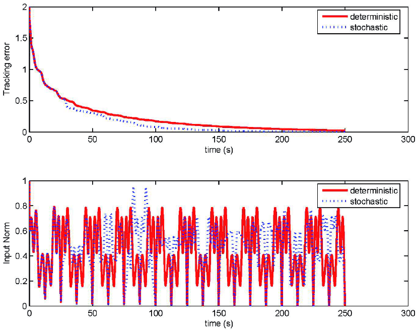
Figure 2: Convergence of the norm of the tracking error to zero and input norm. For the stochastic control law, the first choice of amplitudes $a^{j}_{k,l}$ for $j=0$ coincides with the amplitudes $a_{k,l}$ taken in deterministic control law; this explains the perfect overlaps between the solid and dotted curves for $t$ between $0$ and $T=25$.

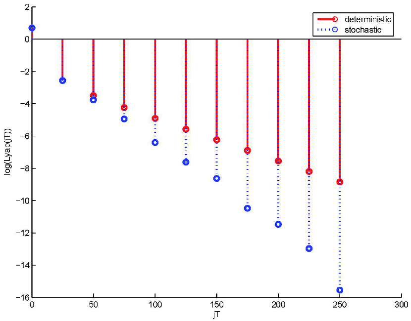
Figure 3: Logarithm of the Lyapunov function at each sampling time $t=jT$ with $T=25$.

Recall the notation $\mathbf{a}=\{a_{k,\ell}\;\in\mathbb{R}:\;k=1,\ldots,m,\;\ell=1,\ldots,M\}\in\mathbb{R}^{mM}$. To make a fair comparison, one has made a total of 50 simulations (indexed by $p$) for $t_{f}=25T=625$, for both goal matrices $X_{1_{goal}}$ and $X_{2_{goal}}$, but now with (fixed) different choices $\mathbf{a}^{p}$ of the set of amplitudes $\mathbf{a}$ for the deterministic strategy. In order to specify the $\mathbf{a}^{p}$ in the $p$-th deterministic simulation, one has chosen a random (uniformly distributed) $\mathbf{a}^{p}\in[-a_{max},a_{max}]^{mM}$. It is important to point out that the $p$-th deterministic simulation for both goal propagators uses the same fixed choice $\mathbf{a}^{p}$. The control and simulation parameters are the same as before. Figure 4 compares the obtained results. At the top, one sees the results for $X_{goal}=X_{1_{goal}}$ and, at the middle, the results for $X_{goal}=X_{2_{goal}}$. Notice that the results of the deterministic strategy depend strongly on the chosen goal matrix for a fixed $\mathbf{a}$. At the bottom of Figure 4, one sees a zoom view for $X_{goal}=X_{1_{goal}}$. Observe that the worst result of the stochastic strategy is of the order of the best result of the deterministic strategy. Simulations not shown here have indicated that, as $t_{f}/T$ gets greater, better is the performance of the stochastic strategy when compared to the deterministic one.

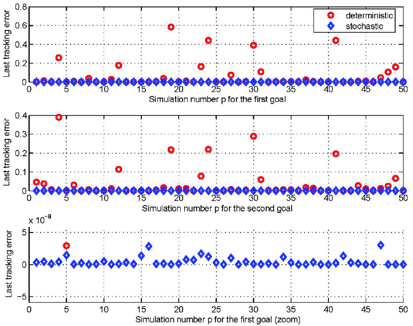
Figure 4: Error between $X$ and $X_{\mu,goal}$ at $t_{f}=25T$ for 50 Monte Carlo simulations: top corresponds to $\mu=1$, middle to $\mu=2$; bottom is a zoom for $\mu=1$.

2.4 Main Results

The next theorem shows that, for $M>0$ big enough, a random (but fixed) choice of the coefficients $a_{k,\ell},k=1,\ldots,m,\ell=1,\ldots,M$ in (5) gives a local solution to the deterministic $T$-sampling stabilization problem with probability one.

Theorem 1.

(Local Deterministic Method) Assume that (2) is controllable and that its initial condition is $X(0)=X_{0}=I$. Let $T>0$, $X_{goal}\in\mathcal{W}\subset\mbox{U}(n)$, where $\mathcal{W}$ is as in (8). Choose any nonzero $f_{1},\dots,f_{m}\in\mathbb{R}$. Fix a integer $M>0$ and a choice of $\bar{\mathbf{a}}=(\bar{a}_{k,\ell}\in\mathbb{R}\;:\;k=1,\ldots,m,\ell=1,\ldots,M)\in\mathbb{R}^{mM}$ in (5). One says that this choice of $\bar{\mathbf{a}}$ is admissible if it solves the $T$-sampling stabilization problem, that is (3) holds for the closed-loop system (7,10). Let ${\mathcal{A}}^{c}\subset\mathbb{R}^{mM}$ be the set of all non-admissible $\bar{\mathbf{a}}$. Then, there exists $M>0$ big enough such that ${\mathcal{A}}^{c}$ is closed in $\mathbb{R}^{mM}$ with zero Lebesgue measure.

The stochastic version of the result above is:

Theorem 2.

(Local Stochastic Method) Assume that (2) is controllable and that its initial condition is $X(0)=X_{0}=I$. Let $T>0$, $X_{goal}\in\mathcal{W}\subset\mbox{U}(n)$, where $\mathcal{W}$ is as in (8). Choose any nonzero $f_{1},\dots,f_{m}\in\mathbb{R}$. Fix any $a_{max}>0$. Then, there exist $\overline{M}>0$ big enough such that, for every $M\geq\overline{M}$, the stochastic control laws (15) assure that $\lim_{j\to\infty}X(jT)=X_{goal}$ almost surely.

The exponential convergence for both methods is established by:

Theorem 3.

The convergence of $X(jT)$ towards $X_{goal}$ in Theorem 1 is exponential. The almost sure convergence of $X(jT)$ towards $X_{goal}$ in Theorem 2 is also exponential.

It is important to point out that Remark 3 in Section 2.7 gives a clue of why the convergence of the stochastic method allows a greater Lyapunov exponent.

The results below solve the $T$-sampling stabilization problem for an arbitrary initial condition:

Corollary 1.

If system (2) is controllable, then the $T$-sampling stabilization problem is solvable for any initial condition $X(0)=Y_{0}\in\mbox{U}(n)$ and any goal state $Y_{goal}\in\mbox{U}(n)$ such that $Y_{goal}Y_{0}^{\dagger}\in\mathcal{W}$.

Proof.

Since (2) is a right-invariant system, one has the following well-know property. For any fixed $Z\in\mbox{U}(n)$ and any fixed set of piecewise-continuous inputs $u_{k}(t)$, $k=1,\dots,m$, then $X(t)$ is a solution of (2) if and only if $Y(t)=X(t)Z$ is a solution of (2) with the same applied inputs. Now, solve the problem for $X(0)=X_{0}=I$ and $X_{goal}=Y_{goal}Y_{0}^{\dagger}\in\mathcal{W}$ using Theorem 1 (resp. Theorem 2) and then apply the corresponding inputs (13) (resp. (15)) to system (2). Note that this corresponds to choose $Z=Y_{0}$. ∎

Remark 1.

If one accepts a global phase change on $X_{goal}$ of the form $X_{goal}\in\mbox{U}(n)\mapsto\exp(\iota\phi)X_{goal}\in\mathcal{W}\subset\mbox{U}(n)$, which is immaterial for quantum systems, then it is easy to show that, as the set of eigenvalues of $X_{goal}$ is a discrete subset of $\mathbb{C}$, one may choose a convenient $\phi$ such that Theorem 1 (deterministic) and Theorem 2 (stochastic) globally solve the $T$-sampling stabilization problem on $\mbox{U}(n)$.

It could be interesting in some situations to assure global convergence without accepting a global phase transformation. The previous result implies that one may introduce the following global strategy for the $T$-sampling stabilization of any initial state $X_{0}$ towards any goal state $X_{goal}$ that do not obey the assumption of Corollary 1.

Theorem 4.

(Global Deterministic or Stochastic Method) Given arbitrary $X_{0},X_{goal}\in\mbox{U}(n)$, then one may always construct $X_{1}\in\mbox{U}(n)$ in a way that both $X_{1}X_{0}^{\dagger}$ and $X_{goal}X_{1}^{\dagger}$ are in $\mathcal{W}$. Then one may implement the following piecewise-smooth controls law in two steps:

• Step one. Apply the control law of Corollary 1 to $Y_{0}=X_{0}$ and $Y_{goal}=X_{1}$. Then there exists $L\in\mathbb{N}$ big enough such that $X_{goal}\left.X(t)^{{\dagger}}\right|_{t=LT}=X_{goal}X(LT)^{{\dagger}}\in\mathcal{W}$.

• Step two. At the instant $\overline{t}=LT$, switch the control law to the one of Corollary 1 for $Y_{0}=X(LT)$ and $Y_{\infty}=X_{goal}$.

This control policy then solves the $T$-sampling stabilization problem.

Proof.

If $W=X_{goal}X_{0}^{\dagger}\not\in\mathcal{W}$, then one may write $W=U^{\dagger}DU$, where $U$ is a unitary matrix and $D$ is a diagonal matrix whose diagonal entries $d_{i}=\exp(\iota\theta_{i})$, $i=1,\dots,n$, are the eigenvalues of $W$. One can always assume that $\theta_{i}\in(-\pi,\pi]$, $i=1,\dots,n$. Take $W_{1}=U^{\dagger}D_{1}U$, where $D_{1}$ is a diagonal matrix with diagonal entries given by $d^{1}_{i}=\exp(\iota\theta_{i}/2),i=1,\ldots,n$. It is clear that $W=W_{1}W_{1}$ and $W_{1}\in\mathcal{W}$. Let $X_{1}=W_{1}X_{0}$. By construction, one has $X_{1}X_{0}^{\dagger}=W_{1}\in\mathcal{W}$ and $X_{goal}X_{1}^{\dagger}=WW_{1}^{\dagger}=W_{1}\in\mathcal{W}$. In the first step of our control law, one has $\lim_{j\rightarrow\infty}X(jT)=X_{1}$. By the well-known property of the continuity of eigenvalues, for $L\in\mathbb{N}$ big enough, one has $X_{goal}X(LT)^{\dagger}\in\mathcal{W}$. Then, at $\overline{t}=LT$, if one switches the control law to the one of Corollary 1 with $Y_{0}=X(LT)$ and $Y_{goal}=X_{goal}$, the claimed properties hold. ∎

2.5 Proof of the Main Deterministic Result

The technical details involved in the proof of Theorem 1 are given in the sequel.

Let $u_{k}$: $\mathbb{R}\rightarrow\mathbb{R}$, $k=1,\ldots,m$, be an arbitrary set of smooth controls and fix any initial condition $X(0)\in\mbox{U}(n)$ in (2). Define

$$\begin{array}[]{l}A(t)=\sum_{k=1}^{m}u_{k}(t)S_{k}\in\mathfrak{u}(n),\vskip 6.0pt plus 2.0pt minus 2.0pt\\ B^{0}_{k}(t)=S_{k}X(t),\vskip 6.0pt plus 2.0pt minus 2.0pt\\ B^{j+1}_{k}(t)=\dot{B}^{j}_{k}(t)-A(t)B^{j}_{k}(t),\end{array}$$ (16)

for each $j\in\mathbb{N}$, $k=1,\dots,m$, $t\in\mathbb{R}$, where $X(t)$ is the corresponding solution of (2). One remarks that the linearized system of (2) along the trajectory $(X(t),u_{k}(t),k=1\dots,m,t\in\mathbb{R})$ is given by the time-varying linear control system $\dot{X}_{\ell}(t)=A(t)X_{\ell}(t)+\sum_{k=1}^{m}w_{k}(t)B^{0}_{k}(t)$, where $X_{\ell}\in\mathbb{C}^{n\times n}$ is the state and $w_{k}\in\mathbb{R}$ are the controls [4, 6]. Let $[E,F]=EF-FE$ be the usual commutator of the matrices $E,F\in\mathbb{C}^{n\times n}$. Define

$$\begin{array}[]{rcl}C_{k}^{0}(t)&=&S_{k},\\ C_{k}^{j+1}(t)&=&\dot{C}_{k}^{j}(t)+\left[{C}_{k}^{j}(t),A(t)\right],\end{array}$$ (17)

for $k=1,\ldots m$, $j\in\mathbb{N}$, $t\in\mathbb{R}$. It is straightforward to conclude that $C^{j}_{k}(t)X(t)=B^{j}_{k}(t)$. In particular, $C^{j}_{k}(0)=B^{j}_{k}(0)$ when $X(0)=I$.

If the smooth controls $u_{k}$ are $T$-periodic and

$$u_{k}(T-t)=-u_{k}(t),\quad\mbox{for }t\in\mathbb{R},\;k=1,\dots,m,$$ (18)

then the solution $X(t)$ of (2) is also $T$-periodic (see [6] for details). It is clear that $\overline{u}_{k}$ in (5) is $T$-periodic and satisfies (18).

Definition 2.

Let $T>0$. System (2) is $T$-regular when there exist smooth $T$-periodic inputs $\widehat{u}_{k}$: $\mathbb{R}\rightarrow\mathbb{R}$, $k=1,\dots,m$, called here Coron reference controls, such that (18) holds and the corresponding $T$-periodic solution $\widehat{X}$: $\mathbb{R}\rightarrow\mbox{U}(n)$ of (2) with initial condition $\widehat{X}(0)=I$ and $u_{k}={\widehat{u}}_{k}$ satisfies

$$\mathfrak{u}(n)=\mbox{span}\{B^{j}_{k}(0),\mbox{ for all }k=1,\dots,m,\;j\in\mathbb{N}\},$$ (19)

where the $B_{k}^{j}$’s are as in (16) for the inputs $\widehat{u}_{k}$. Note that $C_{k}^{j}(0)=B_{k}^{j}(0)$ for such $\widehat{u}_{k}$. When (2) is $T$-regular for every $T>0$, one simply says that system (2) is regular.

Remark 2.

If the control problem is solved for some $T>0$, it will then be solved for all $\overline{T}>0$. This relies on standard time-scaling arguments. In fact, if $X_{a}(t)$ is a solution of (2) when the inputs are given by $u^{a}_{k}(t),k=1,\ldots,m$, then for every $\alpha>0$, one has that $X_{b}(t)=X_{a}(\alpha t)$ is a solution corresponding to the inputs $u_{k}^{b}(t)=\alpha u_{k}^{a}(\alpha t),k=1,\ldots,m$.

By redefining the Coron reference controls $\widehat{u}_{k}$ as described in Remark 2, it is clear that system (2) is regular whenever it is $T$-regular for some $T>0$. The next theorem, which relies on the results of the Return Method developed in [4], establishes that the regularity of (2) is in fact equivalent to its controllability on $\mbox{U}(n)$.

Theorem 5.

The following assertions are equivalent for system (2):

1. System (2) is regular;

2. System (2) is $T$-regular for some $T>0$;

3. $\mbox{Lie}\{S_{1},\dots,S_{m}\}=\mathfrak{u}(n)$.

Proof.

It was seen above that $1$ and $2$ are equivalent. That $2\Rightarrow 3$ follows from the presentation in [4, pp. 360, 361, 362]. Finally, $3\Rightarrow 1$ is established in [4, Remark 3.1 on p. 377] (see also [6, pp. 187–192, 296–298]). ∎

When a given set of inputs $u_{k}(t)$, $k=1,\dots,m$, are Coron reference controls, that is (19) holds and $C_{k}^{j}(0)=B_{k}^{j}(0)$, there must exist integers $k_{1},k_{2},\ldots k_{d}\in\{1,\ldots,m\}$ and $j_{1},j_{2},\ldots,j_{d}\in\mathbb{N}$ such that

$$\mathfrak{u}(n)=\mbox{span}\left\{C_{k_{h}}^{j_{h}}(0):h=1,2,\ldots,d\right\},$$ (20)

where $d\triangleq\dim\mbox{U}(n)$. However, note that the $C_{k}^{j}(0)$’s may be computed for any chosen smooth $T$-periodic controls in (2) (with initial condition $I$ at $t=0$) obeying (18), but a priori it is not assured that (20) will hold. When (20) is met, then the chosen inputs are indeed Coron reference controls.

The following theorem shows that one may generate Coron reference controls with probability one by randomly choosing the coefficients $a_{k,\ell}\in\mathbb{R}$ in (5). Note that its hypothesis is always met whenever system (2) is controllable, cf. Theorem 5.

Theorem 6.

Let $T>0$. Assume that there exists one set of Coron reference controls $\overline{u}_{k}$, $k=1,\dots,m$, for which (20) holds. Let $J=\max\{j_{1},\dots,j_{d}\}$, where $j_{h}$, $h=1,\dots,d$, are as in (20). Take $M=J/2$ (integer division). Let $\mathcal{O}\subset\mathbb{R}^{mM}$ be the set of all vectors $\bar{\mathbf{a}}=(\overline{a}_{k,\ell}\in\mathbb{R}\;:\;k=1,\ldots,m,\ell=1,\ldots,M)\in\mathbb{R}^{mM}$ for which (20) is met when $\overline{u}_{k}$, $k=1,\dots,m$, are given by (5) and $\overline{X}(t)$ is the corresponding $T$-periodic trajectory of (2) with $\overline{X}(0)=I$ and $u_{k}=\overline{u}_{k}$. Then, $\mathcal{O}$ is a dense open set in $\mathbb{R}^{mM}$ and its complement $\mathcal{O}^{c}$ has zero Lebesgue measure.

Proof.

See Appendix C. ∎

From now on, $\overline{u}_{k}$, $k=1,\dots,m$, will denote a choice of Coron reference controls and $\overline{X}_{I}(t)$ will be the corresponding $T$-periodic trajectory of (2) with $\overline{X}_{I}(0)=I$ and $u_{k}=\overline{u}_{k}$. Given any desired goal state $X_{goal}\in\mbox{U}(n)$, define

$$\overline{X}(t)=\overline{X}_{I}(t)X_{goal},\quad t\in\mathbb{R}.$$ (21)

Note that $\overline{X}(t)$ is the resulting $T$-periodic reference trajectory of (6) with $\overline{X}(0)=X_{goal}$ and the same controls. Our main stability result is now presented.

Theorem 7.

Choose $T>0$. Let $X_{0}=X(0)=I$ and $X_{goal}\in\mathcal{W}$. Let $\overline{u}_{k},k=1,\ldots,m$, be Coron reference controls and let $\overline{X}(t)$ be the $T$-periodic reference trajectory of (6) given in (21). Then the control laws $\widetilde{u}_{k}$ in (10) solve the $T$-sampling stabilization problem, that is (3) holds for the closed-loop system (7,10).

Proof.

The idea of the proof is the application of Lasalle’s invariance principle, Theorem 8 in Appendix B. For this, consider the closed-loop system (7,10) with state evolving on $S=\{\tilde{X}\in\mathbb{C}^{n\times n}\;|\;\det(I+X)\neq 0\}$. In this case, one is regarding a system evolving on an open set of a (complex) Euclidean space. Recall that the set $K\subset\mathcal{W}\subset S$ defined by (12) is a compact positively invariant set.

Then, for any $\widetilde{X}(0)=\widehat{X}\in K$, the solution $\widetilde{X}(t)$ of (7,10) is defined for all $t\geq 0$ and remains inside $K$. Since (7,10) is a $T$-periodic system, then by Theorem 8 it suffices to show that the set

$$E=\{(\widehat{X},t)\in K\times\mathbb{R}^{+}\;|\;\dot{\mathcal{V}}(\widehat{X},t)=0\}$$

does not contain any nontrivial solution $(\widetilde{X}(t),t)$, $t\geq 0$, of (7,10), that is only the trivial solution $(I,t)$, $t\geq 0$ is contained in $E$. For that, according to (11), $\dot{\mathcal{V}}(\widetilde{X}(t),t)=0$ for all $t\geq 0$ along a solution implies that the control law (10) is identically zero. Hence, such a solution must be an equilibrium point of (7), that is $\widetilde{X}(t)$ must identically equal to its initial condition $\widetilde{X}(0)=\widehat{X}$. Now, in (11), let

$$\widehat{Z}=\widehat{X}(\widehat{X}-I)(\widehat{X}+I)^{-3}.$$ (22)

Suppose that $\mbox{Tr}\left(\widehat{Z}\overline{X}^{{\dagger}}(t)S_{k}\overline{X}(t)\right)=\mbox{Tr}\left(\widehat{Z}\overline{X}^{{\dagger}}(t)C_{k}^{0}(t)\overline{X}(t)\right)=0$ for $t\in[0,T]$, $k=1,\ldots,m$. It will be shown by induction that, for $k=1,\ldots,m$, one has

$$\mbox{Tr}\left(\widehat{Z}\overline{X}^{{\dagger}}(t)C_{k}^{j}(t)\overline{X}(t)\right)=0,\quad\mbox{for }t\in[0,T],\;j\in\mathbb{N}.$$ (23)

This is true for $j=0$ and assume it holds for a fixed $j\in\mathbb{N}$. Taking the derivative at both sides of (23) and using (17), one obtains

$$\begin{array}[]{l}\mbox{Tr}\left(\widehat{Z}\left[\dot{\overline{X}}^{{\dagger}}(t)C_{k}^{j}(t)\overline{X}(t)\right]\right)+\mbox{Tr}\left(\widehat{Z}\left[\overline{X}^{{\dagger}}(t)\dot{C}_{k}^{j}(t)\overline{X}(t)\right]\right)+\mbox{Tr}\left(\widehat{Z}\left[\overline{X}^{{\dagger}}(t)C_{k}^{j}(t)\dot{\overline{X}}(t)\right]\right)\\ =\mbox{Tr}\left(\widehat{Z}\left(\overline{X}^{{\dagger}}(t)\dot{C}_{k}^{j}(t)\overline{X}(t)\ \right)\right)+\mbox{Tr}\left(\widehat{Z}\left(\overline{X}^{{\dagger}}(t)\left[C_{k}^{j}(t),\sum_{\ell=1}^{m}u_{\ell}^{T}(t)S_{\ell}\right]\overline{X}(t)\right)\right)\\ =\mbox{Tr}\left(\widehat{Z}\overline{X}^{{\dagger}}(t)C_{k}^{j+1}(t)\overline{X}(t)\right)=0,\quad\mbox{for }t\in[0,T].\end{array}$$

Hence (23) holds. Taking $t=0$, one gets

$$\mbox{Tr}\left(\widehat{Z}\overline{X}(0)^{{\dagger}}C_{k}^{j}(0)\overline{X}(0)\right)=\mbox{Tr}\left(\widehat{Z}X_{goal}^{{\dagger}}C_{k}^{j}(0)X_{goal}\right)=0.$$

By (19) and from the fact that $C_{k}^{j}(0)$=$B_{k}^{j}(0)$, to conclude the proof it suffices to show that $\mbox{Tr}\left(\widehat{Z}\Sigma\right)=0$, for $\widehat{Z}$ given by (22) and all $\Sigma\in\mathfrak{u}(n)$, implies that $\widehat{X}=I$. Recall that one may write $\widehat{X}=U^{\dagger}DU$, where $U$ is unitary, $D=\text{diag}(\exp{(\iota a_{1})},\ldots,\exp{(\iota a_{n})})$ is a diagonal matrix, and $d_{i}=\exp{(\iota a_{i})},i=1,\ldots,n$, are the eigenvalues of $\widehat{X}$ with $a_{i}\in(-\pi,\pi)$. Note that $\det\widehat{X}=1$ implies that $\sum_{i=1}^{n}a_{i}=0$ (mod $2\pi$). Simple computations using the identities $\exp{(\iota a)}-1=2\iota\sin(a/2)\exp{(\iota a/2)}$ and $\exp{(\iota a)}+1=2\cos(a/2)\exp{(\iota a/2)}$ results in $\widehat{Z}=U^{{\dagger}}D_{1}U$, where $D_{1}=\text{diag}(\iota\alpha(a_{1}),\ldots,\iota\alpha(a_{n}))$ with $\alpha(a_{i})=\tan(a_{i}/2)/[2\cos(a_{i}/2)]^{2}$. It is easy to show that the function $(-\pi,\pi)\ni a\mapsto\alpha(a)=\tan(a/2)/[2\cos(a/2)]^{2}\in\mathbb{R}$ is injective, it is surjective (onto $\mathbb{R}$), and $\alpha(0)=0$. Now, taking the matrices in $\mathfrak{u}(n)$ of the form $U^{{\dagger}}\Xi U$ with

$$\Xi=\text{diag}(0,\ldots,0,0,\ldots,0,-\iota,0,\ldots,0)\in\mathfrak{u}(n)$$ (24)

and using the invariance of the trace, one obtains that all the diagonal entries of $D_{1}$ are zero. As the map $\alpha$ is injective, it follows that $a_{i}=0,i=1,\ldots,n$, and this concludes the proof. ∎

Proof.

(of Theorem 1) A straightforward consequence of Theorem 5, Theorem 6 and Theorem 7. ∎

2.6 Proof of the Main Stochastic Result

This subsection presents the proof of Theorem 2. First of all, the tracking error $\widetilde{X}(t)$ is sampled with sampling period $T$ in order to apply stochastic Lyapunov stability results that will assure that $\lim_{j\to\infty}\widetilde{X}(jT)=I$. Now, for each sampling interval $[jT,(j+1)T)$, $j\in\mathbb{N}$:

• One considers the reference controls as in (14);

• One defines similarly the reference trajectory $\overline{X}(t)$, the tracking error $\widetilde{X}(t)$ and the feedbacks $\widetilde{u}_{k}(t)$ by taking $\overline{u}_{k}(t)$ as in (14);

• One lets $\widetilde{X}_{j}=\widetilde{X}(jT)\in\mathcal{W}$ for $j\in\mathbb{N}$.

The vector field of the closed-loop system (7,10) with the choice (5) depends smoothly on the reference controls parameters $a_{k,\ell}$. Recall that $\widetilde{S}_{k}(t)=\overline{X}^{{\dagger}}(t)S_{k}\overline{X}(t)$, where the reference trajectory $\overline{X}(t)$ is the solution of (6) with the reference controls $\overline{u}_{k}(t)$ in (5). Let $\Lambda$: $\mathbb{R}\times\mathbb{R}\times\mathcal{W}\times\mathbb{R}^{mM}\rightarrow\mathcal{W}$ be the ($\mathbf{a}$-parameter dependent) smooth global flow of the closed-loop system (5,7,10). This means that $\widetilde{X}(t)=\Lambda(t,t_{0},\widehat{X},\mathbf{a})\in\mathcal{W}$, is the solution of system (7,10) with the choice (5) and with initial condition $\widetilde{X}(t_{0})=\widehat{X}\in\mathcal{W}$ at $t=t_{0}$ and reference controls parameters $\mathbf{a}=(a_{k,\ell})\in\mathbb{R}^{mM}$. In particular, the map $(\widetilde{X},\mathbf{a})\ni\mathcal{W}\times\mathbf{A}\mapsto\Lambda(T,0,\widetilde{X},\mathbf{a})\in\mathcal{W}$ is continuous. Since system (5,7,10) is $T$-periodic in $t$, one has that $\Lambda(t+jT,jT,\widetilde{X},\mathbf{a})=\Lambda(t,0,\widetilde{X},\mathbf{a})$ for every $t\geq 0$, $j\in\mathbb{N}$, $(\widetilde{X},\mathbf{a})\in\mathcal{W}\times\mathbf{A}$ [25, p. 143].

The reasoning above implies that $\widetilde{X}_{j+1}=\Lambda(T,0,\widetilde{X}_{j},\mathbf{a}_{j})$, for $j\in\mathbb{N}$, where $\widetilde{X}_{0}=X_{goal}\in\mathcal{W}$. Consequently, $\widetilde{X}_{j}$: $\mathbb{N}\rightarrow\mathcal{W}$ is a Markov chain (with respect to the natural filtration and the Borel algebra on $\mathcal{W}$) because $\mathbf{a}_{j}$, $j\in\mathbb{N}$, are independent random vectors. Note that (11) assures that $\mathcal{V}(\widetilde{X}_{j})$, $j\in\mathbb{N}$, is a supermartingale. Define the continuous function $Q$: $\mathcal{W}\rightarrow\mathbb{R}$ as

$$Q(\widehat{X}) \triangleq\frac{-1}{a_{max}^{mM}}\int_{\mathbf{A}}\left(\int_{0}^{T}\dot{\mathcal{V}}\left(\Lambda(t,0,\widehat{X},\mathbf{a}),t\right)\,dt\right)\,d\mathbf{a}=\frac{-1}{a_{max}^{mM}}\int_{\mathbf{A}}\left(\int_{0}^{T}\dot{\mathcal{V}}\left(\widetilde{X}(t),t\right)\,dt\right)\,d\mathbf{a}.$$ (25)

By (11), $Q$ is non-negative, and (10) gives that $Q(I)=0$. For each $j\in\mathbb{N}$, the conditional expectation of $\mathcal{V}(\widetilde{X}_{j+1})$ knowing $\widetilde{X}_{j}$ is denoted by $\mathbb{E}\left(\mathcal{V}(\widetilde{X}_{j+1})/\widetilde{X}_{j}\right)$. Since $\widetilde{X}_{j}$ is independent of $\mathbf{a}_{j}$ and $\dot{\mathcal{V}}(\widetilde{X},t)$ is $T$-periodic in $t$, one gets

$$\mathbb{E}\left(\mathcal{V}(\widetilde{X}_{j+1})/\widetilde{X}_{j}\right)-\mathcal{V}(\widetilde{X}_{j})=\frac{1}{a_{max}^{mM}}\left.\left[\int_{\mathbf{A}}\left(\int_{jT}^{(j+1)T}\dot{\mathcal{V}}\left(\Lambda(t,jT,\widehat{X},\mathbf{a}),t\right)\,dt\right)d\mathbf{a}\right]\right|_{\widehat{X}=\widetilde{X}_{j}}=-Q(\widetilde{X}_{j}).$$ (26)

Standard results on stochastic Lyapunov stability imply that $\lim_{j\to\infty}Q(\widetilde{X}_{j})=0$ almost surely (see Theorem 9 in Appendix). One will show that the only solution to $Q(\widehat{X})=0$ is $\widehat{X}=I$. This will prove almost sure convergence of $\widetilde{X}_{j}=\widetilde{X}(jT)$ towards $I$ because $Q$ is continuous and $\widetilde{X}_{j}$ evolves on the compact set $K=\{\widetilde{X}\in\mathcal{W}\;|\;0\leq\mathcal{V}(\widetilde{X})\leq\mathcal{V}(X_{goal})\}$ in $\mathcal{W}$.

Assume that $\widehat{X}\in\mathcal{W}$ is such that $Q(\widehat{X})=0$. Then, $\dot{\mathcal{V}}(\Lambda(t,0,\widehat{X},\mathbf{a}),t)=0$ for $t\in[0,T]$ and $\mathbf{a}=(a_{k,\ell})\in\mathbf{A}$. In particular, (11) implies that $\widetilde{u}_{k}(t)=0$ for $t\in[0,T)$. By relying on the ideas presented in the end of the proof Theorem 7, one concludes that $\widetilde{X}=I$. The preceding argument then proves that $\lim_{j\to\infty}\widetilde{X}(jT)=I$ almost surely, which completes the proof of Theorem 2.

2.7 Proof of the Exponential Convergence Result

Theorem 3 for the deterministic strategy is immediate from the result given below and standard Lyapunov stability results for discrete-time nonlinear systems.

Lemma 1.

Let $\|\widetilde{W}\|=\mbox{Tr}(\widetilde{W}^{\dagger}\widetilde{W})$ stand for the Frobenius norm of $\widetilde{W}\in\mathbb{C}^{n\times n}$. Then:

• There exist $\epsilon_{1},c_{1},c_{2}>0$ such that, for every $\widetilde{X}\in\mbox{U}(n)$ with $\|\widetilde{X}-I\|<\epsilon_{1}$, then

  $$c_{1}\|\widetilde{X}-I\|^{2}\leq\mathcal{V}(\widetilde{X})\leq c_{2}\|\widetilde{X}-I\|^{2}.$$ (27)

• There exist $\epsilon_{2},c_{3},c_{4}>0$ such that, for every $\widetilde{X}\in\mbox{U}(n)$ with $\|\widetilde{X}-I\|<\epsilon_{2}$, then

  $$c_{3}\|\widetilde{X}-I\|^{2}\leq\|Z\|^{2}\leq c_{4}\|\widetilde{X}-I\|^{2},\quad\mbox{where }Z=\widetilde{X}(\widetilde{X}-1)(\widetilde{X}+I)^{-3}.$$ (28)

• If $\mathbf{a}\in\mathbf{A}$ is admissible in the sense of Theorem 1, then there exists $M_{\mathbf{a}}>0$ such that, for the trajectory $\widetilde{X}(t)$ of the closed-loop system (7,10) with initial condition $\widetilde{X}(0)=X_{goal}\in\mathcal{W}$, there exists $L\in\mathbb{N}$ big enough such that, for all $j\geq L$, one has

  $${\mathcal{V}}(\widetilde{X}((j+1)T))-{\mathcal{V}}(\widetilde{X}(jT))\leq-M_{\mathbf{a}}\|\widetilde{X}(jT)-I\|^{2}.$$ (29)

Proof.

The first claim is an immediate consequence of (41) (see Appendix A), and the second one is straightforward from the properties of the function $\alpha$ used in the proof of Theorem 7. Consider now that $X_{goal}$ is such that $\|X_{goal}-I\|\leq\min\{\epsilon_{1},\epsilon_{2}\}$. Then the proof of the third claim follows from the arguments below:

• Let $\mathbf{G}$ be the set of skew-Hermitian matrices of unitary (Frobenius) norm. It is clear that $\mathbf{G}$ is compact. By using similar arguments as in the end of the proof of Theorem 7, it is easy to show that, for any fixed $Z^{*}\in\mathbf{G}$, one has

  $$\int_{0}^{T}\sum_{k=1}^{m}f_{k}\mbox{Tr}^{2}(Z^{*}\widetilde{S}_{k}(t))\,dt\triangleq P_{\mathbf{a}}(Z^{*})>0.$$

• As $P_{\mathbf{a}}(\cdot)$ is continuous in $Z^{*}\in\mathbf{G}$ and $\mathbf{G}$ is compact, this function admits a minimum $P_{\mathbf{a}}^{*}>0$. Thus, for any fixed $Z^{*}\in\mathbf{G}$,

  $$\int_{0}^{T}\sum_{k=1}^{m}f_{k}\mbox{Tr}^{2}(Z^{*}\widetilde{S}_{k}(t))\,dt\geq P_{\mathbf{a}}^{*}>0.$$ (30)

• Fix $X_{goal}\in\mathcal{W}$ and let $K$ be the set in (12). Recall that $K$ is positively invariant and compact, cf. Appendix A. Consider the continuous map $K\ni\widetilde{X}\mapsto Z(\widetilde{X})=\widetilde{X}(\widetilde{X}-I)(\widetilde{X}+I)^{-3}\in\mathbb{C}^{n\times n}$. Let $Z(t)=Z(\widetilde{X}(t))=\widetilde{X}(t)(\widetilde{X}(t)-I)(\widetilde{X}(t)+I)^{-3}$, for $t\geq 0$, where $X(t)\in K$ is the solution of the closed-loop system (7,10) with initial condition $\widetilde{X}(0)\in K-\{I\}$. From the same arguments of the end of the proof of Theorem 7 (see the relationship between $\widehat{Z}$ and $\widetilde{X}$), one concludes that $Z_{0}=Z(0)\neq 0$ and $Z_{0}/\|Z_{0}\|\in\mathbf{G}$. By uniqueness of solutions, $Z(0)\neq 0$ implies that $Z(t)\neq 0$ for $t\in[0,T]$.

• It will be shown by contradiction that there exists $N_{\mathbf{a}}>0$ such that, for all $\widetilde{X}(0)\in K-\{I\}$, one has

  $$\int_{0}^{T}\sum_{k=1}^{m}f_{k}\mbox{Tr}^{2}(Z(t)\widetilde{S}_{k}(t))\,dt\geq N_{\mathbf{a}}\|Z_{0}\|^{2}.$$ (31)

  Assume that this is not the case. Hence, for every $n\in\mathbb{N}$ with $n>0$, there exists $\widetilde{X}_{n}(0)\in K-\{I\}$ such that

  $$\int_{0}^{T}\sum_{k=1}^{m}f_{k}\mbox{Tr}^{2}(Z_{n}(t)\widetilde{S}_{k}(t))\,dt=\int_{0}^{T}\sum_{k=1}^{m}\left(\frac{\widetilde{u}_{k,n}(t)}{\sqrt{f_{k}}}\right)^{2}\,dt<\dfrac{1}{n}\|Z_{0n}\|^{2},$$ (32)

  where $Z_{0n}=Z_{n}(0)$ and $\widetilde{u}_{k,n}(t)=\widetilde{u}_{k,n}(\widetilde{X}_{n}(t),t)$ is as in (10). Fix $n\in\mathbb{N}$ with $n>0$. The Cauchy-Schwartz inequality provides that (see (46) of Appendix (D)), for $t\in[0,T]$,

  $$\int_{0}^{t}\left|\frac{\widetilde{u}_{k,n}(s)}{\sqrt{f_{k}}}\right|\,ds\leq\int_{0}^{T}\left|\frac{\widetilde{u}_{k,n}(s)}{\sqrt{f_{k}}}\right|\,ds\leq\sqrt{T}\sqrt{\int_{0}^{T}\left(\frac{\widetilde{u}_{k,n}(t)}{\sqrt{f_{k}}}\right)^{2}\,dt}<\sqrt{T/n}\|Z_{0n}\|.$$ (33)

  Now, using the fact that $X_{n}(t)\in K$, standard computations show that

  $$\dot{Z}_{n}(t)=\sum_{k=1}R_{k}(X_{n}(t))\widetilde{u}_{k,n}(t),$$

  where $R_{k}(t)=R_{k}(X_{n}(t))$ is continuous and uniformly bounded on $[0,T]$ by some $D_{k}>0$. Thus, for every $t\in[0,T]$,

  $$\left\|\dfrac{Z_{n}(t)-Z_{0n}}{\|Z_{0n}\|}\right\|=\left\|\int_{0}^{t}\dfrac{\dot{Z}_{n}(s)}{\|Z_{n0}\|}\,ds\right\|\leq\sum_{k=1}^{m}D_{k}\int_{0}^{t}\frac{|\widetilde{u}_{k,n}(s)|}{\|Z_{0n}\|}\,ds.$$ (34)

  From (33) and (34), it follows that

  $$\left\|\dfrac{Z_{n}(t)-Z_{0n}}{\|Z_{0n}\|}\right\|\leq fD\sqrt{T/n},$$

  where $D=D_{1}+\dots+D_{m}>0$ and $f=\max\{\sqrt{f_{1}},\dots,\sqrt{f_{m}}\}>0$. As the sequence $Z_{0n}/\|Z_{0n}\|$ belongs to the compact set $\mathbf{G}$, there exists a convergent subsequence. For simplicity, denote such subsequence by $Z_{0n}/\|Z_{0n}\|$ and let $Z^{*}\in\mathbf{G}$ be its limit. It follows that $Z_{n}(t)/\|Z_{0n}\|$ uniformly converges to $Z^{*}$ on the interval $[0,T]$ as $n\to\infty$. Consequently, (30) gives that

  $$\lim_{n\to\infty}\int_{0}^{T}\sum_{k=1}^{m}\mbox{Tr}^{2}\left(\dfrac{Z_{n}(t)}{\|Z_{n0}\|}\widetilde{S}_{k}(t)\right)\,dt=\int_{0}^{T}\sum_{k=1}^{m}\mbox{Tr}^{2}(Z^{*}\widetilde{S}_{k}(t))\,dt\geq P_{\mathbf{a}}^{*}>0.$$

  However, (32) and the fact that $\mbox{Tr}^{2}\left(\dfrac{Z_{n}(t)}{\|Z_{n0}\|}\widetilde{S}_{k}(t)\right)=\dfrac{1}{\|Z_{n0}\|^{2}}\mbox{Tr}^{2}\left(Z_{n}(t)\widetilde{S}_{k}(t)\right)$ implies that the limit above is zero, which is a contradiction.

• Using (11), (28) and (31), one obtains

  $$\mathcal{V}(\widetilde{X}((j+1)T))-\mathcal{V}(\widetilde{X}(jT)) =\int_{jT}^{(j+1)T}-4\sum_{k=1}^{m}f_{k}\mbox{Tr}^{2}({Z(t)}\widetilde{S}_{k}(t))\,dt$$

  $$\leq-4N_{\mathbf{a}}\|Z(jT)\|^{2}\leq-4c_{3}N_{\mathbf{a}}\|\widetilde{X}(jT)-I\|^{2}.$$

• The results above considered a fixed $X_{goal}$ and the associated compact set $K$. Now, since $\mathcal{V}(I)=0$, and by Theorem 1 one has $\lim_{t\to\infty}\widetilde{X}(t)=I$ for any given initial condition $\widetilde{X}(0)=\overline{X}_{goal}\in\mathcal{W}$ of the closed-loop system, it is clear that there always exists $\overline{t}\geq 0$ such that $\widetilde{X}(\overline{t})\in K$.

∎

The proof of Theorem 3 for the stochastic strategy has a similar structure, and is now presented.

Proof.

In this proof one will denote by $\widetilde{X}^{\mathbf{a}}(t)$ the solution of the closed loop system (7,10) with initial condition $\widetilde{X}(0)=X_{0}$, where $\mathbf{a}$ is the set of amplitudes $a_{k,\ell},k=1,\ldots,M,\ell=1,\ldots,M$, defining the reference control (5). Then $Z^{\mathbf{a}}(t)$ is a skew-Hermitean matrix given by $Z^{\mathbf{a}}(t)=\widetilde{X}^{\mathbf{a}}(t)(\widetilde{X}^{\mathbf{a}}(t)-I)(\widetilde{X}^{\mathbf{a}}(t)+I)^{-3}$. Note that if $X_{0}\in K$, where $K$ is the positively invariant compact set defined by (12), then $Z^{\mathbf{a}}(t)$ is uniformly bounded on $\mathbf{A}\times[0,\infty)$. Furthermore, as in the deterministic strategy, by uniqueness of solutions, if $\widetilde{X}_{0}=\widetilde{X}(0)\neq I$, it is clear that $\widetilde{X}^{\mathbf{a}}(t)\neq I$ and $Z^{\mathbf{a}}(t)\neq 0$ for all $t\geq 0$. Let $Z_{0}=Z^{\mathbf{a}}(0)$.

According to [12, Theorem 2(8.8c), p. 197] and from properties (27) and (28) of Lemma 1, it suffices to show that there exists $M>0$ such that $Q(\widetilde{X}_{0})\geq M\|Z_{0}\|^{2}$, for all $\widetilde{X}_{0}\in K$, where $Q$ is defined by (25). Assume the contrary. Then, from (10) and (11), one has that for all $n\in\mathbb{N}$ with $n>0$, there exists $\widetilde{X}_{0n}\in K-\{I\}$ such that

$$\int_{\mathbf{A}}\left[\int_{0}^{T}\sum_{k=1}^{m}f_{k}\mbox{Tr}^{2}\left(Z^{\mathbf{a}}_{n}(t)\widetilde{S}^{\mathbf{a}}_{k}(t)\right)dt\right]d\mathbf{a}=\int_{\mathbf{A}}\int_{0}^{T}\left[\sum_{k=1}^{m}\left(\frac{\widetilde{u}_{k,n}^{\mathbf{a}}(t)}{\sqrt{f_{k}}}\right)^{2}dt\right]d\mathbf{a}<\frac{1}{n}\|Z_{0n}\|^{2}.$$ (35)

Using (35), the Cauchy-Scharwz inequality (see (46) in Appendix D), and the fact that $\mbox{vol}\left(\mathbf{A}\times[0,T]\right)=\mbox{vol}\left(\mathbf{A}\right)T$ (Lebesgue measure), one obtains:

$$\int_{\mathbf{A}}\int_{0}^{t}\left|\left(\frac{\widetilde{u}_{k,n}^{\mathbf{a}}(t)}{\sqrt{f_{k}}}\right)\right|dt\,d\mathbf{a}\leq\int_{\mathbf{A}}\int_{0}^{T}\left|\left(\frac{\widetilde{u}_{k,n}^{\mathbf{a}}(t)}{\sqrt{f_{k}}}\right)\right|dt\,d\mathbf{a}\leq\sqrt{\mbox{vol}(\mathbf{A})T/n}\|Z_{0n}\|,\quad t\in[0,T].$$ (36)

Now, by the same reasoning that was used to obtain (34), one may write

$$\int_{\mathbf{A}}\left\|\dfrac{Z^{\mathbf{a}}_{n}(t)-Z_{0n}}{\|Z_{0n}\|}\right\|d{\mathbf{a}}=\left\|\int_{\mathbf{A}}\int_{0}^{t}\dfrac{\dot{Z}_{n}^{\mathbf{a}}(s)}{\|Z_{n0}\|}\,ds\,d{\mathbf{a}}\right\|\leq\int_{\mathbf{A}}\sum_{k=1}^{m}D_{k}\int_{0}^{t}\frac{\left|\widetilde{u}_{k,n}^{\mathbf{a}}(s)\right|}{\|Z_{0n}\|}\,ds\,d{\mathbf{a}},\quad t\in[0,T],$$ (37)

where $D_{k}>0$, and so by (36) and (37) it follows that

$$\int_{\mathbf{A}}\left\|\dfrac{Z^{\mathbf{a}}_{n}(t)-Z_{0n}}{\|Z_{0n}\|}\right\|d{\mathbf{a}}\leq fD\sqrt{\mbox{vol}(A)T/n},\quad t\in[0,T],$$

where $D=D_{1}+D_{2}+\ldots+D_{m}>0$ and $f=\max\{\sqrt{f_{1}},\ldots,\sqrt{f_{m}}\}>0$. From this last equation, one gets

$$\int_{\mathbf{A}}\int_{0}^{T}\left\|\dfrac{Z^{\mathbf{a}}_{n}(t)-Z_{0n}}{\|Z_{0n}\|}\right\|dt\,d{\mathbf{a}}\leq TfD\sqrt{\mbox{vol}(A)T/n}.$$ (38)

Up to a convenient subsequence, one may assume that the sequence $\frac{Z_{0n}}{\|Z_{0n}\|}$ converges to some $Z^{*}\in\mathbf{G}$. Then (38) implies that $\frac{Z^{\mathbf{a}}_{n}(t)}{\|Z_{0n}\|}$ converges to $Z^{*}$ in the $L^{1}$ sense:

$$\lim_{n\to\infty}\int_{\mathbf{A}}\int_{0}^{T}\left\|\dfrac{Z^{\mathbf{a}}_{n}(t)}{\|Z_{0n}\|}-Z^{*}\right\|dt\,d{\mathbf{a}}=0.$$ (39)

Note that the sequence $Z^{\mathbf{a}}_{n}(t)$ is uniformly bounded on $\mathbf{A}\times[0,T]$ and that (35) implies that

$$\int_{\mathbf{A}}\left[\int_{0}^{T}\sum_{k=1}^{m}f_{k}\mbox{Tr}^{2}\left(\frac{Z^{\mathbf{a}}_{n}(t)}{\|Z_{0n}\|}\widetilde{S}_{k}^{\mathbf{a}}(t)\right)dt\right]d\mathbf{a}<\frac{1}{n}.$$ (40)

Furthermore, note that $\mbox{Tr}^{2}\left(\frac{Z^{\mathbf{a}}_{n}(t)}{\|Z_{0n}\|}\widetilde{S}_{k}(t)\right)$ is a sum of products of the form $z_{ij}\,z_{kl}\,\widetilde{s}_{pq}\,\widetilde{s}_{rs}$, where $z_{ij}$ denotes an element of $\dfrac{Z^{\mathbf{a}}_{n}(t)}{\|Z_{0n}\|}$ and $\widetilde{s}_{pq}$ denotes an element of $\widetilde{S}_{k}^{\mathbf{a}}(t)$. From Lemma 2 of Appendix D, it follows that, by taking the limit $n\rightarrow\infty$, one may replace $\dfrac{Z^{\mathbf{a}}_{n}(t)}{\|Z_{0n}\|}$ by its limit $Z^{*}\in\mathbf{G}$ in the integral (40):

$$\lim_{n\rightarrow\infty}\int_{\mathbf{A}}\int_{0}^{T}\sum_{k=1}^{m}f_{k}\mbox{Tr}^{2}\left(\frac{Z^{\mathbf{a}}_{n}(t)}{\|Z_{0n}\|}\widetilde{S}_{k}^{\mathbf{a}}(t)\right)dt\,d\mathbf{a}=\int_{\mathbf{A}}\int_{0}^{T}\sum_{k=1}^{m}f_{k}\mbox{Tr}^{2}\left(Z^{*}\widetilde{S}_{k}^{\mathbf{a}}(t)\right)dt\,d\mathbf{a}.$$

Now note that, for a fixed $Z^{*}\in\mathbf{G}$, then (30) holds for almost all $\mathbf{a}\in\mathbf{A}$ (cf. Theorem 1). The continuous dependence of the $T$-periodic reference trajectory $\overline{X}(t)$ with respect to the set of parameters ${\mathbf{a}}$ implies that the $T$-periodic map $\widetilde{S}^{\mathbf{a}}_{k}(t)$ also depends continuously on $\mathbf{a}$, and hence

$$\lim_{n\rightarrow\infty}\int_{\mathbf{A}}\int_{0}^{T}\sum_{k=1}^{m}f_{k}\mbox{Tr}^{2}\left(\frac{Z^{\mathbf{a}}_{n}(t)}{\|Z_{0n}\|}\widetilde{S}_{k}^{\mathbf{a}}(t)\right)dt\;d\mathbf{a}>0.$$

However, (40) implies that the same limit is zero, which is a contradiction. ∎

Remark 3.

The last proof and (28) imply that $Q({\widetilde{X}_{0}})\geq M\|{\widetilde{X}_{0}}-I\|^{2}$. Note that this does not explain why the convergence of the stochastic method is faster. The authors believe that this is due to the following fact. Consider a realization of the stochastic method such that (29) holds in each step of both deterministic and stochastic methods. Note that $M_{\mathbf{a}}$ regards the worst direction, that is, for some ${\widetilde{X}}_{0}={\widetilde{X}}_{0}^{\mathbf{a}}$ one has that $V({\widetilde{X}}_{f})-V({\widetilde{X}}_{0})$ is of order $M_{\mathbf{a}}\|{\widetilde{X}}_{0}-I\|^{2}$. It seems that the “worst direction” ${\widetilde{X}}_{0}^{\mathbf{a}}$ is very sensible to $\mathbf{a}$, assuring that the next aleatory steps will provide a compensation of the speed just by varying the worst direction, and then providing a better speed in an average process.

3 Concluding Remarks

In this work one has proposed a constructive solution of the $T$-sampling stabilization problem for quantum systems on $\mbox{U}(n)$. It is easy to show that the complement $\mathcal{W}^{c}$ of the set $\mathcal{W}$ in (8) is closed with Lebesgue measure zero, and $\mathcal{W}$ is dense in $\mbox{U}(n)$. It was also shown that, if one accepts a global phase change on $X_{goal}$ of the form $X_{goal}\in\mbox{U}(n)\mapsto\exp(\iota\phi)X_{goal}\in\mathcal{W}\subset\mbox{U}(n)$, which is transparent for quantum systems, one may always obtain an equivalent $X_{goal}$ inside $\mathcal{W}$. From this perspective, the two steps procedure of Theorem 4 for $T$-sampling stabilization may be completely avoided. However, note from (10) that the feedbacks $\widetilde{u}_{k}$ tends to infinity when the initial condition $\widetilde{X}(0)$ tends to $\mathcal{W}^{c}$. For initial conditions that are close to $\mathcal{W}^{c}$, simulations have shown a better compromise of the convergence speed versus the maximum norm of the input when one chooses the two-step procedure instead of the single one.

The approach of this paper is based on previous results of [20, 21] which provided a solution of the $T$-sampling stabilization problem for controllable systems (2) on $\mbox{SU}(n)$ in a certain number of steps that may grow with $n$. In the present work, a new Lyapunov function $\mathcal{V}$ is defined. This new choice assures a complete and global solution of the problem when the system is controllable, since $\mathcal{V}$ essentially decreases without singularities and with no nontrivial LaSalle’s invariants. The results of [20] are based on the existence of a special kind of $T$-periodic reference trajectory which is generated by special inputs, called here Coron reference controls, in a way that the linearized system is controllable along such trajectory. In [20] it is not shown how to construct a trajectory with such properties, and in [21] it is indeed constructed when the system obeys the $p$-controllability condition. This paper relaxed such condition by assuming only that the system is controllable. Another important contribution of this work was to show that, for a number of frequencies $M>0$ big enough, the inputs of the form $\overline{u}_{k}(t)=\sum_{\ell=1}^{M}a_{k,\ell}\sin(2\pi t/T)$ generate Coron reference controls with probability one with respect to a random choice of the real coefficients $a_{k,\ell}$. This result implies that the control laws required in the present work and in [20] are completely constructible. Furthermore, one has established that the convergence of the $T$-sampling stabilization problem is exponential for both methods, deterministic an stochastic. It is important to point out that the speed of exponential convergence may be controlled if one chooses $\overline{T}=T/c$, $\overline{f}_{k}=cf_{k}$, $\overline{\mathbf{a}}=c\mathbf{a}$, where $c>0$. This is immediate from Remark 2.

The methods presented here could be adapted to controllable quantum models (2) that evolve on the special unitary group $\mbox{SU}(n)$ as well, but this will be the subject of a future work.

Appendix A Compactness of $K$

Proposition 1.

The set $K$ in (12) is compact in $\mathcal{W}$.

Proof.

As $\mbox{U}(n)$ is compact, it suffices to show that $K$ is closed in $\mbox{U}(n)$. For this, assume that $W_{k}\in K$ is a sequence with $\lim_{k\rightarrow\infty}W_{k}=\overline{W}\in\mbox{U}(n)$. If $\overline{W}\in\mathcal{W}$, then the continuity of $\mathcal{V}$ in $\mathcal{W}$ gives $\lim_{k\rightarrow\infty}\mathcal{V}(X_{k})=\mathcal{V}(\lim_{k\rightarrow\infty}X_{k})=\mathcal{V}(\overline{W})$. As $\mathcal{V}(W_{k})\leq\mathcal{V}(X_{goal})$, then one must have $\mathcal{V}(\overline{W})\leq\mathcal{V}(X_{goal})$ and $\overline{W}\in K$. To conclude the proof, it suffices to show that $\overline{W}$ must be in $\mathcal{W}$. For that purpose, suppose that at least one eigenvector of $\overline{W}$ is equal to $-1$. Recall that $\mathcal{W}$ is defined in (8), i.e. $W$ is the set of all matrices $W\in\mbox{U}(n)$ that do not have any eigenvalue equal to $-1$. Furthermore, one may always write $W\in\mbox{U}(n)$ as $W=U^{\dagger}DU$, where $U$ unitary, $D=\text{diag}(\exp(\iota\theta_{1}),\ldots,\exp(\iota\theta_{n}))$ is a diagonal matrix, and $\exp(\iota\theta_{j}),j=1,\ldots,n$, are the eigenvalues of $W$. Using (9) and the invariance of the trace, it follows that

$$\mathcal{V}(W)=\sum_{j=1}^{n}\frac{(\exp(\iota\theta_{j})-1)^{2}}{(\exp(\iota\theta_{j})+1)^{2}}=\sum_{j=1}^{n}\{\tan(\theta_{j}/2)\}^{2},\quad\mbox{for }W\in\mathcal{W}.$$ (41)

In particular, from the continuous dependence of the spectrum $\sigma(W)$ with respect to $W$, if $W_{k}\rightarrow\overline{W}$ with $W_{k}\in K$, then one must have $\mathcal{V}(W_{k})\rightarrow+\infty$, because at least one eigenvalue of $\overline{W}$ is equal to $-1$, This contradicts the fact that $\mathcal{V}(W_{k})\leq\mathcal{V}(X_{goal})$ (see (12)). ∎

Appendix B LaSalle’s Invariance Theorem for Periodic Systems

LaSalle’s invariance theorem also holds for periodic systems. It can be regarded as a generalization of previous results of E.A. Barbashin and N.N. Krasovski [18, Theorem 1.3, p. 50]. The following result is a complex version of [13, Theorem 3, p. 10].

Theorem 8.

Let $S\subset\mathbb{C}^{n}$ be an open set and $T>0$. Consider that $f$: $S\times\mathbb{R}\rightarrow\mathbb{C}^{n}$ is continuously differentiable. Assume that $f$ is $T$-periodic in $t$, that is $f(x,t+T)=f(x,t)$, for all $x\in S$ and $t\in\mathbb{R}$. Consider the system

$$\begin{array}[]{rcl}\dot{x}(t)&=&f(x(t),t),\vskip 3.0pt plus 1.0pt minus 1.0pt\\ x(t_{0})&=&x_{0}.\end{array}$$ (42)

Let $K\subset S$ be a compact set and suppose that $K$ is a positively invariant set of the dynamics (42). Let $\mathcal{V}$: $S\times\mathbb{R}\rightarrow\mathbb{R}$ be a $T$-periodic and continuously differentiable function such that $\dot{\mathcal{V}}(x,t)=\frac{\partial\mathcal{V}(x,t)}{\partial x}f(x,t)+\frac{\partial\mathcal{V}(x,t)}{\partial t}\leq 0$, for all $x\in S$ and $t\in\mathbb{R}$. Let

$$E=\left\{(\widehat{x},t)\in K\times[t_{0},\infty)\;|\;\dot{\mathcal{V}}(\widehat{x},t)=0\right\}.$$

Let $\mathcal{M}$ be the union of all the trajectories $(x(t),t)$, $t\geq t_{0}$, contained in $E$. Then, every solution $x(t)$ with initial condition $x(t_{0})=x_{0}\in K$ asymptotically converges to $\mathcal{M}$, that is $\lim_{t\rightarrow\infty}\mbox{dist}(x(t),\mathcal{M})=0$.

Appendix C Proof of Theorem 6

Assume that there exist a Coron reference control $\widehat{u}_{k}(t)$, $k=1,\dots,m$. Let $u_{k}(t)$, $k=1,\dots,m$, be any smooth $T$-periodic controls in (2) with initial condition $I$ at $t=0$. Consider that such controls obey (18). In particular, each $u_{k}(t)$ is an odd function.

Along this proof, one lets $\left(\frac{I}{J}\right)$ stand for the integer division of $I$ by $J$. The proof follows easily from the arguments below:

(i) Using (17), one gets

$$C_{k}^{0}(t)=S_{k},\;C_{k}^{1}(t)=\sum_{\ell_{1}}u_{\ell_{1}}(t)[S_{k},S_{\ell_{1}}],$$

$$C_{k}^{2}(t)=\sum_{\ell_{1}}\dot{u}_{k}(t)[S_{k},S_{\ell_{1}}]+\sum_{\ell_{1},\ell_{2}}u_{\ell_{1}}(t)u_{\ell_{2}}(t)[[S_{k},S_{\ell_{1}}],S_{\ell_{2}}].$$

It is then easy to show by induction that

$$C_{k}^{j}(0)=\sum_{I\in\Lambda_{k,j}}\beta_{I}(U_{j-1})\mathcal{H}_{I},$$ (43)

where $\beta_{I}$ is a monomial in the variables $U_{j-1}=\{u_{k}^{(p)}(0):k=1,\ldots,m,\;p=0,\ldots,j-1\}$, $\Lambda_{k,j}=\{1,\ldots,n_{kj}\}\subset\mathbb{N}$ and $\mathcal{H}_{I}\in\mathfrak{u}(n)$. In order to be consistent, both $U_{-1}$ and $U_{0}$ will be taken as empty sets. Since each $u_{k}(t)$ is an odd function, it is easy to verify that $u_{k}^{(j)}(0)=0$ for every even $j\geq 0$. In particular, for any smooth $T$-periodic inputs obeying (18), for instance the Coron reference controls $\widehat{u}_{k}$ and the $\overline{u}_{k}$’s given in (5), one may restrict $U_{j-1}$ to the variables

$$U_{j-1}=\left\{u_{k}^{(p)}(0):k=1,\ldots,m\;\mbox{and}\;p=2i-1,\;\mbox{for}\;i=1,\ldots,\left(\tfrac{j}{2}\right)\right\}.$$ (44)

(ii) Let $\{G_{h}:h=1,\ldots,d\}$ be a given basis of $\mathfrak{u}(n)$ as a real vector space. For each $i=1,\dots,d$, let $\pi_{i}$: $\mathfrak{u}(n)\rightarrow\mathbb{R}$ be the linear map defined by $\pi_{i}(\sum_{h=1}^{d}\alpha_{h}G_{h})=\alpha_{i}$. Define the real $d$-square matrix $P=(P_{ih})$ elementwise by

$$P_{ih}=\pi_{i}(C_{k_{h}}^{j_{h}}(0)),$$

where the indices $j_{h},k_{h}$ are the ones given in (20) for the Coron reference controls $\widehat{u}_{k}(t)$. Since the $\pi_{i}$ are linear, from (43) one gets

$$P_{ih}=\sum_{I\in\Lambda_{k_{h},j_{h}}}\beta_{I}(U_{j_{h}-1})\pi_{i}(\mathcal{H}_{I}).$$

Note that $\pi_{i}(\mathcal{H}_{I})\in\mathbb{R}$, for $I\in\Lambda_{k_{h},j_{h}}$. In particular the entries $P_{ih}$ are polynomial functions in the variables $U_{j_{h}-1}$ defined by (44). Therefore, $\det P$ is a polynomial function in the variables

$$U=\{u_{k}^{(1)}(0),u_{k}^{(3)}{(0)},\ldots,u_{k}^{(s)}{(0)}:k=1,\ldots,m,\;s=2M-1\},$$

where $M=\left(\frac{J}{2}\right)$. Note that $\det P(U)$ is nonzero when computed for the vector $U$ determined by the values $u_{k}^{(s)}(0)=\widehat{u}_{k}^{(s)}(0)$ corresponding to the Coron reference controls $\widehat{u}_{k}(t)$.

(iii) Recall that $M=\left(\frac{J}{2}\right)$ and $s=2M-1=2(\frac{J}{2})-1$. Let $\mathcal{U}_{k}$ and $\widetilde{a}_{k}$ be the $M$-dimensional column vectors in $\mathbb{R}^{M}$ defined respectively as

$$\mathcal{U}_{k}=(u_{k}^{(1)}(0),u_{k}^{(3)}{(0)},\ldots,u_{k}^{(s)}{(0)}),\qquad\widetilde{a}_{k}=(a_{k1},a_{k2},\ldots,a_{kM}).$$

Now, take $u_{k}(t)=\overline{u}_{k}(t)$ as the ones given by (5). Then, it is easy to show that

$$\mathcal{U}_{k}=V_{k}\widetilde{a}_{k},$$

where $V_{k}=V$ is the real $M\times M$ matrix given by

$$V=\left[\begin{array}[]{cccc}\omega&2\omega&\ldots&M\omega\\ -\omega^{3}&-2^{3}\omega^{3}&\ldots&-M^{3}\omega^{3}\\ \omega^{5}&2^{5}\omega^{5}&\ldots&M^{5}\omega^{5}\\ \vdots&\vdots&\vdots&\vdots\\ (-1)^{\left(\frac{s}{2}\right)}\omega^{s}&(-1)^{\left(\frac{s}{2}\right)}2^{s}\omega^{s}&\ldots&(-1)^{\left(\frac{s}{2}\right)}M^{s}\omega^{s}\end{array}\right],$$

where $\omega=2\pi/T>0$. By dividing the first column by $\omega$, the second column by $-2\omega$ and so on, one gets the Vandermonde matrix

$$V_{1}=\left[\begin{array}[]{cccc}1&1&\ldots&1\\ \omega^{2}&2^{2}\omega^{2}&\ldots&M^{2}\omega^{2}\\ \omega^{4}&2^{4}\omega^{4}&\ldots&M^{4}\omega^{4}\\ \vdots&\vdots&\vdots&\vdots\\ \omega^{s-1}&2^{s-1}\omega^{s-1}&\ldots&M^{s-1}\omega^{s-1}\end{array}\right].$$

In particular, $\det V\neq 0$.

(iv) Consider the $mM$-column vectors $U=(\mathcal{U}_{k}:k=1,\ldots,m)$ and $\widetilde{a}=({\widetilde{a}}_{k}:k=1,\ldots,m)$. Then,

$$U=V_{B}\widetilde{a},$$

where $V_{B}$ is a block diagonal matrix with diagonal entries given by $V$. As $V$ is nonsingular, it is possible to choose the $a_{k,\ell}$’s in (5) in a way that the vector $U$, when computed for $u_{k}(t)=\overline{u}_{k}(t)$ given in (5), coincides with the vector $U$ computed for the Coron reference control $\widehat{u}_{k}(t)$. Hence $\det P(\mathcal{V_{B}}{\widetilde{a}})\neq 0$ for such choice of the $a_{k\ell}$’s, which will be denoted as ${\overline{a}}_{k\ell}$, $k=1,\ldots,m$, $\ell=1,\ldots,M$.

(v) Recall that the set of zeros of a nonzero polynomial function $\mathcal{P}$: $\mathbb{R}^{mM}\rightarrow\mathbb{R}$ has zero Lebesgue measure, with an open and dense complement. Now, regarding $\det P(V_{B}{\widetilde{a}})$ as a polynomial function in the variables $a_{k\ell}$ of ${\widetilde{a}}$, since this function is nonzero when computed for the ${\overline{a}}_{k\ell}$’s constructed above, one has proved the theorem. Note that if one takes $M>(\frac{J}{2})$, the same proof applies. The only difference is that $V_{B}$ is no longer a square matrix, but it has full row rank.

Appendix D Cauchy-Schwarz inequality for Lebesgue measure

In this appendix one recalls some properties of measurable functions. Let $S\subset\mathbb{R}^{n}$ be a Lebesque measurable subset with finite measure $\mbox{vol}(S)$. Let $f$: $S\rightarrow\mathbb{R}$ and $g$: $S\rightarrow\mathbb{R}$ be two measurable functions. Then the well-known Cauchy-Schwarz inequality says that

$$\int_{S}|f(x)g(x)|dx\leq\sqrt{\int_{S}f^{2}(x)dx}\sqrt{\int_{S}g^{2}(x)dx}.$$ (45)

Talking $f\equiv 1$ one gets

$$\int_{S}|g(x)|dx\leq\sqrt{\mbox{vol}(S)\int_{S}g^{2}(x)dx}.$$ (46)

Assume that $h$: $S\rightarrow\mathbb{R}$ is measurable with $|h(x)|\leq M$ uniformly on $S$. Since $h^{2}(x)=|h(x)|^{2}\leq M|h(x)|$ uniformly on $S$, one gets

$$\int_{S}h^{2}(x)dx\leq M\int_{S}|h(x)|dx.$$ (47)

The following lemma is useful:

Lemma 2.

Assume that $f_{n}$: $S\rightarrow\mathbb{R}$ and $g_{n}$: $S\rightarrow\mathbb{R}$ is a uniformly bounded sequence of measurable functions that converge in the $L^{1}$ sense to uniformly bounded measurable functions, that is, there exist functions $\phi$: $S\rightarrow\mathbb{R}$ and $\gamma$: $S\rightarrow\mathbb{R}$ such that

$$\lim_{n\rightarrow\infty}\int_{S}|f_{n}(x)-\phi(x)|\,dx=\lim_{n\rightarrow\infty}\int_{S}|g_{n}(x)-\gamma(x)|\,dx=0,$$

where $\phi$: $S\rightarrow\mathbb{R}$ and $\gamma$: $S\rightarrow\mathbb{R}$ are measurable and uniformly bounded. Then, for every measurable and uniformly bounded function $v$: $S\rightarrow\mathbb{R}$, the following properties hold:

$$\lim_{n\rightarrow\infty}\int_{S}f_{n}(x)v(x)dx = \int_{S}\phi(x)v(x)\,dx,$$

$$\lim_{n\rightarrow\infty}\int_{S}f_{n}(x)g_{n}(x)v(x)\,dx = \int_{S}\phi(x)\gamma(x)v(x)\,dx.$$

Proof.

This is a standard result in functional analysis. For simplicity, assume that $M>0$ is a uniform bound for all the functions $\phi,\gamma,v,f_{n},g_{n}$, $n\in\mathbb{N}$. To show the first claim, it suffices to see that (one abuses notation for simplicity) $|\int f_{n}v-\phi v|\leq\int|v||f_{n}-\phi|\leq M\int|f_{n}-\phi|$. To show the second claim, one shows first that $\int_{S}|f_{n}g_{n}-\phi\gamma|dx\rightarrow 0$. For this, note that

$$|f_{n}g_{n}-\phi\gamma| = |(f_{n}-\phi)(g_{n}-\gamma)+\phi(g_{n}-\gamma)+\gamma(f_{n}-\phi)|$$

$$\leq |(f_{n}-\phi)(g_{n}-\gamma)|+|\phi||g_{n}-\gamma|+|\gamma||f_{n}-\phi|.$$

Furthermore, note that (47) and the $L_{1}$ convergence assumption imply $L_{2}$ convergence, that is, $\int_{S}|f_{n}-\phi|^{2}dx\rightarrow 0$ and $\int_{S}|g_{n}-\gamma|^{2}dx\rightarrow 0$. Then, the fact that $\int_{S}|f_{n}g_{n}-\phi\gamma|dx\rightarrow 0$ follows easily from Cauchy-Scharwz inequality (45) and from the fact that the functions $\phi,\gamma$ are uniformly bounded. Since $v$ is uniformly bounded, the second claim follows easily from the first one. ∎

Appendix E Stochastic Lyapunov Stability Result

Theorem 9.

[12, Theorem 1, p. 195] Let $\Omega$ be a probability space and let $\mathcal{W}$ be a measurable space. Consider that $X_{j}$: $\Omega\rightarrow\mathcal{W}$, $j\in\mathbb{N}$, is a Markov chain with respect to the natural filtration. Let $Q$: $\mathcal{W}\rightarrow\mathbb{R}$ and $\mathcal{V}$: $\mathcal{W}\rightarrow\mathbb{R}$ be measurable non-negative functions with $\mathcal{V}(X_{j})$ integrable for all $j\in\mathbb{N}$. If

$$\mathbb{E}\left(\mathcal{V}(X_{j+1})/X_{j}\right)-\mathcal{V}(X_{j})=-Q(X_{j}),\quad\mbox{for }j\in\mathbb{N},$$

then $\lim_{j\to\infty}Q(X_{j})=0$ almost surely.

References

- [1] R. W. Brockett. Asymptotic stability and feedback stabilization. In R. W. Brockett, R. S. Millman, and H. J. Sussmann, editors, Differential Geometric Control Theory, volume 27 of Progr. Math., pages 181–191. Birkhäuser, Basel, 1983.
-
[2]
R. Caron and T. Traynor.
The zero set of a polynomial.
2005.
Internal Report, University of Windsor, Windsor, Ontario, Canada.
Available at
http://www.uwindsor.ca/math/sites/uwindsor.ca.math/files/05-03.pdf. - [3] J.-M. Coron. Global asympotic stabilization for controllable systems without drift. Math. Control Signals Systems, 5(3):295–312, 1992.
- [4] J.-M. Coron. Linearized control systems and applications to smooth stabilization. SIAM J. Control Optim., 32(2):358–386, 1994.
- [5] J.-M. Coron. On the stabilization of some nonlinear control systems: Results, tools, and applications. In F. H. Clarke and R. J. Stern, editors, NATO Advanced Study Institute, Nonlinear analysis, differential equations, and control, pages 307–367. Kluwer Academic Publishers, Holland, 1999.
- [6] J.-M. Coron. Control and Nonlinearity. American Mathematical Society, 2007.
- [7] D. D’Alessandro. Introduction to Quantum Control and Dynamics. Chapman & Hall/CRC, Boca Raton, 2008.
- [8] H. Federer. Geometric Measure Theory. Springer, 1969.
- [9] A. Ferrante, M. Pavon, and G. Raccanelli. Driving the propagator of a spin system: a feedback approach. In Decision and Control, 2002, Proceedings of the 41st IEEE Conference on, volume 1, pages 46–50, 2002.
- [10] V. Jurdjevic and J. P. Quinn. Controllability and stability. J. Diff. Equations, 28:381–389, 1978.
- [11] V. Jurdjevic and H. J. Sussmann. Control systems on Lie groups. J. Diff. Equations, 12:313–329, 1972.
- [12] H. Kushner. Introduction to Stochastic Control. Holt, Rinehart and Winston, Inc., New York, 1971.
- [13] J. P. LaSalle. An invariance principle in the theory of stability. 1966. Internal Report 66-1, Center for Dynamical Systems, Brown University.
- [14] N. E. Leonard and P. S. Krishnaprasad. Motion control of drift-free, left-invariant systems on Lie groups. IEEE Trans. Automat. Control, 40(9):1539–1554, 1995.
- [15] M. A. Nielsen and I. L. Chuang. Quantum Computation and Quantum Information. Cambridge Universisty Press, Cambridge, 2000.
- [16] P. S. Pereira da Silva and P. Rouchon. Flatness-based control of a single qubit gate. IEEE Trans. Automat. Control, 53(3):775–779, 2008.
- [17] J.-B. Pomet. Explicit design of time-varying stabilizing control laws for a class of controllable systems without drift. Systems Control Lett., 18(2):147–158, 1992.
- [18] N. Rouche, P. Habets, and M. Laloy. Stability Theory by Liapunov’s Direct Method. Applied Mathematical Sciences. Springer, 1977.
- [19] D. R. Sahoo and M. V. Salapaka. Constructive control of quantum-mechanical systems. In Proc. of the 40th IEEE Conf. on Decision and Control – CDC, pages 1601–1606, Orlando, United States, 2001.
- [20] H. B. Silveira, P. S. Pereira da Silva, and P. Rouchon. A time-periodic Lyapunov approach for motion planning of controllable driftless systems on . In Proc. of the 48th IEEE Conf. on Decision and Control – CDC, Xangai, China, 2009.
- [21] H. B. Silveira, P. S. Pereira da Silva, and P. Rouchon. Explicit controls laws for the periodic motion planning of controllable driftless systems on . 2012. 51st IEEE Conf. on Decision and Control – CDC.
- [22] H. B. Silveira, P. S. Pereira da Silva, and P. Rouchon. A stochastic Lyapunov feedback technique for propagator generation of quantum systems on . In Proc. of the 12th European Control Conference – ECC, Zurich, Switzerland, 2013.
- [23] K. Spindler. Motion planning via optimal control theory. In Proc. American Control Conference, pages 1972–1977, Anchorage, United States, 2002.
- [24] A. Sudbery. Quantum Mechanics and the Particles of Nature: An Outline for Mathematicians. Cambridge University Press, Cambridge, 1986.
- [25] M. Vidyasagar. Nonlinear Systems Analysis. Prentice Hall, New Jersey, 2nd edition, 1993.