Collider constraints on Gauss-Bonnet coupling in warped geometry model

Abstract

In this paper the requirement of a warp solution in an Einstein-Gauss-Bonnet 5D warped geometry is shown to fix the signature of Gauss-Bonnet coupling ($\alpha_{5}$). Further, imposing the phenomenological constraints, obtained from the recently observed Higgs like scalar mass as well as $\mu$ parameter of the decay channels ${\bf H}_{0}\rightarrow\gamma\gamma,\tau{\bar{\tau}}$ explored in ATLAS and CMS detectors, we obtain a stringent bound on $\alpha_{5}$ within $(4.8-5.1)\times 10^{-7}$.

The Gauss-Bonnet (GB) gravity is a good old name amongst theoretical physicists through decades, which was proposed to renormalize the well known Einstein’s gravity at the two-loop level. For such theories the two-loop effective coupling physically signifies the strength of the self-interaction between the graviton degrees of freedom below the Ultra-Violet (UV) cut-off of the quantum theory of gravity. Such coupling plays a crucial role in various aspects of general relativity and particle physics in AdS space-time. Since GB correction is quadratic topological invariant in 4D, it will have more significant contributions in dimension $D>4$. Different proposals have been made earlier regarding the signature and bound of the two-loop GB coupling.

In this work we propose a fruitful technique to constrain the signature and bound of 5D GB coupling in the background of the study of warped geometry model in LHC physics. Such technique can also be applicable to any of the higher derivative modified gravity scenarios. Here the 5D warped geometry model have been proposed by making use of the following sets of assumptions as a building block:

• The Einstein’s gravity sector is modified by the introduction of quadratic Gauss-Bonnet correction.

• The well known ${\bf S^{1}/Z_{2}}$ orbifold compactification technique is considered.

• We considered that the system is embedded in AdS bulk where the background warped metric has a Randall Sundrum (RS) like structure.

• The Higgs like scalar, left handed fermion and the abelian/non-abelian gauge degrees of freedom in our model are placed in the AdS bulk rizzo ; pomarol ; okada ; cheng ; ssg1 ; ssg2 .

First we compute the warping solution to fix the signature of GB coupling. Then using the phenomenological constraint obtained from Higgs diphoton and dilepton decay channels we also obtain a stringent phenomenological bound on the GB coupling which lies below the upper bound of viscosity-entropy ratio in its holographic dual version.

To establish our proposed idea we start our discussion with the 5D action of the warped geometry two brane model given byChoudhury:2013jhep :

$$\begin{array}[]{llll}\displaystyle S=\int d^{5}x\left[\sqrt{-g_{(5)}}\left\{\frac{M^{3}_{5}}{2}R_{(5)}+\frac{\alpha_{5}M_{5}}{2}\left[R^{ABCD(5)}R^{(5)}_{ABCD}-4R^{AB(5)}R^{(5)}_{AB}+R^{2}_{(5)}\right]+{\cal L}^{field}_{Bulk}-2\Lambda_{5}\right\}\right.\\ \left.\displaystyle~{}~{}~{}~{}~{}~{}~{}~{}~{}~{}~{}~{}~{}~{}~{}~{}~{}~{}~{}~{}~{}~{}~{}~{}~{}~{}~{}~{}~{}~{}~{}~{}~{}~{}~{}~{}~{}~{}~{}~{}~{}~{}~{}~{}~{}~{}~{}~{}~{}~{}~{}~{}~{}~{}~{}~{}~{}~{}~{}~{}~{}~{}~{}~{}~{}~{}~{}~{}~{}~{}~{}~{}~{}~{}~{}~{}~{}~{}~{}~{}~{}~{}~{}~{}~{}~{}~{}~{}~{}~{}~{}~{}~{}~{}~{}~{}~{}+\sum^{2}_{i=1}\sqrt{-g^{(i)}_{(5)}}\left[{\cal L}^{field}_{i}-V_{i}\right]\delta(y-y_{i})\right]\end{array}$$ (1)

where $i$ signifies the brane index, $i=1(\text{hidden})$, $2(\text{visible})$ and ${\cal L}^{field}_{i}$ is the Lagrangian for the fields on the ith brane with the brane tension $V_{i}$. The background metric describing slice of the AdS is given by Choudhury:2013jhep ; Lisa1 ; Lisa2 ; ssg ; Kim:1999dq ; Kim:2000pz ,

$$\begin{array}[]{llllll}\displaystyle ds^{2}_{5}=g_{AB}dx^{A}dx^{B}=e^{-2A(y)}\eta_{\alpha\beta}dx^{\alpha}dx^{\beta}+r^{2}_{c}dy^{2}.\end{array}$$ (2)

After solving the five dimensional Einstein Gauss Bonnet equation of motion at leading order in GB coupling ($\alpha_{5}$) we obtain:

$$\begin{array}[]{lll}\displaystyle A(y)=k_{\alpha}r_{c}|y|=\sqrt{\frac{3M^{2}_{5}}{16\alpha_{5}}\left[1-\left(1+\frac{4\alpha_{5}\Lambda_{5}}{9M^{5}_{5}}\right)^{\frac{1}{2}}\right]}r_{c}|y|.\end{array}$$ (3)

In the limit $\alpha_{5}\rightarrow 0$, we retrieve the same result as in the case of RS model with $k_{\alpha}\rightarrow k_{RS}=\sqrt{-\frac{\Lambda_{5}}{24M^{3}_{5}}}$ Lisa1 ; Lisa2 . First we observe from Eq (3) that the warping solution for AdS space-time with $\Lambda_{5}<0$ requires the signature of the GB coupling $\alpha_{5}$ to be positive.

Next we focus our attention to the holographic dual boundary Conformal Field Theory (CFT) of the present bulk AdS theory where the viscosity-entropy ratio can be calculated in presence of GB coupling using the well known Kubo formula as Choudhury:2013 ; Myers:2008PRD :

$$\begin{array}[]{llll}\displaystyle\frac{\eta}{S}=\frac{1}{4\pi}\left(1-4\alpha_{5}\right)+{\cal O}(\alpha^{2}_{5}).\end{array}$$ (4)

In the limit $\alpha_{5}\rightarrow 0$ Eq (4) reduces to the usual result in Einstein’s gravity, $\frac{\eta}{S}\rightarrow\frac{1}{4\pi}$ Son1:2001 ; Buchel:2004 ; Son2:2005 . As GB coupling comes from two-loop perturbative correction to the Einstein’s gravity the numerical value of $\alpha_{5}$ should be small. This also implies ${\cal O}(\alpha^{2}_{5})$ gives sufficiently small sub-leading contribution to the Eq (4). Moreover, $\frac{\eta}{S}>0$ criteria constraints the upper bound of GB coupling $\alpha_{5}$ to be less than $1/4$.

We now explored the possible upper & lower bound of the GB coupling obtained from the phenomenological constraints in the ATLAS ATLASMa & CMS CMSAp data from the recent run of LHC. For this we perform the dimensional reduction of the 5D fields using the the well known KK decomposition technique to extract the SM fields in the effective 4D theory.

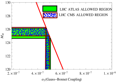
Figure 1: Variation of zeroth mode KK mass of bulk scalar field with respect to Gauss-Bonnet coupling ($\alpha_{5}$ ). The green shaded and the blue dotted region shows the LHC ATLAS and CMS allowed region of recently observed Higgs at 125 GeV respectively. Here we use all the statistical and systematic errors of the corresponding detectors of LHC for the numerical estimations. For numerical estimations throughout the paper we fix the compactification radius $r_{c}\approx 1$ in the Planck unit.

To proceed further we assume that the spontaneous symmetry breaking mechanism is taking place in 5D by which, the bulk scalar, bulk fermions and gauge bosons are getting mass. Such scenarios have been elaborately discussed in various earlier works rizzo ; pomarol ; okada ; cheng ; ssg1 ; ssg2 . This scenario has the advantage of accommodating positive brane tension of the visible brane and thus ensures stability of the proposed model ssg2 ; ssg3 .

The mass generation procedure can be described from action of the scalar $\xi$ and its coupling with a fermion $\eta$ as:

$$\displaystyle S_{\xi}\supset\int d^{5}x\sqrt{-g_{(5)}}\left\{\frac{1}{2}\left[g^{AB}D_{A}{\xi}(x,y)D_{B}{\xi}(x,y)\right.\right.$$

$$\left.\left.\displaystyle-m^{2}_{\xi}{\xi}^{2}(x,y)\right]+\lambda_{\xi}{\xi}^{4}(x,y)+y_{\eta}\xi\eta\bar{\eta}\right\}$$ (5)

where the covariant derivative is defined as:

$$D_{A}\equiv\partial_{A}+ig_{1}^{\prime}T^{b}W^{b}_{A}+ig_{2}^{\prime}YB_{A}$$ (6)

which is the suitable linear combination of W and B vector fields give rise to $W^{+},W^{-},Z$ and photon fields in 5D. Additionally, in Eq (6) $g_{1}^{\prime}$ and $g_{2}^{\prime}$ signifies the unbroken ${\cal SU}(2)$ and ${\cal U}(1)$ gauge couplings while $T^{b}$ and $Y$ are the corresponding generators of the gauge groups associated with the W and B vector boson fields. Here $m^{2}_{\xi}$ signifies the mass parameter of the field $\xi$ before spontaneous symmetry breaking, $\lambda_{\xi}$ be the self-interaction strength of scalar ($\xi$) and $y_{\eta}$ represents the Yukawa coupling. Now after symmetry breaking mechanism by writing, $\xi=v_{1}+\bf H$ and $\eta=\Psi$ the 5D action stated in Eq (Collider constraints on Gauss-Bonnet coupling in warped geometry model) can be recast as:

$$\displaystyle S_{\bf SSB}\supset\int d^{5}x\sqrt{-g_{(5)}}\left\{\frac{1}{2}\left[g^{AB}\partial_{A}{\bf H}(x,y)\partial_{B}{\bf H}(x,y)\right.\right.$$

$$\left.\left.\displaystyle+m^{2}_{h}{\bf H}^{2}(x,y)\right]+m_{f}\Psi\bar{\Psi}+y_{\eta}{\bf H}\Psi\bar{\Psi}+h_{w}{\bf H}W^{+}W^{-}\right\}$$ (7)

Most importantly, in the effective 4D counterpart the photon field has to be massless and also it appears that for such a physical prescription, the 5D mass parameter must be zero. Here $v_{1}$ is the VEV of $\xi$ field. $h_{w}$ which characterizes the coupling strength of the ${\bf H}W^{+}W^{-}$ interaction and the physical mass parameter for the scalar and fermionic degrees of freedom after spontaneous symmetry breaking can be written as:

$$\displaystyle m^{2}_{h}=-\frac{m^{2}_{\xi}}{2\lambda_{\xi}},~{}~{}~{}\displaystyle m_{f}=y_{\eta}v_{1},~{}~{}~{}\displaystyle h_{w}=\frac{1}{2}{g_{1}^{\prime}}^{2}v_{1}.$$ (8)

Further the recent observation of a resonance named Higgs at the LHC ATLAS07 ; CMS03 with mass around 125 GeV will help us to compare the new particle to the zeroth mode of the KK mass spectrum of scalar degrees of freedom (${\bf H}_{0}$) in presence of GB coupling. This zeroth mode scalar mass obtained as Choudhury:2013jhep :

$$\begin{array}[]{llll}\displaystyle m_{s}=M_{H}\approx\left(\frac{1}{2}\sqrt{4+\frac{m_{h}^{2}}{k^{2}_{\alpha}}}-\frac{3}{4}\right)\pi k_{\alpha}e^{-k_{\alpha}r_{c}\pi}.\end{array}$$ (9)

In Fig (1) we have demonstrated the behaviour of zeroth mode Higgs like scalar mass appearing in the 4D effective version of the warped geometry model with respect to the GB coupling by the red curve. We have also shown the present status of our proposed model after applying the Higgs mass constraint $M^{CMS}_{H}=(125.7\pm 0.3)^{+0.3}_{-0.3}$ GeV CMSAp and $M^{ATLAS}_{H}=(125.5\pm 0.2)^{+0.5}_{-0.6}$ GeV ATLASMa obtained from ATLAS & CMS data by green shaded and blue dotted region respectively. This allows to put a stringent bound on the GB coupling within $4.6\times 10^{-7}<\alpha_{5}<5.1\times 10^{-7}$ as shown in a very tiny region in Fig (1). Additionally, this also satisfies the constraint on GB coupling obtained from Eq (4).

Next we apply the constraint on GB coupling from different decay channels of Higgs where interactions between various KK zero modes play a crucial role. The effective field theory provides such interactions below UV cut-off. Most importantly at the tree level the scalar KK zero mode is not coupled to any of the gauge boson. However at loop level such coupling indeed appears signifying some possible non-trivial consequences. Additionally, it appears that the total decay width is dominated by the contribution of two fermion decay mode at the tree level. For computing the higgs decay to two photons and two gluons the contribution of top quark triangle loop diagram as well as decay into two W boson channels are considered. We also assume that the effects from the other fermionic degrees of freedom in the loop level analysis are sufficiently small because the other quarks and leptons being much lighter will contribute much less in the decay width and branching ratio. Here we use a generic ansatz for KK decomposition for the bulk 5D fields as,

$$\begin{array}[]{lllll}\displaystyle{\bf K}_{\beta}(x,y)=\sum^{\infty}_{n=0}{\bf K}^{(n)}_{\beta}(x)~{}\frac{\chi^{(n)}_{{\bf K}_{\beta}}(y)}{\sqrt{r_{c}}}.\end{array}$$ (10)

where $\beta=\ 1(\text{Higgs like scalar}),\ 2(\text{Left handed fermion}),\\ \ 3(\text{Abelian gauge field}),\ 4(\text{Non-abelian gauge field})$.

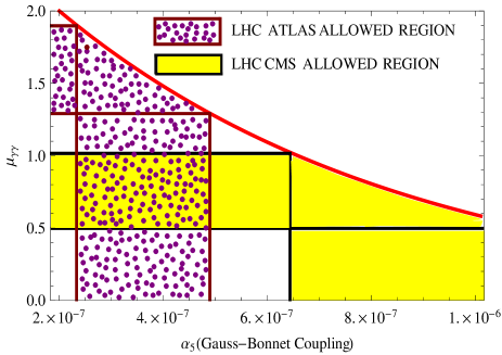
Figure 2: Variation of $\mu_{\gamma\gamma}$ for $H\rightarrow\gamma\gamma$ with respect to Gauss-Bonnet coupling ($\alpha_{5}$) for AdS space ($\Lambda_{5}<0$). The yellow shaded region shows the LHC CMS allowed region. The violet dotted region represents the LHC ATLAS allowed region for our proposed model.

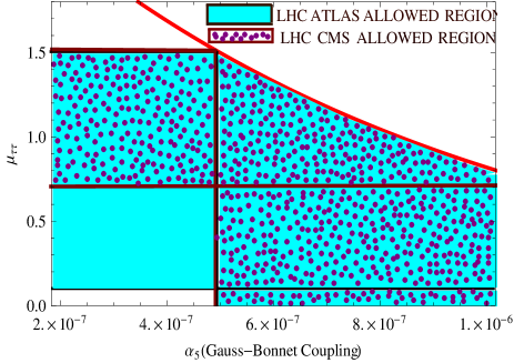
Figure 3: Variation of $\mu_{\gamma\gamma}$ for $H\rightarrow\tau{\bar{\tau}}$ with respect to Gauss-Bonnet coupling ($\alpha_{5}$) for AdS space ($\Lambda_{5}<0$). The aqua shaded region shows the LHC ATLAS allowed region. The violet dotted region represents the LHC CMS allowed region for our proposed model.

In the present context to find the Yukawa interaction between two KK zero mode fermions and one scalar degrees of freedom, the vertex factor of the 4D counterpart of the 5D action after KK decomposition can be obtained from:

$${\cal Q}^{000}:=\int^{+\pi}_{-\pi}dy~{}e^{4A(y)}\chi^{(0)}_{{\bf K}_{1}}(y)\chi^{(0)\star}_{{\bf K}_{2}}(y)\chi^{(0)}_{{\bf K}_{2}}(y).$$ (11)

Similarly the interaction between two KK zero mode fermions and one massless abelian/non-abelian gauge boson can be obtained from

$$\begin{array}[]{lllll}\displaystyle{\cal G}^{000}:=\int^{+\pi}_{-\pi}dy~{}e^{A(y)}\chi^{(0)\star}_{{\bf K}_{2}}(y)\chi^{(0)}_{{\bf K}_{3/4}}(y)\chi^{(0)}_{{\bf K}_{2}}(y).\end{array}$$ (12)

Also the interaction of one KK zeroth mode scalar and two KK zero mode massive non-abelian gauge bosons can be obtained from:

$$\begin{array}[]{lllll}\displaystyle{\cal W}^{000}:=\int^{+\pi}_{-\pi}dy~{}\chi^{(0)}_{{\bf K}_{1}}(y)\chi^{(0)}_{{\bf K}_{4}}(y)\chi^{(0)}_{{\bf K}_{4}}(y)\end{array}$$ (13)

and the interaction strength of a vertex of one photon zero mode with 2 massive weak boson zero modes can be expressed as:

$$\begin{array}[]{lllll}\displaystyle{\cal A}^{000}:=\int^{+\pi}_{-\pi}dy~{}\chi^{(0)}_{{\bf K}_{3}}(y)\chi^{(0)}_{{\bf K}_{4}}(y)\chi^{(0)}_{{\bf K}_{4}}(y).\end{array}$$ (14)

In the interaction integrals for KK zero mode as stated in Eq (11) & Eq (14) we use the following expressions for the KK zero mode wave functions for the different field contents:

$$\chi^{(0)}_{{\bf K}_{\beta}}(y)=\left\{\begin{array}[]{ll}\displaystyle N_{s}&\mbox{ \it for $\beta=1$}\\ \displaystyle N_{f}e^{-\nu A(y)}&~{}\mbox{\it for $\beta=2$}\\ \displaystyle\frac{1}{\sqrt{2\pi}}&~{}\mbox{\it for $\beta=3,4$}.\end{array}\right.$$ (15)

where $N_{f}=\sqrt{\frac{2\left[e^{(1-2\nu)k_{\alpha}r_{c}\pi}-1\right]}{\left(1-2\nu\right)k_{\alpha}r_{c}}}$ and $N_{s}=\sqrt{\frac{k_{\alpha}r_{c}}{1-e^{-2k_{\alpha}r_{c}\pi}}}$. Also we use $\nu=\frac{m_{f}}{k_{\alpha}}$, where $m_{f}$ is defined in Eq (8). Finally the effective 4D coupling for the interactions stated in Eq (11) & Eq (14) can be written as:

$$F_{\cal Q} = y_{\eta}{\cal Q}^{000}=\frac{2N_{f}^{2}N_{s}}{m_{f}r_{c}}\sinh{(m_{f}r_{c}\pi)},$$ (16)

$$F_{\cal G} = \frac{g_{f}{\cal G}^{000}}{\sqrt{r_{c}}}=\frac{g_{f}N_{f}^{2}}{\sqrt{2\pi r_{c}}}\frac{\sinh{(k_{\alpha}-2m_{f})\pi r_{c}}}{(k_{\alpha}-2m_{f})r_{c}},$$ (17)

$$F_{\cal W} = h_{w}{\cal W}^{000}=h_{w}N_{s},$$ (18)

$$F_{\cal A} = \frac{g_{e}}{r_{c}^{\frac{3}{2}}}{\cal A}^{000}=\frac{g_{e}}{\sqrt{2\pi r_{c}^{3}}}$$ (19)

where $y_{\eta}$ is the 5D Yukawa coupling, $g_{f}$ is the gauge coupling which is different for different gauge groups and $g_{e}$ is the 5D gauge coupling of spontaneously broken ${\cal U}(1)$.

So obtaining the couplings of the zeroth mode massive scalar boson with other particles we calculate the decay width and the branching ratio in various channels. We can also obtain the production cross section of this particle, which can be the resonances found at 125 GeV describing the SM Higgs boson. Using these results together we can get the expression for the LHC observable $\mu$ parameter (described in the Appendix) for di-photon and dilepton channels. Hence comparing the derived $\mu$ parameter with the experimental results obtained from the CMS and ATLAS one can get further stringent constraints on GB coupling for suitable choice of other parameters.

The Higgs like scalar candidate in our proposed model couple to the KK zeroth mode of other massive bulk fermions and massive gauge bosons at the tree level. Different SM fermion masses can be obtained from different 5D bulk fermion mass parameter. Using these inputs we can compute the decay width of the dacay channel of the scalar KK zero mode to various fermion KK zero modes using the vertex function explicitly mentioned in Eq. (16). Using Eq (8,16), the decay width to ith fermionic channel can be written as

$$\Gamma({\bf H}_{0}\rightarrow f_{i}\bar{f_{i}})=\frac{N_{c}}{8\pi}F^{2}_{{\cal Q}_{i}}m_{s}\left(1-\frac{4m_{f_{i}}^{2}}{m_{s}^{2}}\right)^{\frac{3}{2}}$$ (20)

where $i=1,2,3,4$ correspond to the tau lepton, bottom, charm and top quark, analogous to SM fermions, respectively and also $m_{f_{i}}$ represent the different fermion masses of the “i”th species. $N_{c}$ is 3 for all quarks and 1 for leptons. Summimg over the all leading contributions total fermionic decay width can be written as:

$$\Gamma_{\text{fer}}\approx\sum^{4}_{i=1}\Gamma({\bf H}_{0}\rightarrow f_{i}\bar{f_{i}})=\frac{N_{c}m_{s}}{8\pi}\sum^{4}_{i=1}F^{2}_{{\cal Q}_{i}}\left(1-\frac{4m_{f_{i}}^{2}}{m_{s}^{2}}\right)^{\frac{3}{2}}.$$ (21)

Another considerable contribution comes from the scalar decay to the zeroth mode massive $W^{+},W^{-}$ bosons. Here the Higgs like scalar mostly decays to one on-shell ($W^{+}$) and another off-shell ($W^{-\ast}$) W bosons. This off shell W further decays to fermion pairs. This is expressed as:

$$\Gamma({\bf H}_{0}\rightarrow W^{+}W^{-\ast})=\frac{m_{s}^{4}}{48m_{W}^{2}}F_{\cal W}^{2}F_{\cal G}^{2}T\left(m_{W}^{2},m_{s}^{2}\right)$$ (22)

where the explicit form of $T(m_{W}^{2},m_{s}^{2})$ is given by:

$$\begin{array}[]{llll}\displaystyle T\left(m_{W}^{2},m_{s}^{2}\right)=\int d(k^{2})\frac{[\lambda^{\frac{3}{2}}(m_{W}^{2},k^{2},m_{s}^{2})+\lambda^{\frac{1}{2}}(m_{W}^{2},k^{2},m_{s}^{2})\frac{12k^{2}m_{W}^{2}}{m_{s}^{4}}]}{(k^{2}-m_{W}^{2})^{2}+{\Gamma}_{W}^{2}m_{W}^{2}}\end{array}$$ (23)

with a new parameter

$$\lambda(m_{W}^{2},k^{2},m_{s}^{2})=\left(1-\frac{m_{W}^{2}}{m_{s}^{2}}-\frac{k^{2}}{m_{s}^{2}}\right)^{2}-\frac{4m_{W}^{2}k^{2}}{m_{s}^{4}}.$$ (24)

Additionally, $m_{W}$ and $\Gamma_{W}$ characterizes the mass and decay width respectively corresponding to the KK zero mode W boson. Consequently the total decay width of this scalar can be written as:

$$\Gamma_{\text{total}}\approx\Gamma({\bf H}_{0}\rightarrow W^{+}W^{-\ast})+\Gamma_{\text{fer}}.$$ (25)

It is important to mention here that in the present context the scalar decay in to two photons loop diagrams of both zeroth mode W boson and top quark will contributing. However the contribution from the W loops are found to be dominant. Taking into account only the dominant contribution from the W in computing the decay width we get:

$$\Gamma({\bf H}_{0}\rightarrow\gamma\gamma)=\frac{m_{s}^{3}}{3456{\pi}^{5}m_{W}^{4}}F^{2}_{\cal A}F^{2}_{\cal W}\left[U\left(\frac{4m_{W}^{2}}{m_{s}^{2}}\right)\right]^{2}$$ (26)

where the functional form of $U(q)$ is given by:

$$U\left(q\right)=\left[2+3q+3q\left(2-q\right)\left\{sin^{-1}\frac{1}{\sqrt{q}}\right\}^{2}\right].$$ (27)

with $q=\frac{4m_{W}^{2}}{m_{s}^{2}}>1$. Further, to calculate the decay width of the zeroth mode scalar to two massless gluons which are zeroth KK modes of the non abelian fields with strong gauge interaction strength, the vertex factor of the two fermion zero mode (mainly top like one) and one gauge boson zero mode is to be taken into account. Consequently the digluon decay width can be computed as:

$$\Gamma({\bf H}_{0}\rightarrow gg)=\frac{m_{f_{4}}^{2}N_{g}}{256\pi^{5}m_{s}}F_{{\cal Q}_{4}}^{2}F^{4}_{{\cal G}_{g}}\left[D\left(\frac{m_{f_{4}}^{2}}{m_{s}^{2}}\right)\right]^{2}$$ (28)

where $N_{g}$ is the colour factor which is 8 for gluon channel. In this context, we define a new function:

$$D\left(z\right)=\left[1+\left(1-4z\right)\left\{sin^{-1}\frac{1}{2\sqrt{z}}\right\}^{2}\right]$$ (29)

with $z=\frac{m_{f_{4}}^{2}}{m_{s}^{2}}>1/4$. In LHC gluon-gluon fusion is the dominant mechanism for the scalar production. Differential production cross section of the scalar considered here in a hadronic collider like LHC is given as hh ,

$$\displaystyle\frac{d\sigma}{dy}(p\bar{p}\rightarrow{\bf H}_{0}+X)=\frac{{\pi}^{2}\Gamma[{\bf H}_{0}\rightarrow\text{gg}]}{8m_{s}^{3}}g_{p}(x_{p},m_{s}^{2})g_{\bar{p}}(x_{\bar{p}},m_{s}^{2})$$ (30)

where we define gluon momentum fraction as:

$$\displaystyle x_{p}=\frac{m_{s}e^{y}}{\sqrt{s}},~{}~{}~{}~{}x_{\bar{p}}=\frac{m_{s}e^{-y}}{\sqrt{s}}.$$ (31)

In Eq (30) $y$ represents the rapidity of the scalar, $g_{p}(x_{p},M_{s}^{2})$ is the gluon distribution function in proton evaluated at the gluon momentum fraction $x_{p}$ and $\sqrt{s}$ signifies the beam energy. Assuming the rapidity to be same for both the scalar and the SM Higgs, the ratio of the production cross section in the $\mu$ parameter can be written only as the ratio of the gluon-gluon decay width of this scalar to the Higgs width in that channel. Substituting all of these inputs in Eq (33) (Please see the appendix), we can write the explicit expression for the LHC observable $\mu$ parameter.

Implication of the recent LHC results in diphoton and dilepton decay channels of the Higgs like scalar in this model are explicitly shown in Fig. (2) and Fig. (3) respectively. The allowed regions which are obtained for the 5D GB coupling ($\alpha_{5}$), in these representative figures are also consistent with the phenomenological bound of $\alpha_{5}$ that we have obtained from the Higgs mass constraints. For the ${\bf H}_{0}\rightarrow\gamma\gamma$ decay channel in ATLAS, a region with $2.3\times 10^{-7}<\alpha_{5}<4.9\times 10^{-7}$ is allowed and this region contains the region that we have already obtained from the Higgs mass constraint. But CMS shows a slightly shifted region of $\alpha_{5}>6.4\times 10^{-7}$ than the allowed one. As CMS and ATLAS results differ a bit in this particular channel, no strict constraint can be found to determine the allowed region. With more data coming in the next run of the LHC we can pinpoint the allowed region for $\alpha_{5}$ in the diphoton channel. For the ${\bf H}_{0}\rightarrow\tau{\bar{\tau}}$ decay channel the experimental upper limits on the observed $\mu$ parameter value both in CMS and ATLAS allows the region with $\alpha_{5}>4.8\times 10^{-7}$. This region contains some part of the region allowed by the diphoton channel data and Higgs mass. But in this channel experimental ranges for the $\mu$ parameter are much broader indicating lesser statistical accuracy. This clearly implies that lower limits on the $\mu$ parameter are unable to constraint the upper bound of $\alpha_{5}$ in ${\bf H}_{0}\rightarrow\tau{\bar{\tau}}$ channel. It is expected that more data will help to give stronger upper bound of $\alpha_{5}$ in this channel. Now combining the constraints from all the three cases,namely, $\mu$ parameter values in the ${\bf H}_{0}\rightarrow\gamma\gamma$ and ${\bf H}_{0}\rightarrow\tau{\bar{\tau}}$ decay channels and mass of the resonance discovered near 125 GeV we can constrain the allowed region of $\alpha_{5}$ within $4.8\times 10^{-7}<\alpha_{5}<5.1\times 10^{-7}$. Additionally, this bound also satisfies the criterion obtained from viscosity-entropy ratio as mentioned in Eq (4).

To summarize, we say that the perturbative higher order gravity correction to Einstein’s gravity can also be examined through collider experimental tests. Using the tools mentioned in this paper one can directly check the validity of a higher order gravity or any modified gravity model and also constrain the couplings associated with such higher order gravity corrections. Thus, in this work, by applying the requirements for the warping solution of the metric, we have explicitly shown that for Gauss-Bonnet (GB) gravity, the associated two-loop coupling is always positive and less than $1/4$. Further, imposing the phenomenological constraint from Higss dilepton and diphoton decay channels and also from possible Higgs mass constraint at 125 GeV we obtain a stringent bound on the GB coupling which satisfies the above criteria as well. This result is consistent with similar bounds obtained from solar system constraint ssg4 . This analysis therefore determines the signature of GB coupling and brings out the phenomenological constraint on the value of this parameter in the context of recent LHC experiment.

Appendix

The $\mu$ parameter is designed for comparison of the number of events obtained from a decaying particle to that of the SM expectation. For more than one decay channels present branching ratio (BR) of a particle, X, to any channel $l_{1}l_{2}$ is defined as:

$$BR(X\rightarrow l_{1}l_{2})=\frac{\Gamma(X\rightarrow l_{1}l_{2})}{\Gamma(X\rightarrow\text{all decay channels})}$$ (32)

where $\Gamma(X\rightarrow l_{1}l_{2})=\text{Decay width of}~{}(X\rightarrow l_{1}l_{2})$. Now total production cross section of a particle multiplied by its branching ratio to a decay channel and the luminosity present in the experiment gives us the number of decay products from the signal. So for the diphoton channel in Higgs search the $\mu$ parameter of the model can be expressed as:

$$\mu=\frac{\Sigma({\bf pp}\rightarrow{\bf H}_{0})}{\Sigma({\bf pp}\rightarrow{\bf H_{SM}})}\times\frac{BR({\bf H}_{0}\rightarrow\gamma\gamma)}{BR(\bf H_{SM}\rightarrow\gamma\gamma)}$$ (33)

for fixed collider luminosity. Here $\Sigma$ represents the production cross section, ${\bf H_{SM}}$ signifies the SM Higgs and ${\bf H}_{0}$ is used for zeroth KK mode Higgs like particle in the warped geometry model proposed in Eq (1). Similar expression appears for the dilepton channel.

References

- (1) H. Davoudiasl, J. L. Hewett and T. G. Rizzo, Phys. Lett. B 473 (2000) 43 [arXiv:hep-ph/9911262]; H. Davoudiasl, J. L. Hewett and T. G. Rizzo, Phys. Rev. D 63 (2001) 075004 [arXiv:hep-ph/0006041].
- (2) A. Pomarol, Phys. Lett. B 486 (2000) 153 [arXiv:hep-ph/9911294].
- (3) S. Chang, J. Hisano, H. Nakano, N. Okada and M. Yamaguchi, Phys. Rev. D 62 (2000) 084025 [arXiv:hep-ph/9912498].
- (4) S. J. Huber and Q. Shafi, Phys. Rev. D 63 (2001) 045010.
- (5) P. Dey, B. Mukhopadhyaya and S. SenGupta, Phys. Rev. D 81 (2010) 036011 [arXiv:0911.3761 [hep-ph]].
- (6) A. Das, R. S. Hundi and S. SenGupta, Phys. Rev. D 83 (2011) 116003 [arXiv:1105.1064 [hep-ph]].
- (7) S. Choudhury and S. SenGupta, JHEP 02 (2013) 136, [arXiv:1301.0918 [hep-th]].
- (8) L. Randall and R. Sundrum, Phys. Rev. Lett. 83 (1999) 3370, [arXiv:hep-ph/9905221].
- (9) L. Randall and R. Sundrum, Phys. Rev. Lett. 83 (1999) 4690, [arXiv:hep-th/9906064].
- (10) U. Maitra, B. Mukhopadhyaya and S. SenGupta, arXiv:1307.3018 [hep-ph].
- (11) J. E. Kim, B. Kyae and H. M. Lee, Phys. Rev. D 62 (2000) 045013 [arXiv:hep-ph/9912344].
- (12) J. E. Kim, B. Kyae and H. M. Lee, Nucl. Phys. B 582 (2000) 296 [arXiv:hep-th/0004005].
- (13) S. Choudhury and S. SenGupta, arXiv:1306.0492 [hep-th].
- (14) M. Brigante, H. Liu, R. C. Myers, S. Shenker and S. Yaida, Phys. Rev. D 77 (2008) 126006, [arXiv:0712.0805 [hep-th]].
- (15) G. Policastro, D T. Son and A. O. Starinets, Phys. Rev. Lett. 87 (2001) 081601, [arXiv:hep-th/0104066].
- (16) A. Buchel and J. T. Liu, Phys. Rev. Lett. 93 (2004) 090602, [arXiv:hep-th/0311175].
- (17) P. Kovtun, D. T. Son and A. O. Starinets, Phys. Rev. Lett. 94 (2005) 111601, [arXiv:hep-th/0405231].
- (18) Combined measurements of the mass and signal strength of the Higgs-like boson with the ATLAS detector using up to 25 fb−1 of proton-proton collision data [ATLAS Collaboration], ATLAS-CONF-2013-014.
- (19) Combination of standard model Higgs boson searches and measurements of the properties of the new boson with a mass near 125 GeV [CMS Collaboration], CMS-PAS-HIG-13-005.
- (20) S. Das, D. Maity and S. Sengupta, JHEP 05 (2008) 042 [arXiv:0711.1744 [hep-th]].
- (21) ATLAS Collaboration Phys. Lett. B 716 (2012) 1, [arXiv:1207.7214 [hep-ex]].
- (22) CMS Collaboration JHEP 06 (2013) 081, [arXiv:1303.4571 [hep-ex]].
- (23) J. F. Gunion, H. E. Haber, G. L. Kane and S. Dawson, “The Higgs Hunter’s Guide,” Front. Phys. 80, 1 (2000).
- (24) S. Chakraborty and S. Sengupta, arXiv:1208.1433 [gr-qc].