The Mid-Infrared Extinction Law in the Large Magellanic Cloud
DRAFT:   

Abstract

Based on the photometric data from the Spitzer/SAGE survey and with red giants as the extinction tracers, the mid-infrared (MIR) extinction laws in the Large Magellanic Cloud (LMC) are derived for the first time in the form of $A_{\lambda}/A_{{\rm K_{S}}}$, the extinction in the four IRAC bands (i.e., [3.6], [4.5], [5.8] and [8.0]$\,{\rm\mu m}$) relative to the 2MASS ${\rm K_{S}}$ band at 2.16$\,{\rm\mu m}$. We obtain the near-infrared (NIR) extinction coefficient to be $E({\rm J}-{\rm H})/E({\rm H}-{\rm K_{S}})\approx 1.29\pm 0.04$ and $E({\rm J}-{\rm K_{S}})/E({\rm H}-{\rm K_{S}})\approx 1.94\pm 0.04$. The wavelength dependence of the MIR extinction $A_{\lambda}/A_{\rm K_{S}}$ in the LMC varies from one sightline to another. The overall mean MIR extinction is $A_{[3.6]}/A_{\rm K_{S}}\approx 0.72\pm 0.03$, $A_{[4.5]}/A_{\rm K_{S}}\approx 0.94\pm 0.03$, $A_{[5.8]}/A_{\rm K_{S}}\approx 0.58\pm 0.04$, and $A_{[8.0]}/A_{\rm K_{S}}\approx 0.62\pm 0.05$. Except for the extinction in the IRAC [4.5] band which may be contaminated by the 4.6$\,{\rm\mu m}$ CO gas absorption of red giants (which are used to trace the LMC extinction), the extinction in the other three IRAC bands show a flat curve, close to the Milky Way $R_{V}=5.5$ model extinction curve (where $R_{V}$ is the optical total-to-selective extinction ratio). The possible systematic bias caused by the correlated uncertainties of ${\rm K_{S}}-\lambda$ and ${\rm J}-{\rm K_{S}}$ is explored in terms of Monte-Carlo simulations. It is found that this could lead to an overestimation of $A_{\lambda}/A_{\rm K_{S}}$ in the MIR.

1 Introduction

The Large Magellanic Cloud (LMC) is a low-metalicity irregular dwarf galaxy and a satellite of the Milky Way (MW). Since the metallicity of the LMC (which is only $\,{\sim}$1/4 of that of the MW; Russell & Dopita 1992) is similar to that of galaxies at red shifts $z\sim 1$ (Dobashi et al., 2008), it offers opportunities to study the dust properties in distant low-metallicity extragalactic environments by studying the extinction properties of the LMC.

The wavelength dependence of interstellar extinction – “interstellar extinction law (or curve)” – is one of the primary sources of information about the interstellar grain population (Draine, 2003). In the MW, the interstellar extinction laws in the ultraviolet (UV) and visual wavelength ranges vary from sightline to sightline, and can be characterized by the optical total-to-selective extinction ratio ${R_{V}}\equiv{A_{V}}/{E({\rm B-V})}$ (Cardelli et al., 1989), where ${E({\rm B-V})}={A_{B}}-{A_{V}}$ is the interstellar reddening, ${A_{V}}$ is the extinction at the visual ($V$; $\lambda_{V}\approx 5500\,{\rm\AA}$) band, and ${A_{B}}$ is the extinction at the blue ($B$; $\lambda_{B}\approx 4400\,{\rm\AA}$) band. The regional variations of the UV/visual extinction curves (i.e., the variations of the ${R_{V}}$ values) reflect the variations in dust size: larger ${R_{V}}$ values indicate the predominance of larger grains (Draine, 2003). However, the infrared (IR) interstellar extinction laws of the MW, which also vary from one sightline to another, cannot be simply represented by the single ${R_{V}}$ parameter. Many recent studies show that there does not exist a “universal” near-infrared (NIR) extinction law for the MW (Fitzpatrick & Massa, 2009; Gao et al., 2009). Moreover, the observationally-determined mid-infrared (MIR) extinction law shows a flat curve while classical dust models for the diffuse interstellar medium (ISM) predict a much steeper curve, with a pronounced minimum at $\,{\sim}$7$\,{\rm\mu m}$ (Draine, 1989).

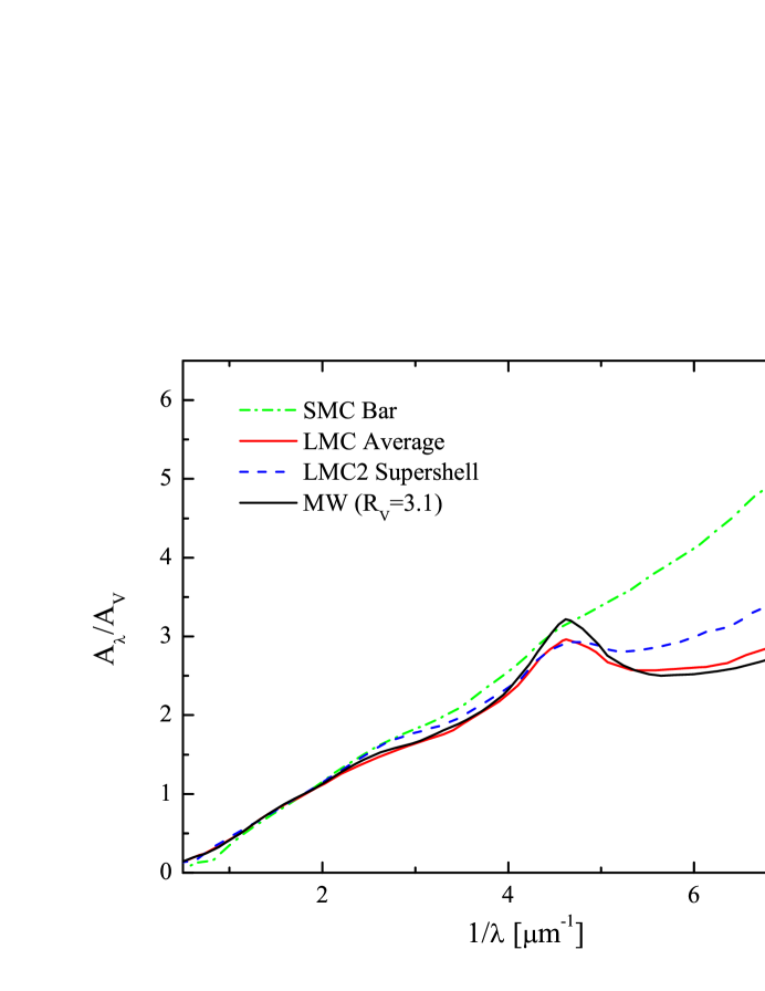
Figure 1: Comparison of the MW (black solid), LMC (red solid), and SMC (green dot-dashed) extinction curves. Also shown is the LMC2 supershell extinction curve (blue dashed). The MW extinction curve is calculated from the CCM parameterization with ${R_{V}}=3.1$. The LMC and SMC extinction curves are taken from Gordon et al. (2003).

Due to its low metallicity, the dust quantity (relative to H) in the LMC is expected to be lower than that of the MW because there is less raw material (i.e., heavy elements) available for making the dust. The (relative) lack of the dust-making raw material could prevent the dust in the LMC from growing and hence the dust in the LMC may be smaller than the MW dust. Furthermore, the star-formation activity in the LMC could destroy the dust. Therefore, one would naturally expect the dust size distribution and extinction curve in the LMC to differ from that of the MW. As illustrated in Figure 1, the Galactic interstellar extinction curve rises from the NIR to the near-UV with a broad absorption bump at about $\lambda^{-1}\approx 4.6\mu{\rm m}^{-1}$ ($\lambda\approx 2175\,{\rm\AA})$, and continues rising steeply into the far-UV (Draine, 2003). In the Small Magellanic Cloud (SMC), the extinction curves of most sightlines display a nearly linear steep rise with $\lambda^{-1}$ and lack the 2175$\,{\rm\AA}$ hump (Lequeux et al., 1982; Prevot et al., 1984). The LMC extinction curve is intermediate between that of the MW and that of the SMC: compared to the Galactic extinction curve, the LMC extinction curve is characterized by a weaker 2175$\,{\rm\AA}$ hump and a stronger far-UV rise (Nandy et al., 1981; Koornneef & Code, 1981; Gordon et al., 2003). Strong regional variations in extinction properties have also been found in the LMC (Clayton & Martin, 1985; Fitzpatrick, 1985, 1986; Gordon & Clayton, 1998; Misselt et al., 1999; Gordon et al., 2003): the sightlines toward the stars inside or near the supergiant shell, LMC 2, which lies on the southeast side of the 30 Doradus star-forming region, have a very weak 2175$\,{\rm\AA}$ hump (Misselt et al., 1999), while the extinction curves for the sightlines toward the stars which are $>$ 500 pc away from the 30 Doradus region are closer to the Galactic extinction curve. Gordon et al. (2003) estimated ${R_{V}}\approx 2.76$ for the LMC 2 supershell and ${R_{V}}\approx 3.41$ for the LMC as a whole. The sightlines outside 30 Doradus have ${R_{V}}\approx 3.2$ (Fitzpatrick, 1986; Gordon & Clayton, 1998; Misselt et al., 1999). Koornneef (1982) had already noticed that the average value of ${R_{V}}$ in the LMC (${R_{V}}\approx 3.01$) is close (within 10%) to that of the MW (${R_{V}}\approx 3.1)$. We note that the CCM parameterization controlled by the single ${R_{V}}$-parameter is not valid for the LMC extinction curve (Gordon et al., 2003), i.e., even the LMC and the MW are close in ${R_{V}}$, their extinction curves differ appreciably.

Koornneef (1982) derived the NIR extinction law of the LMC based on the NIR photometry at the ${\rm J}$, ${\rm H}$, and ${\rm K}$ bands of early type supergiants. He obtained $E(\rm V-{\rm J})/E(\rm B-\rm V)\approx 2.26\pm 0.23$, $E(\rm V-{\rm H})/E(\rm B-\rm V)\approx 2.58\pm 0.27$, and $E(\rm V-{\rm K})/E(\rm B-\rm V)\approx 2.91\pm 0.31$, and argued that the NIR extinction law of the LMC is very similar to that of the MW. Their results correspond to $E({\rm J}-{\rm H})/E({\rm H}-{\rm K_{S}})\approx 1.06$ when converted to the 2MASS photmetric system (Imara & Blitz, 2007). Because of this, the Galactic NIR extinction law is sometimes adopted for the LMC (e.g., Cioni et al. 2000; Imara & Blitz 2007). Using the near-infrared color-excess (NICE) method (Lada et al., 1994), Imara & Blitz (2007) calculated the NIR extinction coefficients of the LMC to be ${A_{V}}/E({\rm H}-{\rm K_{S}})\approx 20.83\pm 0.52$ and ${A_{V}}/E({\rm J}-{\rm H})\approx 17.30\pm 0.46$, corresponding to $E({\rm J}-{\rm H})/E({\rm H}-{\rm K_{S}})\approx 1.20\pm 0.04$, which is roughly consistent with that of Koornneef (1982). We note that although the LMC NIR extinction law is commonly assumed to be universal, Gordon et al. (2003) showed that it also differs between the LMC 2 supershell and the LMC average (see their Table 4).

So far, little efforts have been put into the MIR extinction properties of the LMC due to the paucity of MIR data. Nevertheless, the MIR extinction is not negligible: the LMC optical extinction ${A_{V}}\lesssim 5.0\,{\rm mag}$ (Imara & Blitz, 2007; Dobashi et al., 2008) would imply an appreciable amount of MIR extinction $A_{[3.6]}\lesssim 0.35\,{\rm mag}$ if we take the Galactic ratio of $A_{[3.6]}/{A_{V}}\sim 0.07$ (Gao et al., 2009). With the advent of sensitive IR space facilities (e.g., ISO and Spitzer), the LMC has been mapped in the MIR wavelength bands with high accuracy and this makes the exploration of the LMC MIR extinction possible. In this work, based on the Spitzer/SAGE database, we probe the MIR extinction of the LMC and its regional variations. In §2 we briefly describe the SAGE data used in this work. §3 presents the method adopted to derive the extinction, including the Galactic foreground extinction correction, the LMC sightline selection, and the selection of extinction tracers. §4 reports the derived extinction law and the mean extinction of the LMC. Finally, we summarize our results in §5.

2 Data

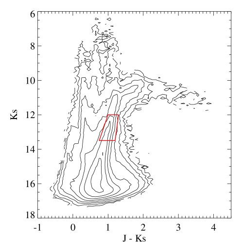
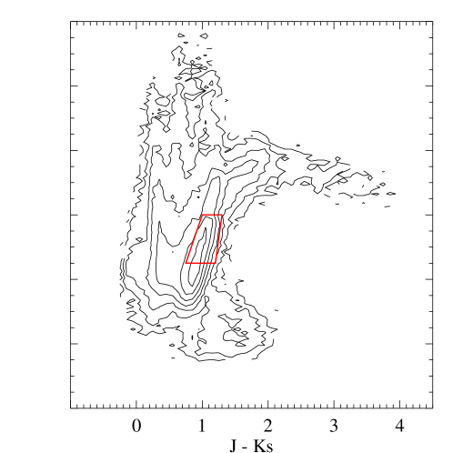
Figure 2: The color-magnitude diagram (CMD) of the LMC. Left panel shows all the sources in the catalog of SAGELMCcatalogIRAC, while the right panel only shows the sources with S/N $\gtrsim$ 5 at all three 2MASS bands and four IRAC bands. The red trapezium shows the region of RGBs, which are candidates for extinction tracers.

The data used in this work were obtained through the Spitzer/SAGE Legacy Program, entitled “Spitzer Survey of the Large Magellanic Cloud: Surveying the Agents of a Galaxy’s Evolution” (Meixner et al., 2006). The SAGE legacy program mapped the LMC at two different epochs (epochs 1 and 2) separated by three months, using the IRAC ([3.6], [4.5], [5.8], and [8.0]$\mu{\rm m}$) and MIPS ([24], [70], and [160]$\mu{\rm m}$) instruments on board the Spitzer Space Telescope. The SAGE Points Source Catalog, named SAGELMCcatalogIRAC, released in September 2009, combined both epochs’ data bandmerged with 2MASS and 6X2MASS all-sky data (Cutri et al., 2003; Cutri & 2MASS Team, 2004). The SAGELMCcatalogIRAC catalog is the SAGE catalog with the highest quality, providing $\,{\sim}$6.4 million point sources at four IRAC bands and three 2MASS or 6X2MASS bands. Faint limits are 18.1, 17.5, 15.3, and 14.2$\,{\rm mag}$ for IRAC [3.6], [4.5], [5.8], and [8.0]$\,{\rm\mu m}$, respectively. The SAGE data also provide the catalogs, such as SAGELMCcatalogMIPS24, SAGELMCcatalogMIPS70 and SAGELMCcatalogMIPS160, which include the sources observed by Spitzer/MIPS at [24], [70], and [160]$\mu{\rm m}$ bands. However, only IRAC data are used in this work for probing the LMC MIR extinction. We only select the sources with a signal-to-noise ratio of S/N $\gtrsim$ 5 at all three 2MASS bands and four IRAC bands (see §3.4 for details on sample selection). Table 1 shows the mean photometric errors for each band in the SAGELMCcatalogIRAC with ${\rm S/N}\gtrsim 5$. Because of the high sensitivity of Spitzer/IRAC, there are $\approx 293935$ sources in SAGELMCcatalogIRAC with S/N $\gtrsim$ 5 at all seven bands (see Figure 2). Additionally, Meixner et al. (2006) estimated that the Galactic foreground stars and background galaxies contribute roughly 18% and 12% of the SAGE catalog sources.

3 Methods and Tracers

3.1 Foreground Extinction

Toward the LMC, many studies have showed that the mean foreground Galactic reddening is $E(\rm B-\rm V)\sim 0.06\,{\rm mag}$ (Bessell et al., 1991; Oestreicher et al., 1995; Staveley-Smith et al., 2003; Imara & Blitz, 2007). Dobashi et al. (2008) estimated the average Galactic extinction across the LMC at the visual band to be ${A_{V}}\sim 0.2\,{\rm mag}$, implying $E(\rm B-\rm V)\sim 0.06\,{\rm mag}$ with the Galactic average value of ${R_{V}}=3.1$.

We correct for the foreground extinction at each 2MASS band, taking the foreground visual extinction to be ${A_{V}}=0.2\,{\rm mag}$ (Dobashi et al., 2008) for all the LMC sources. To see how much the extinction will change using different foreground extinction, we re-calculated the extinction toward CO-186 (30 Doradus). We take the wavelength-dependence of the foreground extinction to be that of the ${R_{V}}=3.1$ Galactic average extinction law (Rieke & Lebofsky, 1985), i.e., $A_{{\rm J}}/{A_{V}}\approx 0.282$, $A_{{\rm H}}/{A_{V}}\approx 0.175$, and $A_{{\rm K_{S}}}/{A_{V}}\approx 0.112$. The mean foreground extinction at each 2MASS band are thus $A_{{\rm J}}\approx 0.056$, $A_{{\rm H}}\approx 0.035$, and $A_{{\rm K_{S}}}\approx 0.022\,{\rm mag}$. The mean foreground extinction derived from the extinction map of Schlegel et al. (1998) are $A_{{\rm J}}\approx 0.055$, $A_{{\rm H}}\approx 0.035$, and $A_{{\rm K_{S}}}\approx 0.021\,{\rm mag}$ (Imara & Blitz, 2007). For the four IRAC bands, the foreground extinction is also corrected by applying the Galactic MIR extinction of $A_{[3.6]}/A_{{\rm K_{S}}}\approx 0.63$, $A_{[4.5]}/A_{{\rm K_{S}}}\approx 0.57$, $A_{[5.8]}/A_{{\rm K_{S}}}\approx 0.49$, and $A_{[8.0]}/A_{{\rm K_{S}}}\approx 0.55$, which were obtained for 131 Spitzer/GLIPMSE fields along the Galactic plane within $|l|<65^{\rm o}$ with red giants and red clump giants (RCGs) as tracers (Gao et al., 2009). Therefore, the mean foreground extinction at the four IRAC bands are $A_{[3.6]}\approx 0.014$, $A_{[4.5]}\approx 0.013$, $A_{[5.8]}\approx 0.011$, and $A_{[8.0]}\approx 0.012$$\,{\rm mag}$, respectively.

3.2 Selection of Regions

As mentioned in §1 the LMC UV/visual extinction exhibits substantial regional variation, particularly among sightlines toward stars in and outside the 30 Doradus region. Little is known about the MIR extinction of the LMC and its variation toward different sightlines, until the Spitzer/SAGE database offers us the unique opportunity. As the MIR extinction is generally small, to probe the MIR extinction efficiently we favor the LMC regions with large ${A_{V}}$ (after all, only these highly obscured regions need to be corrected for IR extinction).

Previous studies have estimated that the mean LMC reddening varies from $E(\rm B-\rm V)\approx 0.10\,{\rm mag}$ to $E(\rm B-\rm V)\approx 0.16\,{\rm mag}$ (see Table 2 in Imara & Blitz 2007). Imara & Blitz (2007) constructed the visual extinction (${A_{V}}$) map and found the mean value of ${A_{V}}$ is $\,{\sim}$0.38$\,{\rm mag}$. Zaritsky et al. (2004) constructed extinction maps for two stellar populations in the central 64 $\rm deg^{2}$ area of the LMC, and derived the average extinction of ${A_{V}}\approx 0.43\,{\rm mag}$ and ${A_{V}}\approx 0.55\,{\rm mag}$ for the cold and hot populations, respectively. Dobashi et al. (2008) developed a new method by using the color of the X percentile reddest stars and derived a new ${A_{V}}$ map of the LMC, which is similar to the integrated intensity of the CO emission as observed by the NANTEN telescope (Fukui et al., 2008).

All these extinction maps showed that the maximum ${A_{V}}$ of the LMC is close to $\,{\sim}$5$\,{\rm mag}$. Since $A_{{\rm K_{S}}}/{A_{V}}\sim 0.1$ (the extinction at the ${\rm K_{S}}$ band relative to ${A_{V}}$), for ${A_{V}}=1\,{\rm mag}$ $A_{{\rm K_{S}}}$ is only $\,{\sim}$0.1$\,{\rm mag}$. The mean measurement uncertainty of the 2MASS survey is $\sim$0.109 mag for the ${\rm K_{S}}$ magnitude (SNR = 1). Therefore, it is necessary to only consider the regions with ${A_{V}}\gtrsim 1\,{\rm mag}$. In addition, the LMC areas containing special structures (such as bar or molecular ridge) and some special interstellar environments also need to be considered in order to probe the variation of MIR extinction among different interstellar environments.

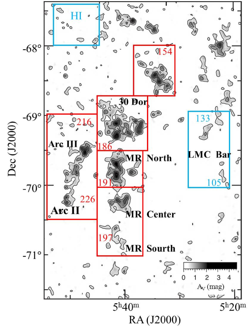
Figure 3: The seven LMC regions selected for studying the LMC MIR extinction. The red boxes show the five regions selected to probe the MIR extinction of the LMC. The two blue boxes show the regions in the LMC bar and in the HI area, where ${A_{V}}$ is smaller than 1$\,{\rm mag}$. The extinction map is taken from Dobashi et al. (2008) (see their Figure 6).

Sakon et al. (2006) investigated the mid- to far-IR emission of the LMC based on the COBE/DIRBE and IRAS Sky Survey Atlas data. In their Figure 12, they illustrated the local structures in the molecular ridge (MR) and the CO arc in the LMC. These structures are associated with the CO molecular clouds, as well as the highly obscured regions in the extinction map derived by Dobashi et al. (2008). Combining Dobashi et al. (2008)’s extinction map and Sakon et al. (2006)’s Figure 12 with the NANTEN ¹²CO map (Fukui et al., 2008), we select five regions with large ${A_{V}}$ in the LMC molecular clouds and MR and arc structures (see the red boxes in Figure 3; in the following we will call these five regions “the first five regions”). Although the average ${A_{V}}$ is smaller than 1$\,{\rm mag}$ or even much smaller, the regions in the LMC bar and HI area (marked as blue boxes in Figure 3) are also considered for comparison. All these seven regions are listed in Table 2 labeled with the structure name and the molecular cloud number.

3.3 Color-Excess Method

The determination of dust extinction is most commonly made by comparing the flux densities of obscured and unobscured pair stars of the same spectral type (Li & Mann, 2012). In this work we adopt the “color-excess” method to obtain the extinction. The “color-excess” method is widely applied to photometric data and can probe deeper than the spectrum-pair method. For doing this, a group of sources which have essentially the same intrinsic color indices (or with very small scattering in the color indices) are chosen. This method calculates the ratio of the two color excesses which can be expressed as following

$$k_{x}\equiv\frac{E(\lambda_{r}-\lambda_{x})}{E(\lambda_{c}-\lambda_{r})}=\frac{(\lambda_{r}-\lambda_{x})_{\rm observed}-(\lambda_{r}-\lambda_{x})_{\rm intrinsic}}{(\lambda_{c}-\lambda_{r})_{\rm observed}-(\lambda_{c}-\lambda_{r})_{\rm intrinsic}}=\frac{A_{r}-A_{x}}{A_{c}-A_{r}}$$ (1)

where $\lambda_{x}$ is the magnitude in the interested band $x$; $\lambda_{r}$ is the magnitude in the reference band $r$ (taken to be the ${\rm K_{S}}$ band in this work); $\lambda_{c}$ is magnitude in the comparison band $c$ (taken to be the J band in this work). Therefore, the extinction ratio of the $\lambda$ band to the ${\rm K_{S}}$ reference band is

$$A_{\lambda}/A_{\rm Ks}=1+k_{\lambda}\left(1-A_{\rm J}/A_{\rm Ks}\right)~{}~{},$$ (2)

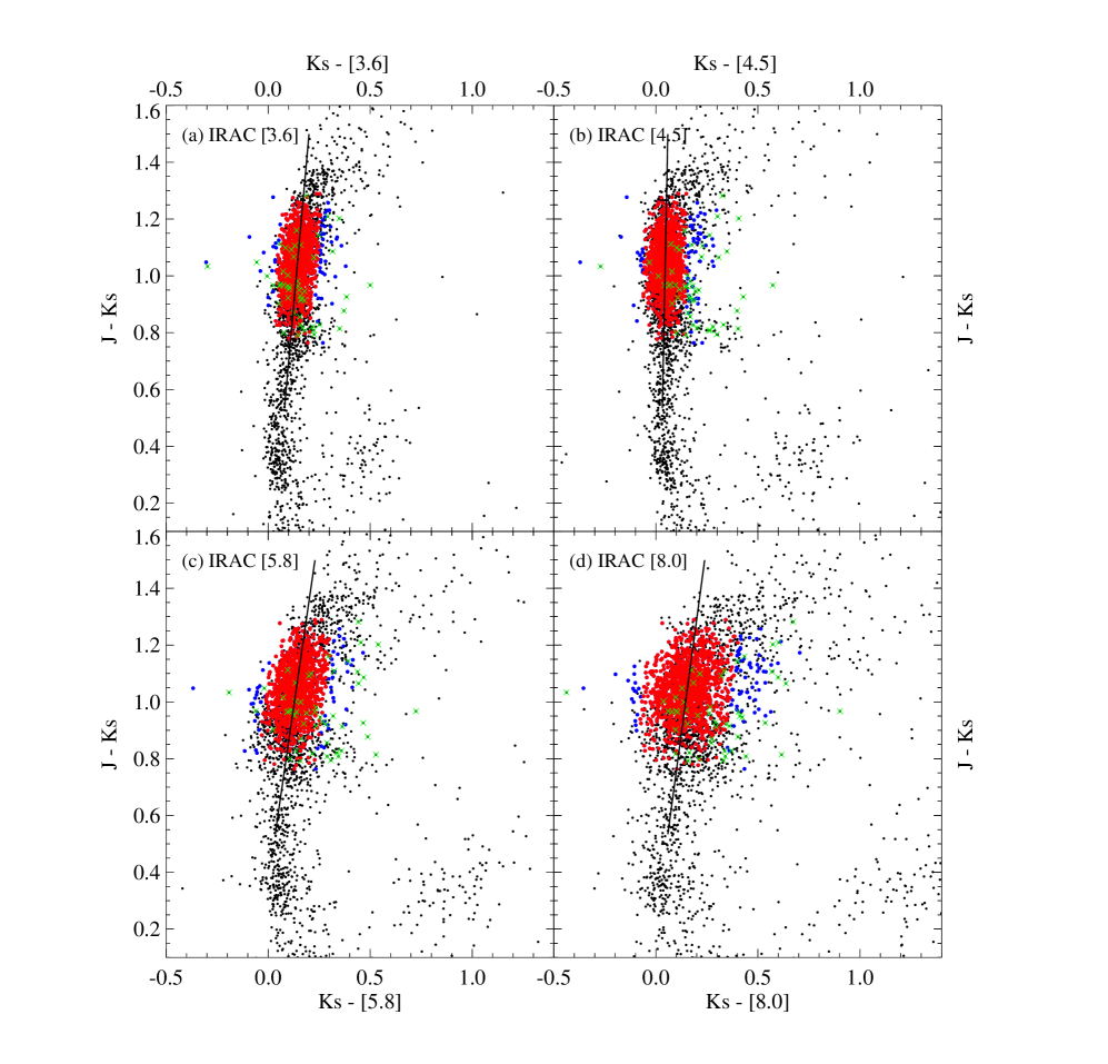
Figure 4: Sample of fitting for the 30 Doradus region (CO-186). The slopes of the black lines are $1/k_{\lambda}$ (see eq. 2 for $k_{\lambda}$, which can be used to derive $A_{\lambda}/A_{\rm Ks}$). Red and blue dots show all RGB sources selected in the 30 Doradus region (CO-186) using the method described in §3.4, while green crosses show the sources in the Region E with $[3.6]-[4.5]>0$ or $[5.8]-[8.0]>0.5$. Only red dots are the RGB sources used in the final fitting after applying the $3\sigma$ principle. Black dots show all the sources with S/N $\gtrsim$ 5 in all seven (2MASS and IRAC) bands in this region.

where $k_{\lambda}$ is used to derive $A_{\lambda}/A_{\rm Ks}$ from $A_{\rm J}/A_{\rm K_{S}}$ and can be obtained by fitting the observed color indices $({\rm K_{S}}-\lambda)_{\rm obs}$ and $(\rm J-{\rm K_{S}})_{\rm obs}$ with a linear line (Jiang et al., 2003, 2006; Gao et al., 2009). The slope of the fitted linear line is $k_{\lambda}$. This is a statistical method as it makes use of a large number of sources and reduces the risk of depending on any individual objects with large uncertainties in the determination of their intrinsic color indices. In Figure 4, we show the samples of fitting for the 30 Doradus region (CO-186).

From eq. 1 and eq. 2, it is seen that the determination of $A_{\lambda}/A_{\rm K_{S}}$ (i.e., the ratio of the $\lambda$-band extinction to the extinction of the reference band ${\rm K_{S}}$) requires the knowledge of $A_{\rm J}/A_{{\rm K_{S}}}$. Gordon et al. (2003) obtained $A_{\rm J}/A_{\rm K_{S}}\approx 2.96$ for the LMC 2 supershell near 30 Doradus. We adopt $A_{\rm J}/A_{\rm K_{S}}=2.96$ since the regions selected for this study are near 30 Doradus (CO-186) (see Figure 3). For the sake of comparison, we also take the Galatcic value of $A_{\rm J}/A_{\rm K_{S}}=2.52$ (Rieke & Lebofsky, 1985) which is often adopted to study the LMC extinction (Cioni et al., 2000; Imara & Blitz, 2007).

3.4 Tracers

In our previous work of probing the variation of the MIR extinction law in the Galactic plane (Gao et al., 2009), red giant branch stars (RGBs) were used as the tracer to study the extinction law at the four IRAC bands. In the IR, red giants are appropriate tracers of interstellar extinction for the following reasons: (i) they have a narrow range of effective temperatures so that the scatter of their intrinsic color indices is small; (ii) they are bright in the IR ($M_{{\rm K_{S}}}\approx-5.0\,{\rm mag}$) and remain visible even suffering large extinction and/or observed from a great distance, even in the LMC.

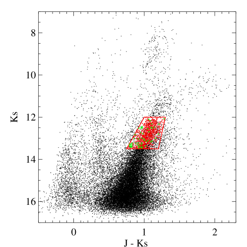
Figure 5: The NIR CMD of the 30 Doradus (CO-186) region. The selected RGB samples are denoted by red dots within the red trapezoid. Left panel shows all the sources with S/N $\gtrsim$ 1 at all three 2MASS bands in the 30 Doradus (CO-186) region from the Spitzer/SAGE IRAC catalog, while the right panel only shows the sources with S/N $\gtrsim$ 5 at all seven bands (three 2MASS bands and four IRAC bands) in the same region. Green crosses show the sources with $[3.6]-[4.5]>0.0$ or $[3.6]-[8.0]>0.5$ in the selected region.

In the LMC, RGB stars are one of the most prominent and well populated features in the color-magnitude diagram (CMD) of stellar populations with ages larger than $\,{\sim}$1.5–2.0 Gyr (Salaris & Girardi, 2005). Nikolaev & Weinberg (2000) performed a morphological analysis on the 2MASS CMD of the LMC and distinguished different populations of stars in the LMC. The populations were identified based on isochrone fitting and matching the theoretical CMD colors of known populations to the observed CMD source density (see Figure 3 and Tables 2, 3 of Nikolaev & Weinberg 2000). Imara & Blitz (2007) selected the sources in Regions E, F, G, H, J, L, and part of Region D of Nikolaev & Weinberg (2000) to derive the extinction map of the LMC. They eliminated Regions A, B, C, and I, which contain much foreground contamination. Although it is free of foreground contamination, Region K is also eliminated because it consists of dusty AGB stars whose large ${\rm J}-{\rm K}$ colors are due to circumstellar dust. However, the sources considered by Imara & Blitz (2007) contain too many different stellar populations. We note that Region E of Nikolaev & Weinberg (2000), located within $12<{\rm K_{S}}<13.5$ and $0.9\lesssim\rm J-Ks\lesssim 1.2$, covers the upper RGB and includes the tip of the RGB. Therefore, we choose a slightly expanded version of Region E to select the RGB stars: the selected region is constrained to $12\leq{\rm K_{S}}\leq 13.5$ and $0.75\leq\rm{\rm J}-{\rm K_{S}}\leq 1.3$ (see Figures 2,5).

However, it should be noted that evolved red giants may have circumstellar dust shells which would cause circumstellar extinction and produce IR emission, hence affecting our understanding of their intrinsic color indices. Additionally, the selected region (Region E) may contain other populations which will affect the extinction determination. For the MW, astronomers commonly use $[3.6]-[4.5]$ $<$ 0.6 and $[5.8]-[8.0]$ $<$ 0.2 as the criteria to exclude the sources with IR excess such as pre-main-sequence stars and asymptotic giant branch (AGB) stars (Flaherty et al., 2007; Gao et al., 2009). For the LMC, Meixner et al. (2006) presented initial results on the epoch 1 data of the Spitzer/SAGE program for a region near N79 and N83, which is near the southwest end of the LMC bar. They adopt a simplified point-source classification to identify three candidate groups – stars without dust, dusty evolved stars, and young stellar objects (YSOs) on the MIR color-color diagrams. In their Figure 11 and Figure 12, Meixner et al. (2006) showed the stars without dust are almost constrained to $[3.6]-[4.5]<0.0$, $[5.8]-[8.0]<0.5$. Therefore, we will also use $[3.6]-[4.5]<0.0$ and $[5.8]-[8.0]<0.5$ in order to reduce the contamination caused by YSOs and AGBs.

In Figures 4 and 5, green crosses show the sources with $[3.6]-[4.5]>0.0$ or $[5.8]-[8.0]>0.5$ in the selected Region E. Figure 5 shows the NIR CMD of the 30 Doradus (CO-186) region, which is one of the selected parts in the LMC. The selected RGB sources are denoted by red dots within the red trapezoid. Left panel shows all the sources with S/N $\gtrsim$ 1 at all three 2MASS bands in the 30 Doradus (CO-186) region from the Spitzer/SAGE IRAC catalog, while the right panel only shows the sources with S/N $\gtrsim$ 5 at all seven bands (i.e., three 2MASS bands and four IRAC bands) in the same region.

The red clump giants (RCGs) are also often used as tracers to probe the IR extinction in the MW. However, RCGs in the LMC are often too faint to be observed (at least in large number). The tip-RGBs in the LMC have ${\rm K_{S}}\approx 12\,{\rm mag}$ (Sakai et al., 2000; Nikolaev & Weinberg, 2000; Salaris & Girardi, 2005; Mucciarelli et al., 2006) and RGBs are within $12<{\rm K_{S}}<16\,{\rm mag}$, while RCG stars have ${\rm K_{S}}\approx 17\,{\rm mag}$ (Alves et al., 2002; Mucciarelli et al., 2006). Therefore, in this work only RGBs are considered as tracers to probe the MIR extinction of the LMC.

4 Results and Discussion

4.1 The NIR Extinction Law

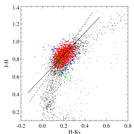
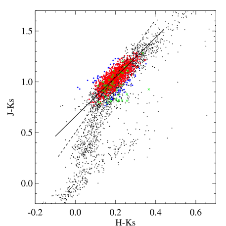
Figure 6: The NIR color-color diagram of the 30 Doradus (CO-186) region. The symbols are the same as those in Figure 4. For this region, the NIR color ratios are $E({\rm J}-{\rm H})/E({\rm H}-{\rm K_{S}})\approx 1.29\pm 0.04$ and $E({\rm J}-{\rm K_{S}})/E({\rm H}-{\rm K_{S}})\approx 1.94\pm 0.04$, which are shown as black solid lines. In the MW, these values are $E({\rm J}-{\rm H})/E({\rm H}-{\rm K_{S}})\approx 1.73$ and $E({\rm J}-{\rm K_{S}})/E({\rm H}-{\rm K_{S}})\approx 2.78$ (Indebetouw et al., 2005), which are shown as black dashed lines.

Imara & Blitz (2007) derived the NIR extinction coefficient of the LMC using the NICE method (Lada et al., 1994) and the NICER (NICE revised) method (Lombardi & Alves, 2001). The NICER technique relies on the mean color of the control group being characteristic of the intrinsic color of the field stars (Imara & Blitz, 2007). They took the mean color of the control group as the intrinsic color of their interested fields, i.e., $({\rm H}-{\rm K})_{\rm intrin}\equiv 0.16\pm 0.09\,{\rm mag}$. However, their control groups include the sources in Regions E, F, G, H, J, L, and part of D of Nikolaev & Weinberg (2000), so that the dispersion around the mean control color was larger than that of RGB stars. Based on the selected RGB stars, we fit the NIR color-color diagrams of ${\rm J}-{\rm H}$ versus ${\rm H}-{\rm K_{S}}$ and ${\rm J}-{\rm K_{S}}$ versus ${\rm H}-{\rm K_{S}}$ with the IDL robust linear fit procedure. Our results show that the average NIR extinction coefficient for the first five LMC regions listed in Table 2 is consistent with previous studies, i.e., $E({\rm J}-{\rm H})/E({\rm H}-{\rm K_{S}})\approx 1.29\pm 0.04$ and $E({\rm J}-{\rm K_{S}})/E({\rm H}-{\rm K_{S}})\approx 1.94\pm 0.04$ (see Table 3). In Figure 6, we show the NIR color-color diagrams and the fits for the 30 Doradus region (CO-186). Green crosses show the sources with $[3.6]-[4.5]>0.0$ or $[3.6]-[8.0]>0.5$ in the selected Region E of 30 Doradus. It efficiently reduces the contamination of YSOs and AGBs, and prevents from distorting the fit by excluding these sources.

As far as individual parts of the LMC are concerned, the NIR extinction coefficients vary among different regions of the LMC. However, the variation is relatively small among the first five regions listed in Table 2 which have molecular clouds and for which ${A_{V}}$ is large. For comparison, Table 3 also shows the NIR extinction coefficients for the LMC bar and HI region. Because of their small amounts of extinction, we believe that the results (for the LMC bar and HI region) are less certain (compared to those for the first five regions listed in Table 2) and the IR extinction cannot be detected efficiently.

4.2 The MIR Extinction Law

In Table 3, the color ratios of $E({\rm K_{S}}-\lambda)/E({\rm J}-{\rm K_{S}})$ are shown for the four IRAC bands. Based on these color ratios and taking $A_{{\rm J}}/A_{{\rm K_{S}}}=2.96$ (Gordon et al., 2003), we calculate the relative extinction $A_{\lambda}/A_{{\rm K_{S}}}$. In Table 4 we show the extinction at each IRAC band (relative to that of the ${\rm K_{S}}$ band) for the selected regions of the LMC. We note that only the first five regions listed in Table 1 are considered in obtaining the average MIR extinction of the LMC (although the MIR extinction toward the LMC bar and HI region are also derived and tabulated in Table 4).

As a whole, with RGBs as the extinction tracers, the mean MIR extinction ratios of the LMC are $A_{[3.6]}/A_{\rm K_{S}}\approx 0.72\pm 0.03$, $A_{[4.5]}/A_{\rm K_{S}}\approx 0.94\pm 0.03$, $A_{[5.8]}/A_{\rm K_{S}}\approx 0.58\pm 0.04$, and $A_{[8.0]}/A_{\rm K_{S}}\approx 0.62\pm 0.05$. In Figure 7, we show the MIR extinction of the LMC together with the MW model extinction curves of ${R_{V}}=3.1$ and ${R_{V}}=5.5$ (Weingartner & Draine, 2001). The red filled squares show the average MIR extinction of the LMC at the four IRAC bands, while the red error bars show the maximum and minimum extinction of the five selected fields, demonstrating the regional variation of MIR extinction in the LMC. If the extinction at [4.5]$\,{\rm\mu m}$ is excluded (see §4.3), the extinction at [3.6], [5.8] and [8.0]$\,{\rm\mu m}$ of the LMC consists a flat curve, close to that of the MW model extinction curve of ${R_{V}}=5.5$, lacking the deep minimum around 7$\,{\rm\mu m}$ predicted from the ${R_{V}}=3.1$ model. The extinction at [4.5]$\,{\rm\mu m}$ is well above the ${R_{V}}=5.5$ model extinction curve and also well exceeds the extinction at the other three IRAC bands. As far as individual sightlines are concerned, the wavelength dependence of the LMC MIR extinction $A_{\lambda}/A_{{\rm K_{S}}}$ also varies from one sightline to another (see Table 3 and 4).

In the literature the NIR extinction law of the MW has often been used to represent that of the LMC (Cioni et al., 2000; Imara & Blitz, 2007). For comparison, we have also calculated the MIR extinction of the LMC taking the Galactic value of $A_{\rm J}/A_{\rm K_{S}}=2.52$ (Rieke & Lebofsky, 1985). The results are also tabulated in Table 4: the extinction is larger than that derived with the LMC2 supershell value of $A_{\rm J}/A_{\rm K_{S}}=2.96$ (Gordon et al., 2003) by $\,{\sim}$8%, 2%, 17%, and 15% at [3.6], [4.5], [5.8], and [8.0], respectively.

4.3 The Extinction at [4.5]$\,{\rm\mu m}$

As clearly seen in Figure 7 and Table 4, the mean extinction of the 4.5$\,{\rm\mu m}$ IRAC band $A_{[4.5]}/A_{{\rm K_{S}}}\approx 0.94\pm 0.03$ is not only much higher than that of the other three IRAC bands, but also much larger than that of the Galactic plane average of $A_{[4.5]}/A_{{\rm K_{S}}}\approx 0.63\pm 0.01$ derived from the RGBs tracers (Gao et al., 2009).

In Galactic and extragalactic dense clouds various ice features have been observed, including the 3.1$\,{\rm\mu m}$ feature due to the O–H stretching mode of H₂O ice as well as a number of weaker features at 4.27$\,{\rm\mu m}$ due to the C–O stretching mode of CO₂ ice, at 4.67$\,{\rm\mu m}$ due to the C–O stretching mode of CO ice, and at 6.02$\,{\rm\mu m}$ due to the H–O–H bending mode of H₂O ice. In this work, the selected sightlines are mostly located in molecular clouds, therefore, it is not unreasonable, at a first glance, to attribute the [4.5] excess extinction to $\rm CO_{2}$ and CO ices in the LMC dense clouds. Observational, experimental and theoretical studies have shown that CO and CO₂ ices could efficiently form both in quiescent clouds and in active star-forming regions (e.g., see Nummelin et al. 2001; Ruffle & Herbst 2001; Mennella et al. 2004; Whittet et al. 2007; Oba et al. 2010; Noble et al. 2011; Ioppolo et al. 2011; Garrod & Pauly 2011). Whittet et al. (2007) found a threshold of ${A_{V}}$ $\approx$ 4.3$\pm$1.0, 6.7$\pm$1.6$\,{\rm mag}$ respectively for the detection of CO₂ and CO ices in the Taurus dark cloud complex; for H₂O ice, the detection threshold is ${A_{V}}$ $\approx$ 3.2$\pm$0.1$\,{\rm mag}$ (Whittet et al., 2001b). With ${A_{V}}<5\,{\rm mag}$ for the selected LMC regions, it is unlikely for these regions to have CO₂/H₂O or CO/H₂O much higher than that of the MW.

To examine whether the ice (particularly CO₂ and, to a less degree, CO) absorption bands could account for the [4.5] excess extinction, we approximate the 3.05, 4.27, 4.67 and 6.02$\,{\rm\mu m}$ bands respectively from H₂O, CO₂, CO, and H₂O ices as four Drude profiles. The extinction due to these four ice bands is

$$A_{\lambda}({\rm ice})=1.086\,N_{\rm H_{2}O}\sum\limits_{j=1}^{4}\frac{A_{j}\times\left[{\rm X}_{j}/{\rm H_{2}O}\right]\times E_{j}\times 2\gamma_{j}/\pi}{\left(\lambda-\lambda_{j}^{2}/\lambda\right)^{2}+\gamma_{j}^{2}}$$ (3)

where $\lambda_{j}$, $\gamma_{j}$, $A_{j}$ are the peak wavelength, FWHM, and strength of the $j$-th ice absorption band, respectively (see Table 5); $N_{\rm H_{2}O}$ is the H₂O ice column density; ${\rm X}_{j}/{\rm H_{2}O}$ is the abundance of the ice species ${\rm X}_{j}$ relative to H₂O ice in typical dense clouds; $E_{j}$ is the “enhancement” factor for species ${\rm X}_{j}$ (i.e., ${\rm X}_{j}/{\rm H_{2}O}$ is increased by a factor of $E_{j}$ in order for the ice absorption bands to account for the [4.5] excess extinction). Finally, we add $A_{\lambda}({\rm ice})$ to $\left(A_{\lambda}/A_{{\rm K_{S}}}\right)_{\rm WD}$, the WD01 extinction curve (with ${R_{V}}=3.1$ or 5.5) (Weingartner & Draine, 2001) and then convolve with the Spitzer/IRAC filter response functions.

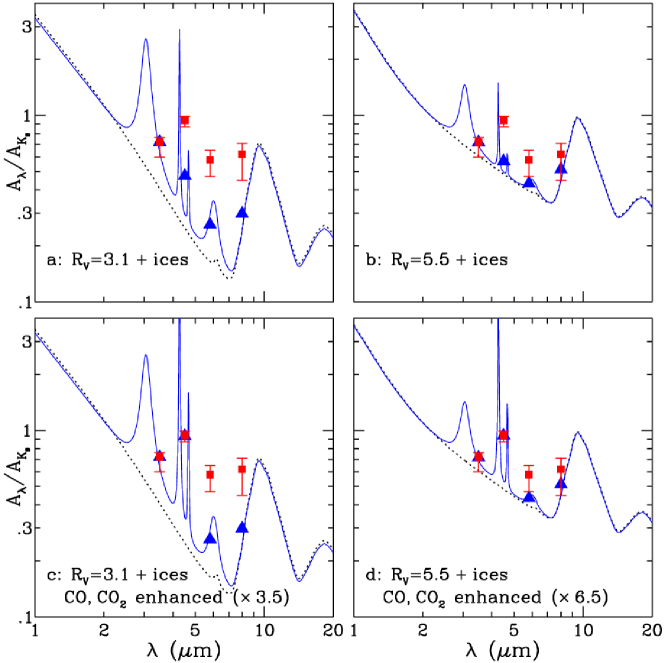
Figure 8: Comparison of the LMC mean MIR extinction at the four IRAC bands (red filled squares) with the ${R_{V}}=3.1$ and ${R_{V}}=5.5$ models (black dotted lines) combined with the 3.05 and 6.02$\,{\rm\mu m}$ absorption bands of H₂O ice, the 4.27$\,{\rm\mu m}$ band of CO₂ ice, and the 4.67$\,{\rm\mu m}$ band of CO ice (blue solid lines). Blue filled triangles are the ${R_{V}}=3.1$ or ${R_{V}}=5.5$ model curve plus the ice absorption bands convolved with the Spitzer/IRAC filter functions. Upper panels (a, b): the abundances of CO and CO₂ ices are taken to be that of typical dense clouds (i.e., ${\rm CO/H_{2}O=0.25}$, ${\rm CO_{2}/H_{2}O=0.21}$). Bottom panels (c, d): the abundances of CO and CO₂ ices are enhanced relative to their typical values in dense clouds.

The H₂O ice abundance (i.e., $N_{\rm H_{2}O}$) is constrained not to exceed the IRAC [3.6] extinction. With ${\rm CO/H_{2}O\approx 0.25}$ and ${\rm CO_{2}/H_{2}O\approx 0.21}$, typical for quiescent dense clouds (Whittet, 2003; Gibb et al., 2004; Boogert et al., 2011), CO and CO₂ are not capable of accounting for the [4.5] excess extinction. If we are forced to attribute the [4.5] excess extinction to CO and CO₂, we will have too much H₂O ice and the resulting extinction at [3.6] would be too high. If we fix the H₂O ice abundance at what is required by the [3.6] extinction, in order for CO and CO₂ to explain the [4.5] excess extinction, we have to enhance their abundances (relative to their typical abundances in dense clouds) by a factor of $E_{\rm CO}=E_{\rm CO_{2}}\approx 3.5$ for ${R_{V}}=3.1$ and $E_{\rm CO}=E_{\rm CO_{2}}\approx 6.5$ for ${R_{V}}=5.5$ (see Figure 8).

We note that although the extinction at [3.6] and [4.5] is well fitted by the ${R_{V}}=3.1$ model combined with ices, it could not account for the flat extinction at [5.8] and [8.0]. In contrast, the ${R_{V}}=5.5$ model together with ices could closely explain the MIR extinction at all four IRAC bands provided that the abundances of CO and CO₂ ices are increased by a factor of $\,{\sim}$6.5 from their typical abundances in dense clouds. However, the required CO and CO₂ abundances are unrealistically too high: ${\rm CO/H_{2}O\approx 1.7}$ and ${\rm CO_{2}/H_{2}O\approx 1.4}$ for ${R_{V}}=5.5$.

The origin of the [4.5] excess extinction remains unclear. Some red giants have circumstellar envelopes rich in CO gas which absorbs at 4.6$\,{\rm\mu m}$ (Bernat, 1981). With red giants as a tracer of the mid-IR extinction, the 4.6$\,{\rm\mu m}$ absorption feature of their CO gas would result in an overestimation of the IRAC [4.5] extinction. It is worth exploring whether the CO gas absorption of red giants could account for the [4.5] excess extinction.

4.4 Systematic Bias

As discussed in §3.3, in deriving the IR extinction law, the ${\rm K_{S}}-\lambda$ vs. ${\rm J}-{\rm K_{S}}$ color-color diagram is fitted to obtain the slope $k_{\lambda}$ (see eq.1 and eq.2). Since ${\rm K_{S}}-\lambda$ and ${\rm J}-{\rm K_{S}}$ both employ the ${\rm K_{S}}$ band photometry and therefore may have correlated uncertainties, there could be systematic bias in determining $k_{\lambda}$ and $A_{\lambda}/A_{\rm J}$.

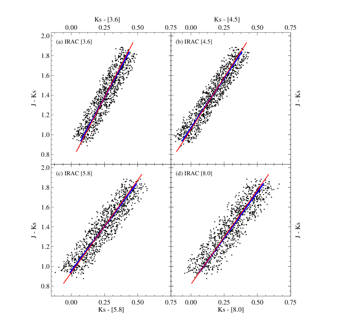
Figure 9: A sample of Monte-Carlo simulation with $N=1000$, ${R_{V}}=3.1$, $\left(A^{\rm mc}_{{\rm J}}\right)_{\rm max}=1.5\,{\rm mag}$, and the mean photometric uncertainties for the sources with ${\rm S/N}>5$ in all three 2MASS bands and four IRAC bands. The thick blue lines show the simulated colors of the obscured sources (but no errors are added to these sources). The black dots show the colors of the simulated, obscured, error-added sources. The red lines fit the ${\rm J}-{\rm K_{S}}$ vs. ${\rm K_{S}}-\lambda$ color-color diagram for the simulated, obscured, error-added sources.

To evaluate the possible systematic bias, we perform simple Monte-Carlo simulations. Using CMD 2.5 (Bressan et al., 2012), we generate stellar isochrones and take a stellar atmosphere model of $T_{\rm eff}=4,004{\rm K}$, $Z=0.019$, ${\rm log\,g}\,=\,1.28$ for the simulated stars. The stellar absolute magnitudes are approximatly $-4.068$, $-4.850$, $-5.006$, $-5.079$, $-4.941$, $-4.997$, and $-5.068\,{\rm mag}$ in ${\rm J}$, ${\rm H}$, ${\rm K_{S}}$, [3.6], [4.5], [5.8], and [8.0] bands, respectively. We then apply a random amount of extinction to obscure a large number of stars. The stars are taken to be identical and have the same absolute magnitudes. Let $A^{\rm mc}_{\lambda}$ be the amount of extinction to which the stars are subject. We take the stars to be obscured by $A^{\rm mc}_{\lambda}$, with $A^{\rm mc}_{\lambda}$ being a random number between 0 and $\left(A^{\rm mc}_{\lambda}\right)_{\rm max}$. We take the ${\rm J}$ band as the basis wavelength and assume the extinction at other wavelengths to follow either the MW ${R_{V}}=3.1$ model curve or the MW ${R_{V}}=5.5$ model curve of Weingartner & Draine (2001). The thick blue lines in Figure 9 shows the simulated color indices for a large number of stars ($N=1,000$) in the ${\rm J}-{\rm K_{S}}$ vs. ${\rm K_{S}}-\lambda$ color-color diagram. The stars are obscured by the ${R_{V}}=3.1$-type extinction with $\left(A^{\rm mc}_{\rm J}\right)_{\rm max}=1.5\,{\rm mag}$.

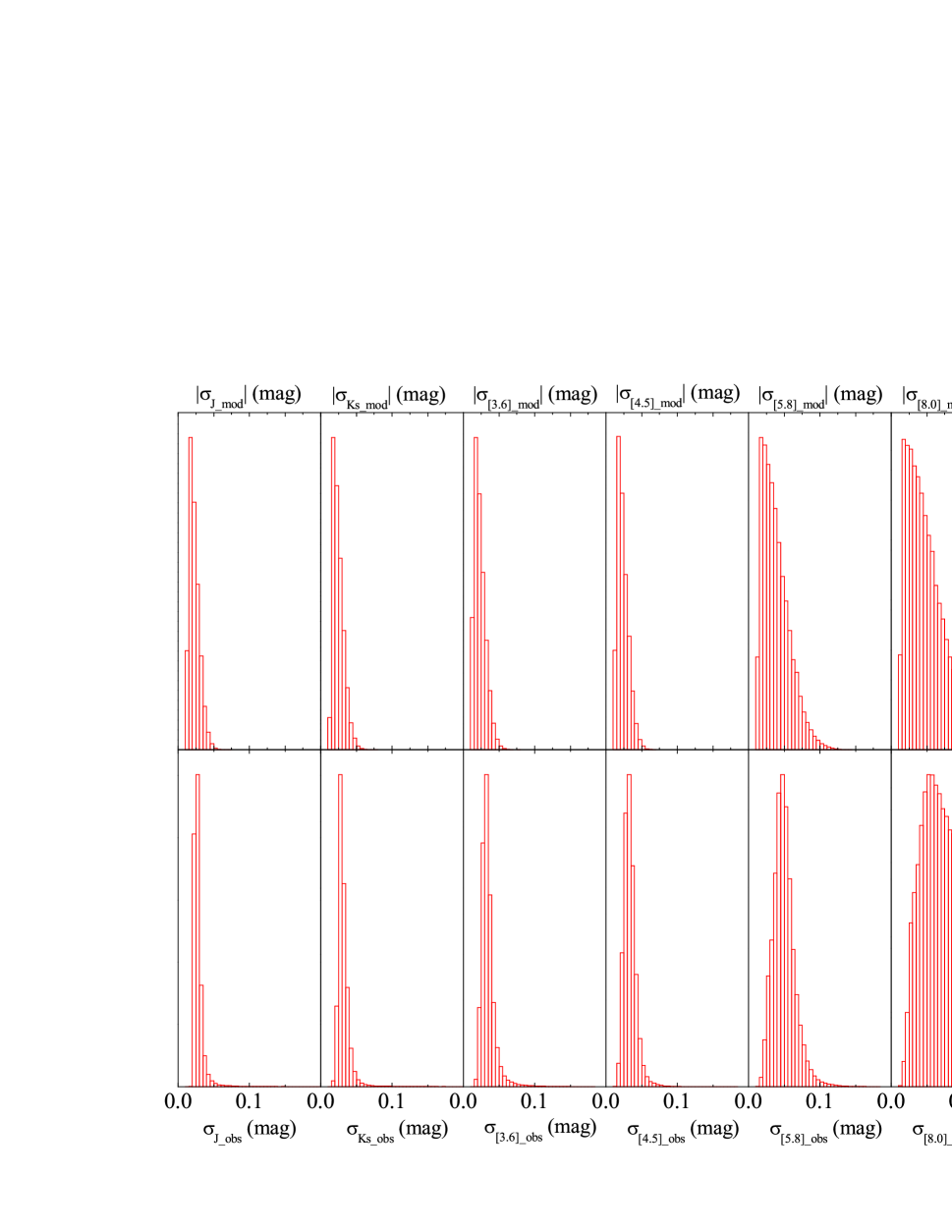
Figure 10: Comparison of the simulation errors (upper panel) with the photometric uncertainties for the sources with ${\rm S/N}>5$ at all three 2MASS bands and four IRAC bands (lower panel; see Table 1).

We then add errors to the obscured stellar magnitudes based on the uncertainties of the SAGELMCcatalogIRAC (see Table 1). The errors are simulated to follow a Poisson distribution, with their mean values being the mean photometric uncertainties of the sources with ${\rm S/N}>5$ in all seven bands in SAGELMCcatalogIRAC (see Figure 10 for a comparison of the simulated errors with the mean photometric uncertainties). In Figure 9, the simulated, error-added sources are shown as black dots in the ${\rm J}-{\rm K_{S}}$ vs. ${\rm K_{S}}-\lambda$ color-color diagram. The slope for the resulting ${\rm J}-{\rm K_{S}}$ vs. ${\rm K_{S}}-\lambda$ diagram (black dots) is fitted (see the red lines in Figure 9). Figure 9 shows that the extinction laws derived from the obscured, error-added sources are different from the original ones adopted to obscure the stars: the derived slopes of $k_{\lambda}$, i.e. $E({\rm K_{S}}-\lambda)/E({\rm J}-{\rm K_{S}})$, are all smaller than the simulated ones, and therefore the derived $A_{\lambda}/A_{\rm Ks}$ ratios are overestimated.

We have examined the effects of (i) the level of obscuration $\left(A^{\rm mc}_{\rm J}\right)_{\rm max}$, (ii) the number of stars $N$, (iii) the amount of error, and (iv) the extinction-type which is employed to obscure the stars. As shown in Table 6, the level of obscuration $\left(A^{\rm mc}_{\rm J}\right)_{\rm max}$ dominates the systematic bias which decreases with the increasing of $\left(A^{\rm mc}_{\rm J}\right)_{\rm max}$. For $\left(A^{\rm mc}_{\rm J}\right)_{\rm max}\gtrsim 5\,{\rm mag}$ the systematic bias becomes negligible.

Gordon et al. (2003) derived $A_{\rm J}/{A_{V}}\approx 0.299$ for the lines of sight toward the LMC2 supershell near 30 Doradus. With ${A_{V}}\lesssim 5\,{\rm mag}$, we obtain $A_{\rm J}\lesssim 1.5\,{\rm mag}$. Therefore, the MIR $A_{\lambda}/A_{\rm Ks}$ ratios may have been overestimated and the color ratios $E({\rm K_{S}}-\lambda)/E({\rm J}-{\rm K_{S}})$ may have been underestimated. With $N=1,000$, $\left(A^{\rm mc}_{\rm J}\right)_{\rm max}=1.5\,{\rm mag}$, and a ${R_{V}}=3.1$-type extinction (see the fifth row in Table 6), we perform a Monte-Carlo simulation to assess the possible systematic bias caused by the correlated uncertainties of ${\rm K_{S}}-\lambda$ and ${\rm J}-{\rm K_{S}}$. We find that the extinction ratios $A_{\lambda}/A_{\rm J}$ derived in §4.2 could be overestimated by $\,{\sim}$6%, 10%, 16% and 9% at [3.6], [4.5], [5.8] and [8.0], respectively. The corrected extinction $A_{\lambda}/A_{\rm Ks}$ will be $A_{[3.6]}/A_{\rm K_{S}}\approx 0.68\pm 0.03$, $A_{[4.5]}/A_{\rm K_{S}}\approx 0.84\pm 0.03$, $A_{[5.8]}/A_{\rm K_{S}}\approx 0.49\pm 0.04$, and $A_{[8.0]}/A_{\rm K_{S}}\approx 0.57\pm 0.05$.

5 Conclusions

The Spitzer/SAGE IRAC catalog provides us a unique opportunity to study the MIR extinction of the LMC. We select five fields with large optical extinction (${A_{V}}>1\,{\rm mag}$) to explore the MIR extinction of the sightlines toward these regions. Taking $A_{\rm J}/A_{\rm K_{S}}=2.96$ (Gordon et al., 2003) and using RGB stars as tracers, we find that:

1. The NIR color-color diagrams are fitted to derive the NIR extinction coefficients: $E({\rm J}-{\rm H})/E({\rm H}-{\rm K_{S}})\approx 1.29\pm 0.04$ and $E({\rm J}-{\rm K_{S}})/E({\rm H}-{\rm K_{S}})\approx 1.94\pm 0.04$, which are consistent with earlier studies (Koornneef, 1982; Imara & Blitz, 2007). The corresponding color ratios for the MW are $E({\rm J}-{\rm H})/E({\rm H}-{\rm K_{S}})\approx 1.73$ and $E({\rm J}-{\rm K_{S}})/E({\rm H}-{\rm K_{S}})\approx 2.78$ (Indebetouw et al., 2005).

2. At the four IRAC bands, the derived mean MIR extinction of the LMC are $A_{[3.6]}/A_{\rm K_{S}}\approx 0.72\pm 0.03$, $A_{[4.5]}/A_{\rm K_{S}}\approx 0.94\pm 0.03$, $A_{[5.8]}/A_{\rm K_{S}}\approx 0.58\pm 0.04$, and $A_{[8.0]}/A_{\rm K_{S}}\approx 0.62\pm 0.05$. The corresponding extinction ratios for the MW are $A_{[3.6]}/A_{\rm K_{S}}\approx 0.63\pm 0.01$, $A_{[4.5]}/A_{\rm K_{S}}\approx 0.57\pm 0.03$, $A_{[5.8]}/A_{\rm K_{S}}\approx 0.49\pm 0.03$, and $A_{[8.0]}/A_{\rm K_{S}}\approx 0.55\pm 0.03$ (Gao et al., 2009).

3. The LMC extinction at [3.6], [5.8] and [8.0]$\,{\rm\mu m}$ is consistent with a flat curve, close to that of the MW model extinction curve predicted by the interstellar grain model of ${R_{V}}=5.5$. Similar to that of the MW, the LMC MIR extinction law exhibits appreciable regional variations.

4. The extinction at [4.5] is much higher than that of the other three IRAC bands. It cannot be explained in terms of the 4.27$\,{\rm\mu m}$ absorption band of $\rm CO_{2}$ ice and the 4.67$\,{\rm\mu m}$ absorption band of CO ice. It may be caused by the 4.6$\,{\rm\mu m}$ absorption feature of CO gas in the circumstellar envelopes of red giants which are used to trace the IR extinction.

5. The derived MIR extinction $A_{\lambda}/A_{\rm J}$ may be overestimated because of the correlated uncertainties of ${\rm K_{S}}-\lambda$ and ${\rm J}-{\rm K_{S}}$ which could affect the determination of $k_{\lambda}$, the slope of the ${\rm K_{S}}-\lambda$ vs. ${\rm J}-{\rm K_{S}}$ color-color diagram. With this systematic bias taken into account, the derived extinction ratios $A_{\lambda}/A_{\rm J}$ could be overestimated by $\,{\sim}$6%, 10%, 16% and 9% at [3.6], [4.5], [5.8] and [8.0], respectively.

Table 1: The mean photometric uncertainties in SAGELMCcatalogIRAC

$\lambda$	${\rm J}$	${\rm H}$	${\rm K_{S}}$	[3.6]	[4.5]	[5.8]	[8.0]
$\langle\sigma\rangle$ ($\,{\rm mag}$)	0.0280	0.0296	0.0316	0.0343	0.0330	0.0492	0.0658

Table 2: The LMC sightlines explored in this work

No.	Field Name	$\rm RA_{min}$	$\rm RA_{max}$	$\rm DEC_{min}$	$\rm DEC_{max}$	Note
		(deg)	(deg)	(deg)	(deg)
1	CO-154	82.5	84.0	-68.7	-68.0	CO Cloud 154
2	30 Doradus	83.5	86.0	-69.5	-68.7	Star-Forming Region, CO Cloud 186
3	MR North	84.0	86.0	-70.0	-69.5	Molecular Ridge North, CO Cloud 191
4	MR South	84.0	86.0	-71.0	-70.0	MR Center and South, CO Cloud 197
5	Arcs	86.0	88.0	-70.5	-69.0	Arc II and Arc III, CO Cloud 216, 226
6	LMC Bar	80.0	82.0	-70.0	-69.0	CO Cloud 133, 105
7	HI Region	86.0	88.0	-68.5	-67.5	HI Region

Table 3: The IR extinction coefficients of the LMC

Field	$\frac{E({\rm J}-{\rm H})}{E({\rm H}-{\rm K_{S}})}$	$\frac{E({\rm J}-{\rm K_{S}})}{E({\rm H}-{\rm K_{S}})}$	$\frac{E({\rm K_{S}}-[3.6])}{E({\rm J}-{\rm K_{S}})}$	$\frac{E({\rm K_{S}}-[4.5])}{E({\rm J}-{\rm K_{S}})}$	$\frac{E({\rm K_{S}}-[5.8])}{E({\rm J}-{\rm K_{S}})}$	$\frac{E({\rm K_{S}}-[8.0])}{E({\rm J}-{\rm K_{S}})}$
CO-154	1.310$\pm$0.053	1.936$\pm$0.049	0.145$\pm$0.018	0.031$\pm$0.020	0.211$\pm$0.025	0.204$\pm$0.036
30 Doradus	1.286$\pm$0.039	1.944$\pm$0.037	0.124$\pm$0.013	0.028$\pm$0.014	0.202$\pm$0.019	0.187$\pm$0.029
MC North	1.271$\pm$0.046	1.934$\pm$0.042	0.206$\pm$0.016	0.068$\pm$0.012	0.269$\pm$0.024	0.280$\pm$0.035
MC South	1.279$\pm$0.026	1.932$\pm$0.025	0.120$\pm$0.009	0.006$\pm$0.009	0.180$\pm$0.012	0.150$\pm$0.018
Arcs	1.310$\pm$0.030	1.957$\pm$0.029	0.124$\pm$0.010	0.013$\pm$0.010	0.196$\pm$0.013	0.146$\pm$0.018
Average	1.291$\pm$0.039	1.941$\pm$0.036	0.144$\pm$0.013	0.029$\pm$0.013	0.212$\pm$0.019	0.193$\pm$0.027
HI region	1.138$\pm$0.050	1.706$\pm$0.047	0.054$\pm$0.018	-0.078$\pm$0.019	0.087$\pm$0.026	0.075$\pm$0.033
LMC bar	1.185$\pm$0.019	1.782$\pm$0.018	0.125$\pm$0.007	-0.025$\pm$0.007	0.192$\pm$0.010	0.166$\pm$0.013

Table 4: The MIR extinction law of the LMC

Field	$A_{[3.6]}/A_{\rm K_{S}}$	$A_{[4.5]}/A_{\rm K_{S}}$	$A_{[5.8]}/A_{\rm K_{S}}$	$A_{[8.0]}/A_{\rm K_{S}}$
CO-154	0.72$\pm$0.04	0.94$\pm$0.04	0.59$\pm$0.05	0.60$\pm$0.07
30 Doradus	0.76$\pm$0.03	0.95$\pm$0.04	0.60$\pm$0.04	0.63$\pm$0.06
MC North	0.60$\pm$0.03	0.87$\pm$0.02	0.47$\pm$0.04	0.45$\pm$0.07
MC South	0.76$\pm$0.02	0.99$\pm$0.02	0.65$\pm$0.02	0.71$\pm$0.04
Arcs	0.76$\pm$0.02	0.97$\pm$0.02	0.62$\pm$0.03	0.71$\pm$0.04
Average	0.72$\pm$0.03	0.94$\pm$0.03	0.58$\pm$0.04	0.62$\pm$0.05
Average	0.68$\pm$0.02	0.84$\pm$0.02	0.49$\pm$0.03	0.57$\pm$0.04
Average	0.78$\pm$0.02	0.96$\pm$0.02	0.68$\pm$0.03	0.71$\pm$0.04
HI region	0.90$\pm$0.04	1.15$\pm$0.04	0.83$\pm$0.05	0.85$\pm$0.06
LMC bar	0.75$\pm$0.01	1.05$\pm$0.01	0.62$\pm$0.02	0.67$\pm$0.03

Table 5: Parameters for the four ice bands of H₂O, CO and CO₂ which may contribute to the mid-IR extinction in the Spitzer/IRAC bands

Band	$\lambda_{j}$	Ice Species	FWHM	Band Strength	Abundance	Enhancement	Enhancement
$j$	($\mu$m)	${\rm X}_{j}$	$\gamma_{j}$ (cm-1)	$A_{j}$ (cm mol-1)	${\rm X}_{j}/{\rm H_{2}O}$	$E_{j}$ (${R_{V}}=3.1$)	$E_{j}$ (${R_{V}}=5.5$)
1	3.05	H2O	335	$2.0\times 10^{-16}$	1	1.0	1.0
2	4.27	CO2	18	$7.6\times 10^{-17}$	0.21	3.5	6.5
3	4.67	CO	9.7	$1.1\times 10^{-17}$	0.25	3.5	6.5
4	6.02	H2O	160	$8.4\times 10^{-18}$	1	1.0	1.0

Table 6: Results from Monte-Carlo Simulations

$N$	$\left(A^{\rm mc}_{{\rm J}}\right)_{\rm max}$	$\frac{E({\rm J}-{\rm H})}{E({\rm H}-{\rm K_{S}})}$	$\frac{E({\rm J}-{\rm K_{S}})}{E({\rm H}-{\rm K_{S}})}$	$\frac{E({\rm K_{S}}-[3.6])}{E({\rm J}-{\rm K_{S}})}$	$\frac{E({\rm K_{S}}-[4.5])}{E({\rm J}-{\rm K_{S}})}$	$\frac{E({\rm K_{S}}-[5.8])}{E({\rm J}-{\rm K_{S}})}$	$\frac{E({\rm K_{S}}-[8.0])}{E({\rm J}-{\rm K_{S}})}$	$\frac{A_{{\rm J}}}{A_{{\rm K_{S}}}}$	$\frac{A_{{\rm H}}}{A_{{\rm K_{S}}}}$	$\frac{A_{[3.6]}}{A_{{\rm K_{S}}}}$	$\frac{A_{[4.5]}}{A_{{\rm K_{S}}}}$	$\frac{A_{[5.8]}}{A_{{\rm K_{S}}}}$	$\frac{A_{[8.0]}}{A_{{\rm K_{S}}}}$
${R_{V}}=3.1$		1.693	2.693	0.404	0.498	0.556	0.539	2.494	1.554	0.396	0.256	0.169	0.195
1000	0.5	1.240	1.936	0.275	0.352	0.394	0.415	2.494	1.749	0.589	0.475	0.412	0.381
1000	1.0	1.541	2.407	0.367	0.456	0.510	0.509	2.494	1.601	0.452	0.319	0.238	0.240
1000	1.5	1.620	2.549	0.387	0.478	0.534	0.526	2.494	1.568	0.422	0.285	0.201	0.214
1000	5.0	1.684	2.675	0.402	0.496	0.554	0.538	2.494	1.542	0.399	0.259	0.172	0.196
1000	10.0	1.689	2.687	0.403	0.497	0.555	0.539	2.494	1.539	0.397	0.257	0.170	0.195
10000	1.5	1.612	2.545	0.385	0.479	0.533	0.520	2.494	1.569	0.425	0.284	0.204	0.222
100000	1.5	1.620	2.553	0.387	0.479	0.536	0.520	2.494	1.568	0.422	0.284	0.199	0.223
${R_{V}}=5.5$		2.222	3.222	0.276	0.352	0.414	0.421	2.449	1.450	0.600	0.490	0.400	0.389
1000	0.5	1.317	2.050	0.161	0.225	0.271	0.312	2.449	1.707	0.766	0.675	0.608	0.548
1000	1.0	1.884	2.729	0.243	0.314	0.374	0.395	2.449	1.531	0.648	0.545	0.458	0.427
1000	1.5	2.058	2.969	0.260	0.334	0.395	0.411	2.449	1.488	0.623	0.516	0.427	0.405
1000	5.0	2.204	3.193	0.274	0.350	0.412	0.422	2.449	1.454	0.602	0.493	0.403	0.389
1000	10.0	2.214	3.211	0.276	0.351	0.414	0.422	2.449	1.451	0.601	0.491	0.401	0.389
10000	1.5	2.051	2.965	0.259	0.335	0.393	0.405	2.449	1.489	0.625	0.515	0.430	0.413
100000	1.5	2.060	2.974	0.261	0.335	0.396	0.405	2.449	1.455	0.622	0.515	0.426	0.414

Figure 7: The IR extinction law of the LMC compared with the MW model extinction curves (Weingartner & Draine, 2001) of ${R_{V}}=3.1$ (black solid line) and ${R_{V}}=5.5$ (black dot-dashed line). Red open squares: the LMC NIR extinction of Gordon et al. (2003). Red filled squares: the MIR extinction at the four IRAC bands derived here, and the error bars show the maximum and minimum extinction among the five selected fields. Blue open diamonds: the NIR and MIR extinction for the MW diffuse ISM of Indebetouw et al. (2005). Blue filled triangles: the average extinction at the four IRAC bands derived from 131 GLIMPSE fields along the Galactic plane with RGBs as tracers (Gao et al., 2009). Blue pluses: the NIR and MIR extinction toward the Galactic Center of Nishiyama et al. (2009). With the possible systematic bias (caused by the correlated uncertainties of ${\rm K_{S}}-\lambda$ and ${\rm J}-{\rm K_{S}}$) corrected, the MIR extinction $A_{\lambda}/A_{\rm K_{S}}$ decreases slightly at all bands, but it remains flat and excessive at [4.5]$\,{\rm\mu m}$.

References

- Alves et al. (2002) Alves, D. R., Rejkuba, M., Minniti, D., & Cook, K. H. 2002, ApJ, 573, L51
- Bernat (1981) Bernat, A. P. 1981, ApJ, 246, 184
- Bessell et al. (1991) Bessell, M. S., Brett, J. M., Scholz, M., & Wood, P. R. 1991, A&AS, 89, 335
- Boogert et al. (2011) Boogert, A. C. A., et al. 2011, ApJ, 729, 92
- Bressan et al. (2012) Bressan, A., Marigo, P., Girardi, L., Salasnich, B., Dal Cero, C., Rubele, S., & Nanni, A. 2012, MNRAS, 427, 127
- Cardelli et al. (1989) Cardelli, J. A., Clayton, G. C., & Mathis, J. S. 1989, ApJ, 345, 245
- Cioni et al. (2000) Cioni, M.-R. L., van der Marel, R. P., Loup, C., & Habing, H. J. 2000, A&A, 359, 601
- Clayton & Martin (1985) Clayton, G. C., & Martin, P. G. 1985, ApJ, 288, 558
- Cutri & 2MASS Team (2004) Cutri, R. M., & 2MASS Team. 2004, in Bulletin of the American Astronomical Society, Vol. 36, American Astronomical Society Meeting Abstracts, 1487
- Cutri et al. (2003) Cutri, R. M., et al. 2003, 2MASS All Sky Catalog of point sources.
- Dobashi et al. (2008) Dobashi, K., Bernard, J.-P., Hughes, A., Paradis, D., Reach, W. T., & Kawamura, A. 2008, A&A, 484, 205
- Draine (1989) Draine, B. T. 1989, in ESA Special Publication, Vol. 290, Infrared Spectroscopy in Astronomy, ed. E. Böhm-Vitense, 93–98
- Draine (2003) Draine, B. T. 2003, ARA&A, 41, 241
- Fitzpatrick (1985) Fitzpatrick, E. L. 1985, ApJ, 299, 219
- Fitzpatrick (1986) —. 1986, AJ, 92, 1068
- Fitzpatrick & Massa (2009) Fitzpatrick, E. L., & Massa, D. 2009, ApJ, 699, 1209
- Flaherty et al. (2007) Flaherty, K. M., Pipher, J. L., Megeath, S. T., Winston, E. M., Gutermuth, R. A., Muzerolle, J., Allen, L. E., & Fazio, G. G. 2007, ApJ, 663, 1069
- Fukui et al. (2008) Fukui, Y., et al. 2008, ApJS, 178, 56
- Gao et al. (2009) Gao, J., Jiang, B. W., & Li, A. 2009, ApJ, 707, 89
- Garrod & Pauly (2011) Garrod, R. T., & Pauly, T. 2011, ApJ, 735, 15
- Gerakines et al. (1995) Gerakines, P. A., Schutte, W. A., Greenberg, J. M., & van Dishoeck, E. F. 1995, A&A, 296, 810
- Gibb et al. (2004) Gibb, E. L., Whittet, D. C. B., Boogert, A. C. A., & Tielens, A. G. G. M. 2004, ApJS, 151, 35
- Gordon & Clayton (1998) Gordon, K. D., & Clayton, G. C. 1998, ApJ, 500, 816
- Gordon et al. (2003) Gordon, K. D., Clayton, G. C., Misselt, K. A., Landolt, A. U., & Wolff, M. J. 2003, ApJ, 594, 279
- Imara & Blitz (2007) Imara, N., & Blitz, L. 2007, ApJ, 662, 969
- Indebetouw et al. (2005) Indebetouw, R., et al. 2005, ApJ, 619, 931
- Ioppolo et al. (2011) Ioppolo, S., van Boheemen, Y., Cuppen, H. M., van Dishoeck, E. F., & Linnartz, H. 2011, MNRAS, 413, 2281
- Israel et al. (1986) Israel, F. P., de Graauw, T., van de Stadt, H., & de Vries, C. P. 1986, ApJ, 303, 186
- Jiang et al. (2006) Jiang, B. W., Gao, J., Omont, A., Schuller, F., & Simon, G. 2006, A&A, 446, 551
- Jiang et al. (2003) Jiang, B. W., Omont, A., Ganesh, S., Simon, G., & Schuller, F. 2003, A&A, 400, 903
- Kerber et al. (2009) Kerber, L. O., Girardi, L., Rubele, S., & Cioni, M.-R. 2009, A&A, 499, 697
- Koornneef (1982) Koornneef, J. 1982, A&A, 107, 247
- Koornneef & Code (1981) Koornneef, J., & Code, A. D. 1981, ApJ, 247, 860
- Lacy et al. (1984) Lacy, J. H., Baas, F., Allamandola, L. J., van de Bult, C. E. P., Persson, S. E., McGregor, P. J., Lonsdale, C. J., & Geballe, T. R. 1984, ApJ, 276, 533
- Lada et al. (1994) Lada, C. J., Lada, E. A., Clemens, D. P., & Bally, J. 1994, ApJ, 429, 694
- Lequeux et al. (1982) Lequeux, J., Maurice, E., Prevot-Burnichon, M.-L., Prevot, L., & Rocca-Volmerange, B. 1982, A&A, 113, L15
- Li & Mann (2012) Li, A., & Mann, I. 2012, in Astrophysics and Space Science Library, Vol. 385, Astrophysics and Space Science Library, ed. I. Mann, N. Meyer-Vernet, & A. Czechowski, 5
- Lombardi & Alves (2001) Lombardi, M., & Alves, J. 2001, A&A, 377, 1023
- Meixner et al. (2006) Meixner, M., et al. 2006, AJ, 132, 2268
- Mennella et al. (2004) Mennella, V., Palumbo, M. E., & Baratta, G. A. 2004, ApJ, 615, 1073
- Misselt et al. (1999) Misselt, K. A., Clayton, G. C., & Gordon, K. D. 1999, ApJ, 515, 128
- Mucciarelli et al. (2006) Mucciarelli, A., Origlia, L., Ferraro, F. R., Maraston, C., & Testa, V. 2006, ApJ, 646, 939
- Nandy et al. (1981) Nandy, K., Morgan, D. H., Willis, A. J., Wilson, R., & Gondhalekar, P. M. 1981, MNRAS, 196, 955
- Nikolaev & Weinberg (2000) Nikolaev, S., & Weinberg, M. D. 2000, ApJ, 542, 804
- Nishiyama et al. (2009) Nishiyama, S., Tamura, M., Hatano, H., Kato, D., Tanabé, T., Sugitani, K., & Nagata, T. 2009, ApJ, 696, 1407
- Noble et al. (2011) Noble, J. A., Dulieu, F., Congiu, E., & Fraser, H. J. 2011, ApJ, 735, 121
- Nummelin et al. (2001) Nummelin, A., Whittet, D. C. B., Gibb, E. L., Gerakines, P. A., & Chiar, J. E. 2001, ApJ, 558, 185
- Oba et al. (2010) Oba, Y., Watanabe, N., Kouchi, A., Hama, T., & Pirronello, V. 2010, ApJ, 712, L174
- Oestreicher et al. (1995) Oestreicher, M. O., Gochermann, J., & Schmidt-Kaler, T. 1995, A&AS, 112, 495
- Pendleton et al. (1999) Pendleton, Y. J., Tielens, A. G. G. M., Tokunaga, A. T., & Bernstein, M. P. 1999, ApJ, 513, 294
- Prevot et al. (1984) Prevot, M. L., Lequeux, J., Prevot, L., Maurice, E., & Rocca-Volmerange, B. 1984, A&A, 132, 389
- Rieke & Lebofsky (1985) Rieke, G. H., & Lebofsky, M. J. 1985, ApJ, 288, 618
- Ruffle & Herbst (2001) Ruffle, D. P., & Herbst, E. 2001, MNRAS, 324, 1054
- Russell & Dopita (1992) Russell, S. C., & Dopita, M. A. 1992, ApJ, 384, 508
- Sakai et al. (2000) Sakai, S., Zaritsky, D., & Kennicutt, Jr., R. C. 2000, AJ, 119, 1197
- Sakon et al. (2006) Sakon, I., et al. 2006, ApJ, 651, 174
- Salaris & Girardi (2005) Salaris, M., & Girardi, L. 2005, MNRAS, 357, 669
- Schlegel et al. (1998) Schlegel, D. J., Finkbeiner, D. P., & Davis, M. 1998, ApJ, 500, 525
- Schutte & Greenberg (1997) Schutte, W. A., & Greenberg, J. M. 1997, A&A, 317, L43
- Schwering & Israel (1991) Schwering, P. B. W., & Israel, F. P. 1991, A&A, 246, 231
- Shimonishi et al. (2008) Shimonishi, T., Onaka, T., Kato, D., Sakon, I., Ita, Y., Kawamura, A., & Kaneda, H. 2008, ApJ, 686, L99
- Staveley-Smith et al. (2003) Staveley-Smith, L., Kim, S., Calabretta, M. R., Haynes, R. F., & Kesteven, M. J. 2003, MNRAS, 339, 87
- Tatton et al. (2013) Tatton, B. L., et al. 2013, ArXiv e-prints
- Weingartner & Draine (2001) Weingartner, J. C., & Draine, B. T. 2001, ApJ, 548, 296
- Whittet (2003) Whittet, D. C. B., ed. 2003, Dust in the galactic environment, ed. D. C. B. Whittet
- Whittet et al. (2001a) Whittet, D. C. B., Gerakines, P. A., Hough, J. H., & Shenoy, S. S. 2001a, ApJ, 547, 872
- Whittet et al. (2001b) Whittet, D. C. B., Pendleton, Y. J., Gibb, E. L., Boogert, A. C. A., Chiar, J. E., & Nummelin, A. 2001b, ApJ, 550, 793
- Whittet et al. (2007) Whittet, D. C. B., Shenoy, S. S., Bergin, E. A., Chiar, J. E., Gerakines, P. A., Gibb, E. L., Melnick, G. J., & Neufeld, D. A. 2007, ApJ, 655, 332
- Zaritsky et al. (2004) Zaritsky, D., Harris, J., Thompson, I. B., & Grebel, E. K. 2004, AJ, 128, 1606