Cosmic Bandits: Exploration versus Exploitation in CMB B-Mode Experiments

Cosmic Bandits: Exploration versus Exploitation in CMB B-Mode Experiments

Abstract

A preferred method to detect the curl-component, or B-mode, signature of inflationary gravitational waves (IGWs) in the cosmic microwave background (CMB) polarization, in the absence of foregrounds and lensing, is a prolonged integration over a single patch of sky of a few square degrees. In practice, however, foregrounds abound and the sensitivity to B modes can be improved considerably by finding the region of sky cleanest of foregrounds. The best strategy to detect B modes thus involves a tradeoff between exploration (to find lower-foreground patches) and exploitation (through prolonged integration). This problem is akin to the multi-armed bandit (MAB) problem in probability theory, wherein a gambler faces a series of slot machines with unknown winning odds and must develop a strategy to maximize his/her winnings with some finite number of pulls. While the optimal MAB strategy remains to be determined, a number of algorithms have been developed in an effort to maximize the winnings. Here, based on this resemblance, we tackle the search for IGW B modes with single frequency experiments in the presence of spatially-varying foregrounds by developing adaptive survey strategies to optimize the sensitivity to IGW B modes. We demonstrate, using realistic foreground models and taking lensing-induced B modes into account, that adaptive experiments can substantially improve the upper bound on the tensor-to-scalar ratio (by factors of 2–3 in single frequency experiments, and possibly even more). Similar techniques can be applied to other surveys, including 21-cm measurements of signatures of the epoch of reionization, searches for a stochastic primordial gravitational wave background, deep-field imaging by the James Webb Space Telescope or various radio interferometers, and transient follow-up searches.

I Introduction

Cosmology has become a science of surveys. Ever larger surveys are used to seek ever-more-subtle correlations to shed light on novel early-Universe phenomena or the physics of galaxy formation. The separation of the signals of interest from similar ones due to astrophysical foregrounds requires more sensitive measurements and clever algorithms. The issue of foregrounds can also be dealt with by restricting the survey to “clean” regions, where the foregrounds are absent or at least smaller in amplitude. But finding these clean regions requires a search which may then take time away from integration on a single patch of sky. Optimization of the sensitivity to a given signal may thus involve a tradeoff between exploration of several patches of sky, to find the cleanest one, and exploitation, deep integration on a single patch. What is the best strategy, under these circumstances, to optimize the sensitivity to the signal?

This question is somewhat analogous to the multi-armed bandit (MAB) problem, a well-known problem from probability theory and machine learning in computer science Robbins ; Berry ; PressTalk . In this problem, a gambler is faced with a set of slot machines with different reward probability distributions and has to maximize the total reward in a given number of plays, or actions. This is a classic learning problem, as repeated plays allow the gambler to learn the distributions of the different machines, with a tradeoff between exploration and exploitation governed by the total number of allowed plays. A popular manifestation of this problem, which has garnered growing attention in recent decades, is clinical trials Press , where rewards—in the form of survival/fatality—are of particular importance. Theoretical study of the MAB problem has led to several theorems regarding the ultimate prospects of solution methods in the asymptotic limit of infinite number of plays LaiRobbins . In realistic scenarios, however, with only a finite number of plays, one must resort to heuristic approaches, and over the years several classes of these have been suggested in the literature and compared empirically to some extent Sutton ; McGill ; Gittins .

In this paper we focus on the search for the curl, or B-mode, signature of inflationary gravitational waves (IGWs) in the cosmic microwave background (CMB) polarization Kamionkowski:1996zd ; Seljak:1996gy ; Kamionkowski:1999qc . These B modes are the target of a number of ongoing and forthcoming CMB-polarization experiments POLARBEAR ; BICEP ; QUIET ; KECK ; QUAD ; SPTpol ; ACTpol ; ABS ; EBEX ; MAXIPOL ; SPIDER ; CLASS ; CLOVER . The strategy of many of these experiments is to integrate deeply on a small patch of sky, as this optimizes the sensitivity to IGW B modes in an experiment with fixed detector sensitivity, or noise-equivalent temperature (NET), and duration Jaffe:2000yt . Realistically, though, these experiments will have to contend with foreground emission from Galactic dust and synchrotron radiation Verde:2005ff ; Kogut:2007tq ; Stivoli:2010rs ; Fantaye:2011zq ; O'Dea:2011kx ; Clark:2012sa . Since the amplitudes of these foregrounds may vary considerably from one region of the sky to another Fantaye:2011zq ; O'Dea:2011kx ; Clark:2012sa ; PlanckSep2014 , the sensitivity to IGWs may be improved considerably by integrating on the cleanest patch. While measurements (mostly unpolarized) at other frequencies can be used to steer the experimentalist toward a clean region of the sky KovKamExploration , the polarized foregrounds in the electromagnetic and spatial frequencies of interest have only been measured to poor accuracy in the cleanest regions of sky PlanckSep2014 . One can thus do an initial exploration of a broad region to find clean patches KovKamExploration , but that then takes time away from exploiting any particular region. An important challenge is thus to balance the tradeoff between exploration and exploitation in an optimal way, given the limits set by instrumental properties (including the total observation time of the experiment) and the expected distribution of foreground noise on the sky.

The purpose of this paper is to present a method inspired by heuristic solutions to the MAB problem to optimally perform the integration over sky patches so that noise from polarized foregrounds is minimized and the strongest possible upper bound can be placed on the amplitude of IGW B modes. We consider several fiducial experiments with instrumental properties representative of current and next-generation experiments, all operating at a single frequency of $150\,{\rm GHz}$ (a value common to many of the leading B-mode experiments) and focus on the dominant foreground source at this frequency, which is polarized emission from dust (PED) in the galaxy.

In order to forecast the variation of this foreground source across the sky, we use the FGPol O'Dea:2011kx foreground templates for PED. We perform simulations of different survey (bandit) strategies on patches of sky within a low-noise region accessible from the South Pole, for which PED amplitudes are randomly drawn from the FGPol template, and calculate the improvement (or degradation) in the upper bound on the tensor-to-scalar ratio $r$. While our analysis makes a number of simplifications (although we do include lensing-induced B modes Zaldarriaga:1998ar ; SPTpolBModes , an essential ingredient), our results demonstrate that the adaptive survey strategies we consider provide considerable advantage over prolonged integration on naively-chosen patches.

While our focus here is on CMB polarization, the methods described in this work can also be applied to other observations in cosmology and astrophysics, such as 21-cm measurements Furlanetto ; Morales ; Pritchard , searches for a stochastic primordial gravitational wave background PrimGWBack1 ; PrimGWBack2 , deep-field telescope imaging Windhorst:2005as ; Stiavelli , and transient searches Djorgovski:2011rv . We discuss potential issues pertaining to such applications, but leave their full study to future work.

The plan of the paper is as follows: In Section II we describe the PED templates used in our analysis, discuss the instrumental noise of our fiducial experiments and present the statistical tools for estimating the errors in measurements of the relevant power spectra. In Section III, we describe how we construct and test adaptive survey strategies based on machine-learning heuristics, and explain our prescription for simulating adaptive B-mode experiments. We present our results in Section IV and discuss several assumptions and possible additional implementations in Section V. We conclude in Section VI.

II PED Foreground

In order to remove the different foreground contributions, most experiments operate at several frequencies and use component separation Stivoli:2010rs ; Fantaye:2011zq or template-based techniques Fantaye:2012ha to extract as clean a signal as possible. In any such process, residuals remain at some level and will hinder the ability to detect the desired signal.

The major contributions of polarized foreground noise in the relevant frequency range ($\sim 20-300\,{\rm GHz}$) of CMB experiments are sourced by PED in the Galaxy and by synchrotron radiation. Synchrotron is more dominant at lower frequencies ($\lesssim 100\,{\rm GHz}$), while PED overwhelms the CMB at higher frequencies ($\gtrsim 100\,{\rm GHz}$). The well-known CMB foreground “sweet spot” is around $90\,{\rm GHz}$, where the noise sources are similar in amplitude and both are comparably low.

For simplicity, we shall address fiducial experiments operating at a single frequency of $150\,{\rm GHz}$, which is adopted by many of the sub-orbital polarization experiments (see KovKamExploration for a complementary discussion of multi-frequency approaches). Therefore, PED would be the major source for concern in terms of foregrounds and its subtraction would be difficult. To estimate the sky variation of the PED power spectrum, we use the FGPOL templates O'Dea:2011kx ; Clark:2012sa . These templates are based on a three-dimensional bi-symmetric spiral O'Dea:2011kx model of the Galactic magnetic field (including the turbulent component) and are normalized according to the results of WMAP Kogut:2007tq so that the average dust polarization fraction outside the WMAP P06 polarization mask Page:2006hz is $3.6\%$. Prior to the release of polarization results from the Planck experiment, the best constraint on the dust polarization fraction at higher frequencies came from the partial sky ($f_{\rm sky}=17\%$) measurement at $353\,{\rm GHz}$ of the ARCHEOPS balloon-borne experiment Benoit:2003hg , which detected a polarization fraction around $4-5\%$ in the Galactic plane and a maximum of $10-20\%$ in some localized clouds. According to the more recent Planck results based on $353\,{\rm GHz}$ measurements PlanckSep2014 , the average polarization fraction in high-galactic latitudes is around $10\%$, while there is evidence, albeit with high uncertainty, that there exist regions of sky with considerably lower PED amplitudes. We shall therefore consider $3.6\%$ and $10\%$ normalizations as conservative and worst-case scenarios, respectively.

In Fig. 1 we plot the high-resolution FGPol template for a $45^{\circ}$-radius low-noise region centered around $(b,l)=(-69.5,241.5)$, which is accessible by ground-based experiments such as BICEP, POLARBEAR, the KECK Array, QUAD, QUIET and SPTPOL. We also plot the average of the variance in the $Q$ and $U$ polarization components in non-overlapping patches of $15^{\circ}\times 15^{\circ}$ inside this region.

Figure 1: Left: The polarization amplitude $\sqrt{Q^{2}+U^{2}}$ in a $45^{\circ}$-radius region centered around $(b,l)=(-69.5,241.5)$, taken from the FGPol template O'Dea:2011kx (in units of $\mu{\rm K}$). Right: The average of the $Q$ and $U$ variances ($[\mu{\rm K}^{2}]$) in non-overlapping $15^{\circ}\times 15^{\circ}$ patches in the same region (roughly matching the HEALPIX resolution Nside$\,=\!\!4$ used for this plot).

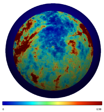
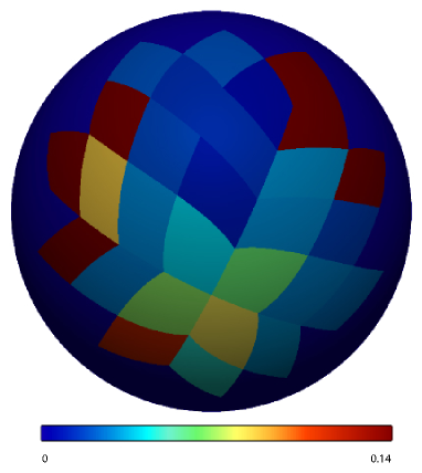
In order to estimate the PED amplitude in a given patch, we follow the prescription of Ref. Clark:2012sa . The PED angular power spectrum is assumed to obey a power law,

$$\frac{\ell(\ell+1)}{2\pi}C^{D}_{\ell}=A\ell^{m},$$ (1)

where the power-law index $m$ is fixed to its full-sky best-fit value $m=-0.22$ in this template, and $A$ is allowed to vary between different patches. To estimate $A_{p}$ for a given patch $p$, we calculate the variances $\sigma_{Q}^{2}=\langle Q^{2}\rangle_{p}-\langle Q\rangle_{p}^{2}$ and $\sigma_{U}^{2}=\langle U^{2}\rangle_{p}-\langle U\rangle_{p}^{2}$ of the polarization in both the $Q$ and $U$ components of the patch, and infer a power-spectrum amplitude from each, using the relation

$$\sigma^{2}=\frac{1}{4\pi}\sum_{\ell=2}^{\ell_{\rm max}}(2\ell+1)C^{D}_{\ell}B^{2}_{\ell}(\theta_{s}).$$ (2)

We then take the average of the resulting amplitudes to be the PED B-mode power-spectrum amplitude in the desired patch, under the assumption that power is equally distributed between the E and B modes.

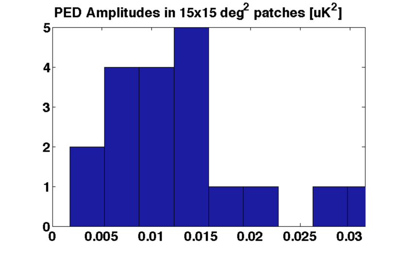
Finally, to remain with a realistic set of possible patches, we immediately apply a cutoff to remove the noisiest patches from our sample. The choice of cutoff represents prior knowledge regarding the expected PED amplitudes in this region given the templates and results of previous surveys. We choose a cutoff of $33\%$ throughout. A histogram of PED amplitudes $A_{p}$ in the remaining $19$ patches within the region shown in Fig. 1 is plotted in Fig. 2, with a normalization of $3.6\%$. We see that the amplitudes in this sample still vary over more than an order of magnitude.

Figure 2: A histogram of dust amplitudes $A_{p}$ in $19$ patches of $15^{\circ}\times 15^{\circ}$ within the region plotted in Fig. 1, calculated using Eq. (2), after a cutoff at the $67$th-percentile to remove the noisiest patches from our sample altogether.

Before moving on to survey optimization methods, we wish to examine the expected signal, noise and foreground amplitudes. We defer the instrumental noise calculation (as well as the statistical estimators used to measure CMB power spectra) to the Appendix, and present the results here.

We consider three types of fiducial experiments whose parameters are given in Table 1. Experiment 1 is inspired by the POLARBEAR experiment POLARBEAR and observes a single $15^{\circ}\times 15^{\circ}$ patch. Experiment 2 has similar properties, but a smaller sky coverage, optimized for detecting the peak of the primordial B-mode power spectrum at $\ell\sim 10^{2}$ (without de-lensing, the optimal size may be a bit larger Kesden:2002ku ). Experiment 3 is a fiducial lower-cost, lower-resolution experiment targeted at the larger scale primordial B-mode signal (hence the larger sky coverage). We assume an observing efficiency of $20\%$ for all three experiments.

Experiment	$\theta_{\rm fwhm}$	$f_{\rm sky}$	$T$	$s$=NETarray
	[arcmin]	[%]	[years]	[$\mu{\rm K}\sqrt{\rm sec}$]
1	3.5	0.55	2	$\frac{480\sqrt{2}}{\sqrt{1274}}=19$
2	5	0.014	2	15
3	30	1.52	6	25

Table 1: Parameters for three CMB polarization experiments we use for our analysis. Here, $s$ is the single-detector polarization sensitivity divided by the square root of the number of detectors.

In Fig. 3, we plot the expected noise power spectrum of our fiducial experiments, together with the primordial B-mode power spectrum for tensor-to-scalar ratios $r=0.05,\,0.01$. The lensing contribution to the B-mode signal is plotted separately. We also plot the PED power spectra for the maximum-, median-, and minimum-amplitude patches in our sample, for two fiducial normalization levels, corresponding to the values $3.6\%$ and $10\%$ of average dust polarization fraction outside the Galactic plane.

Figure 3: A plot of the relevant power spectra: the primordial B modes for $r=0.05$ and $r=0.01$ (in solid and dashed cyan), the lensing-induced B-mode contribution (magenta), the instrumental noise for our three fiducial experiments (gray dashed, dot-dashed and solid lines)—each limited to a different $\ell$ range (shaded gray regions)—and the maximum, median, and minimum PED power spectra in $19$ non-overlapping $15^{\circ}\times 15^{\circ}$ patches, for $3.6\%$ (solid) and $10\%$ (dashed) normalization values (in blue, red and green).

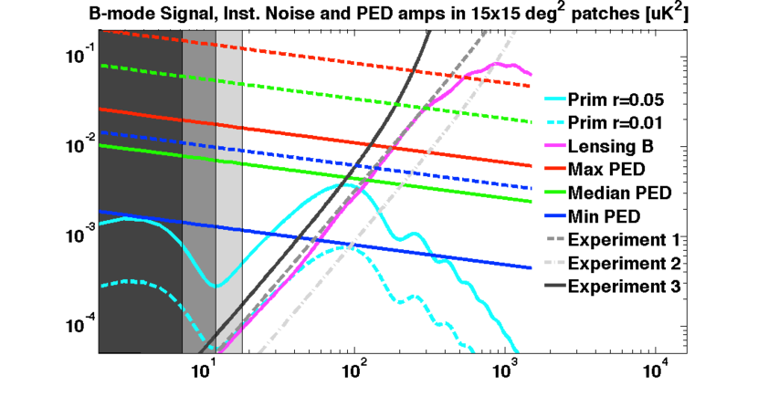
We can see that the primordial contribution to the signal peaks once at very low $\ell$ (due to the reionization contribution) and then again around $\ell\sim 10^{2}$, while B modes from lensing become dominant at smaller scales and peak around $\ell\sim 10^{3}$. At low $\ell$, the signal lies below most fiducial noise levels, except perhaps the optimal patches of sky under the assumption that the average dust polarization fraction is not too high. Therefore, it is clear that foregrounds pose a serious challenge to a single-frequency measurement, and a systematic method to identify lower-noise patches may be useful.

III Exploration vs. Exploitation

We now describe the methodology for constructing adaptive survey strategies to identify the optimal patches within an initial set of candidates. Using consecutive short-time measurements of B modes over the patches, we will show how heuristic machine-learning algorithms can be used to converge onto the optimal patch.

III.1 Constructing and Evaluating Adaptive Strategies

A strategy to find the best patch uses a set of estimates for the expected rewards of each patch in order to decide which one to select at each step. The expected (or mean) reward of each patch $patch$ is called its action-value, and we denote it by $\mu^{*}(p)$. We define $V_{i}$, the reward of the each of these short measurements, as $V_{i}=-\widehat{A_{p}}_{i}$, where $\widehat{A_{p}}_{i}$ is the estimated dust-amplitude in patch $p$ from measurement $i$. The goal of the survey strategy will thus be to identify the patch with the highest true reward $\mu^{*}(p)$

A natural way to estimate the action-value of a patch after $t$ steps is through sample-averaging of its previous rewards. If at step $t$ a patch $p$ has been chosen $N_{t}(p)$ times and has yielded a set of rewards $V_{1},V_{2},\dots,V_{N_{t}(p)}$, then its action-value estimate will be given by

$$\mu_{t}(p)=\frac{\mu_{0}(p)+V_{1}+V_{2}+\dots+V_{N_{t}(p)}}{N_{t}(p)+1},$$ (3)

where the values $\mu_{0}(p)$ are defined by some chosen method of initialization. The law of large numbers then guarantees that $\mu_{t}(p)\to\mu^{*}(p)$ as $N_{t}(p)\to\infty$.

The standard figure of merit for the success of a proposed algorithm to solve a problem of this type is its total regret. if $V^{*}=\underset{p}{\operatorname{max}}\,\mu^{*}(p)$ is the expected reward of the optimal patch $p^{*}$, then after $t$ plays the total regret is given by

$$R_{t}=\left\langle\sum\limits_{t=1}^{T}\left[V^{*}-\mu_{t}(p)\right]\right\rangle=\sum\limits_{p}\left\langle N_{t}(p)\right\rangle\Delta_{p},$$ (4)

where $\Delta_{p}=V^{*}-\mu^{*}(p)$ is the gap between the optimal reward and the expected reward of patch $p$. Therefore, a good strategy ensures smaller counts for larger gaps.

The performance of any strategy depends on the similarity between the optimal patch and the other patches. The hardest problems will have similar-looking patches with slightly different means. In the context of MAB solutions, Lai and Robbins LaiRobbins have derived a lower bound for the asymptotic total regret in the limit of unlimited number of plays. As we demonstrate below, this bound applies quite well to the algorithms we consider below for B mode survey strategies as well. According to their theorem,

$$\lim_{t\to\infty}R_{t}\geq\log{t}\sum\limits_{p|\Delta_{p}>0}\frac{\Delta_{p}}{KL(\mathcal{P}(p)||\mathcal{P}(p^{*}))},$$ (5)

where $KL(\mathcal{P}(p)||\mathcal{P}(p^{*}))$ is the Kullback-Leibler (KL) distance KLdiv between the probability distributions of a patch $p$ and the optimal patch $p^{*}$. If the rewards have normal distributions, $\mathcal{N}(\mu^{*}(p),\sigma_{p})$ and $\mathcal{N}(\mu^{*}(p^{*}),\sigma_{p^{*}})$, the KL distance between two patches is given by Kullback

$$KL(\mathcal{P}(p)||\mathcal{P}(p^{*}))=\ln{\frac{\sigma_{p^{*}}}{\sigma_{p}}}+\frac{\sigma^{2}_{p}+\left(\mu^{*}(p^{*})-\mu^{*}(p)\right)^{2}}{2\sigma_{p^{*}}^{2}}-\frac{1}{2}$$ (6)

In practice, achieving logarithmic total regret is a challenge, requiring an ideal tradeoff between exploration and exploitation. It is easy to see from Eq. (4) that an algorithm that never explores will have linear total regret and the same is true for an algorithm that explores forever.

III.2 Families of Heuristic Solution Methods

We briefly describe a set of algorithms that represent some of the prevailing heuristics in the literature to solve problems of this type.

• Greedy

  The most naive approach to this optimization problem is simply to select at each observation “step” $t$ the patch with the highest estimated action-value

  $$p_{t}=\underset{p}{\operatorname{argmax}}\,\mu_{t}(p).$$ (7)

  This method merely exploits past knowledge in order to maximize the immediate reward (hence greedy Cormen ) and results in linear total regret. In the absence of any initial knowledge regarding the expected rewards (setting all $\mu_{0}(p)=-M$ where M is very large), this method chooses one of the patches randomly on the first step and then continuously exploits it, without any further exploration.

• $\epsilon$-greedy

  A simple enhancement to the regular greedy method is to occasionally force the selection of a patch at random, regardless of the action-value estimates. In the $\epsilon$-greedy method, at probability $1-\epsilon$ the greedy patch is chosen, while at probability $\epsilon$ a patch $p$ (out of a total $n_{p}$ patches) is chosen uniformly at random. In the limit $\epsilon\to 0$, this reduces to the regular greedy method. When $\epsilon=1$, this method forever exploits all patches uniformly.

• Decaying $\epsilon$-greedy

  While perpetual exploration ensures the convergence of all the action-value estimators $\mu_{t}(p)\to\mu^{*}(p)$ (since $N_{t}(p)\to\infty$ for all patches), it also means that exploration continues even after the optimal patch is identified with great (and ever-growing) confidence. To solve this problem, a further enhancement to this method is to decrease the exploration probability $\epsilon$ with time. In practice, however, it is hard to choose a single decay strategy for $\epsilon$ that works well under different circumstances (different reward distributions).

• Optimistic initialization

  We implement the absence of prior knowledge by taking the limit $\mu_{0}(p)\to-\infty$ (we take $\mu_{0}(p)=-M$ where M is very large). Any other choice for the initial action-value estimates would introduce a bias in all the methods described so far, but an effective choice of this bias can be used as a means of forcing an early stage of increased exploration. For example, by choosing optimistically-high initial values in the greedy method, we delay the convergence onto a single patch until the initial values no longer dominate the sample average. Until that happens, some knowledge will have been gathered about all patches, ensuring a more informed greedy choice from then on, at the expense of this initial stage of exploration.

• Probability matching (Boltzmann)

  An obvious path towards more sophisticated algorithms is to vary the probability with which inferior patches are explored, instead of sampling them uniformly as in $\epsilon$-greedy. After all, $\epsilon$-greedy is likely to keep exploring extremely unfavorable patches even after they are known to be vastly inferior to others. The straightforward solution is to set the probability to explore each patch according to its estimated value. In the Boltzmann method (or Thompson sampling Thompson ), for example, the probability to choose patch $p$ at play $t$ is given by

  $$\text{Prob}_{t}(p)=\frac{e^{\mu_{t}(p)/\tau}}{\sum\limits_{p^{\prime}}e^{\mu_{t}(p^{\prime})/\tau}},$$ (8)

  where $\tau$ is a positive parameter, often referred to as the temperature. In the high-temperature limit, this reduces to the $\epsilon=1$ uniform method, while in the $\tau\to 0$ limit we retrieve the regular greedy method with absence of initial knowledge.

  Although some quantitative studies have been performed to compare the Boltzmann and $\epsilon$-greedy methods, no consistent conclusions as to which is superior have been reached Sutton ; McGill . Both methods depend on the tuning of their respective free parameter and one performs better than the other under different circumstances. We shall use the Boltzmann method with optimistic initialization, as our experience deems this favorable.

• Upper confidence bound

  The upper confidence bound (UCB) method Auer tackles the exploration-versus-exploitation tradeoff according to the principle that the more uncertain we are about the action-value of a patch, the more important it is to explore it further (since it could turn out to be the optimal one). In this method, we estimate an upper confidence $U_{t}(p)$ for each action value such that $\mu(p)\leq\mu_{t}(p)+U_{t}(p)$ with high probability, and then select the action that maximizes the sum $\mu_{t}(p)+U_{t}(p)$

  $$p_{t}=\underset{p}{\operatorname{argmax}}\left\{\mu_{t}(p)+U_{t}(p)\right\}.$$ (9)

  The confidence bound depends on the number of times $p$ has been selected (as increased selection reduces the uncertainty bound). When the rewards are Gaussian, a useful upper bound is given by $c\,\sigma_{p}/\sqrt{N_{t}(p)}$, where $c>0$ is some constant. As a prior for the upper bound is used in this method, it is often referred to as the “UCB Bayesian” method.

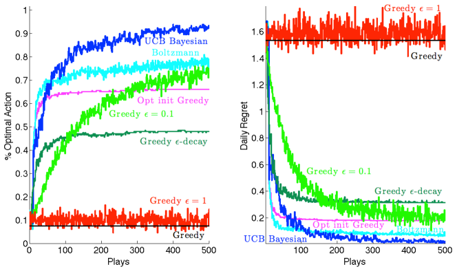
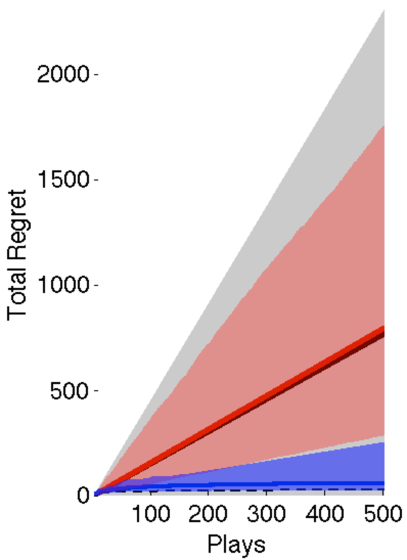
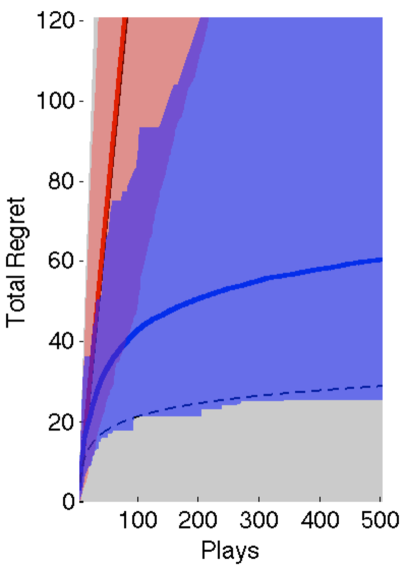
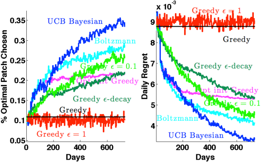
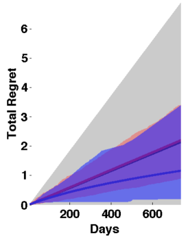
Before moving on to the implementation of these heuristic strategies in B-mode experiments, we demonstrate their performance for a simple problem with $10$ patches with reward distributions $\mathcal{N}(\mu^{*}_{p},1)$, where the mean rewards $\mu^{*}_{p}$ are themselves drawn from a normal distribution, $\mathcal{N}(0,1)$. In Fig. 4 we plot the behavior of each of the methods with time. Most methods converge onto the optimal patch in greater percentages and decrease their daily regret as time goes by. The UCB method seems more successful eventually than others, while the second-best Boltzmann method is the most efficient after a very limited number of plays. In Fig. 5 we compare the total regret for three algorithms: greedy, $\epsilon$-greedy with $\epsilon=1$, and UCB. We plot the average in solid lines and the full range of performance in the corresponding shaded regions. The greedy method will always have the widest range of performance, as it chooses and stays with the optimal patch or worst patch at $10\%$ probability. The UCB method has logarithmic total regret, much like the Lai and Robbins asymptotic bound, also plotted.

Figure 4: Different algorithms balance exploration and exploitation differently. Left: The percentage of simulations in which the optimal patch was chosen in each play. The UCB method reaches a higher percentage than all other methods as the number of plays is increased. Greedy and $\epsilon$-greedy with $\epsilon=1$ choose the optimal patch $10\%$ of the time, which is expected with a total of $10$ patches. Right: The average regret at each play. Notice that the Boltzmann method is inferior to UCB in the long run, but it reduces the daily regret faster than UCB at the beginning.

Figure 5: Left: The average and ranges of total regret for greedy (range: shaded gray, average: solid black), $\epsilon$-greedy with $\epsilon=1$ (red) and UCB (blue). Right: Zooming in $\rightarrow$ the UCB method assumes logarithmic behavior, similar to that of the Lai and Robbins asymptotic bound (in dashed-black), after a relatively small number of plays.

III.3 Testing a B-mode adaptive strategy

We now apply the heuristic adaptive-survey strategies discussed above to simulated CMB-polarization maps. As detailed below, each “step” will be a short-duration measurement of the polarization on one of $n_{p}$ patches of sky available to observe. It is assumed that the data from this short-duration experiment is analyzed under the null hypothesis of no gravitational waves ($r=0$) to obtain an estimate (albeit very rough) of the dust amplitude in that patch. The “reward” from that “pull” is then the dust amplitude inferred from that measurement multiplied by $-1$ (so that subsequent measurements are steered toward lower dust amplitudes). The chosen algorithm then uses whatever information it has collected from measurements done so far on dust amplitudes to decide which patch to observe next. At no point does the algorithm make use of any prior information about $A_{p}$, nor does it make any use of the error estimates in Eq. (14) for $r$.

In more detail, to test the adaptive strategies, we first simulate an observed sky as follows: We first apply an upper cutoff in amplitude to the desired-size patches in the South Pole region FGPol template to remain with a certain percentage of lowest-noise patches, representing our prior knowledge regarding the target area, either from the noise templates themselves or from other surveys. As mentioned above, for all experiments we limit our sample to patches with PED amplitudes below the $67$th percentile. We then randomly draw a subset of $n_{p}$ dust amplitudes from the truncated sample. These are drawn at the onset of each simulation and then kept fixed.

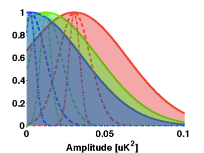
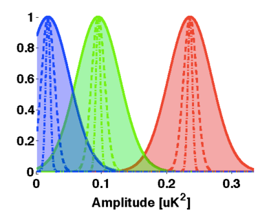
Meanwhile, we choose the time-step size, $t_{\rm step}$, typically a few observation days. We also use the fiducial experimental parameters in Table 1 to set the parameters $s$, $T$, $f_{\rm sky}$, and $\sigma_{b}$. We then use Eq. (13) to calculate the “1-sigma” error $\sigma^{\widehat{A}}$ with which the chosen experiment can measure the dust amplitude of a patch in a single time step. (This $\sigma^{\widehat{A}}$ corresponds to the width of the likelihood functions in Fig. 8).

Finally, we apply the strategies to the simulated sky to allocate the amount of time spent on each patch. At each time step $i$, we do the following:

• Choose which patch to observe according to the strategy we employ.

• Retrieve a reward $V$ for this patch for this time step through a random draw from a normal distribution, $V=-{\rm max}(0,\mathcal{N}(A_{p},\sigma^{\widehat{A}}))$. The minus sign is chosen so that the methods converge onto lower-noise patches.

• Update our action-value estimate $\mu_{t}(p)$ of the chosen patch $p$ according to the reward.

• Decide which patch to observe at the next time step according to the strategy or stop the simulation if the total observation time has been exhausted. This decision is based solely on the averages we have, at this step, of draws from the $\widehat{A_{p}}$ maximum likelihood distribution.

• Calculate the regret, measured by the difference in the noise amplitude between the chosen patch and the lowest-noise patch and update the total regret. We also calculate the overall figure-of-merit (the smallest detectable tensor-to-scalar ratio at “1-sigma”) at each time $T^{i}$ by plugging in the total observation times spent so far on each patch $t^{i}_{p}$ (where $\sum\limits_{p=1}^{n_{p}}t^{i}_{p}=T^{i}$) and the (known) dust amplitudes $A_{p}$ into Eq. (15). The regret and the overall figure-of-merit are calculated but never used during the experiment. They are calculated only to allow us to evaluate at the end of the experiment how well the strategy has converged to the cleanest patch of sky and how well it has improved the smallest B-mode amplitude $r$ that can be distinguished from a null result.

Our choice of parameters for the different methods:

• In the absence of initial knowledge: $\mu_{0}(p)=-3\sigma^{\widehat{A}}$

• For $\epsilon$-greedy, we choose $\epsilon=0.1$.

• Our $\epsilon$-decay strategy is $\epsilon={\rm min}(1,n_{p}\sigma^{\widehat{A}}/\sqrt{t})$.

• For Optimistic Initialization: $\mu_{0}(p)=3\sigma^{\widehat{A}}$.

• For the Boltzmann method, we choose $\tau=0.001$.

• For UCB we take $c=1/2$: $U_{t}(p)=\sigma^{\widehat{A}}/2\sqrt{N_{t}(p)}$.

We then repeat the full list of steps above $1,000$ times in order to acquire an ensemble of simulations for comparison. We thus explore the improvement in the upper bound on the tensor amplitude $r$ obtained with one strategy to that obtained with another strategy. What changes between the simulations is the set of dust amplitudes $A_{p}$ that we draw each time from the FGPol template, as well as the random choices made by some of the algorithms. In the next Section we study the performance of each of the strategies above for our fiducial experiments (see Table 1) and for the best-, conservative- and worst-case scenarios regarding the PED normalization.

IV Results

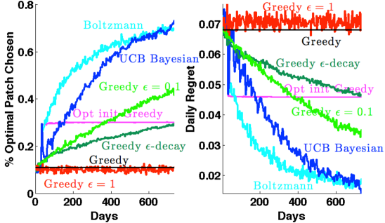
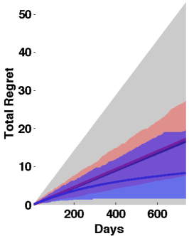
We are now ready to test our strategies on simulations of B-mode experiments. We first address the extreme cases (see Fig. 8) of $10\%$ average dust polarization fraction with no-delensing (a pessimistic scenario) and $3.6\%$ with an efficient de-lensing process, leaving only a $20\%$ residual (an optimistic scenario). Focusing on Experiment 1, which has properties similar to the POLARBEAR experiment POLARBEAR , we compare the performance of the different strategies in Fig. 6 using our simulations. We see that the UCB method fares better than other methods in identifying the optimal patch, although it does not achieve the same rate of success as in our simple Gaussian test case above. With a distribution of foreground amplitudes taken from the FGPol templates in the region of Fig. 1, after a cutoff at the $67$th percentile, the UCB method manages to converge onto the optimal patch after 2 years of observation in only $\sim 80\%$ of the simulations in the pessimistic scenario and in less than half of the simulations in the optimistic one. Nevertheless, we see that the total regret in the optimal methods (Boltzmann, UCB) is much lower than with naive methods. The total regret in the greedy method, which is the default version of a POLARBEAR-type experiment, is roughly 2–3 times higher when comparing the average or worst-case performance to those of UCB. Greedy with $\epsilon=1$, which corresponds to an SPT-type experiment, where a larger region is uniformly observed (or several patches uniformly integrated over), is better in the worst case than greedy, but also never reaches below the average of the UCB method in the pessimistic scenario (and barely below the average of UCB in the optimistic scenario), even in its best-case performance.

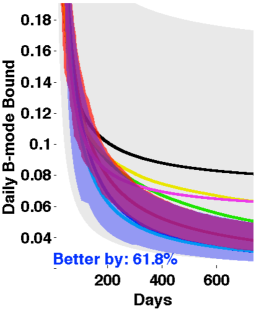
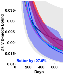
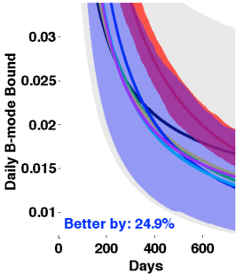
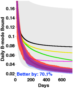
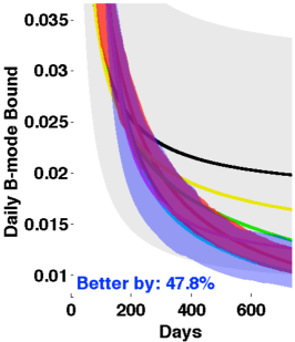
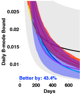
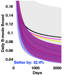
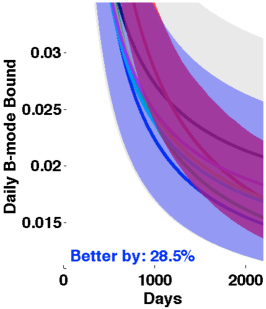
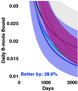
As we explained above, our overall figure-of-merit in comparing adaptive survey strategies is the smallest detectable tensor-to-scalar ratio $r$ at “1-sigma” confidence. In Fig. 7, we plot our results for the three experiments in Table 1, for three scenarios: a pessimistic scenario with $10\%$ dust polarization fraction and no de-lensing, a conservative scenario with $3.6\%$ normalization and no de-lensing and an optimistic scenario with $3.6\%$ normalization and a $20\%$ lensing residual. In all cases, the UCB method achieves the best results for all experiments (though it is very close to the Boltzmann method in many instances). In the case of experiment 2 in the conservative scenario, even the best-case performance of the greedy method is inferior to the averages of the UCB method (and also $\epsilon$-greedy with $\epsilon=1$). This is because with this low-noise experiment, prolonging the integration, even over the cleanest patch, only goes so far and it is often preferable to spend equal time on the two (or more) cleanest patches.

We see that the improvement on average when comparing to the greedy method ranges from $\sim 25\%$ to $\sim 70\%$ (and it goes without saying that it will only improve further if the observation is prolonged). Thus, adaptive strategies have great potential to improve the sensitivity in IGW searches.

Figure 6: The percentage of $1000$ simulations in which the optimal patch was chosen per day (left), the average daily regret (center) and the average total regret (right) for Experiment 1. Top Row: A pessimistic scenario of no-delensing and $10\%$ average dust polarization fraction. Bottom Row: The optimistic case of $3.6\%$ normalization and $80\%$ de-lensing. We see that the UCB method ultimately chooses the optimal patch in larger percentages compared to other methods (although the Boltzmann method ramps up its performance more quickly at the onset). The UCB method achieves the lowest total regret on average, and even in its worst case (top of shaded-blue region), it is relatively close to the averages of greedy (black line, almost overlapping the red line, with gray shading) and $\epsilon$-greedy with $\epsilon=1$ (red), whose own worst cases are roughly 4 and 10 times the UCB average.

Figure 7: The average smallest detectable tensor-to-scalar ratio with different adaptive survey (bandit) strategies. The greedy method is drawn in black, with its best and worst performances bracketing the area shaded in gray. Greedy with $\epsilon=1$ is drawn in red and its performance interval is also shaded in red. The best-performing method in all scenarios is UCB and its performance range is shaded in blue. We also note the best improvement achieved with respect to greedy. Column 1 is for the worst-case $10\%$ normalization scenario, Column 2 is for the conservative scenario of $3.6\%$ normalization and Column 3 is for the optimistic case of $3.6\%$ normalization and $80\%$ de-lensing ($\alpha=0.2$ in Eq. (15)). Top Row: Experiment 1, with $n_{p}=10$ patches and step-size of three observation days. Middle Row: Experiment 2, with $n_{p}=15$ patches and step-size of six observation days. Bottom Row: Experiment 3, $n_{p}=5$ and the step-size is three days.

V Discussion

V.1 Simplifying assumptions and caveats

It is worthwhile to discuss several simplifications we have made throughout the analysis above. First, we have made exclusive use of the FGPol templates O'Dea:2011kx both to motivate the need for adaptive survey strategies and in order to estimate the expected distribution of foreground levels across the sky. The use of other templates that have been developed in the literature Schlegel:1997yv ; Fantaye:2011zq ; Delabrouille:2012ye , or the recent high-frequency polarization measurements by the Planck experiment (which are not sensitive enough to efficiently constrain the polarization dust amplitudes in low intensity regions), may lead to somewhat different results, but most likely will not alter our conclusions. In the future, as better data is accumulated, it will be worthwhile to consider improvements upon the methods presented above. For example, one way to incorporate prior data is in the initialization of the different action-value estimates of the targeted patches, which will ensure faster convergence onto optimal patches.

Secondly, we have limited our analysis to the case of experiments operating at a single frequency. This allowed us to focus on a single source of foregrounds and work under the assumption that it could not be efficiently removed through component separation or other methods. Most B-mode experiments will eventually gather measurements from multiple frequencies in order to enable foreground subtraction. In this case, the foreground amplitudes we have considered here will be replaced by the amplitude of the remaining residuals KovKamExploration . In a very optimistic scenario, where these would be smaller than the IGW B-mode signal, the advantage of our methods would be restricted. In KovKamExploration , we elaborate on this issue and present a different approach, whereby an independent stage of exploration at higher-frequencies is performed before the stage of prolonged observation.

Additional assumptions include the neglect of E and B mode mixing, which may pose a problem in partial sky measurements Amblard:2006ef ; Bunn:2002rx ; Zhao:2010sza (although optimized estimators greatly reduce this complication Smith:2005gi ) and the approximation that the likelihood curves for the power spectra estimators are Gaussian (in our B-mode simulations we simply drew a measured amplitude from a normalized distribution matching the likelihood mean and width, as opposed to drawing the estimated value for each multipole from a corresponding $\chi^{2}$ distribution). We do not expect these assumptions to have a meaningful impact on our results.

Finally, we have limited our analysis to just a handful of scenarios, ranging from pessimistic to optimistic, in an attempt to provide a complete picture regarding the prospects of the methods proposed. We have verified that changing some of the parameters chosen here, such as the power-law index for the PED power spectrum, the level of dust polarization fraction outside the Galactic plane and the efficiency of the de-lensing process, do not substantially affect our conclusions. However, a more detailed study should be conducted when implementing these methods to a specific B-mode experiment. One enhancement upon our analysis is to calculate the full foreground power spectrum directly from the template patch, instead of relying on a best-fit power law. Another important ingredient to include is the cost of moving between different sky patches when calculating the total regret of different observing strategies. While this may degrade the improvement in sensitivity somewhat, it will be offset by the continued gain from identifying the optimal patches for observation as the experiments progress to their next stages, which we have not taken into account here.

V.2 Adaptive strategies elsewhere

Analogous adaptive survey strategies might also be used to help detect 21-cm intensity fluctuations from the EoR Furlanetto ; Morales , where the signal must be distinguished, using angular and/or frequency information, from a variety of Galactic and extragalactic foregrounds Jelic:2008jg ; Dimatteo:2001gg ; Oh:2003jy ; Santos:2004ju ; Bowman:2008mk ; Liu:2011hh ; Gleser:2007fg that are expected to be larger by several orders of magnitude. The desired signal is expected to extend from several arcminutes to several degrees. What is currently envisioned, for example, for the Low Frequency Array LOFAR and the Square Kilometer Array SKA , is a deep integration on a $\sim 5^{\circ}\times 5^{\circ}$ region of the sky. As is well known by now, the amplitude of Galactic foregrounds may vary considerably from one such region on the sky to another. While existing Galactic dust and synchrotron maps can be used to identify regions of the sky that are likely to be clean, again, detailed maps at the several-hundred MHz frequencies of interest, with the angular resolutions of interest, do not exist. There are also likely to be foregrounds in frequency space contributed by radio recombination lines Oh:2003jy , and little is known about their distribution at the high Galactic latitudes that present the likeliest targets for these deep EoR integrations. The distribution of the extragalactic-foreground intensity across the sky is expected to be smoother than the Galactic foregrounds. Even so, clustering of highly-biased radio sources at high redshift may give rise to significant variation in foreground intensities from one patch of the sky to another. The aim of an adaptive bandit strategy would in this case be to identify the cleanest patch in a fixed survey time.

Another example of a foreground-limited stochastic measurement is that of a gravitational wave background (GWB) PrimGWBack1 ; PrimGWBack2 , which may be pursued by terrestrial experiments such as The Laser Interferometer Gravitational Wave Observatory LIGO and several Pulsar Timing Array consortia IPTA . In the relevant frequency bands, the stochastic GWB signal may be obscured by confusion foreground stemming from bright sources, including supermassive black hole binaries Jenet:2006sv , neutron star binaries Regimbau:2005ey and Galactic white dwarf binaries Evans . In an effort to minimize the effect of foregrounds, adaptive strategies may be used to improve the sensitivity of the relevant ground-based experiments.

Likewise, similar strategies should be explored for a JWST deep field aimed to detect the first stars/galaxies Bromm:2003vv ; Barkana:2000fd . CMB measurements of the reionization optical depth suggest that the first stars formed at redshfits $z\sim 10$, and these stars should emit radiation that today falls in the wavelengths probed by JWST Santos:2002hd ; Trenti:2009cj . Still, the abundance of these objects, their luminosity function, etc., are largely a matter of guesswork. It may well be that the population of the first stars/galaxies will fill the entire image, or that there may be a vast population of low-flux sources from lower redshifts that may obscure the EoR objects of interest, as suggested in Ref. Windhorst:2007 . The very faint EoR sources, in this case, will be easiest identified in the cleanest field on the sky. Again, an adaptive survey strategy to identify the cleanest of several candidate patches may well be warranted.

In this regard, one should be mindful of an inherent difference between the application of adaptive survey strategies to stochastic measurements and deep-field imaging. While a choice of an optimal sky patch for deep-field imaging may considerably improve the sensitivity of a given experiment, the initial stage of exploration is mostly wasted. Therefore, the overall figure-of-merit when comparing different strategies should be the speed of convergence onto the optimal patch instead of the total regret, and the best-performing algorithms may be different. Nevertheless, an initial stage of exploration may still prove invaluable in reducing the error in the integrated signal from the chosen patch to image.

A somewhat different kind of MAB-like problem in the context of astronomical observations shows up in the case of follow-up observations of transients Djorgovski:2011rv , for example. In this case, the exploration versus exploitation tradeoff is manifested in the challenge of allocating the wide array of resources to the task, each with very different characteristics and cost functions. Hence, the overall figure-of-merit for comparing various algorithms may once again be different than considered here.

We leave the detailed study of the prospects of adaptive strategies in these setups to future work.

VI Conclusion

The era of CMB B-mode measurements has only just begun Zaldarriaga:1998ar ; SPTpolBModes ; Ade:2014afa ; Ade:2014xna . The race for the detection of IGW B modes is picking up and the competing efforts will be mainly characterized by their ability to tighten the upper bound on the tensor-to-scalar ratio. This endeavor is extremely difficult and will grow more so as the upper bound is decreased, particularly due to the major obstacles which need to be efficiently removed — foreground contamination and lensed E modes — whose amplitudes are independent of the targeted IGW B-modes. Therefore, any novelty in the approach to conducting these measurements which may mitigate these problems is both timely and important.

In this paper we have proposed exactly such a novelty, in the form of adaptive survey (bandit) strategies, inspired by heuristic solutions to the MAB problem. Focusing on polarized foreground components, whose amplitudes are predicted to vary considerably across the sky, our target was to balance the time spent on exploration to find lower-noise patches of sky with that devoted to exploitation of the optimal patches through deep integration. By formulating this tradeoff as a machine-learning problem, we were able to adopt heuristic algorithms developed in the general context of the MAB challenge and implement them in the settings of fiducial B-mode experiments.

Attempting to go beyond a mere proof-of-concept, we have incorporated a number of crucial ingredients into our analysis, such as prior knowledge from existing surveys, several fiducial sets of instrumental properties, different possible forecasts regarding the average amplitude of foregrounds, and realistic prospects for the level of lensing residuals (including pessimistic cases of no de-lensing). Relying on advanced templates for polarized emission from dust in the Galaxy, we demonstrated that single frequency experiments could improve their upper bounds on the tensor-to-scalar ratio by factors of a few on average and even higher when comparing worst-case performances of standard methods versus the ones proposed here.

The assumptions made in this work were discussed in the previous section, along with some possible caveats in the implementation of the adaptive survey strategies proposed here in B-mode experiments. While the precise improvement these methods may enable remains to be seen, we feel that the case has been made for their consideration in any ground-based experimental setup focusing on CMB B-mode detection with partial sky coverage.

Lastly, as the tradeoff between exploration and exploitation shows up in other realms of observational cosmology as well, this work opens the door for additional applications of adaptive survey strategies. These may include other stochastic measurements, such as the power spectrum of 21-cm fluctuations Furlanetto ; Morales ; Pritchard or a primordial GWB PrimGWBack1 ; PrimGWBack2 , deep-field imaging by radio interferometers LOFAR ; SKA or optical telescopes Windhorst:2005as ; Stiavelli , and the allocation of limited resources in follow-ups of identified astrophysical transients Djorgovski:2011rv , to name a few.

Appendix A B Mode Measurements

A.1 Instrumental Noise

The instrumental noise in a CMB-polarization experiment is determined by the detector-array sensitivity (or noise-equivalent temperature NET) $s$, its angular resolution $\theta_{\rm fwhm}$, the sky coverage $f_{\rm sky}$ and the total observation time $T$ (which is reduced in practice by the observing efficiency). The pixel noise $\sigma_{\rm pix}=s/\sqrt{t_{\rm pix}}$ is determined by the detector sensitivity $s$ and the observation time $t_{\rm pix}=T/N_{\rm pix}$ dedicated to each pixel. Defining the inverse weight per solid angle, $w^{-1}(T)=4\pi s^{2}/T$, the angular power spectrum of the instrumental noise, assuming the experimental beam is approximately Gaussian in shape, is given by Tegmark:1997vs

$$C^{N}_{\ell}=\frac{\Omega\sigma_{\rm pix}^{2}}{N_{\rm pix}}e^{\ell^{2}\sigma_{b}^{2}}=\frac{\Omega s^{2}}{T}e^{\ell^{2}\sigma_{b}^{2}}=f_{\rm sky}w^{-1}(T)e^{\ell^{2}\sigma_{b}^{2}},$$ (10)

where $\Omega=4\pi f_{\rm sky}$ and $\sigma^{2}_{b}=\theta^{2}_{\rm fwhm}/(8\ln{2})$.

A.2 Statistical Estimators on Partial Sky

The measurements we deal with are those of power spectra. In a maximum-likelihood analysis, the Fisher forecast for the error in the measurement of the amplitude $A$ of a power spectrum $C_{\ell}$ is given by Jaffe:2000yt ,

$$\frac{1}{\sigma_{A}^{2}}=\sum_{\ell}\left(\frac{\partial C_{\ell}}{\partial A}\right)^{2}\frac{1}{\sigma_{\ell}^{2}}.$$ (11)

We will work under the assumption that the likelihood function is Gaussian in the vicinity of its maximum Jungman:1995bz ; Zhao:2008re . To emphasize this approximation we use quotation marks around “1-sigma” when referring to the error $\sigma_{A}$.

In order to choose between exploration and exploitation on the fly, we need to estimate the PED amplitude $A$ in a targeted patch within the observation time allotted to a single step of the experiment. For a given sky coverage $f_{\rm sky}$, the “1-sigma” error for an individual $\ell$ in the estimated value $\widehat{A}$ is Jaffe:2000yt ; Knox:2002pe ; Kesden:2002ku

$$\sigma_{\ell}^{\widehat{A}}=\sqrt{\frac{2}{f_{\rm sky}(2\ell+1)}}\left(\alpha C^{L}_{\ell}+f_{\rm sky}w^{-1}(t_{\rm step})e^{\ell^{2}\sigma_{b}^{2}}\right),$$ (12)

where $C^{L}_{\ell}$ is the lensing B-mode contribution and $w^{-1}(t_{\rm step})$ is the inverse weight per solid angle given $t_{\rm step}$ observation time. The quantity $1-\alpha$ parametrizes the level of de-lensing Sigurdson:2005cp ; Smith:2010gu that was applied to the data. When comparing forecasts for upper bounds on the tensor-to-scalar ratio, we will consider $\alpha=0.2$ and $\alpha=1$ as best and worst-case scenarios, respectively. The total “1-sigma” error in the measurement of $\widehat{A}$ over a time $t_{\rm step}$ is thus,

$$\sigma^{\widehat{A}}=\left[\frac{f_{\rm sky}}{2}\sum\limits_{\ell_{\rm min}}^{\ell_{\rm max}}\frac{(2\ell+1)(\tilde{C}^{D}_{\ell})^{2}}{\left(\alpha C^{L}_{\ell}+f_{\rm sky}w^{-1}(t_{\rm step})e^{\ell^{2}\sigma_{b}^{2}}\right)^{2}}\right]^{-\frac{1}{2}},$$ (13)

where $\tilde{C}_{\ell}^{D}=C^{D}_{\ell}/A=2\pi\ell^{-m}/[\ell(\ell+1)]$ encodes the $\ell$ dependence of the PED power spectrum and $\ell_{\rm min}=180/\theta$ is the largest scale accessible by an experiment with sky coverage $f_{\rm sky}=\theta^{2}$.

In Fig. 8 we plot the normalized (Gaussian) likelihood curves for the measured amplitudes of the patches with maximum, median, and minimum PED amplitudes in the FGPol template (see Fig. 3). The goal of the adaptive survey (bandit) strategies will be to distinguish between the means of these distributions in order to spend more time observing lower-noise patches. Clearly, this task is harder when the similarity between the distributions is larger (we will quantify this in the next Section).

Figure 8: Left: Likelihood functions for the measured amplitude values for the maximum-, median-, and minimum-amplitude patches (in blue, red and green) from our sample of $19$ non-overlapping $15^{\circ}\times 15^{\circ}$ PED patches in the conservative scenario of $3.6\%$ average dust polarization fraction, given the instrumental noise of Experiment 1. Widths correspond to step sizes of 3, 10 and 30 days of observation (in solid, dashed and dot-dashed, respectively). Right: Same plots for the worst-case $10\%$ average dust polarization fraction, in which case it is much easier to discern between the patches.

Our figure of merit when comparing the prospects of different adaptive survey strategies will be the smallest amplitude of primordial B modes that can be distinguished from the null hypothesis at “1-sigma” confidence after a fixed total observation time $T$. Denoting the $\ell$ dependence of the IGW B-mode power spectrum by $\tilde{C}^{B}_{\ell}$, the smallest amplitude in a patch $p$ detectable at “1-sigma” (with a total $t_{p}$ observation time spent on that patch), according to Eq. (11), is then

$$\sigma_{p}^{r}=\left[\frac{f_{\rm sky}}{2}\sum\limits_{\ell_{\rm min}}^{\ell_{\rm max}}\left(\frac{\sqrt{(2\ell+1)}\tilde{C}^{B}_{\ell}}{A_{p}\tilde{C}^{D}_{\ell}+\alpha C^{L}_{\ell}+f_{\rm sky}w(t_{p})^{-1}e^{\ell^{2}\sigma_{b}^{2}}}\right)^{2}\right]^{-\frac{1}{2}}$$ (14)

Notice that we set the sample variance of the primordial signal to zero in this expression (since we are comparing to the null hypothesis).

Finally, if an adaptive survey ends up spending a different observing time $t_{p}$ (where $\sum\limits_{p=1}^{n_{p}}t_{p}=T$) on each of $n_{p}$ patches with known dust amplitudes $A_{p}={A_{1},\dots,A_{n_{p}}}$, then the smallest detectable primordial B-mode amplitude will be

$$\sigma^{\rm r}=\left[\frac{f_{\rm sky}}{2}\sum\limits_{p=1}^{n_{p}}\sum\limits_{\ell_{\rm min}}^{\ell_{\rm max}}\left(\frac{\sqrt{(2\ell+1)}\tilde{C}^{B}_{\ell}}{A_{p}\tilde{C}^{D}_{\ell}+\alpha C^{L}_{\ell}+f_{\rm sky}w(t_{p})^{-1}e^{\ell^{2}\sigma_{b}^{2}}}\right)^{2}\right]^{-\frac{1}{2}}$$ (15)

As we clarify above, this expression for $\sigma^{\rm r}$ is never used during the experiment by the algorithm employed to determine the allocation of time to different patches. We calculate it only after the experiment has ended and the total observation time has been allocated by the different adaptive strategies as an overall figure-of-merit to estimate how well the strategies have done in improving the sensitivity to $r$. As we furthermore clarify below, the adaptive (bandit) algorithms never assume any prior knowledge of the $A_{p}$s. All information with which decisions are made about time allocations come from the measurements themselves.

References

- (1) H. Robbins, Bull. Am. Math. Soc. 58, 527 (1952)
- (2) D. A. Berry and B. Fristedt, Bandit Problems: Sequential Allocation of Experiments (Chapman & Hall, London, 1985).
- (3) W. H. Press, talk at “Astrophysics At The Extreme , The Hebrew University of Jerusalem, Israel, December 2009, http://tsvi.phys.huji.ac.il
- (4) W. H. Press, Proc. Nat. Acad. Sci., 106 52, 22387 (2009).
- (5) T. L. Lai and H. Robbins, Advances in Applied Mathematics 6,4 (1985).
- (6) R. S. Sutton and A. G. Barton, Reinforcement Learning: An Introduction (MIT Press, Cambridge, 1998).
- (7) V. Kuleshov and D. Precup, sub. to J. of Mach. Learn. Res. , http://www.cs.mcgill.ca/ vkules/bandits.pdf
- (8) J. Gittins, K. Glazebrook and R. Weber, Multi-Armed Bandit Allocation Indices (Wiley, New York City, 2011).
- (9) M. Kamionkowski, A. Kosowsky and A. Stebbins, Phys. Rev. Lett. 78, 2058 (1997) [arXiv:astro-ph/9609132].
- (10) U. Seljak and M. Zaldarriaga, Phys. Rev. Lett. 78, 2054 (1997) [arXiv:astro-ph/9609169].
- (11) M. Kamionkowski and A. Kosowsky, Ann. Rev. Nucl. Part. Sci. 49, 77 (1999) [arXiv:astro-ph/9904108].
- (12) Z. Kermish, P. Ade, A. Anthony, K. Arnold, K. Arnold, D. Barron, D. Boettger and J. Borrill et al., arXiv:1210.7768 [astro-ph.IM].
- (13) B. G. Keating, P. A. R. Ade. J. J. Bock, E. Hivon, W. L. Holzapfel et al., Proc. SPIE 4843, Polarimetry in Astronomy, 284 (2003); [doi:10.1117/12.459274].
- (14) C. Bischoff et al. [QUIET Collaboration], [arXiv:1207.5562 [astro-ph.IM]].
- (15) C. D. Sheehy, P. A. R. Ade, R. W. Aikin, M. Amiri, S. Benton, C. Bischoff, J. J. Bock and J. A. Bonetti et al., arXiv:1104.5516 [astro-ph.IM].
- (16) P. Ade et al. [QUaD Collaboration], Astrophys. J. 674, 22 (2008) [arXiv:0705.2359 [astro-ph]].
- (17) J. E. Austermann, K. A. Aird, J. A. Beall, D. Becker, A. Bender, B. A. Benson, L. E. Bleem and J. Britton et al., Proc. SPIE Int. Soc. Opt. Eng. 8452, 84520E (2012) [arXiv:1210.4970 [astro-ph.IM]].
- (18) M. D. Niemack, P. A. R. Ade, J. Aguirre, F. Barrientos, J. A. Beall, J. R. Bond, J. Britton and H. M. Cho et al., Proc. SPIE Int. Soc. Opt. Eng. 7741, 77411S (2010) [arXiv:1006.5049 [astro-ph.IM]].
- (19) T. Essinger-Hileman, J. W. Appel, J. A. Beall, H. M. Cho, J. Fowler, M. Halpern, M. Hasselfield and K. D. Irwin et al., arXiv:1008.3915 [astro-ph.IM].
- (20) B. Reichborn-Kjennerud, A. M. Aboobaker, P. Ade, F. Aubin, C. Baccigalupi, C. Bao, J. Borrill and C. Cantalupo et al., arXiv:1007.3672 [astro-ph.CO].
- (21) B. R. Johnson, M. E. Abroe, P. Ade, J. Bock, J. Borrill, J. S. Collins, P. Ferreira and S. Hanany et al., [astro-ph/0308259].
- (22) T. E. Montroy, P. A. R. Ade, R. Bihary, J. J. Bock, J. R. Bond, J. Brevick, C. R. Contaldi, B. P. Crill, A. Crites, O. Dore et al., Ground-based and Airborne Telescopes. Edited by L. M. Stepp, Proceedings of the SPIE, Volume 6267, pp. 62670R (2006).
- (23) J. R. Eimer, C. L. Bennett, D. T. Chuss, T. A. Marriage, E. J. Wollack and L. Zeng, Proc. SPIE Int. Soc. Opt. Eng. 8452, 845220 (2012) [arXiv:1211.0041 [astro-ph.IM]].
- (24) C. E. North, B. R. Johnson, P. A. R. Ade, M. D. Audley, C. Baines, R. A. Battye, M. L. Brown and P. Cabella et al., arXiv:0805.3690 [astro-ph].
- (25) M. Zaldarriaga and U. Seljak, Phys. Rev. D 58, 023003 (1998) [astro-ph/9803150].
- (26) D. Hanson, S. Hoover, A. Crites, P. A. R. Ade, K. A. Aird, J. E. Austermann, J. A. Beall and A. N. Bender et al., arXiv:1307.5830 [astro-ph.CO].
- (27) P. A. R. Ade et al. [ The POLARBEAR Collaboration], arXiv:1403.2369 [astro-ph.CO].
- (28) P. A. R. Ade et al. [BICEP2 Collaboration], Phys. Rev. Lett. 112, 241101 (2014) [arXiv:1403.3985 [astro-ph]].
- (29) R. Flauger, J. C. Hill and D. N. Spergel, JCAP 1408, 039 (2014) [arXiv:1405.7351 [astro-ph]].
- (30) M. J. Mortonson and U. Seljak, [arXiv:1405.5857 [astro-ph]].
- (31) P. A. R. Ade et al. [ Planck Collaboration], arXiv:1405.0871 [astro-ph.GA].
- (32) R. Adam et al. [Planck Collaboration], arXiv:1409.5738 [astro-ph.CO].
- (33) A. H. Jaffe, M. Kamionkowski and L. -M. Wang, Phys. Rev. D 61, 083501 (2000) [astro-ph/9909281].
- (34) L. Verde, H. Peiris and R. Jimenez, JCAP 0601, 019 (2006) [astro-ph/0506036].
- (35) A. Kogut, J. Dunkley, C. L. Bennett, O. Dore, B. Gold, M. Halpern, G. Hinshaw and N. Jarosik et al., Astrophys. J. 665, 355 (2007) [arXiv:0704.3991 [astro-ph]].
- (36) F. Stivoli, J. Grain, S. M. Leach, M. Tristram, C. Baccigalupi and R. Stompor, Mon. Not. Roy. Astron. Soc. 408, 2319 (2010) [arXiv:1004.4756 [astro-ph.CO]].
- (37) Y. Fantaye, F. Stivoli, J. Grain, S. M. Leach, M. Tristram, C. Baccigalupi and R. Stompor, JCAP 1108, 001 (2011) [arXiv:1104.1367 [astro-ph.CO]].
- (38) D. T. O’Dea, C. N. Clark, C. R. Contaldi and C. J. MacTavish, Mon. Not. Roy. Astron. Soc. 419, 1795 (2012) [arXiv:1107.4612 [astro-ph.CO]].
- (39) C. N. Clark, C. R. Contaldi and C. J. MacTavish, arXiv:1211.6404 [astro-ph.CO].
- (40) E. D. Kovetz and M. Kamionkowski, in preparation.
- (41) S. R. Furlanetto, S. P. Oh, F. H. Briggs, Phys. Rep. 433, 181 (2006) [astro-ph/0608032].
- (42) M. F. Morales and J. S. B. Wyithe, Ann. Rev. Astron. Astrophys. 48, 127 (2010) [arXiv:0910.3010 [astro-ph.CO]].
- (43) J. R. Pritchard, A. Loeb, Rept. Prog. Phys. 75, 086901 (2012) [arXiv:1109.6012]
- (44) M. R. Adams and N. J. Cornish, Phys. Rev. D 82, 022002 (2010) [arXiv:1002.1291 [gr-qc]].
- (45) M. R. Adams and N. J. Cornish, arXiv:1307.4116 [gr-qc].
- (46) R. A. Windhorst, S. H. Cohen, R. A. Jansen, C. Conselice and H. -J. Yan, New Astron. Rev. 50, 113 (2006) [astro-ph/0506253].
- (47) M. Stiavelli, J. Mather, M. Clampin, R. Doyon, K. Flanagan, M. Franx, J. Gardner, M. Greenhouse, H. Hammel, J. Hutchings, et al., Astro2010 Science White Papers, no. 287 (2009)
- (48) S. G. Djorgovski, C. Donalek, A. Mahabal, B. Moghaddam, M. Turmon, M. Graham, A. Drake and N. Sharma et al., arXiv:1110.4655 [astro-ph.IM].
- (49) Y. Fantaye, C. Baccigalupi, S. Leach and A. P. S. Yadav, JCAP 1212, 017 (2012) [arXiv:1207.0508 [astro-ph.CO]].
- (50) L. Page et al. [WMAP Collaboration], Astrophys. J. Suppl. 170, 335 (2007) [astro-ph/0603450].
- (51) J. Delabrouille, M. Betoule, J. -B. Melin, M. -A. Miville-Deschenes, J. Gonzalez-Nuevo, M. L. Jeune, G. Castex and G. de Zotti et al., arXiv:1207.3675 [astro-ph.CO].
- (52) A. Benoit, P. Ade, A. Amblard, R. Ansari, E. Aubourg, S. Bargot, J. G. Bartlett and J. P. .Bernard et al., Astron. Astrophys. 424, 571 (2004) [astro-ph/0306222].
- (53) M. Kesden, A. Cooray and M. Kamionkowski, Phys. Rev. Lett. 89, 011304 (2002) [astro-ph/0202434].
- (54) M. Tegmark, Phys. Rev. D 56, 4514 (1997) [astro-ph/9705188].
- (55) G. Jungman, M. Kamionkowski, A. Kosowsky and D. N. Spergel, Phys. Rev. D 54, 1332 (1996) [astro-ph/9512139].
- (56) W. Zhao, D. Baskaran and L. P. Grishchuk, Phys. Rev. D 79, 023002 (2009) [arXiv:0810.0756 [astro-ph]].
- (57) L. Knox and Y. -S. Song, Phys. Rev. Lett. 89, 011303 (2002) [astro-ph/0202286].
- (58) K. Sigurdson and A. Cooray, Phys. Rev. Lett. 95, 211303 (2005) [astro-ph/0502549].
- (59) K. M. Smith, D. Hanson, M. LoVerde, C. M. Hirata and O. Zahn, JCAP 1206, 014 (2012) [arXiv:1010.0048].
- (60) W. L. K. Wu, J. Errard, C. Dvorkin, C. L. Kuo, A. T. Lee, P. McDonald, A. Slosar and O. Zahn, arXiv:1402.4108 [astro-ph.CO].
- (61) S. Kullback, R. A. Leibler, The Annals of Mathematical Statistics, 22, 1, 79 (1951)
- (62) S. Kullback, Information Theory and Statistics (Dover, Mineola, 1968).
- (63) T. H. Cormen, C. E. Leiserson, R. L. Rivest and C. Stein, Introduction to Algorithms (2nd ed.) (McGraw-Hill, New York City, 2001).
- (64) W. R. Thompson, Biometrika 25 (3-4): 285 (1933)
- (65) P. Auer, N. Cesa-Bianchi, and P. Fischer Machine Learning 47 (2-3): 235 (2002)
- (66) D. J. Schlegel, D. P. Finkbeiner and M. Davis, Astrophys. J. 500, 525 (1998) [astro-ph/9710327].
- (67) A. Amblard, A. Cooray and M. Kaplinghat, Phys. Rev. D 75, 083508 (2007) [astro-ph/0610829].
- (68) W. Zhao and D. Baskaran, Phys. Rev. D 82, 023001 (2010) [arXiv:1005.1201 [astro-ph.CO]].
- (69) E. F. Bunn, Phys. Rev. D 65, 043003 (2002) [astro-ph/0108209].
- (70) K. M. Smith, Phys. Rev. D 74, 083002 (2006) [astro-ph/0511629].
- (71) V. Jelic et al., Mon. Not. Roy. Astron. Soc. 389, 1319 (2008) [arXiv:0804.1130 [astro-ph]].
- (72) T. Di Matteo, R. Perna, T. Abel and M. J. Rees, Astrophys. J. 564, 576 (2002) [arXiv:astro-ph/0109241].
- (73) S. P. Oh and K. J. Mack, Mon. Not. Roy. Astron. Soc. 346, 871 (2003) [arXiv:astro-ph/0302099].
- (74) M. G. Santos, A. Cooray and L. Knox, Astrophys. J. 625, 575 (2005) [arXiv:astro-ph/0408515].
- (75) J. D. Bowman, M. F. Morales and J. N. Hewitt, Astrophys. J. 695, 183 (2009) [arXiv:0807.3956 [astro-ph]].
- (76) A. Liu and M. Tegmark, Phys. Rev. D 83, 103006 (2011) [arXiv:1103.0281 [astro-ph.CO]].
- (77) L. Gleser, A. Nusser and A. J. Benson, arXiv:0712.0497 [astro-ph].
- (78) LOFAR website: www.lofar.org
- (79) SKA website: http://www.skatelescope.org
- (80) MWA website: http://www.mwatelescope.org/
- (81) N. Thyagarajan, N. U. Shankar, R. Subrahmanyan, W. Arcus, G. Bernardi, J. D. Bowman, F. Briggs and J. D. Bunton et al., arXiv:1308.0565 [astro-ph.CO].
- (82) LIGO website http://www.ligo.caltech.edu
- (83) IPTA website http://www.ipta4gw.org
- (84) F. A. Jenet, G. B. Hobbs, W. van Straten, R. N. Manchester, M. Bailes, J. P. W. Verbiest, R. T. Edwards and A. W. Hotan et al., Astrophys. J. 653, 1571 (2006) [astro-ph/0609013].
- (85) T. Regimbau and J. A. de Freitas Pacheco, Astron. Astrophys. 447, 1 (2006) [astro-ph/0509880].
- (86) C. R. Evans, I. Iben, and L. Smarr, Astrophys. J. 323, 129 (1987).
- (87) V. Bromm and R. B. Larson, Ann. Rev. Astron. Astrophys. 42, 79 (2004) [astro-ph/0311019].
- (88) R. Barkana and A. Loeb, Phys. Rept. 349, 125 (2001) [astro-ph/0010468].
- (89) M. R. Santos, V. Bromm and M. Kamionkowski, Mon. Not. Roy. Astron. Soc. 336, 1082 (2002) [astro-ph/0111467].
- (90) M. Trenti and M. Stiavelli, Astrophys. J. 694, 879 (2009) [arXiv:0901.0711 [astro-ph.CO]].
- (91) R. Windhorst et al., Bull. Amer. Astron. Soc. 39, 977 (2007).