On central black holes in ultra-compact dwarf galaxies

Abstract

Context. The dynamical mass-to-light (M/L) ratios of massive ultra-compact dwarf galaxies (UCDs) are about 50% higher than predicted by stellar population models.

Aims. Here we investigate the possibility that these apparently elevated M/L ratios of UCDs are caused by a central black hole (BH) that heats up the internal motion of stars. We focus on a sample of $\sim$50 extragalactic UCDs from the literature for which velocity dispersions and structural parameters have been measured.

Methods. To be self-consistent in our BH mass estimates, we first redetermine the dynamical masses and M/L ratios of our sample UCDs, using up-to-date distance moduli and a consistent treatment of aperture and seeing effects. On average, the homogeneously redetermined dynamical mass and M/L ratios agree to within 5% with previous literature results. We calculate the ratio $\Psi=(M/L)_{\rm dyn}/(M/L)_{\rm pop}$ between the dynamical and the stellar population M/L for an assumed age of 13 Gyr. $\Psi>1$ indicates an elevated dynamical M/L ratio, suggesting dark mass on top of a canonical stellar population of old age. For all UCDs with $\Psi>1$ we estimate the mass of a hypothetical central black hole needed to reproduce the observed integrated velocity dispersion

Results. Massive UCDs ($\rm M>10^{7}\rm\,M_{\odot}$) have an average $\Psi=1.7\pm 0.2$, implying notable amounts of dark mass in them. We find that, on average, central BH masses of 10-15% of the UCD mass can explain these elevated dynamical M/L ratios. The implied BH masses in UCDs range from several $10^{5}\rm\,M_{\odot}$ to several $10^{7}\rm\,M_{\odot}$. In the $M_{\rm BH}-$Luminosity plane, UCDs are offset by about two orders of magnitude in luminosity from the relation derived for galaxies. Our findings can be interpreted such that massive UCDs originate from progenitor galaxies with masses around $\sim 10^{9}\rm\,M_{\odot}$, and that those progenitors have SMBH occupation fractions of $\sim$60-100%. The suggested UCD progenitor masses agree with predictions from the tidal stripping scenario. Also, the typical BH mass fractions of nuclear clusters in such $\sim 10^{9}\rm\,M_{\odot}$ galaxy bulges agree with the 10-15% BH fraction estimated for UCDs. Lower-mass UCDs ($\rm M<10^{7}\rm\,M_{\odot}$) exhibit a bimodal distribution in $\Psi$, suggestive of a coexistence of massive globular clusters and tidally stripped galaxies in this mass regime.

Conclusions. Central BHs as relict tracers of tidally stripped progenitor galaxies are a plausible explanation for the elevated dynamical M/L ratios of UCDs. Direct observational tests of this scenario are suggested.

1 Introduction

Ultra-compact dwarf galaxies (UCDs) are compact stellar systems with sizes $\lesssim 100$ pc and stellar masses between $2\times$10⁶ and 10${}^{8}\rm\,M_{\odot}$. They were discovered about 15 years ago (Minniti et al. 1998, Hilker et al. 1999, Drinkwater et al. 2000) in the course of spectroscopic surveys of the Fornax cluster. They were identified as cluster members unresolved in ground-based imaging, but having luminosities an order of magnitude brighter than omega Centauri (NGC 5139), up to $M_{V}\sim-13.5$ mag. Subsequent HST imaging revealed that their intrinsic sizes are typically a few tens of pc (e.g. Drinkwater et al. 2003, Haşegan et al. 2005, Mieske et al. 2006, Hilker et al. 2007), in between typical star cluster and dwarf galaxy scales. In the luminosity-size plane, UCDs occupy the region between star clusters and dwarf galaxies (e.g. Misgeld & Hilker 2011). Not surprisingly, UCDs are thus interpreted either as tidally threshed nuclei of dwarf galaxies (Phillipps et al. 2001, Bekki et al. 2003, Pfeffer & Baumgardt 2013, Strader et al. Strader et al. (2013)), or as the most massive star clusters of their host galaxy’s globular cluster system (e.g. Fellhauer & Kroupa 2002 & 2005, Mieske et al. 2002,  2012).

The transition from UCDs to star clusters is smooth in the mass-size plane (e.g. Forbes et al. 2008, Misgeld & Hilker 2011). A number of studies have found and discussed that intrinsic sizes of compact stellar systems start to scale with luminosity for masses above a few million solar masses (e.g. Côté et al. 2006, Dabringhausen et al. 2008). This has been attributed to the existence of a maximum stellar surface density (e.g. Murray 2009, Hopkins et al. 2010), probably regulated by feedback from massive stars. At the same limiting mass, the average dynamical M/L ratios of compact stellar systems start to increase to $\sim$50% beyond the value expected for a canonical stellar mass function (Dabringhausen et al. 2008, Haşegan et al. 2005). Because of these two changes in scaling relations, 2$\times 10^{6}\rm\,M_{\odot}$ has often been adopted as a limit between massive star clusters and UCDs (Misgeld & Hilker 2011, Dabringhausen et al. 2008, Mieske et al. 2008, Forbes et al. 2008), although note the caveat that a one-dimensional separation in mass is probably too simplistic (e.g. Brodie et al. 2011).

1.1 The elevated dynamical M/L of UCDs

The elevated dynamical M/L in the regime of UCDs have received significant attention in the literature (Haşegan et al. 2005, Dabringhausen et al. 2009, 2010 &  2012, Baumgardt & Mieske 2008, Mieske & Kroupa 2008, Taylor et al. 2010, Frank et al. 2011, Strader et al. 2013). One possible explanation for this rise is a change of the initial stellar mass function (IMF) in these extreme environments. An IMF variation has been proposed in the form of an overabundance of massive stellar remnants (Murray 2009, Dabringhausen et al. 2009, 2010), or of low-mass stars (Mieske & Kroupa 2008). The latter case would be similar to recent suggestions of a bottom-heavy IMF in giant ellipticals (van Dokkum & Conroy 2010, Conroy & van Dokkum 2012). Dabringhausen et al. (2012) presented circumstantial evidence for a top-heavy IMF in UCDs, while a first test for a bottom-heavy stellar mass-function in two extremely high-M/L UCDs yielded a non-detection (Frank et al. in preparation, cf. Frank 2012).

Also, a cosmological origin for the elevated M/L of UCDs in the form of dark matter has been discussed (Haşegan et al. 2005, Goerdt et al. 2008, Baumgardt & Mieske 2008). In case UCDs are threshed nuclei, they may still reside in the (remnant) dark matter haloes of the progenitor galaxies. However, in order for dark matter to have a measurable impact on the stellar kinematics of such compact objects the central density would have to be orders of magnitude higher than derived for dwarf spheroidal galaxies (e.g. Gilmore et al. 2007, Dabringhausen et al. 2010) or expected from theoretical dark matter profiles when assuming realistic total halo masses (Murray 2009). Goerdt et al. (2008) and Baumgardt & Mieske (2008) discussed that this problem may be alleviated, if the central dark matter concentration was enhanced during the formation of the progenitor nuclei via the infall of gas. In this context it is worth noting that Frank et al. (2011) did not find any evidence for an extended dark matter halo in Fornax UCD3 based on its velocity dispersion profile (see also next subsection).

1.2 Black holes as a possible explanation for elevated M/L

Another obvious possibility for additional dark mass in UCDs is the presence of a massive central black hole. Qualitatively, a central black hole of a given mass will enhance the global velocity dispersion of a compact stellar system much more than the same amount of mass distributed uniformly (Merritt et al. 2009).

It is well established that massive black holes regularly populate the centers of massive galaxies (e.g. Kormendy & Richstone 1995, Magorrian et al. 1998, Ferrarese & Merritt 2000, Gebhardt et al. 2000, Marconi & Hunt 2003, Häring & Rix 2004), with the BH mass increasing proportionally for more massive host galaxies. At the same time, the frequency of nuclear star clusters in the center of massive galaxies decreases with increasing host galaxy mass (e.g. Côté et al. 2006). This is typically interpreted as the effect of dynamical heating from supermassive black holes in centers of massive galaxy spheroids, which can contribute to evaporate a compact stellar system (e.g. Bekki & Graham 2010, Antonini  2013).

Recent literature suggests that BHs and NCs often coexist in galaxy spheroids of intermediate mass (e.g. Gonzales Delgado et al. 2008, Graham & Spitler 2009, Seth et al. 2008 & 2010, Graham 2012). For host galaxy masses of $10^{10}\rm\,M_{\odot}$ and below, BH masses are comparable to or smaller than the mass of the NC. Above that host galaxy mass, BHs generally dominate the mass budget (Graham 2012, Graham & Scott 2013) and exceed the masses of NCs.

The host galaxy masses suggested for UCD progenitors are in the range $10^{8}$–$10^{10}\rm\,M_{\odot}$ (e.g. Bekki et al. 2003, Pfeffer & Baumgardt 2013). In this galaxy mass range, central BHs are typically less massive than NCs. If UCDs were identical to such NCs that then got tidally stripped, their BHs (if existing) would be expected to have modest, and not dramatic, effects on their internal dynamics. This is qualitatively consistent with the 50% elevated M/L ratios found on average for UCDs. In this context it is interesting to note that the formation of massive BHs in compact stellar systems (CSSs) may not necessarily require that CSS to be embedded in a deep potential well: Leigh et al. (2013) discuss the growth of BHs via accretion in massive primordial clusters and find that Bondi-Hoyle accretion may create $10^{5}$–$10^{6}\rm\,M_{\odot}$ solar mass BH in systems of total mass $\sim 10^{7}\rm\,M_{\odot}$, similar to UCD masses. They explicitly predict that the formation of such BHs in massive clusters could influence the measured dynamical M/L ratio. Going one step further, if UCDs were to represent ‘hyper-compact stellar systems’ bound to recoiling super-massive black holes that were ejected from the centres of massive galaxies (Merritt et al. 2009), they would contain a black hole with a mass comparable to, or even exceeding that of, the stellar component.

In a first attempt to search for BH evidence in a UCD, Frank et al. (2011) presented a spatially resolved velocity dispersion profile of the Fornax cluster UCD3, using seeing restricted FLAMES IFU observations obtained with the VLT. In their study they did not find evidence for a rise of the projected radial velocity dispersion $\sigma$ towards its center at a level beyond that expected from a simple mass-follows-light model. They derive an upper BH mass limit of about 5% of the total UCD mass for UCD3. Assuming their best fitting mass-follows-light model, they found a dynamical M/L for UCD3 in excellent agreement with the one derived from previous global (i.e. single aperture) spectroscopy, which in turn is fully consistent with a normal stellar population (Chilingarian et al. 2011 and this paper).

For less massive compact stellar systems like the Local Group objects omega Centauri, G1 (Mayall II, in M31), and lower mass globular clusters, observational evidence both in favour of and against central intermediate-mass black holes has been presented and discussed (e.g. Gehbardt et al. 2002, Ulvestad et al. 2007, Maccarone et al. 2007 & 2008, Noyola et al. 2010, Anderson & van der Marel 2010, Cseh et al. 2010, Lützgendorf et al. 2013, Feldmeier et al. 2013, Lanzoni et al. 2013). For any of the above studies, the upper mass limits for central BHs do not exceed a few percent of the total cluster mass.

1.3 This paper

In this paper, we estimate hypothetical central BH masses for those UCDs that have dynamical M/L ratios above the expectation from canonical stellar population models. For this we assume that a central BH is responsible for the seemingly elevated M/L ratio. To allow a self-consistent BH mass estimate, we perform in Sect. 2 a homogeneous recalculation of UCD dynamical masses using available literature information, including spectroscopic aperture correction and updated distance moduli. In Sect. 3 we estimate central BH masses for those UCDs for which the dynamical M/L ratio is above the stellar population M/L ratio. In Sect. 4 we discuss our findings in the context of UCD formation scenarios and the well known scaling relations between BHs and their hosts. We finish this paper in Sect. 5 with Conclusions and Outlook, including a calculation of the projected velocity dispersion profile expected for the two UCDs with the most massive predicted BHs.

2 Homogeneous recalculation of UCD dynamical masses

In order to allow self-consistent BH mass estimates, we first perform a homogeneous recalculation of literature dynamical M/L measurements of compact stellar systems with dynamical masses $\gtrsim 2\times 10^{6}\rm\,M_{\odot}$ outside the Local Group. We refer to those sources as UCDs in the following. We also use this recalculation to estimate the amount of systematic uncertainties involved in the dynamical modelling, by comparing our dynamical mass estimates with previous literature results. The environments included are: Centaurus A (NGC 5128, CenA in the following; Rejkuba et al. 2007 & Taylor et al. 2010), the Virgo cluster (Haşegan et al. 2005, Evstigneeva et al. 2007, Chilingarian & Mamon 2008), and the Fornax cluster (Hilker et al. 2007, Mieske et al. 2008, Chilingarian et al. 2011). The full sample comprises 53 UCDs, for 49 of which we remodel the internal dynamics. These are listed in Table LABEL:tableall. The four remaining UCDs, all in CenA, are excluded due to inconsistent information on structural parameters in the literature (see Sect. 2.1.2 below).

When investigating the internal dynamics of marginally resolved extragalactic sources, it is crucial to correctly model the effects of seeing and aperture on the resulting observed velocity dispersion $\sigma_{\rm obs}$. Typical intrinsic sizes of those systems are a few to a few tens of parsec (Mieske et al. 2008, Misgeld & Hilker 2011), corresponding to angular diameters of a few tenths of arcseconds. This approaches typical aperture sizes in ground-based spectroscopy, such that aperture corrections are necessary to correctly derive the dynamical mass of UCDs (Hilker et al. 2007, Evstigneeva et al. 2007, Taylor et al. 2010). Generally it holds for the central velocity dispersion $\sigma_{0}$, the measured value $\sigma_{\rm obs}$ and the global dispersion $\sigma_{\rm global}$ that $\sigma_{0}>\sigma_{\rm obs}>\sigma_{\rm global}$. Typically, the observed $\sigma_{\rm obs}$ is closer to $\sigma_{\rm global}$ than to $\sigma_{0}$ since the intrinsic object sizes are mostly below the size of spectroscopic aperture and seeing FWHM.

Input for our remodelling is the measured velocity dispersion $\sigma_{\rm obs}$, the surface brightness profile (mostly from HST), the seeing FWHM of the observations, the extraction area used in the spectroscopic setup, and an updated distance modulus. We use a distance modulus (m-M)=27.88 mag for CenA (Taylor et al. 2010), 31.09 mag for Virgo (Mei et al. 2007), and 31.5 mag for Fornax (Blakeslee et al. 2009). See the list of all sources in Table LABEL:tableall.

2.1 Adopted surface brightness profile parameters

Surface brightness profiles as derived in the literature are defined by the density profile used (e.g. King 1962, King 1966, Sérsic). For the most often used King (1962) and King (1966) profiles, structural parameters consist of the tidal radius $r_{t}$, core radius $r_{c}$ and the King concentration parameter $c$ defined by

$$c=log(r_{t}/r_{c})$$ (1)

The so-called generalised King profile is given by

$$I(R)=I_{0}\left[\frac{1}{(1+(r/r_{c})^{2})^{\frac{1}{\alpha}}}-\frac{1}{(1+(r_{t}/r_{c})^{2})^{\frac{1}{\alpha}}}\right]^{\alpha},$$ (2)

where $\alpha$ is an additional parameter describing the shape of the surface density profile. With $\alpha=2$ this becomes the standard King (1962) surface brightness profile.

In the fitting of King (1962) profiles, only two of the three quantities $r_{h}$, $r_{c}$, and $c$ are direct fit outputs. The third quantity is derived from the other two. Most authors fit for the two King parameters core radius $r_{c}$ and concentration $c$, and then derive the half-light radius $r_{h}$ analytically. To verify that the literature values are self-consistent, we rederived $r_{h}$ from the other model parameters and compared them to the published literature values. For some sub-samples (see next subsection), slight corrections needed to be applied to obtain self-consistent values of $r_{h}$. After these corrections were applied, the average ratio between both $r_{h}$ values was 1.00 with an object-to-object RMS of 0.035.

In Table LABEL:tableall we indicate for these 49 sources the surface brightness profile parameters adopted in this study. We use as distance moduli for the three environments the values cited in the previous subsection.

2.1.1 Notes on individual objects

In the following we give some notes on the adopted surface brightness profiles of various sub-samples

Corrections to $r_{c}$ from Haşegan et al. (2005): For the Virgo UCDs analysed by Haşegan et al. (2005), the authors fit for the half-light radius $r_{h}$ and concentration $c$, and then determine the King radius via an analytical formula adopted from McLaughlin et al. (2000). We note however that the corresponding formula as given by McLaughlin et al. (2000) Appendix B4, refers to the King scale radius $r_{0}=(9\sigma/(4\pi G\rho_{0}))^{1/2}$, which is not identical to the core radius $r_{c}$. For small concentrations $r_{0}$ differs systematically from $r_{c}$ (defined as radius where the surface brightness drops to 50% of the central value), as also noted in footnote 3 of McLaughlin et al. (2000). The core radius $r_{c}$ and King radius $r_{0}$ were recalculated by us based on the half light radii $r_{h}$ and the concentration $c$ as given in Table 7 of Haşegan et al. (2005). The resulting $r_{0}$ values show excellent agreement with the values given under the misleading label $r_{c}$ by Haşegan et al. (2005). The recalculated values of $r_{c}$ are between 0% and 10% smaller than the values quoted by Haşegan et al. (2005). We list our corrected $r_{c}$ values in Table  1.

Table 1: List of the six Virgo UCDs from Haşegan et al. (2005) for which we adopted corrected King core radii $r_{c}$. The values listed as core radii $r_{c}$ in Haşegan et al. (2005) correspond to King scale radii $r_{0}$, which differ from $r_{c}$ especially for low concentrations $c$ (McLaughlin et al. 2000, footnote 3). The corrections are between 0% and 10%. Note that the values r_c,Hasegan and $r_{h}$ are given for our adopted distance modulus 31.09 mag to Virgo (Mei et al. 2007), which is slightly larger than the distance modulus of 31.03 mag originally adopted in Haşegan et al. (2005).

Name	rc,Hasegan [pc]	$r_{\rm c,corrected}$ [pc]	c	rh [pc]
H8005	14.0	13.1	1.3	29.5
S314	0.84	0.81	1.7	3.32
S417	8.1	7.4	1.19	14.7
S490	0.70	0.72	1.84	3.74
S928	13.9	12.6	1.13	23.85
S999	13.2	11.7	1.05	20.69

Sources not parametrised by a single King profile: For six objects in Table LABEL:tableall marked with an asterisk ^∗ the surface brightness profile according to the literature sources is not adequately described by a single King (1962 or 1966) profile. The following profiles from the literature were adopted for those sources:

• M59cO (Chilingarian & Mamon 2008): double Sérsic profile with n=1: r${}_{\rm h,in}=13\pm 1$ pc, m${}_{\rm tot,in}=19.78$ mag, r${}_{\rm h,out}=50\pm 2$ pc, m${}_{\rm tot,out}=18.82$ mag; B-band luminosity M_B=$-$12.34 mag.

• VUCD7 (Evstigneeva et al. 2007): double Sérsic profile. Sérsic core with n=2.2, r${}_{\rm h}=$9.9 pc $\mu_{\rm eff}$=16.15 mag; Sérsic envelope with n=1.4, r${}_{\rm h}=$231 pc, $\mu_{\rm eff}$=22.31 mag.

• F19 (Mieske et al. 2008): composite profile King + Sérsic. King  (1966) core $r_{c}$=3.77 pc, c=1.52, $\mu_{0}$=15.74 mag, alpha=2, Sérsic envelope with n=1.3, $r_{h}$=111.6 pc, $\mu_{\rm\rm eff}=21.13$ mag.

• UCD5 (Evstigneeva et al. 2007): composite profile King + Sérsic: King  (1962) core $\mu_{0}$=15.13 mag, $r_{t}$=33.6 pc, $r_{c}$=4.36 pc. Sérsic envelope $\mu_{\rm\rm eff}$=24.04 mag, n=6.88, r_h=147.4 pc.

• F8 (Chilingarian et al. 2011): Single Sérsic profile with n=1.2, $r_{h}$=6.7 pc.

• F2 (Chilingarian et al. 2011): Single Sérsic profile with n=4.9, $r_{h}$=14.7 pc.

Sources with King exponent $\alpha\neq 2$: For the following eight sources, the literature quotes generalised King surface brightness profiles (Eq. 2) with exponent $\alpha$ different from 2. Those are: F1 [$\alpha=1.23$], F22 [$\alpha=1.10$], F24 [$\alpha=3.32$], F7 [$\alpha=2.77$], UCD1 [$\alpha=0.74$], UCD12a [$\alpha=1.30$], VUCD1 [$\alpha=3.74$], VUCD3 [$\alpha=0.62$].

Updated half-light radii for Fornax UCDs Fxx: For the Fornax Fxx sources (first quoted in Mieske et al. 2008) we use updated half-light radii determined directly from the King (1962) model fits. The previously published values for these sources (Table 1 of Mieske et al. 2008) were determined from a curve of growth analysis that is independent of the King profile fit.

2.1.2 Objects excluded from the sample

As mentioned above, there are four CenA UCDs for which we find substantial disagreement between literature (Holland et al. 1999) and recalculated $r_{h}$. They are HCHH99-15, HCHH99-18 (dynamical mass determined in Rejkuba et al. 2007 and remodelled in Mieske et al. 2008), and GC 217 and 242 from Taylor et al. (2010), which are HCHH99-16 and HCHH99-21 in the notation of Holland et al. (1999). We list in Table 2 the literature set of $r_{c}$, $r_{h}$ and concentration, and indicate the 2D half-light radius $r_{h}$ that is actually obtained from $r_{c}$ and $c$ as given in Holland et al. (1999). The two values of $r_{h}$ differ by a factor of 2-4. Due to this substantial disagreement we exclude these four objects from our analysis.

Table 2: List of the four UCDs from our original 53 UCD sample for which we find substantial disagreement (factor of 2-4) between literature 2D half-light radius r_h,HCHH99, and r_h,thispaper recalculated using the King profile parameters $r_{c}$ and $c$ as given in the same literature source. These are four CenA sources with the structural parameters derived in Holland et al. (1999; HCHH99). Sizes r_h, $r_{c}$ are in pc.

Name	rh,HCHH99	$r_{c}$	c	rh,thispaper	Literature
HCH99-C16 (GC 217)	11.9	0.80	1.60	2.63	Taylor+10
HCH99-C21 (GC 242)	7.0	2.52	0.80	3.40	Taylor+10
HCH99-C15	5.9	1.60	1.00	2.72	Rejkuba+07, Mieske+08
HCH99-C18	13.7	1.20	1.50	3.55	Rejkuba+07, Mieske+08

2.2 Procedure for determining the dynamical UCD mass

We recalculate the dynamical mass of all UCDs under the assumption that mass follows light. For this we follow a similar procedure as outlined in Hilker et al. (2007) and Mieske et al. (2008). An input for this calculation is the stellar population mass $M_{\rm pop}$ of each UCD, which is obtained by multiplying the stellar population mass-to-light ratio $M/L_{\rm pop}$ with the luminosity.

$$M_{\rm pop}=M/L_{\rm pop}\times 10^{0.4\times(-M_{V}+4.83)}$$ (3)

For $M_{V}$ we use the V-band apparent magnitudes from each literature source and their updated distance moduli (see above). For $M/L_{\rm pop}$ we adopt the mean of stellar population model predictions from Maraston et al. (2005) and Bruzual & Charlot (2003), evaluated at the object’s metallicity [Fe/H], for an age of 13 Gyr and solar alpha abundance. We find that $M/L_{\rm pop}$ as a function of [Fe/H] is well described by an exponential relation of the form

$$M/L_{\rm pop}=0.5\times(1.98\times e^{(1.245[\mathrm{Fe/H}])}+1.72+2.7\times e^{(1.09[\mathrm{Fe/H}])}+1.8)$$ (4)

which we adopt in the following (see also Fig. 2, and Mieske et al. 2008, Dabringhausen et al. 2008).

Using the stellar population mass of the UCDs, we set up a model to predict the observed sigma $\sigma_{\rm obs,pop}$, assuming that the mass distribution follows the light. This value is then compared to the spectroscopically measured velocity dispersion $\sigma_{\rm obs}$. The square of the ratio of the two $\sigma$ values gives the deviation between dynamical and stellar population mass, yielding the dynamical mass. The individual steps are:

1. We assume that the UCDs are spherically symmetric and have isotropic velocity distributions. The 2-dimensional surface density profile as quantified by the surface brightness parameters from Table 2 - typically King core radius and concentration – is deprojected by means of Abel’s integral equation (equation 1B-59 of Binney & Tremaine 1987) into a 3-dimensional density profile $\rho(r)$.

2. The cumulated mass function M(¡r), the potential energy $\phi(r)$ and the energy distribution function f(E) (equation 4-140b of Binney & Tremaine 1987) are calculated from the 3-dimensional density profile.

3. We sample the 6D phase space density distribution of the UCDs by creating an N-body representation of each UCD. In total 10⁵ particles are distributed in radius according to the density profile $\rho(r)$ calculated above and each particle is assigned a velocity according to the distribution function f(E). We then calculate x, y, z positions and vx, vy and vz velocities from the radii and velocities assuming spherical symmetry and an isotropic velocity dispersion.

4. The influence of seeing is modelled by assuming that the light from each particle is distrbuted as a 2D Gaussian whose full width at half maximum (FWHM) corresponds to the observed seeing. For each particle the fraction of the light that falls within the spectroscopic aperture is calculated.

5. The fraction of light is used as weighting factor for the velocities. The weighted velocity contributions are then used to calculate the expected velocity dispersion $\sigma_{\rm\rm obs,pop}$ for the stellar population mass $M_{\rm pop}$ of the UCD (as determined from its absolute magnitude and metallicity, assuming a 13 Gyr stellar population, see Table 2).

6. The dynamical mass is calculated from $\rm M_{\rm dyn}=\rm M_{\rm pop}\times\frac{\sigma_{\rm\rm obs}^{2}}{\sigma_{\rm\rm obs,pop}^{2}}$, with $\sigma_{\rm\rm obs}$ being the spectroscopically observed velocity dispersion. At this step, we assume that the gravitational mass is distributed like the luminous mass. We note that the result for $\rm M_{\rm dyn}$ does not depend on the particular choice of the reference mass for which $\sigma_{\rm\rm obs,pop}$ is calculated.

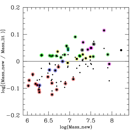
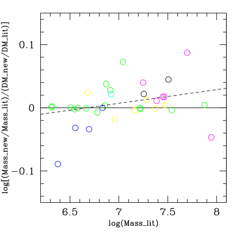
Figure 1: Left panel: The ratio between remodelled and previous literature estimates of dynamical masses of UCDs is plotted vs their remodelled mass. The original literature source is indicated by the colour coding of the circles around the data points. See Sect. 2.3 for details on the colour coding. For all the data points, we have recalculated the dynamical mass in this paper. Small dots (without a circle) indicate the ratio between the remodelled and literature dynamical mass-to-light ratio $M/L_{\rm dyn}$. Right panel: The ratio between remodelled and literature mass, cleaned of the effect of update in distance modulus, and without the CenA sample of Taylor et al. (2010), is plotted vs. the literature mass estimate.

2.3 Comparison of new and literature model masses

Based on the dynamical UCD masses derived above under the assumption that mass-follows-light we use the V-band apparent magnitudes from each literature source and their updated distance moduli to calculate the dynamical M/L ratios.

In Fig. 1 we plot the newly obtained dynamical masses vs. the ratio between this new estimate and the literature estimate. Note that all literature values were already based on a similar modelling as in this paper. We indicate as an aid for the eye as solid line the identity. The data points are colour coded according to the literature source of their original measurement. Blue circles refer to CenA UCDs originally from Rejkuba et al. (2007) with a first remodelling presented in Mieske et al. (2008). Yellow circles refer to Virgo UCDs originally from Haşegan et al. (2005) with a first remodelling presented in Mieske et al. (2008). Green circles refer to Fornax UCDs from Chilingarian et al. (2011), which itself is based on a remeasurement of spectroscopic data from Mieske et al. (2008) and a remodelling performed in Chilingarian et. al. (2011). The cyan circle refers to one Fornax UCD with designation F12 from Mieske et al. (2008). Red circles refer to UCDs in CenA from Taylor et al. (2010). Magenta circles refer to Virgo UCDs from Evstigneeva et al. (2007). Black circles indicate Fornax UCDs from Hilker et al. (2007). The object without a circle is Virgo UCD M59cO, from Chilingarian & Mamon (2008).

The median ratio between our newly modelled dynamical mass estimates and the literature values is 1.04 with an RMS scatter of 0.13. Similarly, the ratio between the new and literature $M/L_{\rm dyn}$ is 0.95 with an RMS scatter of 0.13. The opposite sense of difference in mass and mass-to-light ratio is mainly due to the updates in distance modulus for the Fornax and Virgo sources. They are between 3% and 8% larger than the distances adopted in the respective articles (see Table 1). Total masses increase linearly with distance, while M/L ratios decrease linearly since L scales quadratically with distance. The RMS scatter of 0.13 is not negligible when investigating individual sources in detail. Its value gives an indication of the systematic uncertainties in the determination of dynamical masses from integrated velocity dispersions, and should be considered for the total error budget of such measurements.

In the following we briefly discuss the one sample with a notable systematic offset between literature and remodelled mass, which is the CenA sample from Taylor et al. (2010).

2.3.1 CenA UCDs from Taylor et al. (2010).

The dynamical masses (and mass-to-light ratios) derived by Taylor et al. are on average 17% above our remodelled values, with an RMS of 6%. The fact that the average offset is larger than the scatter indicates a systematic relative bias in the mass calculation. Taylor et al. perform a modelling analogous to Hilker et al. (2007) and Mieske et al. (2008), to find the UCD model which represents best the measured velocity dispersion, given the spectroscopic aperture, seeing, and intrinsic light distribution of the source. However, unlike other studies, their finally quoted dynamical mass is not the total mass of the best fitting model. Instead, it is the dynamical mass derived from the modelled central velocity dispersion $\sigma_{0}$, via equation 3 of their paper: $M_{\rm dyn}=\frac{\beta\times\sigma_{0}^{2}\times r_{h}}{G}$. They adopt a value of $\beta=7.5$ for all their sources. They follow this approach of using $\sigma_{0}$ in order to contrast their measurement with literature data on other hot stellar systems which typically analyse scaling relations with $\sigma_{0}$.

Generally, $\beta$ is a scaling factor that varies strongly depending on the surface brightness profile. The typical ranges are between 5-10, see the literature review in Taylor et al. (2010). Thus, one expects an object-to-object scatter when comparing the results of Taylor et al. - which assume a fixed $\beta$ - to our remodelled masses which use the individual surface brightness profiles. The additional, systematic 17% average offset would be removed by adopting $\beta\sim 6.5$ instead of 7.5, which is still in the range of typical literature values for $\beta$. For example, Cappellari et al. (2006) find $\beta=5.0\pm 0.1$ for the central regions of early type galaxies and that $\beta$ varies by a factor of 2.5 amongst the objects in their sample. We thus conclude that the choice of a fixed $\beta$ is the most likely reason for the offset and scatter in the dynamical mass comparison between Taylor et al. (2010) and our remodelled data, noting that also in our analysis we make a simplifying assumption, namely an isotropic velocity distribution.

2.3.2 An overall trend?

In Fig. 1 left panel one notices an apparent trend in the sense that the ratio between new and literature mass increases with mass. To investigate the significance of this, we clean the sample in the following way, and replot it in the right panel. A) We remove the CenA sample from Taylor et al (2010), since this sample exhibits a systematic overall offset discussed above. B) We remove from the newly determined masses the effect of distance modulus update, reducing the mass estimates for the Fornax and Virgo sources between 3 and 8 %. C) We plot on the x-axis the literature mass estimate instead of the new mass estimate.

We then fit a linear relation to the data points. The resulting fit as indicated in the right panel of Fig. 1 yields a weak correlation with a slope of 0.021 $\pm$ 0.012 in log-log space between the mass ratio and the mass, which is significant at the 1.8$\sigma$ level. This corresponds to a 5% effect per dex in mass, or a range of $\pm 4\%$ between mean and extreme masses of the sample. In the context of our study this is negligible.

Table 3: Recalculated dynamical masses and further properties of UCDs in Centaurus A, Virgo, and Fornax. $\Psi$ is defined as $\Psi=(M/L)_{\rm dyn}/(M/L)_{\rm pop}$. The second-to-last column denotes the literature source of the original measurement of M_dyn,remod, and the origin of the [Fe/H] value. lit=1: Cen A UCDs from Mieske et al. (2008), based on original measurements presented in Rejkuba et al. (2007). lit=2: Virgo UCDs from Mieske et al. (2008), based on original measurements presented in Haşegan et al (2005). lit=3: Virgo UCDs from Evstigneeva et al. (2007). lit=3.2: The Virgo UCD M59cO from Chilingarian & Mamon (2008). lit=3.5: Fornax UCDs from Hilker et al. (2007). lit=7: CenA UCDs from Taylor et al. (2010), largely based on a re-reduction of data published in Rejkuba et al. (2007). lit=8: Fornax UCDs from Chilingarian et al. (2011), doing a remeasurement and re-modelling of spectroscopic data from Mieske et al. (2008). For objects marked with an asterisk ^∗, no unique King profile fit is available in the literature. Composite or single Sersic fits are adopted, see Sect. 2.1 for details. For VUCD7 and F19, the indicated King profile parameters r_c and $c$ are for the core component. For F19, the small error bar of 0.3 km/s for the measured velocity dispersion is due to the very high S/N spectrum obtained for this object, combined with the usage of the full spectral fitting technique (Chilingarian et al. 2011).

Name	Mdyn [10${}^{6}\rm\,M_{\odot}$]	[Fe/H]	MV	M/Ldyn	Mpop [10${}^{6}\rm\,M_{\odot}$]	$\Psi$	$\frac{M_{\rm dyn,thispaper}}{M_{\rm dyn,literature}}$	$\sigma$ [km/s]	rh [pc]	rc [pc]	$c$	lit	dist [Mpc]	BHfrac
M59cO∗	160 $\pm$ 34	-0.03	-13.26	9.6 $\pm$ 2.4	69	2.38 $\pm$ 0.59	1.10	48 $\pm$ 5	32	—	—	3.2	14.9	0.31${}^{+0.15}_{-0.12}$
VUCD7∗	86 $\pm$ 19	-0.66	-13.61	3.6 $\pm$ 0.93	68	1.27 $\pm$ 0.33	0.978	38.0 $\pm$ 4.1	105	—	—	3	16.5	0.027${}^{+0.03}_{-0.027}$
F19∗	80 $\pm$ 1.9	-0.19	-13.49	3.7 $\pm$ 0.49	77	1.03 $\pm$ 0.13	1.06	24.8 $\pm$ 0.3	90.6	3.7	1.7	8	20	0.003${}^{+0.014}_{-0.003}$
VUCD3	65 $\pm$ 4.6	-0.011	-12.75	6.1 $\pm$ 1.5	44	1.49 $\pm$ 0.37	1.30	42.1 $\pm$ 1.5	21.6	2.3	2.1	3	16.5	0.078${}^{+0.062}_{-0.057}$
UCD1	37 $\pm$ 2.3	-0.67	-12.19	5.8 $\pm$ 0.97	18	2.04 $\pm$ 0.34	1.16	32.0 $\pm$ 1.0	23.5	1.9	2.3	3.5	20	0.15${}^{+0.058}_{-0.04}$
F24	36 $\pm$ 2.5	-0.67	-12.37	4.8 $\pm$ 0.72	22	1.68 $\pm$ 0.25	1.04	29.1 $\pm$ 1.0	30.9	3.1	3.2	8	20	0.11${}^{+0.044}_{-0.038}$
VUCD5	33 $\pm$ 3.7	-0.36	-12.49	3.9 $\pm$ 0.77	28	1.17 $\pm$ 0.23	1.12	28.2 $\pm$ 1.6	19.2	7.1	1.4	3	16.5	0.042${}^{+0.055}_{-0.042}$
VUCD1	32 $\pm$ 3.1	-0.76	-12.43	3.9 $\pm$ 0.81	22	1.44 $\pm$ 0.3	1.12	34.1 $\pm$ 1.7	12.1	4.6	1.9	3	16.5	0.11${}^{+0.074}_{-0.065}$
S417	31 $\pm$ 3	-0.70	-11.84	6.6 $\pm$ 1.5	13	2.35 $\pm$ 0.53	1.04	30.5 $\pm$ 1.5	14.7	8.1	1.2	2	16.5	0.4${}^{+0.17}_{-0.15}$
VUCD4	27 $\pm$ 4.5	-1.10	-12.47	3.2 $\pm$ 0.95	21	1.31 $\pm$ 0.38	1.11	23.9 $\pm$ 2.0	23.6	6.3	1.7	3	16.5	0.071${}^{+0.083}_{-0.071}$
S999	24 $\pm$ 2.7	-1.40	-11.14	9.9 $\pm$ 1.9	5.5	4.4 $\pm$ 0.86	1.03	23.3 $\pm$ 1.3	20.7	13	1	2	16.5	1.1${}^{+0.25}_{-0.24}$
VUCD6	21 $\pm$ 3	-1.10	-12.27	3.0 $\pm$ 1.1	17	1.21 $\pm$ 0.45	1.18	25.2 $\pm$ 1.8	16.4	2.9	2.1	3	16.5	0.039${}^{+0.085}_{-0.039}$
S928	20 $\pm$ 1.8	-1.30	-11.64	5.3 $\pm$ 1.3	8.8	2.34 $\pm$ 0.59	1.06	20.0 $\pm$ 0.9	23.8	14	1.1	2	16.5	0.4${}^{+0.15}_{-0.14}$
UCD5∗	20 $\pm$ 4.5	-1.20	-12.10	3.4 $\pm$ 0.95	14	1.44 $\pm$ 0.41	1.10	22.9 $\pm$ 2.6	26.2	—	—	3.5	20	0.061${}^{+0.054}_{-0.048}$
F1	18 $\pm$ 0.95	-0.64	-12.29	2.5 $\pm$ 0.49	20	0.864 $\pm$ 0.17	1.05	22.2 $\pm$ 0.6	24.2	2.3	2.3	8	20	0${}^{+0.003}_{-0}$
F9	17 $\pm$ 1.9	-0.62	-11.43	5.4 $\pm$ 1.0	9.3	1.85 $\pm$ 0.36	1.05	28.4 $\pm$ 1.6	9.53	3.3	1.5	8	20	0.21${}^{+0.1}_{-0.085}$
S490	15 $\pm$ 1.9	0.18	-11.06	6.5 $\pm$ 1.4	11	1.4 $\pm$ 0.29	1.02	42.1 $\pm$ 2.7	3.74	0.7	1.8	2	16.5	0.088${}^{+0.068}_{-0.058}$
F8∗	14 $\pm$ 1.2	-0.35	-11.4	4.4 $\pm$ 1.1	10	1.32 $\pm$ 0.32	1.23	30.2 $\pm$ 1.3	6.7	—	—	8	20	0.087${}^{+0.085}_{-0.073}$
0330	12 $\pm$ 2.2	-0.36	-11.00	5.7 $\pm$ 1.3	7.1	1.72 $\pm$ 0.4	0.859	41.5 $\pm$ 3.7	3.26	0.86	1.7	7	3.77	0.17${}^{+0.099}_{-0.09}$
UCD12a	9.2 $\pm$ 1.5	-0.35	-11.60	2.5 $\pm$ 0.71	12	0.739 $\pm$ 0.21	1.1	23.9 $\pm$ 1.9	7.23	1.4	1.8	6	20	0${}^{+0.015}_{-0}$
F2∗	9.1 $\pm$ 1.7	-0.73	-11.45	2.8 $\pm$ 0.85	9	1.02 $\pm$ 0.31	1.12	19.9 $\pm$ 1.8	14.5	—	—	8	20	0.002${}^{+0.035}_{-0.002}$
S314	9 $\pm$ 0.72	-0.50	-10.97	4.3 $\pm$ 0.73	6.4	1.4 $\pm$ 0.24	0.987	35.2 $\pm$ 1.4	3.32	0.84	1.7	2	16.5	0.1${}^{+0.061}_{-0.057}$
F22	8.5 $\pm$ 0.87	-0.49	-11.22	3.2 $\pm$ 0.91	8.1	1.04 $\pm$ 0.3	1.14	29.1 $\pm$ 1.5	5.34	0.49	2.3	8	20	0.007${}^{+0.047}_{-0.007}$
0365	7.9 $\pm$ 1.6	-0.90	-11.05	3.5 $\pm$ 0.71	5.8	1.37 $\pm$ 0.39	0.827	23.7 $\pm$ 2.4	7.37	1.4	1.8	7	3.77	0.069${}^{+0.065}_{-0.053}$
F5	7.6 $\pm$ 0.6	-0.34	-11.83	1.7 $\pm$ 0.28	15	0.495 $\pm$ 0.083	1.06	25.4 $\pm$ 1.0	5.24	1.3	1.8	8	20	0
HGHH92-C1	6.8 $\pm$ 0.84	-1.2	-10.80	3.8 $\pm$ 0.96	4.2	1.62 $\pm$ 0.41	1.00	12.9 $\pm$ 0.8	23.3	7	1.6	1	3.77	0.11${}^{+0.078}_{-0.07}$
F17	6.2 $\pm$ 0.62	-0.55	-11.37	2.1 $\pm$ 0.44	9.1	0.687 $\pm$ 0.15	1.03	28.0 $\pm$ 1.4	3.46	0.94	1.7	8	20	0
0265	5.4 $\pm$ 1.5	-0.82	-10.59	3.7 $\pm$ 0.8	3.9	1.38 $\pm$ 0.49	0.953	20.8 $\pm$ 2.9	5.6	2.2	1.4	7	3.77	0.096${}^{+0.14}_{-0.096}$
H8005	5.2 $\pm$ 2.2	-1.30	-10.89	2.7 $\pm$ 1.5	4.5	1.16 $\pm$ 0.66	1.09	9.1 $\pm$ 1.9	29.5	14	1.3	2	16.5	0.043${}^{+0.19}_{-0.043}$
0320	4.9 $\pm$ 0.69	-0.90	-10.35	4.2 $\pm$ 0.6	3.1	1.62 $\pm$ 0.23	0.785	20.0 $\pm$ 1.4	6.84	1.2	1.9	7	3.77	0.13${}^{+0.051}_{-0.05}$
F11	4.9 $\pm$ 0.41	-0.61	-11.60	1.3 $\pm$ 0.27	11	0.447 $\pm$ 0.092	1.05	23.7 $\pm$ 1.0	3.77	1	1.7	8	20	0
VHH81-C5	4.6 $\pm$ 1.3	-1.40	-10.54	3.3 $\pm$ 0.73	3.1	1.48 $\pm$ 0.53	0.925	15.8 $\pm$ 2.2	8.8	5.9	0.89	1	3.77	0.12${}^{+0.16}_{-0.12}$
F7	4 $\pm$ 1	-1.20	-11.23	1.5 $\pm$ 0.55	6.2	0.635 $\pm$ 0.24	1.05	12.2 $\pm$ 1.6	11.9	7.2	1.2	8	20	0
0077	3.8 $\pm$ 0.69	-0.36	-10.34	3.3 $\pm$ 0.68	3.9	0.992 $\pm$ 0.2	0.753	16.7 $\pm$ 1.5	7.67	1.3	1.9	7	3.77	0${}^{+0.039}_{-0}$
0041	3.8 $\pm$ 0.78	-0.34	-10.13	4.0 $\pm$ 0.87	3.2	1.18 $\pm$ 0.26	0.83	17.6 $\pm$ 1.8	6.76	1.2	1.9	7	3.77	0.035${}^{+0.056}_{-0.035}$
F51	3.7 $\pm$ 0.56	-0.23	-10.66	2.3 $\pm$ 0.72	5.6	0.661 $\pm$ 0.2	1.05	20.9 $\pm$ 1.6	4.4	0.51	2.5	8	20	0
F6	3.4 $\pm$ 1	-1.30	-11.17	1.3 $\pm$ 0.51	5.7	0.591 $\pm$ 0.22	1.05	14.0 $\pm$ 2.1	7.64	2.4	1.6	8	20	0
HGHH92-C6	3.3 $\pm$ 0.48	-0.91	-11.01	1.5 $\pm$ 0.37	5.6	0.596 $\pm$ 0.14	0.929	20.7 $\pm$ 1.5	4.3	0.57	2.4	1	3.77	0
0326	3.1 $\pm$ 0.57	-1.0	-10.07	3.4 $\pm$ 0.69	2.3	1.35 $\pm$ 0.27	0.876	19.4 $\pm$ 1.8	3.73	1.1	1.6	7	3.77	0.082${}^{+0.067}_{-0.062}$
F34	2.2 $\pm$ 0.43	-0.77	-10.83	1.2 $\pm$ 0.37	5	0.441 $\pm$ 0.13	1.06	15.3 $\pm$ 1.5	4.19	1.4	1.5	8	20	0
F53	2.1 $\pm$ 0.53	-0.80	-10.65	1.4 $\pm$ 0.49	4.2	0.513 $\pm$ 0.18	1.05	14.5 $\pm$ 1.8	4.71	0.95	2	8	20	0
VHH81-C3	1.9 $\pm$ 0.27	-0.22	-10.51	1.4 $\pm$ 0.37	4.9	0.397 $\pm$ 0.1	0.815	16.1 $\pm$ 1.1	4.2	0.47	2.6	1	3.77	0
0372	1.9 $\pm$ 0.42	-1.20	-9.84	2.6 $\pm$ 0.73	1.7	1.12 $\pm$ 0.31	0.769	16.5 $\pm$ 1.8	3.54	0.68	2	7	3.77	0.023${}^{+0.068}_{-0.023}$
0227	1.9 $\pm$ 0.33	-1.30	-9.56	3.3 $\pm$ 0.6	1.3	1.46 $\pm$ 0.26	0.784	13.6 $\pm$ 1.2	5.6	1.2	1.7	7	3.77	0.099${}^{+0.075}_{-0.057}$
0218	1.7 $\pm$ 0.43	-0.49	-9.69	2.7 $\pm$ 0.88	2	0.863 $\pm$ 0.28	0.817	12.7 $\pm$ 1.6	5.23	1.2	1.9	7	3.77	0${}^{+0.032}_{-0}$
0040	1.6 $\pm$ 0.3	-0.41	-9.69	2.4 $\pm$ 0.54	2.1	0.76 $\pm$ 0.17	0.825	13.7 $\pm$ 1.3	4.43	0.77	1.9	7	3.77	0
0378	1.3 $\pm$ 0.25	-0.51	-9.79	1.9 $\pm$ 0.56	2.2	0.623 $\pm$ 0.18	0.895	14.2 $\pm$ 1.3	3.26	0.58	1.9	7	3.77	0
0150	1.1 $\pm$ 0.17	-0.54	-10.05	1.2 $\pm$ 0.2	2.7	0.409 $\pm$ 0.067	0.85	15.9 $\pm$ 1.2	1.92	0.4	2	7	3.77	0
0232	1.1 $\pm$ 0.31	-0.77	-9.45	2 $\pm$ 0.78	1.4	0.753 $\pm$ 0.28	0.812	14.1 $\pm$ 2.1	2.6	0.5	2	7	3.77	0${}^{+0.011}_{-0}$

Table 3: continued.

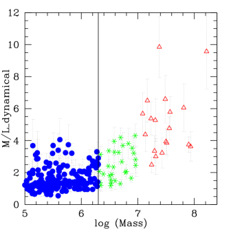
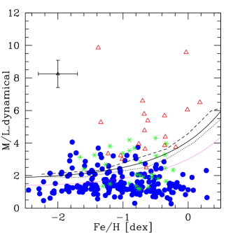
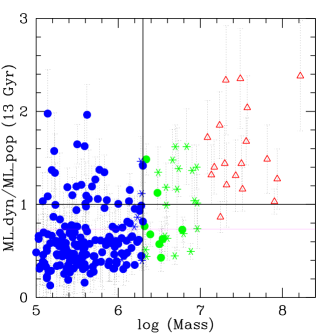
Figure 2: Left panel: Dynamical mass-to-light ratios of compact stellar systems plotted vs. their dynamical mass. Data taken from the literature as indicated in the text. Sources are colour coded according to mass. GCs ($M<2*10^{6}\rm\,M_{\odot}$) are blue, low-mass UCDs ($2*10^{6}\rm\,M_{\odot}<M<10^{7}\rm\,M_{\odot}$) are green, high-mass UCDs ($M>10^{7}\rm\,M_{\odot}$) are red. GC data points are dominated by Local Group measurements, whereas UCD data points are mainly extragalactic (Fornax/Virgo/CenA). Middle panel: Dynamical mass-to-light ratios of compact stellar systems plotted vs. their metallicities. Sample and symbols as in the left panel. The dotted lines correspond to predicted stellar M/L ratios for a 13 Gyr stellar population of solar $\alpha$ abundance; top line is from Maraston et al. (2005), bottom line is from Bruzual & Charlot (2003). The solid curve in between is an exponential fit to the mean of the two dotted lines. It represents the maximum stellar M/L for a canonical IMF (Kroupa/Chabrier). Sources with dynamical M/L ratios above that solid line need some extra dark mass, and/or IMF variation. The (magenta) thin solid line below the thick solid line corresponds to the stellar M/L ratio for a younger, 9 Gyr stellar population of solar $\alpha$ abundance. Right panel: The dimensionless quantity $\Psi=(M/L)_{\rm dyn}/(M/L)_{\rm pop}$ is plotted vs. dynamical mass for the same sources as in previous plots, using equation 4 for $(M/L)_{\rm pop}$, see also middle panel. The black horizontal line indicates $\Psi=1$ for 13 Gyr assumed age (see also black solid line in middle panel), the (magenta) thin solid line indicates $\Psi=1$ for 9 Gyr assumed age (magenta solid line in middle panel). We mark UCDs ($M>2*10^{6}\rm\,M_{\odot}$) from the Local Group with (green) filled circles, and massive extragalactic GCs ($M<2*10^{6}\rm\,M_{\odot}$) with (blue) asterisks.

2.4 Distribution of dynamical M/L vs. mass

In Table LABEL:tableall we list the updated dynamical masses and dynamical M/L ratios for the compact stellar systems considered, along with the mass difference to the original publication. We also report their absolute magnitudes, stellar population masses, literature measured velocity dispersion, effective radius, metallicity, adopted structural profile parameters and distance used in the modelling.

In the left panel of Fig. 2 we plot the updated measurements of mass versus dynamical M/L ratio of the above sources. For comparison we also include the most recent data on compact stellar systems for the Milky Way (Mc Laughlin & van der Marel 2005) and M31 (Strader et al. 2009). We reproduce the previously known trend (Mieske et al. 2008) that the dynamical M/L of compact stellar systems above $2\times 10^{6}\rm\,M_{\odot}$ - the regime of UCDs - increase with mass. We colour code the sources according to mass: GCs ($M<2*10^{6}\rm\,M_{\odot}$) are blue, low-mass UCDs ($2\times 10^{6}\rm\,M_{\odot}<M<10^{7}\rm\,M_{\odot}$) are green, high-mass UCDs ($M>10^{7}\rm\,M_{\odot}$) are red.

In the middle panel of Fig. 2 we plot the dynamical M/L ratio vs. metallicity [Fe/H]. The lines correspond to predicted stellar M/L ratios for a 13 Gyr stellar population of solar $\alpha$ abundance; dashed line is from Maraston et al. (2005), dotted line is from Bruzual & Charlot (2003). The solid line is the mean of exponential fits to the two models, given by the quantity $(M/L)_{\rm pop}$ introduced in equation 4, thus being the maximum stellar M/L for a canonical (e.g. Kroupa 2002) IMF.

It is evident that many GCs are located significantly below that ridge line, in particular the more metal-rich GCs. This was reported already by Strader et al. (2009, 2011). This is interesting in its own right and may indicate an IMF variation. In the present paper, we focus however on the most massive compact stellar systems, the UCDs. Almost all of the massive UCDs have dynamical M/L above the ridge line, consistent with dark mass on top of a canonical IMF.

In the right panel of Fig. 2 we plot for each source the dimensionless quantity

$$\Psi=(M/L)_{\rm dyn}/(M/L)_{\rm pop}$$ (5)

defined as the ratio between dynamical and stellar population M/L ratio. $\Psi$ above unity indicates the presence of non-luminous mass on top of a canonical stellar population (assuming virial equilibrium). For calculating $\Psi$, the dynamical M/L ratio is taken from the top left panel, and the stellar population M/L ratio is taken from equation 4.

The plotted uncertainty of $\Psi$ is a Gaussian propagation of two main error contributions. 1. the uncertainty of the dynamical M/L, which itself encompasses the error bar of the velocity dispersion, distance estimate, luminosity, surface brightness profile. 2. An assumed global 0.3 dex uncertainty in the sources’ [Fe/H], translated to an uncertainty factor of $(M/L)_{\rm pop}$ (Mieske et al. 2008).

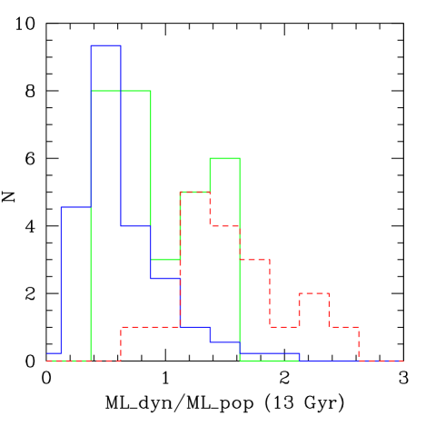
Figure 3: Histogram of $\Psi=(M/L)_{\rm dyn}/(M/L)_{\rm pop}$ for the samples of Fig. 2. The (dashed) red histogram denotes high-mass UCDs with $M>10^{7}\rm\,M_{\odot}$. The green (solid) histogram denotes low-mass UCDs $2\times 10^{6}\rm\,M_{\odot}<M<10^{7}\rm\,M_{\odot}$. The blue (solid) hostogram denotes globular clusters ($M<2\times 10^{6}\rm\,M_{\odot}$). The histogram for GCs is scaled down by a factor of 9 to fit the plot. The low $\Psi$ peak of the green histogram is close to the peak of the blue (GC) sample. The shift of $\sim$20% between those two peaks is expected from dynamical evolution (e.g. Baumgardt & Makino 2003, Kruijssen & Mieske 2009).

2.4.1 A bimodal M/L distribution for low-mass UCDs

In Fig. 3 we show the histogram of $\Psi$ for GCs, low-mass UCDs, and high-mass UCDs. The 19 high-mass UCDs ($M>10^{7}\rm\,M_{\odot}$) have a median $\Psi$ of 1.45, with a mean of 1.73 $\pm$ 0.19. The 30 low-mass UCDs ($M<10^{7}\rm\,M_{\odot}$) have an average $\Psi$ of 0.93 $\pm 0.07$, consistent with, on average, a ’normal’ stellar population. From the histogram morphology there is a hint for a bimodal distribution in $\Psi$ in the low-mass sample with a dip around $\Psi\sim 1$. We use the KMM tool (e.g. Ashman et al. 1994) to test the significance of this possible bimodality in the $\Psi$ distribution. We run KMM in homoscedastic mode, which means that a single (Gaussian) width is assumed for each of the two potential subpopulations. The KMM test yields the following results: the low-mass sample is inconsistent with a single Gaussian distribution in $\Psi$ at the 99.2% confidence level. KMM finds two distinct Gaussian peaks at $\Psi=0.63$ and $\Psi=1.33$ of width $\sigma=0.17$, containing 14 and 16 UCDs, respectively. In contrast, the high-mass sample cannot be fitted with a bimodal Gaussian. All 19 sources in this sample are assigned to one single Gaussian by KMM, peaked at $\Psi=1.73$ with a width $\sigma=0.77$.

The bimodal $\Psi$ distribution for low-mass UCDs and the offset unimodal $\Psi$ distribution for high-mass UCDs are an intriguing finding. It is consistent with the hypothesis that in the low-mass UCD regime there is indeed an overlap between massive globular clusters (with normal M/L ratios) and UCDs as stripped nuclei (with elevated M/L ratios), and that the latter population dominates the high-mass UCDs.

2.4.2 On the assumption of single stellar populations

There is one potential concern when comparing the observed dynamical M/L of UCDs to single stellar population (SSP) predictions of stellar M/L: if UCDs are remnant nuclei of galaxies, or resemble massive GCs, it is likely that they contain multiple stellar populations. Is it therefore appropriate to compare the dynamical M/L to the predictions of SSP models?

If a young population is present on top of an underlying old population, the integrated light in the optical, and therefore the spectroscopic population parameters available in the literature, will be dominated by the young population, even if this population contributes only a small fraction of the stellar mass. Thus, based on spectroscopic population parameters, the mass-weighted age of composite population UCDs would be underestimated. Assuming a reasonable enrichment history with younger populations being at least as enriched as older populations, their mass-weighted metallicities would be overestimated by the spectroscopic value. Moreover, also purely old, metal-poor ([Fe/H]$\lesssim-1.2$ dex) stellar populations can mimic a young population in integrated-light spectroscopy, if they contain blue horizontal branch stars (Ocvirk 2010). Since younger and/or more metal-poor populations have a lower stellar M/L, underestimating the metallicity or age would lead to an underestimation of the true mass-weighted stellar population M/L_pop.

However, if one uses only spectroscopic metallicity measurements (that will tend to be over- but not underestimated in the presence of younger stellar populations), and adopts an old age for safety, even if spectroscopic indices may indicate differently, one will not underestimate, but potentially overestimate, the M/L_pop of UCDs.

Hence, the apparent surplus of dynamical M/L for massive UCDs cannot be explained as the result of the presence of multiple stellar populations. In fact, in the presence of multiple populations, the discrepancy between dynamical and stellar population M/L may be even higher than our estimates.

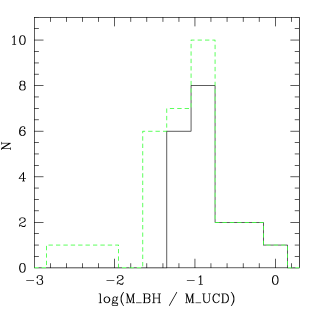
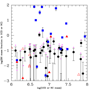
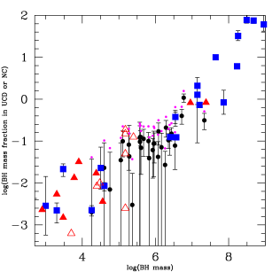
Figure 4: Left panel: Histogram of the black hole mass fraction as estimated for those UCDs with $\Psi=(M/L)_{\rm dyn}/(M/L)_{\rm pop}>1$, see Sect. 3. The solid histogram corresponds to BH mass estimates whose lower 1 $\sigma$ error bound is above 0. The dashed (green) histogram includes also those UCDs for which the lower 1 $\sigma$ error bound is consistent with 0. Middle panel: Black hole mass fraction in compact stellar systems plotted vs. the stellar mass of the compact stellar systems. Filled black circles are the UCDs from the left panel. The UCD mass used on the x-axis is the stellar population mass M_pop for an age of 13 Gyr. The small filled (magenta) circles indicate the modelled BH mass assuming a stellar population age of 9 Gyr. Filled blue squares are BH mass measurements in nuclear clusters from Graham et al. (2009) which have a lower BH mass limit larger than 0. Filled (red) triangles are those sources from Graham et al. for which the BH mass is an upper limit. Open (red) triangles are upper limits for BHs in lower mass nuclear clusters from Neumayer & Walcher (2012). Right panel: Black hole mass fraction in compact stellar systems plotted vs. the black hole mass, for the same objects as in the middle panel.

Figure 5: Left panel: For those galaxies with a BH and a NC in the sample of Graham et al. (2009), we plot the ratio between BH and NC mass vs. the total bulge mass of the host galaxy. A least square linear fit through the data points is indicated as dotted line. The horizontal dotted and dashed lines indicate the median and rms scatter of BH mass fraction in UCDs, see Fig. 7. The typical host galaxy bulge masses for those nuclei that have a BH mass fraction comparable to UCDs is 10^9±1 solar masses. Right panel: Analogous to the left plot, we give on the x-axis the ratio of NC over host galaxy bulge mass. The typical NC/bulge mass fraction is $\sim$1% in the range of BH/NC mass fraction of UCDs. We do not plot a linear fit to the literature data due to their larger scatter compared to the left panel.

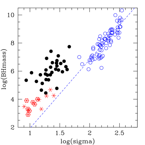
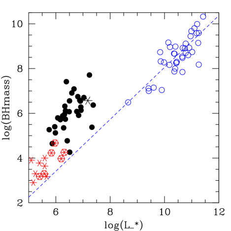
Figure 6: Left Panel: M_BH-$\sigma$ relation for UCDs (black filled circles), compared to Galactic GCs (red asterisks, Lützgendorf et al. 2013; sources with hexagons have only upper limits to their BH mass) and galaxies (blue circles; McConnell et al. 2013). The blue dashed line is a linear fit in log-log space to the galaxy sample. It has a slope of 4.9. The BH mass of UCDs is on average offset by about 2 dex from this relation. Right panel: M_BH-Luminosity relation for the same sources as in the left panel. Some objects from the galaxy sample of McConnell et al. are not included here since they lack information on host galaxy luminosity. The blue dashed line is a linear fit in log-log space to the galaxy sample with a slope of 1.16, indicating near direct proportionality between BH mass and host luminosity. The luminosity of UCDs is on average offset by 2 dex with respect to this reference. For illustration purposes we also show as large asterisk the central black hole mass of the Milky Way vs. the luminosity of the Milky Way’s nuclear cluster (Graham & Spitler 2009).

3 BH mass estimates in UCDs

In the following we provide an estimate of the mass of a hypothetical central BH for those UCDs whose dynamical mass exceeds the stellar population mass, that is for those UCDs with $\Psi=(M/L)_{\rm dyn}/(M/L)_{\rm pop}>1$ in Fig. 2 right panel. In doing so, we assume that the gravitational potential of the BH is responsible for the elevated overall velocity dispersion which gives rise to the nominally high dynamical M/L:

1. We continue after the first step outlined in Sect. 2.2 for determining the observed velocity dispersion $\sigma_{\rm\rm obs,pop}$ for the stellar population mass of the UCDs.

2. In order to determine BH masses for the UCDs, we add point-mass potentials $-GM_{\rm BH}/r$ with varying mass fractions $M_{\rm BH}/M_{\rm UCD}$ to the potentials based on the stellar distribution calculated in step 2 of sec. 2.2 of each UCD. We then determine new distribution functions f(E) and velocity distributions for the stars in the combined potentials.

3. We then calculate the predicted velocity dispersions seen by the observers as outlined in steps 3 to 5 of sec. 2.2 and determine the BH mass fractions which lead to an agreement of the observed velocity dispersion with the predicted ones.

4. To estimate the uncertainty of the BH mass, we assign the full measurement uncertainty of the dynamical mass-to-light ratio to the observed velocity dispersion, which can be denoted as $\Delta\sigma_{\rm obs,total}$, and redetermine the BH mass for $\sigma_{\rm\rm obs,new}=\sigma_{\rm\rm obs}\pm\Delta\sigma_{\rm obs,total}$. To obtain $\Delta\sigma_{\rm obs,total}$, we first separate the literature uncertainty $\Delta\sigma_{\rm obs}$ of the observed velocity dispersion $\sigma_{\rm obs}$ from the overall error of $\Psi$. For this we assume Gaussian propagation, and that the relative contribution of the $\sigma$ error to the M/L uncertainty is $2\frac{\Delta\sigma}{\sigma}$. The resulting residual error is the uncertainty of the stellar population mass, and we denote it $\Delta_{\rm Mpop}$. For a constant BH mass fraction, an uncertainty $\Delta_{\rm Mpop}$ in the stellar population mass will lead to a change of the predicted velocity dispersion by $\Delta\sigma_{\rm obs,fromM/L}=\sigma(\sqrt{1+\frac{\Delta_{\rm Mpop}}{M_{pop}}}-1)$. Since this uncertainty is statistically independent of the measurement uncertainty $\Delta\sigma_{\rm obs}$, it will lead to a combined uncertainty $\Delta\sigma_{\rm obs,total}=\sqrt{\Delta\sigma_{\rm obs,fromM/L}^{2}+\Delta\sigma_{\rm obs}^{2}}$.

5. Not all of the studied UCDs may necessarily be consistent with an assumed age of 13 Gyrs, which is a conservative assumption in the context of this study - $\Psi$ is lower for older ages. We therefore repeat the above steps also for a stellar population mass corresponding to a younger age of 9 Gyr. According to the models of Bruzual & Charlot (2003) and Maraston (2005) the expected stellar population mass is a factor of 1.36 below the stellar population mass for 13 Gyr, see Fig. 2. That is, the BH mass obtained for an assumed age of 9 Gyr will always be above the BH mass for 13 Gyr, since $\Psi_{\rm 9Gyr}=1.36\times\Psi_{\rm 13Gyr}$.

The resulting histogram of inferred BH mass fractions is shown in the left panel of Fig. 4. The median BH mass fraction for UCDs with significant BH masses (lower error bar above 0) is 11%. In the left and middle panels of that figure we compare these fractions to literature data of BH masses in galaxy nuclear clusters (NCs; Graham et. al. 2009, Neumayer & Walcher 2012). We note that the BH masses from Neumayer & Walcher are all upper limits. The middle panel shows the BH mass fraction vs. UCD and NC mass. The right panel shows the BH mass fraction vs. the BH mass. In those two panels we also show as small (magenta) dots the BH mass estimates for UCDs assuming an age of 9 Gyr for the stellar population. The median BH mass for this case is 14%.

4 Discussion

4.1 BH mass fractions in UCDs and NCs, and the link to host galaxies

One commonly discussed formation scenario of UCDs is the tidal stripping of a more massive host galaxy, which leaves only the most compact central object (its nucleus) intact (e.g.Bekki et al. 2003, Pfeffer & Baumgardt 2013). Graham et al. (2009) provide a compilation of literature measurements for galaxies that have both a nuclear cluster and a central black hole. In the left panel of Fig. 5 we plot the ratio of BH mass over NC mass vs. the bulge mass of the respective host galaxies. We indicate as dotted line a linear least square fit to the data. As horizontal dashed lines we indicate the typical BH mass fraction that we estimate for UCDs in the previous section.

If UCDs are ’naked nuclei’ harbouring central BHs as fossil relics of their progenitor galaxies, the BH masses can be used to constrain their origin. With Fig. 5 one can pose the question: what is the host galaxy mass for NCs that contain a BH of about 10% of the NC’s mass? From the left panel of Fig. 5 one thus estimates, in the framework of the stripping hypothesis, a typical UCD host mass of 10${}^{9}\rm\,M_{\odot}$, with a range between 10${}^{8}\rm\,M_{\odot}$ to 10${}^{10}\rm\,M_{\odot}$ solar masses. The right panel of the same figure shows that this corresponds to a typical mass fraction of $\sim$1% between NC and host. Numerical simulations of galaxy tidal stripping predict a mass fraction of a few percent between tidally stripped naked nucleus and the original host (e.g. Bekki et al. 2003, Pfeffer & Baumgardt 2013), which also leads to typical progenitor masses of $\sim 10^{9}\rm\,M_{\odot}$.

Thus, the BH mass fractions of around 10% estimated for UCDs based on their elevated M/L ratios agree well with BH mass fractions of ’naked nuclei’ expected in the tidal stripping scenario. At the same time, such BH mass fractions rule out the hypothesis that most UCDs are hyper-compact stellar systems bound to recoiling super-massive black holes that were ejected from the centres of massive galaxies (Merritt et al. 2009). For such hypothetical objects one would expect BH masses comparable to or larger than the stellar mass.

4.2 Fraction of UCDs with significant BH masses

From our full sample of 49 UCDs, we find 18 UCDs are consistent with a formal BH mass of zero and 31 sources require a formal BH mass above zero. Of those 31 UCDs, 19 also have their lower BH mass limits above zero. That is, 19 UCDs ($\sim$40% of all) formally require at the 1$\sigma$ level some additional dark mass to account for their elevated dynamical M/L ratio. We re-iterate that our M/L threshold for requiring dark mass assumes a 13 Gyr age for a canonical stellar population. This is a conservative limit which may assign too low dark mass fractions to some UCDs, if their light were dominated by a stellar population substantially younger than 13 Gyr (Sect. 2.4.2 of this paper) or if they have been subject to significant dynamical evolution (Kruijssen & Mieske 2009).

Under the assumption that the IMF in UCDs is canonical (e.g. following a Kroupa 2002 parametrisation), one can thus speculate that about half of the UCD population may contain a central BH with a mass sufficient to notably elevate the measured velocity dispersion. In this context, the term ’notably’ refers to the observationally derived error bars of the ratio between final dynamical M/L measurement and stellar population M/L, which includes a general 0.3 dex error bar in [Fe/H]. The top left panel of Fig. 7 plots the estimated BH fraction in UCDs vs. the 1 $\sigma$ uncertainty of that estimate (lower limit). No BH mass estimate is more accurate than $\sim$20% relative error. Furthermore, only eight of the UCDs in our sample have relative errors $<50\%$, i.e. a $>2\sigma$ significant BH mass estimate (seven of those are high-mass UCDs with $M>10^{7}\rm\,M_{\odot}$). This 2$\sigma$ significance limit coincides with a BH mass fraction of about 10%.

4.2.1 BH occupation fraction in high-mass vs. low-mass UCDs

It has been shown in Sect. 2.4.1 that the distribution in $\Psi$ for high-mass UCDs is unimodal with a mean $\Psi\sim 1.7$, while for low-mass UCDs the distribution appears bimodal with peaks at $\sim$0.6 and $\sim$1.3. This is naturally also reflected in the BH mass distribution of the two sub-samples. Of the 19 UCDs that formally require a BH at the 1$\sigma$ level, 13 are high-mass UCDs (2/3 of all high-mass UCDs) and 6 are low-mass UCDs (1/5 of low-mass UCDs). In contrast, within the 18 UCDs that have formal BH masses of 0, there is only one single high-mass UCD. See Table LABEL:tableall.

Under the assumption that all high-mass UCDs are naked nuclei our data would thus suggest that 60-100% of the UCD progenitor galaxies in our sample possessed a SMBH.

Among the 30 low-mass UCDs, 13 have formal BH masses above zero and 17 UCDs have formal BH masses of zero. This approximate equipartition between UCDs with and without BH is a consequence of the above mentioned bimodal distribution in $\Psi$ for low-mass UCDs. As mentioned in Sect. 2.4.1, this could be explained if the transition mass regime $2\times 10^{6}<M<10^{7}\rm\,M_{\odot}$ is populated both by the high-mass extension of the canonical globular cluster population, and the low-mass tail of tidally stripped nuclear clusters. In the next subsection we elaborate more on this possibility from a statistical point of view.

4.3 Star clusters vs. tidally stripped nuclei

In Mieske et al. (2012) it was shown that the overall number counts of UCDs are consistent with being a simple extrapolation of the globular cluster luminosity function towards brighter luminosities. An upper limit of $\sim$50% of contamination from an additional formation channel was derived in that work.

Based on these numbers it is argued in Mieske et al. (2012) that it is not necessary to invoke an additional formation channel for UCDs. We stress here that this is not in contrast to the above formulated hypothesis that the most massive UCDs originate (mainly) from tidally stripped dwarf galaxies, because those massive UCDs are only a small fraction of the full UCD regime, see next paragraph. Also, the contamination of up to 50% of tidally stripped nuclei in the low-mass UCD regime $M<10^{7}\rm\,M_{\odot}$ as suggested in Sect. 2.4 and  4.2.1 is still within the range ’allowed’ by the upper contamination limit derived in Mieske et al. (2012).

The respective mass threshold of $M\sim 10^{7}\rm\,M_{\odot}$ corresponds to a luminosity of $M_{V}\simeq-11.5$ mag, when assuming M/L$\sim$3 (Fig. 2). This is about 1.3 mag brighter than the luminosity limit of $M_{V}=-10.2$ mag adopted for UCDs in Mieske et al. (2012) - calculated for a mass of $M=2\times 10^{6}\rm\,M_{\odot}$ and a M/L=2 (Fig. 2). A typical globular cluster luminosity function peaks around $M_{V}=-7.4$ mag and has a width of $\sim$1.3 mag (Mieske et al. 2012 and references therein). Based on the normal distribution, the number of objects with $M_{V}<-11.5$ mag (=3.15$\sigma$ away from the Gaussian peak) is only 0.001 of the whole population, and only 6-7% of the entire UCD population with $M_{V}<-10.2$ mag (=2.15$\sigma$ away from the peak). The fact that in Fig. 2 the relative fraction of massive UCDs with $M>10^{7}\rm\,M_{\odot}$ is much larger ($\sim$40%) is due to the higher observational completeness in the bright luminosity regime.

Fig. 5 of Mieske et al. (2012) compares for the Fornax cluster the cumulative distribution of galaxies in the expected UCD progenitor mass range (Bekki et al. 2003) to the cumulative distribution of present-day UCDs. The present-day number of potential progenitor galaxies is more than an order of magnitude lower than the total number of UCDs when considering all UCDs with $M_{V}<-10.2$. The numbers of UCDs and potential progenitors become comparable, and hence more consistent with theoretical predictions (Henriques et al. 2008, 2010), for UCD luminosities $M_{V}\lesssim-11.5$ mag. This coincides with the limit above which there appears systematic evidence for additional dark mass in UCDs, and is again consistent with the notion that tidally stripped galaxies dominate over the star cluster channel only in the high mass UCD regime.

4.4 The location of UCDs in the M_BH-$L$ and M_BH-$\sigma$ plane

Further insight into the nature of UCDs can be gained by placing them on the well known M_BH-L and M_BH-$\sigma$ relation (e.g. Ferrarese & Merritt 2000), using the putative BH masses estimated above. In Fig. 6 we show in the left panel the global velocity dispersions of the UCDs in our sample vs. these BH masses, plotted in log-log-space. The right panel plots the total luminosity vs. BH mass. For comparison we indicate central black hole mass estimates in Galactic globular clusters from Lützgendorf et al. (2013) with red asterisks, and the galaxy sample from McConnell et al. (2013) as blue open circles. We also show as dashed line a linear fit in log-log space to the galaxy sample. The slope is 4.9 for the M_BH-$\sigma$ relation, and 1.2 for the M_BH-$L$ relation of the galaxy sample.

In the M_BH-$L$ plane UCDs are offset towards lower luminosities by about a factor of 100 compared to the relation defined by galaxies. In the M_BH-$\sigma$ plane UCDs show an analogous offset of about 2 dex in BH mass with respect to the relation defined by galaxies. This suggests that in the framework of the tidal stripping scenario, today’s UCDs would have $\sim$1% of the luminosity of their potential progenitor galaxy. For nuclear clusters in present-day galaxies, the right panel of Fig. 5 shows that such a ratio of $\sim$1% is typical for nuclei that have BH mass fractions of $\sim$10%, as estimated for UCDs.

This lends further plausibility to the hypothesis that some UCDs are created by tidal stripping, having kept the massive central black hole as a relict tracer of their much more massive progenitor galaxies (Bekki et al. 2003, Pfeffer & Baumgardt 2013). It is interesting to note in the right panel of Fig. 6 that the MW’s nuclear cluster, if considered as single object without its host galaxy, is consistent with the postulated location of UCDs: the MW BH has about 1/10th of the nuclear cluster’s mass (Graham & Spitler 2009 and references therein).

A basic sanity check of this scenario is to combine the factor 100 offset to the $M_{\rm BH}-$Luminosity relation of galaxies with the 10-15% BH mass fractions in UCDs. The implied BH mass fraction in UCD progenitor galaxies would then be of order $\sim$0.1-0.2%, indeed close to the 0.2% BH mass fractions found generally in galaxies (e.g. Ferrarese et al. 2006). This is, however, not an independent argument per se, since the location of the $M_{\rm BH}-$Luminosity relation for galaxies is what defines the overall $\sim$0.2% BH mass fraction.

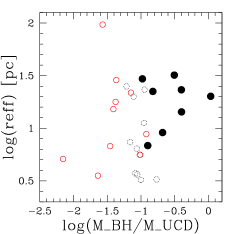
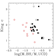
Figure 7: Top left panel: BH mass fraction of UCDs plotted vs. its relative error. Sources with relative error of one are those where the lower error bar of the BH mass is consistent with 0. BH mass estimates more significant than $\sim$2$\sigma$ require $\gtrsim$10% BH mass. Top right panel: BH mass fraction plotted vs. the effective radius in arcseconds. Red open circles are those objects where the lower error bounds of the dynamical mass measurements are consistent with zero BH mass. Dotted black circles denote those UCDs whose BH mass estimate is different from zero between 1 and 2$\sigma$ significance. Filled black circles indicate those UCDs with black hole masses more than 2$\sigma$ significant. These are those with relative error $<0.5$ in the top left panel. Bottom left panel: BH mass fraction in UCDs is plotted vs. the concentration parameter $c$ of their surface brightness distribution, when parametrised as a King profile. The filled dots indicate the BH mass fraction assuming that all UCDs have the same King parameter $c$ of 1.75, taking into account the correlation between $c$ and BH mass as shown in the right panel. Bottom right panel: The y-axis shows the concentration parameter $c$ as in the left panel. The x-axis shows the ratio between the BH mass fraction and the additional dynamical mass derived under the assumption that mass follows light, ($\Psi-1$). The fact that this ratio is generally below 1 is because the putative BH is located in the center of the UCD, as opposed to a uniformally distributed additional mass component. The overall trend is due to the fact that for more centrally concentrated objects, the effect of the BH on the integrated velocity dispersion increases. On average, a central BH of a given mass has the same effect on the global velocity dispersion as 4-5 times that mass distributed uniformally.

4.5 Dependence of UCD BH mass on structural parameters

It is commonly argued that the presence of a central black hole in the center of a galaxy can affect the stellar distribution, up to the point where a previously existing nucleus is entirely evaporated (e.g. Côté et al. 2006, Bekki & Graham 2010, Antonini et al. 2013). It is thus interesting to test whether structural parameters of the UCDs in our sample correlate with the hypothetical BH mass fraction. In Fig. 7 we show two plots that relate the hypothetical BH mass in UCDs to the UCDs’ structural parameters.

The top right panel plots the relative BH mass against the effective radius. No dependence between both entities is found.

The bottom left panel of Fig. 7 depicts the relative BH mass as a function of central concentration of the light profile (parametrised by the King concentration c). Considering those sources whose hypothetical BH mass is significant beyond the 1$\sigma$ individual error bar, a trend may be seen. A least squares fit to the data points reveals a correlation with a slope different from zero at the 2.8$\sigma$ level significance level. The Spearman correlation coefficient is $\rho=-0.543$, with a probability of 3% that there is no correlation. Also a Pearson and a Kendall test yield similar probabilities of 2-3%. The formal significance of this trend is thus between 2-3$\sigma$.

The bottom right panel depicts the King concentration parameter against the ratio between BH mass fraction and dynamical M/L surplus, $\Psi-1$. This ratio illustrates by how much more a central BH of a given mass influences the global velocity dispersion compared to a uniformly distributed dark mass component. The effect of a central BH on the global velocity dispersion is typically a factor of 4-5 higher than the effect of the same amount of mass in uniform distribution. Aside this general offset, there is also a clear trend in the sense that a central BH alters the global velocity dispersion stronger for sources with higher King concentration parameter. This is qualitatively expected, since a higher central concentration implies a larger relative number of stars within the sphere of influence of the BH.

The trend shown in the bottom right panel may also, at least partially, explain the trend between King concentration parameter and BH fraction seen in the bottom left panel. If one were to assume, conservatively, that all UCDs have the same intrinsic concentration $\sim$ 1.75, and that the distribution of concentrations measured in the literature are merely due to measurement uncertainties, then the resulting BH mass fractions would need to be renormalised to that same average concentration, based on the relation seen in the bottom right panel. The result of such an exercise is shown by the small filled circles in the bottom left plot: the BH mass fraction are ’corrected’ to an assumed true King concentration of 1.75. For this case, the correlation between King concentration and BH mass fraction is removed (the formal significance drops to the 1.4% level). We note that typically quoted uncertainties of King concentration (which itself is a logarithm) are 0.1 to 0.2 in log space, while the overall sample shows a King concentration scatter of 0.5 dex. The above exercise thus illustrates an extreme assumption, but goes in the direction as to refrain from a final conclusion on the significance of a possible trend between concentration and BH mass fraction.

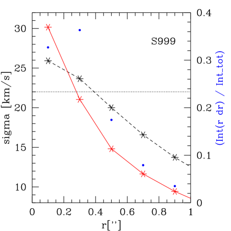
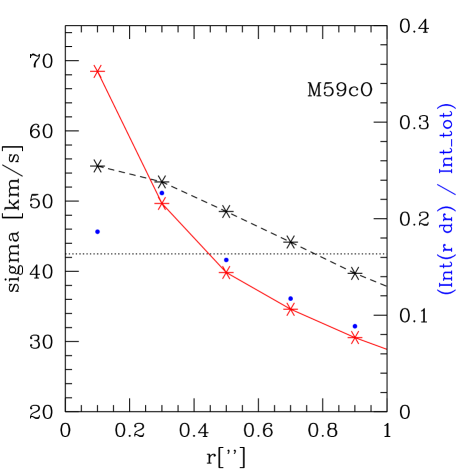
Figure 8: Expected velocity dispersion profile for the two UCDs with the highest predicted BH masses. Left panel: Virgo UCD S999 (Haşegan et al. 2005), for which a central BH of $\sim 2.5\times$ 10${}^{7}\rm\,M_{\odot}$ is predicted. Right panel: Virgo UCD M59cO (Chilingarian & Mamon  2008), for which a central BH of $\sim 5\times$ 10${}^{7}\rm\,M_{\odot}$ is predicted. In both plots, the assumed spatial resolution is 0.2^′′, corresponding to the typical resolution possible in ground based AO assisted spectroscopy. The measured global velocity dispersion is indicated by the horizontal dotted line. The dashed (black) line is the velocity dispersion profile that reproduces the observed global velocity dispersion for the assumption of a uniformally distributed dark mass component on top of the photometric mass. The solid (red) line is the velocity dispersion profile that reproduces the observed global velocity dispersion for the assumption of a central point mass on top of the photometric mass. The small (blue) dots indicate the fraction of light from the source that is contained within each ring around the indicated values of r, with the right y-axis showing the scale.

5 Conclusions and Outlook

Massive UCDs ($\rm M>10^{7}\rm\,M_{\odot}$) have elevated dynamical M/L ratios compared to expectations from stellar population models, with an average ratio $\Psi=(M/L)_{\rm dyn}/(M/L)_{\rm pop}=1.7\pm 0.2$. This implies notable amounts of dark mass in them.

We find that, on average, central BH masses of 10-15% of the UCD mass can explain these elevated dynamical M/L ratios of UCDs, with individual BH masses between 10${}^{5}\rm\,M_{\odot}$ and several 10${}^{7}\rm\,M_{\odot}$ (Fig. 4). In the $M_{\rm BH}-$Luminosity plane, UCDs are offset by a factor of $\sim$100 in BH mass from the relation defined by galaxies (Fig. 6).

These findings fit well to the scenario that massive UCDs are tidally stripped nuclei of originally much more massive galaxies, and their putative central black holes are a fossil relict of their progenitor:

• The estimated BH mass fractions of 10-15% agree with those found in present-day nuclei of galaxy bulges (Fig. 5) that have the masses expected for UCD progenitor galaxies (M$\sim$$10^{9}\rm\,M_{\odot}$; Bekki et al. 2003, Pfeffer & Baumgardt 2013).

• The factor 100 offset to the $M_{\rm BH}-$Luminosity relation would suggest UCD progenitor masses M$\sim$$10^{9}\rm\,M_{\odot}$, again consistent with expectations within the tidal stripping scenario.

The elevated dynamical M/L ratios of UCDs are most prominent for UCD masses above $\sim$$10^{7}\rm\,M_{\odot}$, which corresponds to $\lesssim 10\%$ of the overall UCD population. This relatively small fraction is consistent with the finding that the overall number of UCDs matches well the extrapolated globular cluster luminosity function (Mieske et al. 2012). We also find tentative evidence for a bimodal $\Psi$ distribution in low-mass UCDs ($2\times 10^{6}<\rm M<10^{7}\rm\,M_{\odot}$), suggestive of an overlap of globular clusters and tidally stripped nuclei in this regime.

From these findings a picture of two UCD formation channels emerges: a ’globular cluster channel’ important mainly for UCDs with $M\lesssim 10^{7}\rm\,M_{\odot}$; and, tidal transformation of massive progenitor galaxies which dominates for UCDs $M\gtrsim 10^{7}\rm\,M_{\odot}$ and still contributes for lower UCD masses.

We re-iterate that a massive BH as relict tracer of a massive progenitor is of course only one possibility to explain the elevated M/L. Other scenarios include a globally different IMF (Mieske & Kroupa 2008; Dabringhausen et al. 2012), or highly concentrated dark matter (Haşegan et al. 2005, Goerdt et al. 2008, Baumgardt & Mieske 2008).

The next step in assessing the plaubsility of the BH scenario are more direct observational tests. One clear possibility is to measure spatially resolved velocity dispersion profiles. As noted in the Introduction, a first such measurement was presented for the Fornax UCD3 by Frank et al. (2011), based on IFU observations at very good natural seeing (0.5-0.6$"$ resolution). In that investigation, no indication for the characteristic expected rise of the velocity dispersion profile at small radii was detected. Due to its large intrinsic size of $\sim$1$"$, UCD3 is one of the very few UCDs suited for such natural seeing tests. However, at the same time it is one of the UCDs whose dynamical M/L are fully consistent with a canonical stellar population without a BH (Table LABEL:tableall).

Therefore, observational efforts should now focus on adaptive optics assisted spectroscopy with higher spatial resolution, to be able to target also those UCDs with smaller intrinsic sizes $\lesssim 0.5"$. In Fig. 8 we show the predicted velocity dispersion profiles for the two UCDs with highest predicted BH masses, S999 and M59cO in Virgo, assuming a spatial resolution of 0.2$"$. From the plots one can distill the obervational requirement to distinguish between the profile with a central BH of the predicted mass and a mass-follows-light case. Three independent radial measurements out to $r\sim 0.5"$ would require a precision $\Delta\sigma\sim$ 5 km/s at $\sigma=$20 km/s for S999, and $\Delta\sigma\sim$ 10 km/s at $\sigma=$50 km/s for M59cO. Especially for M59cO this is feasible with current instrumentation, e.g. LGS IFU spectropscopy using NIFS@GEMINI or SINFONI@VLT. In Fig. 8 we also indicate the fraction of the total flux which is contained in each ring around a given r, based on the literature surface brightness profile and an assumed spatial resolution of 0.2$"$ achievable with adaptive optics. For the innermost three radial bins up to $r\sim 0.5"$, the flux per bin is relatively constant, and only drops for larger radii. A direct observational detection of BH signatures thus seems possible for the most emblematic UCDs.

Another possibility for BH detection in UCDs is to analyse their X-ray and Radio emission, looking for the signatures typical for the accretion onto BHs (e.g. Gallo et al. 2003). Several recent studies have reported evidence for stellar mass or intermediate mass black holes in globular clusters and dwarf galaxies from such analyses (e.g. Maccarone et al. 2007, Farrell et al. 2009, Strader et al. 2012& 2013; but see also Maccarone et al. 2008), which makes a systematic survey in the UCD regime an interesting prospect.

We conclude that central BHs as relict tracers of massive progenitors are a plausible explanation for the elevated dynamical M/L ratios of massive UCDs (M$\gtrsim 10^{7}\rm\,M_{\odot}$).