Filter Induced Bias in $\rm{Ly\alpha}$ Emitter Surveys:
A Comparison Between Standard and Tunable Filters.
Gran Telescopio Canarias Preliminary Results

Abstract

$\rm{Ly\alpha}$ emitter (LAE) surveys have successfully used the excess in a narrow-band filter compared to a nearby broad-band image to find candidates. However, the odd spectral energy distribution (SED) of LAEs combined with the instrumental profile have important effects on the properties of the candidate samples extracted from these surveys. We investigate the effect of the bandpass width and the transmission profile of the narrow-band filters used for extracting LAE candidates at redshifts $z\simeq 6.5$ through Monte Carlo simulations, and we present pilot observations to test the performance of tunable filters to find LAEs and other emission-line candidates. We compare the samples obtained using a narrow ideal-rectangular-filter, the Subaru NB921 narrow-band filter, and sweeping across a wavelength range using the ultra-narrow-band tunable filters of the instrument OSIRIS, installed at the 10.4 m Gran Telescopio Canarias. We use this instrument for extracting LAE candidates from a small set of real observations. Broad-band data from the Subaru, HST and Spitzer databases were used for fiting SEDs to calculate photometric redshifts and to identify interlopers. Narrow-band surveys are very efficient to find LAEs in large sky areas, but the samples obtained are not evenly distributed in redshift along the filter bandpass, and the number of LAEs with equivalent widths $<60$ Å can be underestimated. These biased results do not appear in samples obtained using ultra-narrow-band tunable filters. However, the field size of tunable filters is restricted because of the variation of the effective wavelength across the image. Thus narrow-band and ultra-narrow-band surveys are complementary strategies to investigate high-redshift LAEs.

1 Introduction

The odd spectral energy distribution of $\rm{Ly\alpha}$ Emitter Galaxies (LAEs) convolved with the instrumental profile can introduce unsought biases on the characteristics of the candidate samples extracted from photometric surveys. Particularly, properties such as the the Equivalent Width (EW) and the redshift distribution of the subsequently spectroscopically confirmed LAEs, may be easily affected by the photometric survey instrumentation and methodology used. On the other hand, these surveys yield reliable photometric redshifts for LAEs and Lyman Break Galaxies (LBGs), and thus they are useful cosmological tools, as these objects trace dark matter halos and subsequently the evolution of matter distribution in the universe. Furthermore, LAEs at $z\geq 6.5$ are also important to study the last stages of the reionization epoch (Malhotra & Rhoads, 2004; Kashikawa et al., 2006; Shibuya et al., 2012). Therefore, it is important to develop unbiased alternative strategies to find new LAE candidate samples.

LBG candidates are selected using the drop-out technique, which consists in comparing images of the galaxy obtained in several broad-band filters that cover contiguous wavelength ranges to both sides of the Lyman break at 912 Å (Steidel et al., 1996). In a similar way, LAE candidates are usually selected by an excess in a narrow-band filter compared to a nearby broad-band image (Cowie & Hu, 1998). The later technique is routinely used to find LAE candidates in the Subaru Deep Field (Taniguchi et al., 2005; Kashikawa et al., 2006, 2011) and the Subaru/XMM-Newton Deep Survey Field (Ota et al., 2010; Ouchi et al., 2010; Shibuya et al., 2012). Narrow-band filters have bandwidths of Full Width at Half Maximum FWHM $\sim$ 100 Å, and to avoid atmospheric OH emission-lines, narrow-band surveys are confined to a limited number of redshift ranges. An important result of the narrow-band surveys is that the luminosity function of LAEs remains constant between redshifts $3.0\leq z\leq 5.7$, but evolves dramatically between $5.7\leq z\leq 6.5$, and maybe beyond (Pentericci et al., 2011; Hibon et al., 2012; Ota & Iye, 2012).

Despite the utility of narrow-band filters to find LAE candidates, some groups have used ultra-narrow-band filters to perform this task. Thus, Tilvi et al. (2010) and Krug et al. (2012) have employed a filter with a FWHM $\sim$ 9 Å, installed on the 4 m Mayall Telescope, seeking LAEs at redshift $z=7.7$; they expected to find one or two LAEs, respectively, but instead found four LAE candidates, and argued about a possible lack of evolution of the LAE LF for redshifts from 3.1 to 8. Recently, Swinbank et al. (2012) searched for LAEs around two quasars at $z\sim 2.2$ and one quasar at $z\sim 4.5$ with the Taurus Tunable Filter instrument installed on the 3.9 m Anglo-Australian Telescope, using a bandpass of FWHM $=$ 10 Å, and found a local number density an order of magnitude higher than what might be expected in the field.

The spectra of LAEs are characterized by an asymmetric $\rm{Ly\alpha}$ line profile with a steep blue cutoff due to absorption by neutral hydrogen, as shown in Figure 3 in Hu & Cowie (2006). At redshifts $z>6$, hydrogen completely suppresses the continuum of the galaxy at the blue side of the line (Gunn-Peterson trough), while there is a dim continuum at the red side. Narrow band selected LAEs usually have high line luminosities ($L_{\alpha}>1.5\times 10^{42}\,\rm{erg\,s^{-1}}$) and large line equivalent widths at rest ($EW_{0}\geq 20$ Å, e.g. Dayal & Ferrara, 2012; Mallery et al., 2012), although the actual limits may substantially vary because of technical constraints and selection strategies (cf. Hayes et al., 2010; Ouchi et al., 2008, 2010). These properties provide clues which suggest that LAEs represent an early stage of a starburst in an interstellar medium of very low metallicity and almost free of dust, with a radius of about 2 kpc and star formation rates around 6 M_⊙ yr^-1 (Taniguchi et al., 2005).

The fraction of $\rm{Ly\alpha}$ photons that escape from a high-redshift star forming region is still an active and open topic, as well as an important parameter to account for the observable properties of LAEs. Neutral hydrogen resonantly scatters the $\rm{Ly\alpha}$ photons, changes their escape paths and hinders the realization of the photons that are absorbed by dust. Ono et al. (2010) place an upper limit of 20% escaping photons at $z=6.6$, but at lower redshifts Blanc et al. (2011) and Ciardullo et al. (2012) find that the photon escape fraction may be as high as 100%. Hayes et al. (2010) consider the $\rm{Ly\alpha}$ luminosity density at $z=2$ significantly underestimated from its intrinsic value, due to the fact that only 1 in 20 photons, on average, reach the telescope; this will specially happen at $z>6$, where the neutral fraction of the intergalactic medium may cause significant suppression of the $\rm{Ly\alpha}$ line (Santos et al., 2004; Hayes & Östlin, 2006; Dijkstra et al., 2007). On the other hand, $\rm{Ly\alpha}$ photons may be less attenuated than non-resonant radiation under suitable conditions within a multiphase scattering medium (Neufeld, 1991; Hansen & Oh, 2006; Finkelstein et al., 2008). For Finkelstein et al. (2011), dust geometry shapes the spectral energy distributions, and has a major influence in the observed EW at the rest frame of the $\rm{Ly\alpha}$ line ($EW(\rm{Ly\alpha})$) distribution in high-redshift LAEs. Finally, the presence of outflows can increase the fraction of $\rm{Ly\alpha}$ photons that escape from the star forming region (Kunth et al., 1998; Tapken et al., 2007; Verhamme et al., 2006, 2008; Atek et al., 2008, 2009).

If the observational aspects of LAEs depend on geometrical effects (dust spatial distribution), orientation, and the presence of outflows, the separation between LBGs and LAEs becomes somewhat diffuse. Thus, Kashikawa et al. (2007) classify galaxies with contrasts as low as $EW(\rm{Ly\alpha})>10$ Å as LAEs, while recently Krug et al. (2012) consider even lower limits ($EW(\rm{Ly\alpha})\gtrsim 4.8$ Å) for $z\sim 7.7$ LAEs. Besides, other observations indicate that the fraction of low ultraviolet luminosity LBGs ($M_{\rm{UV}}>-20.5$) with $EW(\rm{Ly\alpha})>50$ Å is about one half (Stark et al., 2010, 2011; Pentericci et al., 2011; Schenker et al., 2012; Vanzella et al., 2011; Ono et al., 2012). The presence of $\rm{Ly\alpha}$ lines in some LBGs provides a strong evidence of the connection between these objects and LAEs. Eventually, this connection will promote an effort to build theoretical models to explain the underlying physics of LAEs and LBGs (e.g Shapley et al., 2001; Dayal & Ferrara, 2012; Forero-Romero et al., 2012).

We are conducting a blind search on selected gravitationally lensing galaxy cluster sky fields to obtain samples of LAEs not subjected to possible biases imposed by the methodology of narrow-band filters. Hence, we are obtaining ultra-narrow-band images using tunable filters of the instrument OSIRIS (OSIRIS-TF) attached to the 10.4 m Gran Telescopio Canarias (GTC). OSIRIS-TF is optimized for line flux determination and thus it can be called a Star Formation Machine (Cepa et al., 2003). This characteristic makes OSIRIS-TF a powerful instrument to detect faint young galaxies with accurate photometric redshift estimates. Therefore, apart from LAEs, we also expect to obtain other high-redshift candidates, such as LBGs, AGNs and line emitters.

This paper is organized as follows. Section 2 introduces the bias produced by the filter bandwidth on the photometric selection of LAEs. Section 3 describes the generation of Monte Carlo data for simulated LAE spectra. Section 4 presents the LAE recovered samples obtained using narrow-band filters on the simulated data, exemplified by an ideal rectangular filter and the NB921 Subaru filter. Section 5 describes the methodology used to search for LAE candidates using OSIRIS-TF, and presents the sample recovered from the simulated data. Our methodology is then applied on a pilot observation of real data obtained at the GTC to select preliminary candidates at redshifts $z\simeq 6.5$. In Section 6 we cross-check our OSIRIS-TF preliminary candidates with photometric archive data and models of galaxies at high redshift to study the Spectral Energy Distribution (SED) and to improve classification. Section 7 presents the discussion of the results obtained with simulated and real data. Finally, Section 8 presents our conclusions.

Throughout this paper we assume a cosmological model with $H_{0}=70\,\mathrm{km\,s^{-1}\,Mpc^{-1}}$ ($h=0.7$), $\Omega_{\rm{M}}=0.27$, and $\Omega_{\Lambda}=0.73$.

2 The asymmetric continuum bias

The spectrum of a LAE at $z\sim 6.5$ shows a sharp decay due to the absorption of $\rm{Ly\alpha}$ photons by neutral hydrogen that truncates the blue part of the emission line. From the observational point of view the resulting line is asymmetric, and the signal is circumscribed to wavelengths longer than $\rm{Ly\alpha}$.

The detection of dim objects is a difficult task and very often the results may vary depending on subtle details. In the case of LAEs, the spectral asymmetry of the host galaxy continuum background with respect to the $\rm{Ly\alpha}$ line may enhance the detection of objects with the largest contribution of the continuum to the total signal. If we use a narrow-band filter with a FWHM comparable to the EW of the $\rm{Ly\alpha}$ line, the contribution of the continuum to the total recorded intensity may change significantly depending on the redshift of the object. Figure 1 shows an example of this effect on an ideal rectangular filter of a width of 132 Å, similar to the FWHM of the NB921 Subaru filter. The figure shows two simplified LAE spectra at slightly different redshifts (6.51 and 6.61). The objects have an observed FWHM of 10 Å for the $\rm{Ly\alpha}$ line, and an identical continuum level. For the LAE at the lowest redshift, the $\rm{Ly\alpha}$ line lies on the short-wavelength edge of the filter, and its EW is 2.5 times the wavelength range of the filter (i.e., 330 Å in the observer’s frame or 44 Å in the rest-frame), which corresponds to a difference of one magnitude between the line and the continuum, a criterion often used to select LAE candidates in narrow-band surveys (e.g. Ouchi et al., 2010; Kashikawa et al., 2011). For the LAE at the highest redshift, to reach the same signal through the rectangular filter, the intensity of the $\rm{Ly\alpha}$ line (or its EW) should be approximately 34% higher than the line intensity of the former object.

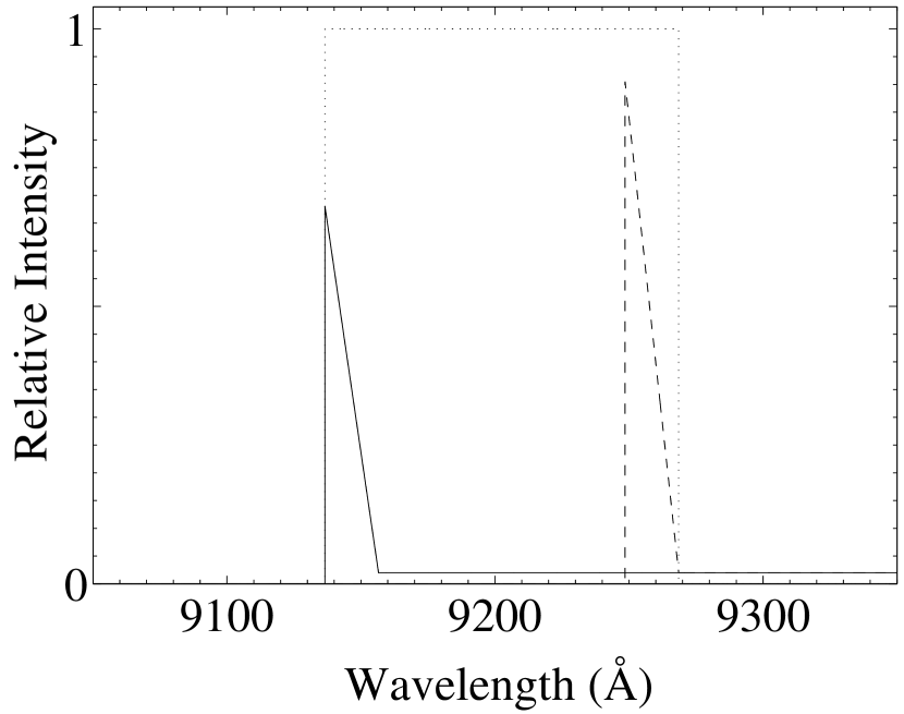
Figure 1: An example of the effect of the asymmetric continuum in the detection of LAEs. The amount of the continuum inside the ideal rectangular filter (dotted line) depends on the position of the $\rm{Ly\alpha}$ break. In the extreme cases shown in this diagram, the continuum expands on the whole wavelength range of the filter for objects at the lowest redshift (solid line) or barely in the region covered by the $\rm{Ly\alpha}$ line for objects at the highest redshift (dashed line). Both objects share the same continuum level and the observed FWHM of the $\rm{Ly\alpha}$ lines is 10 Å. For the object at the lower redshift, the contribution of the $\rm{Ly\alpha}$ line is 2.5 that of the continuum in the range of the filter. For detecting the highest redshift object with the same total signal, the $\rm{Ly\alpha}$ line must be approximately 34% more intense than the line of the lower redshift object.

The bias introduced by the asymmetric continuum profile at both sides of the $\rm{Ly\alpha}$ line is more pronounced as the EW decreases. The observed-frame EW for LAEs have values $\sim 100$ Å, similar to a narrow-band filter FWHM. Therefore, the asymmetric continuum may affect the shape of the LF of LAEs inferred from narrow-band surveys. As objects are less luminous, the volume actually studied depends on the amount of continuum in the range of the filter.

3 Sample simulation

Shimasaku et al. (2006) and Ouchi et al. (2008) have analyzed the redshift distribution of LAEs in Subaru’s narrow-band filters using Monte Carlo mock samples of LAEs. For the purpose of comparing the characteristics of samples obtained with the OSIRIS-TF and other instruments, we have also built a simulated sample of LAEs. This sample was made by modeling the LAE spectra with a superposition of an asymmetric triangular profile for the $\rm{Ly\alpha}$ line plus a continuum, which is a simplified version of the profile model by Hu et al. (2004). The $\rm{Ly\alpha}$ line profile consists of a sawtooth with the steeper inclination at the line’s blue side. At wavelengths shorter than the $\rm{Ly\alpha}$ line, the continuum is zero, and it has some constant non-zero value at wavelengths equal or larger than the $\rm{Ly\alpha}$ line. Altogether, we have simulated the spectra of 5000 LAEs.

We have used the Schechter function to model the LF of LAEs at $z\simeq 6.5$:

$$\phi={\phi_{*}}\left({\frac{L}{{{L_{*}}}}}\right)^{\alpha}\exp{\left({\frac{-L}{{{L_{*}}}}}\right)}\,\frac{{dL}}{{{L_{*}}}},$$ (1)

with the parameters given by Kashikawa et al. (2011): $\alpha=-1.5$, $\log(L_{*}/h^{-2}\,\mathrm{erg\,s^{-1}})=42.76$ and $\log(\phi_{*}/h^{3}\,\mathrm{Mpc^{-3}})=-3.28$.

The simulated LF sample was computed through the inversion method of the cumulative Schechter function, integrating between $10^{41}$ and $10^{44}$ $\,\rm{erg\,s^{-1}}$, a luminosity range that broadly includes the observed LAEs at redshifts $z\approx 6.5$ (e.g. Kashikawa et al., 2011).

A random FWHM sample for the $\rm{Ly\alpha}$ line has been computed according to the distribution parameters inferred from Table 2 in Kashikawa et al. (2011). These authors have measured the observed FWHM of 28 $z\approx 6.5$ LAEs with values between 5.04 Å and 25.2 Å, with mean of 13 Å (428 km s^-1) and a standard deviation of 5 Å. The FWHM sample has been shifted to the rest-frame of the LAEs to build the profile of the emitted $\rm{Ly\alpha}$ line.

The random EW sample at rest-frame ($EW_{0}$) has also been computed like the luminosity, using the inversion method on the cumulative function extracted from Figure 11 in Kashikawa et al. (2011). We tried to fit the EW distribution using exponential cumulative functions, but we obtained a better fit using the lognormal cumulative function. Lognormal EW distributions also fit the [O II]_λ3727 equivalent widths in the local ($z<0.2$) universe (Blanton & Lin, 2000), and has been employed by Shimasaku et al. (2006) to characterize the EW of LAEs at redshift ($z\simeq 5.7$). However, the $\rm{Ly\alpha}$ EW distribution in LBG at $z\sim 3$ does not show lognormal profile (Shapley et al., 2003), possibly because in LBGs $\rm{Ly\alpha}$ is observed both in emission and in absorption, depending on the object. In any case, accurate EW measurements are difficult mainly because of the low level of the galaxy continuum, and thus the actual shape of the $\rm{Ly\alpha}$ EW distribution is still an open subject. The $EW_{0}$ in our simulations has a median value of 68 Å, slightly below the value of 74 Å reported by Kashikawa et al. (2011). By construction, the lower values of the simulation were restricted to $EW>0$. Extreme values are useful to test the instrumental response and to set constraints to the distribution of real objects. If the simulations show that the instrument reaches a certain parameter or combination of parameter values, but the corresponding objects have not been observed, it is evidence that there are few if any of them. On the other hand, if the simulations show that the instrument cannot detect objects with certain combinations of parameter values, it remains an open question whether these objects exist or not. In any case, because the simulation is based on empirical parameter distributions, extreme values are very improbable, and they cannot significantly alter the statistical results of this study. For example, in our simulation we find 69 objects with $EW_{0}<8$ Å, and 77 with $EW_{0}>600$ Å from 2708 OSIRIS-TF recovered LAEs; of course these numbers depend on the EW distribution adopted, which may be critical for the low EW regime.

To set thresholds for the EWs of LAEs is not a simple task. In some cases the continuum may be undetected, and the maximum threshold cannot be determined. In the case of the minimum threshold, Stark et al. (2010) have proposed that the equivalent width at the rest frame should be $EW_{0}>55$ Å for LAEs. More recently, these authors have proposed a value of 25 Å (Stark et al., 2011) that approaches the widely accepted minimum threshold of $EW_{0}>20$ Å. The intensity of the $\rm{Ly\alpha}$ line and its EW may depend on intrinsic properties of the LAEs or on geometrical attributes (see § 1). Moreover, the adopted threshold is a figure that probably depends also on the observational limits adopted to separate candidates efficiently. Thus, Stark et al. (2011) note that the measured rest-frame EWs of the $\rm{Ly\alpha}$ line for 13 spectroscopically confirmed LAEs range between 9.4 Å and 350 Å. Therefore, we have conserved even the most extreme values for the EW in our simulations. Besides, these values may be useful to make extreme-case differences between the respective methodologies to detect LAE candidates.

For each simulated LAE, once the power of the $\rm{Ly\alpha}$ line ($L_{\rm{Ly\alpha}}$) and its $EW_{0}$ have been assigned, it is possible to calculate the spectral power $\Phi_{c}$ of the continuum:

$$\Phi_{c}=\frac{L_{\rm{Ly\alpha}}}{EW_{0}}.$$ (2)

This spectral power is used to compute the spectral shape of the continuum at wavelengths $\lambda\geq\lambda_{\rm{Ly\alpha}}$. For wavelengths $\lambda\leq\lambda_{\rm{Ly\alpha}}$, the continuum is assumed to be zero, as the optical depth for photons with wavelengths shorter than the $\rm{Ly\alpha}$ line is large. Equation (2) is also used to build a continuum of reference for all the wavelengths of interest in our analysis, which will be used later to estimate a broad-band continuum emission necessary for the criterion of detection.

The observed spectra for both, the $\rm{Ly\alpha}$ line and the continuum, have been calculated from the corresponding spectral luminosities taking into account the redshift for each simulated object. These lines and continuum spectra have been added in order to obtain the observed flux, from which we will get the photometry later in our analysis. We have constructed another spectrum of constant intensity for each object, calculated from the corresponding continuum of reference.

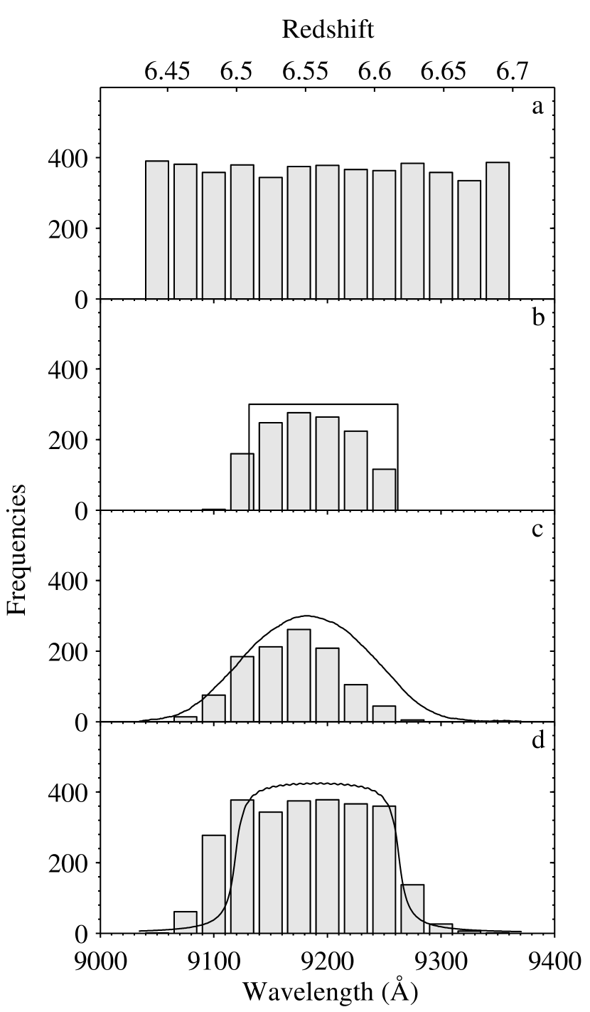
Figure 2: Number of simulations and detections. Panel (a) shows the absolute frequency per wavelength bin of the simulated population of LAEs. Panels (b) and (c) depict the number of detections computed for an ideal rectangular filter and for the Subaru NB921 filter; both panels show the transmission profile for the respective filter superposed. Panel (d) renders the number of detections computed for the OSIRIS-TF, along with the transmission profile of the wide filter (solid line) built using the band synthesis technique (see text).

4 Narrow-band filters

In this section we analyze the outcome produced by narrow-band filters applied to our simulated sample. Gronwall et al. (2007) have noted the effect of a nonsquare bandpass in the definition of survey volume and sample’s flux calibration for large photometric selected samples of emission-line galaxies. For these authors, the volume of space sampled is a strong function of line strength: objects with bright line emission can be detected even if the $\rm{Ly\alpha}$ line lies in the wings of the filter, but for weak $\rm{Ly\alpha}$ sources the line must lie near the bandpass center to be noticeable. Furthermore, ignoring the actual position of the line in the bandpass prevents a precise estimate of the effective filter transmission in the line position, affecting the flux calibration. Being aware of these constraints, we consider two narrow-band filter profiles. First, an ideal rectangular filter to study the effect of a general pass-band filter on the detection of LAEs, and secondly a filter with a response similar to that of Subaru NB921 attached to the Suprime-Cam, to study the effect of a real-life filter profile.

Figure 2 shows the distribution of the simulated sample, the ideal and the NB921 Subaru filters, and the OSIRIS-TF (see §5). The simulations yield a number of approximately 400 objects per wavelength bin (each bin with a width of 25 Å).

4.1 Ideal rectangular filter

The ideal rectangular filter is defined such as:

$$T_{\lambda}=\begin{cases}1&\text{if }9130\leq\lambda\leq 9262\,\text{\AA},\\ 0&\text{otherwise,}\end{cases}$$ (3)

where $T_{\lambda}$ is the transmission of the filter as a function of the wavelength $\lambda$. The bandwidth of the filter defined above is 132 Å, which equates the FWHM of the Subaru NB921 filter (see § 4.2).

Simulated LAEs are recovered according to two criteria, one for source detection and the other for LAE candidate discrimination. The detection criterion is fulfilled when the irradiance in the narrow-band filter is $\geq 5\times 10^{-18}\,\,\rm{erg\,s^{-1}\,cm^{-2}}$, which corresponds to the Subaru flux limit (Ouchi et al., 2010). The discriminant criterion is a contrast condition between the narrow-band and the broad-band fluxes. This criterion is in fact a simplified version of the Ouchi et al. (2010) color criterion, but is sufficient to analyze the simulated data. In our case, the condition that must be accomplished consists of the narrow-band flux being at least a magnitude brighter than the (adjacent) broad-band flux, which provides a continuum of reference. Computationally, this criterion leads to the flux of the object measured through the filter being at least 2.5 times larger than the flux measured from the constant continuum of reference computed in § 3.

Results are shown in Figure 2b. Roughly, due to the asymmetric continuum bias, a larger number of detections at shorter wavelengths are expected, and decays smoothly at longer wavelengths. Small departures from this behavior are due to random deviations in the original simulated sample redshift distribution. Thus, most detections are scattered over the filter pass-band, but some simulated objects with their $\rm{Ly\alpha}$ peaks lying at shorter wavelengths are recovered.

Only around a fourth part of the wavelength range in the leftmost bin in Figure 2b lies inside the filter profile, and almost half of the recovered objects in this bin correspond to simulations with the $\rm{Ly\alpha}$ line peak located inside the filter pass-band. In fact, most recovered objects in this bin (83 out of 160) have the peak of the $\rm{Ly\alpha}$ line at wavelengths shorter than the filter window, but with a fraction of the long wavelength queue of this line inside the filter. Note that the detection of these objects will depend on the line parameters (peak position, FWHM and intensity), and that the recorded signal will be diminished by the loss of the line flux outside the filter window, and thus these objects tend to have larger EWs that make detections easier. On the other hand, the smooth decay of the number of recovered LAEs along the filter pass-band is a result of the smaller quantities of the continuum emission lying inside the filter as the $\rm{Ly\alpha}$ line peaks at longer wavelengths. For objects with their $\rm{Ly\alpha}$ line near the long wavelength extreme of the filter, the contribution of the continuum to the total flux in the band is negligible, and part of the long wavelength queue of the line may also lie outside the filter window, yielding a steep drop in the number of detections. Therefore these objects also tend to have large EWs to compensate for their total loss of flux.

4.2 Subaru filter

NB921 filter is characterized by an almost Gaussian profile with a central wavelength at 9196 Å and a FWHM of 132 Å (Kashikawa et al., 2011), that corresponds to a spectral resolution of 70. The transmission profile is available from Subaru.​ A close inspection of this profile shows that the maximum of the recovered LAEs is slightly offset (9183 Å) with respect to the filter peak, in agreement with the $\rm{Ly\alpha}$ wavelength distribution of confirmed LAEs reported by Kashikawa et al. (2011).

We used the same detection criteria as in the case of the ideal rectangular filter. The results are shown in Figure 2c. The number of recovered LAEs is restrained by the filter profile along with the same effects that have been noted in the ideal rectangular filter. On the one hand there is the decay of the continuum contribution for the objects with the peak of the $\rm{Ly\alpha}$ line closer to the long wavelength limit of the filter, on the other hand there also is the loss of the long wavelength queue of the $\rm{Ly\alpha}$ line, which spreads to the low transmission region of the filter profile. Therefore, the long wavelength queue of the line observed through the Subaru filter is damped by the bell-shaped transmission, in agreement with Shimasaku et al. (2006) and Ouchi et al. (2008).

5 Tunable filters

Throughout this work, a distinction is drawn between a frame, corresponding to one set of data read from the CCDs; an image, a number of frames at the same etalon settings which have been combined for analysis; a field, a stack of images of the same area of sky at different etalon settings.

5.1 OSIRIS tunable filters

Basically, the imager/spectrograph OSIRIS-TF is a low resolution Fabry-Pérot spectrograph which consists of a blue and a red arm. Our observations were performed with the red arm, that can be centered at any wavelength between 6500 and 9300 Å, and we observed using a fixed bandpass of 12 Å which corresponds to a spectral resolution of about 770, a set of order-sorter filters to avoid contamination by neighboring orders, and a detector array consisting of two MAT 4k$\times$2k CCDs (Cepa et al., 2003). The 12 Å  bandpass is the only one currently available for wavelengths around 9200 Å.

The observing strategy consists on sweeping a selected spectral range using steps of a half of the FWHM (in our case, 24 images shifted 6 Å between 9122 and 9260 Å) to avoid aliasing. To apply this methodology to our simulated data, we have modeled a set of 24, approximately Lorentzian shaped, tunable filters using the following approximation that relates wavelengths and transmissions of the OSIRIS-TF (Cepa et al., 2011, eq. 3.14):

$$T\approx\Bigg{\{}1+\left[\frac{2(\lambda-\lambda_{0})}{\delta\lambda}\right]^{2}\!\Bigg{\}}^{-1}\!\!\!\!\!\!,$$ (4)

where $\delta\lambda$ is the filter FWHM and $\lambda_{0}$ is the central wavelength.

Figure 3 shows a simulated LAE at redshift $z=6.6$ (a), the set of OSIRIS-TF filtered spectra for this simulation (b), and the photometric output (c). This particular simulation has a rather small $EW_{0}=17.8$ Å, which is adequate to make the continuum more apparent in the plot. In panel (c), the short wavelength edge of the line aliases because the spectrum varies at a higher frequency than the OSIRIS-TF spectral resolution. Nonetheless, the asymmetry of the line profile is still noticeable.

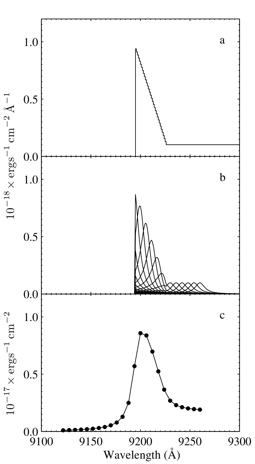
Figure 3: OSIRIS-TF output. Panel (a) shows the spectral flux density of a LAE at $z=6.6$ simulated spectrum. Panel (b) shows the set of OSIRIS-TF transmitted spectra for this simulation. Panel (c) renders the photometric output for each OSIRIS-TF, which is the signal integrated over each filter. Note that the units and the scale of the last plot are different from the two previous diagrams.

In this paper we have adopted two criteria to retrieve LAEs from the simulations, based on the characteristics of OSIRIS-TF. The first is a detection condition that imposes an irradiance $\gtrsim 4\times 10^{-18}\,\,\rm{erg\,s^{-1}\,cm^{-2}}$ for the field narrow-band image. This field is built through the sum of the 24 ultra-narrow-band filters to provide a wider synthetic filter (band synthesis technique, Cepa, 2009). The second condition consists of a ratio between the maximum and minimum of the 24 filters larger than 2.5 (i.e., one magnitude). These conditions are equivalent to those imposed to the Subaru survey.

Table 1: High redshift OSIRIS-TF candidates

ID	RA			DEC			Redshift	Irradiance		Candidates
	hh:mm:ss.s			dd:mm:ss						OSIRIS-TF only	OSIRIS-TF & SED
$\mathbb{A}$a	20:	56:	23.8	-4:	40:	07	6.494	4.01 $\pm$	0.09	LAE	Interloper / [O II]  emitter
$\mathbb{A}$b	20:	56:	25.0	-4:	37:	07	6.498	1.05 $\pm$	0.09	LAE	LBG
$\mathbb{A}$c	20:	56:	23.8	-4:	37:	02	$\lesssim$6.494	1.12 $\pm$	0.09	LAE	Interloper / [O II]  emitter
$\mathbb{B}$a	20:	56:	38.1	-4:	40:	04	$\gtrsim$6.448	1.49 $\pm$	0.09	LAE/LBG	Interloper
$\mathbb{B}$b	20:	56:	26.4	-4:	37:	14	$\gtrsim$6.512	1.67 $\pm$	0.09	LAE/LBG	Interloper / [O II]  emitter
$\mathbb{C}$a	20:	56:	16.7	-4:	37:	53	6.513	1.00 $\pm$	0.09	LBG	Young spiral galaxy
$\mathbb{C}$b	20:	56:	30.6	-4:	37:	37	6.502	1.82 $\pm$	0.09	LBG	LBG

Results are shown in Figure 2d. The distribution of the simulated LAEs recovered using OSIRIS-TF expands the full range of wavelengths between 9122 and 9260 Å. A visual inspection of Figures 2a and 2d shows that the shape of the distribution in this range of wavelengths closely resembles that of the simulated LAEs, without any apparent bias introduced by the filter profiles. Also notice that almost all the simulated objects in this range are recovered. In addition, there also are some retrieved LAEs with their $\rm{Ly\alpha}$ line peak ($\lambda_{\rm{Ly\alpha}}$) outside the 9122 — 9260 Å range, which is a consequence of the OSIRIS-TF Lorentzian profile. These objects tend to have large EWs; and those with $\lambda_{\rm{Ly\alpha}}>9260$ Å tend to be brighter, too.

5.2 OSIRIS-TF pilot observations

Photometry was carried out at the GTC using OSIRIS-TF with FWHM of 12 Å at five contiguous wavelengths separated by steps of 6 Å, and a field of view free of adjacent orders of about 8 arcminutes on each side. The observations were performed with central wavelengths $\lambda_{c}=\text{9122\,{\AA}, 9128\,{\AA}, 9134\,{\AA}, 9140\,{\AA} \& 9146\,{\AA}}$. The observation run was done on 2010 September 8. A binning of $2\times 2$ was used in fast (standard) readout mode (200 kHz), with three dithered exposures per wavelength of 210 s each, and separated by a triangular offset pattern of 10 arcseconds to eliminate diametric ghosts during data reduction, each called a frame. The night was photometric and the seeing varied from 0.75 to 0.82 arcseconds during the observation run.

Following the observation of the cluster in all the wavelengths, a standard star was observed with the same instrumental settings (but different exposure times) for flux calibration.

Standard IRAF procedures for bias subtraction were used on the data. Super-flats (a flat generated by averaging the sky from scientific images where sources have been masked) were created from and divided to the scientific frames due to the unevenly-lit dome flats. Because of the TFs small bandpass and position-dependent wavelength, all observations contain sky (OH) emission rings which were subtracted to all frames with the IRAF package TFred,​ which estimates the sky background, including the sky rings which are several arcminutes in diameter. The three frame offsets of each wavelength were aligned and combined to generate an image with a total exposure time of 630 s, these were later convolved to the worst seeing of 0.82 arcseconds.

Field 0             9122 Å              9128 Å              9134 Å              9140 Å              9146 Å

$\mathbb{A}$a
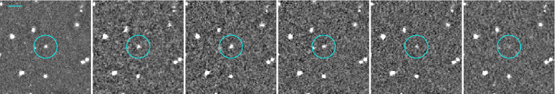
$\mathbb{A}$b
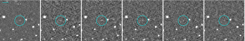
$\mathbb{A}$c
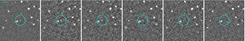
$\mathbb{B}$a
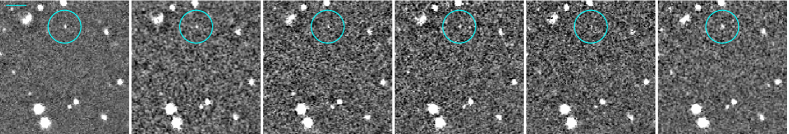
$\mathbb{B}$b
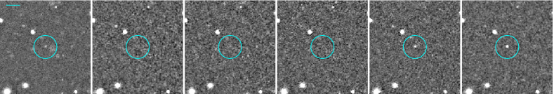
$\mathbb{C}$a
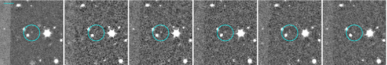
$\mathbb{C}$b

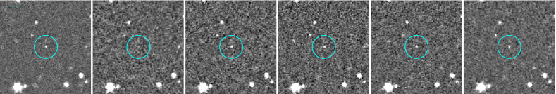
Figure 4: OSIRIS-TF observations. Column 1 shows the field obtained adding five individual images shown in the columns 2–6 labeled by the central wavelength of the tuned filter. The horizontal line at the top left of the fields marks a 6″ scale. Each row corresponds to a different LAE or LBG candidate, identified by the labels at left. The objects lie in the center of the identifying circles.

plain

Also, a field was created convolving to the worst seeing of 0.82 arcseconds, and combining all aligned images of different wavelengths (band synthesis technique). This field has a total integration time of 3150 s, and yields a detection limit irradiance of $9\times 10^{-18}\,\,\rm{erg\,s^{-1}\,cm^{-2}}$ integrated over the full wavelength range (36 Å) of the synthetic band. We used SExtractor (Bertin & Arnouts, 1996) to make a catalog of detected sources in the field. We excluded sources from the catalog that were too bright for high-redshift galaxies. Photometry on each monochromatic image was performed using an aperture of 1.5 arcseconds using the positions gathered by SExtractor. Then we selected possible candidates based on the maximum vs minimum flux ratio, excluding all those sources with a ratio below 2.5 (i.e., one magnitude). The remaining objects were carefully inspected by eye to reject faint cosmic rays, ghost residuals, and source contamination by nearby companions or located too close to the edge of the image; the region around the gap between the detectors was particularly clumped with fake detections. Finally, we selected those candidates that showed a photometric profile similar to those expected for LAEs and LBGs with either the $\rm{Ly\alpha}$ line or the Lyman Break lying, at least partially, inside the observed wavelength range. Given the likely range of Ly$\alpha$ emission-line widths, and the wavelength sampling, we expect to observe this line in more than three adjacent passbands.

Table 1 summarizes the data for the candidates. Column 1 identifies the OSIRIS-TF candidate. Columns 2 and 3 show the right ascension and declination coordinates, respectively. Column 4 shows the redshift obtained from the peak of the alleged $\rm{Ly\alpha}$ line or Lyman break. Column 5 is the total irradiance corresponding to the field. Column 6 and 7 present the classification of candidates obtained using the OSIRIS-TF data, and the SED fitting to Subaru, HST and Spitzer photometrical data.

Figure 4 shows the OSIRIS-TF images for each LAE and LBG candidate. Each row in this figure corresponds to a different object located at the center of a guiding circle. Despite candidate $\mathbb{B}$a being near the upper border of the clipped image, it does not affect our analysis. This is also the case for the candidate $\mathbb{C}$a, which is near the diffuse border defined by the dithered gap between the detectors. The first column of frames in Figure 4 shows the field exposure obtained by piling up all the individual images; the rest of columns show the candidates observed at the wavelength identified in the heading row.

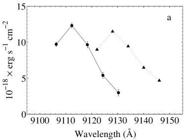
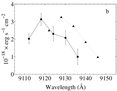
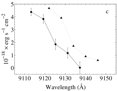
Figure 5: OSIRIS-TF LAE candidates. Panels (a), (b) and (c) correspond to candidates $\mathbb{A}$a, $\mathbb{A}$b, and $\mathbb{A}$c, respectively. Circles connected by solid lines depict OSIRIS-TF photometrical data obtained at the GTC. Triangles linked by dotted lines show examples extracted from our simulations that resemble the real data. Photometrical data are shifted in wavelength with respect to the simulations due to the wavelength dependency of the OSIRIS-TF with the distance to the optical center.

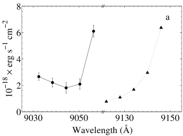
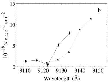
Figure 6: OSIRIS-TF LAE or LBG candidates. The same as in Figure 5, but the spectral profiles are compatible to both LAEs and LBGs. Panels (a), and (b) correspond to candidates $\mathbb{B}$a, and $\mathbb{B}$b, respectively.

Figure 5 shows three LAE candidates observed with the OSIRIS-TF at the GTC, and selected simulations extracted from our database that resembles the real data, rather than a fitted model for each object. The shift in wavelengths between the observations and the model is due to the dependency of the tuned wavelength of the filter on the distance $r$ to the optical center in the OSIRIS-TF images (González et al., 2013, in preparation):

$$\lambda={\lambda_{c}}-5.04{r^{2}}\!\!\!,$$ (5)

where $\lambda_{c}$ is the wavelength at the optical center expressed in Å, and $r$ in arcminutes.

The redshifts for these LAE candidates were calculated identifying the brightest photometric point with the position of the $\rm{Ly\alpha}$ line. For the peak-missed LAE candidate shown in Figure 5c, the redshift estimate is therefore an upper limit (see Table 1). In fact the fraction of candidates with either upper or lower redshift limits are expected to be relatively high. This subject, and the possible contamination of the candidate sample by foreground galaxies, will be addressed in §6 and §7.

The two objects shown in Figure 6 have a photometric profile compatible with either LAE or LBG candidates. Their respective redshift lower limits are shown in Table 1. The photometric profile for the object shown in Figure 6a may be contaminated by residuals of the sky-line subtractions at wavelengths below 9050Å. As in the previous figure, simulated objects extracted from our database are also plotted for comparison purposes.

Objects shown in Figure 7 are two LBG candidates. Both objects show a steep increase in flux that is held at longer wavelengths, as it is expected for the continuum emission of LGBs.

6 Subaru, HST and Spitzer archive data

We have searched for additional photometric data for our LAE and LBG candidates in astronomical public databases, and have found some deep images in the Subaru, Hubble Space Telescope (HST) and Spitzer archives that cover, at least partially, the OSIRIS-TF field around MS 2053.7-0449. We used these data along with our observations to fit the SED of the OSIRIS-TF candidates, obtaining a more accurate classification (see Table 1). Table 2 shows the fluxes in the different bands of Subaru/Suprime–Cam, HST/WPFC2 and Spitzer/IRAC data. This table also includes the fluxes of the OSIRIS-TF band synthesis images, that correspond to a filter of $\rm{FWHM}=36$ Å. In the case of OSIRIS-TF fields and HST fluxes, we found discrepancies based on Subaru calibrations. We then used stars in the field to recalibrate the OSIRIS-TF and HST data to the Subaru photometry.

6.1 Subaru observations

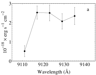
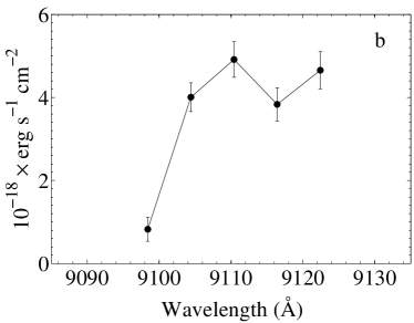
Figure 7: OSIRIS-TF LBG candidates. Panels (a), and (b) correspond to candidates $\mathbb{C}$a, and $\mathbb{C}$b, respectively. Circles with error bars linked by solid lines depict photometrical data obtained with the OSIRIS-TF at the GTC. The spectral profiles are compatible with LBGs.

The Subaru/Suprime–Cam data were obtained from the Subaru-Mitaka Okayama-Kiso Archive System (SMOKA). They consist of data in filters $V$, $i$' and $z$' observed in 2009. The wavelength range of the $z$' filter includes our OSIRIS-TF observations, resulting in a helpful band to estimate the continuum. Data was reduced following the Suprime–Cam Data Reduction software (SDFRED2). The images were flat fielded, matched in PSF size for a predetermined target FWHM, scaled and combined. The total integration time for $V$, $i$' and $z$' filters was 5040, 1920 and 1800 seconds, respectively. The photometry for the candidates was performed with the qphot IRAF package, fluxes were derived by measuring inside a 1.5 arcsecond aperture.

OSIRIS-TF candidates $\mathbb{A}$a, $\mathbb{A}$b, $\mathbb{A}$c and $\mathbb{B}$a are seen in the $V$, $i$' and $z$' filters, pointing at possible interlopers (i.e., a galaxy at a lower redshift and with spectral features resembling those of LAEs over a limited range of wavelengths) or LBG candidates. Candidates $\mathbb{B}$b, $\mathbb{C}$a and $\mathbb{C}$b are not seen in at least one Subaru/Suprime–cam filter, but their best SED fit suggests they are all candidate interlopers.

6.2 HST observations

The HST/WFPC2 data were obtained from the Multimission Archive at the Space Telescope Science Institute (MAST). They consist of two programs: ID5991 (filters F702W and F814W), and ID6745 (filters F606W and F814W). The proposals cover slightly different fields. Only two of the seven candidates fall in the images, namely, $\mathbb{A}$c in the field of the proposal ID5991, and $\mathbb{C}$a in the field covered by ID6745.

The image reduction was performed using the IRAF/STSDASS package. First, a warm-pixel rejection was applied to the images using the IRAF task warmpix. The cleaned images were then combined with the task crrej to remove cosmic-rays hits. Finally, the background was subtracted and the WFPC2 chips were combined using the task wmosaic. The total integration times for filters F702W and F814W were 2400 s and 2600 s, respectively for the proposal ID59991. For the proposal ID6745 the total integration times were 3300 s and 3200 s for filters F606W and F814W, respectively. The photometry for the seven candidates was performed in the HST filters with the IRAF package apphot. The magnitudes were derived by measuring fluxes inside a fixed circular aperture of 7 pixels ($\sim 0\farcs 7$). OSIRIS-TF candidates found in these filters suggest an interloper nature.

6.3 Spitzer/IRAC observations

A Spitzer/IRAC observation was gathered from the Spitzer Heritage Archive (SHA). The Astronomical Observation Request (AOR) number 18626048 (program Name/ID KTRAN-MS2053/30642, P.I. K.-V. Tran) was retrieved for this work. It is a four-channel (3.6, 4.5, 5.8 & 8 $\mu\rm{m}$) IRAC map mode observation consisting of 3 rows and 1 column with a 42-point cycling dither pattern, and “medium” scale (median separation between dither positions is 53 pixels; the IRAC pixel scale is approximately the same, $\sim$ 1.2 arcsec in the four camera bands). The resulting map footprint is a roughly rectangular area of 22.9 $\times$ 8.6 arcmin centered at $\alpha$ $\approx$ 314.113^∘, $\delta$ $\approx$ $-$4.670^∘. The major axis is oriented at P.A. $\approx$ 168.2^∘.

Table 2: Candidate Fluxes

FILTER

$\mathbb{A}$a

$\mathbb{A}$b

$\mathbb{A}$c

$\mathbb{B}$a

$\mathbb{B}$b

$\mathbb{C}$a

$\mathbb{C}$b

Suprime $V$

26$\,\pm\,$

2

$<0.70$

4$\,\pm\,$

1

8.3$\,\pm\,$

0.7

$\cdots$

36$\,\pm\,$

1

$\cdots$

F606W

$\cdots$

$\cdots$

$\cdots$

$\cdots$

$\cdots$

41$\,\pm\,$

7

$\cdots$

F702W

$\cdots$

$\cdots$

1.5$\,\pm\,$

0.2

$\cdots$

$\cdots$

$\cdots$

$\cdots$

Suprime $i^{\prime}$

7.3$\,\pm\,$

0.3

7.5$\,\pm\,$

0.2

1.3$\,\pm\,$

0.1

11.0$\,\pm\,$

0.3

4.0$\,\pm\,$

0.2

$\cdots$

9.7$\,\pm\,$

0.2

F814W

$\cdots$

$\cdots$

0.5$\,\pm\,$

0.2

$\cdots$

$\cdots$

9.0$\,\pm\,$

0.6

$\cdots$

OSIRIS-TF

38$\,\pm\,$

1

18$\,\pm\,$

2

10$\,\pm\,$

1

22$\,\pm\,$

2

12.0$\,\pm\,$

0.8

15$\,\pm\,$

1

20.9$\,\pm\,$

0-3

Suprime $z^{\prime}$

7.3$\,\pm\,$

0.4

21.0$\,\pm\,$

0.6

0.7$\,\pm\,$

0.4

16$\,\pm\,$

2

4.0$\,\pm\,$

0.4

$\cdots$

17.0$\,\pm\,$

0.3

3.6 $\mu$m

0.55$\,\pm\,$

0.03

10.34$\,\pm\,$

0.04

$<0.15$

0.41$\,\pm\,$

0.06

$<0.15$

1.86$\,\pm\,$

0.03

0.44$\,\pm\,$

0.02

4.5 $\mu$m

0.47$\,\pm\,$

0.03

6.37$\,\pm\,$

0.03

$<0.08$

$<0.08$

$<0.08$

1.15$\,\pm\,$

0.03

0.24$\,\pm\,$

0.03

5.8 $\mu$m

0.80$\,\pm\,$

0.07

3.47$\,\pm\,$

0.07

0.69$\,\pm\,$

0.07

$<0.14$

$<0.14$

0.77$\,\pm\,$

0.07

0.36$\,\pm\,$

0.07

8.0 $\mu$m

$<0.17$

1.73$\,\pm\,$

0.08

$<0.17$

$<0.17$

0.44$\,\pm\,$

0.09

$<0.17$

$<0.17$

The data reduction of the four IRAC channels was performed using MOPEX v18.4.9, using as starting point the Corrected Basic Calibrated Data (CBCD). The IRAC CBCD data differs from the standard BCD products in the mitigation of several instrumental artifacts, including stray light, muxstripe, banding, muxbleed (electronic ghosting), column pulldown and jail bars. The Overlap and Mosaic pipelines were run to create mosaic images from the individual images. The former removes image background variations due to foreground light sources, while the later removes defects and spurious pixels, reassembles the data onto a common pixel grid, and combines them into a mosaic with a corresponding noise map.

The four-channel photometry of the sources was performed by means of the Astronomical Point source EXtractor (APEX) tool provided within the MOPEX software. The User List Multiframe mode was used. In the APEX Multiframe mode, required for the IRAC instrument, the extraction is carried out simultaneously on the stack of input images rather than on a single mosaic image. The position and flux density estimate is provided for each detected source. The User List mode was chosen, providing APEX with an input list of object positions rather than using the Detect module to automatically find the sources in the field. Point-Response Function (PRF) fitting and aperture photometry was done on the input list objects. The centroids of the photometrical profiles were allowed to move slightly with respect to the input positions, resulting in small shifts between 0$\farcs$05 and 0$\farcs$6, except for $\mathbb{B}$b (1$\farcs$3). Only detections with SNR $>$ 3 have been considered.

6.4 SEDs and photometrical redshifts

We have used an updated version of HyperZ (Bolzonella et al., 2000) and synthetic spectral templates of galaxies (Bruzual A. & Charlot, 1993; Bruzual & Charlot, 2003) and quasars (Hatziminaoglou et al., 2000) to fit the SEDs of the OSIRIS-TF LAE and LBG candidates. These templates correspond to different types of starburst, spirals, irregular, elliptical galaxies and quasars. For fitting the SEDs, we used the available Subaru, HST and Spitzer data. We included upper limits to compute the SED. We had to provide the transmission profiles of the Spitzer/IRAC filters, which are not included in the HyperZ filter database. We did not include OSIRIS-TF data because the synthetic templates do not have enough resolution to fit emission lines, which may dominate over the flux in the synthetic filter. With these fittings we check whether the SEDs are compatible or not with LAEs and LBGs. The results are summarized in Table 3. There is a prudence to be taken when using HyperZ to fit the data: the number of photometric bands is rather small to obtain accurate fittings, and usually it is possible to fit the SED of various types of galaxies at different redshifts. Therefore, in our case SED fitting is useful to discard candidates, but provides a moderate support for object classification, and the fits must be regarded with caution. Below we present the results of fitting SEDs to the OSIRIS-TF LAE, LAE/LBG, and LBG candidates.

6.4.1 OSIRIS-TF LAE candidates

Figure 8 shows the photometry and the SEDs of the OSIRIS-TF LAE candidates.

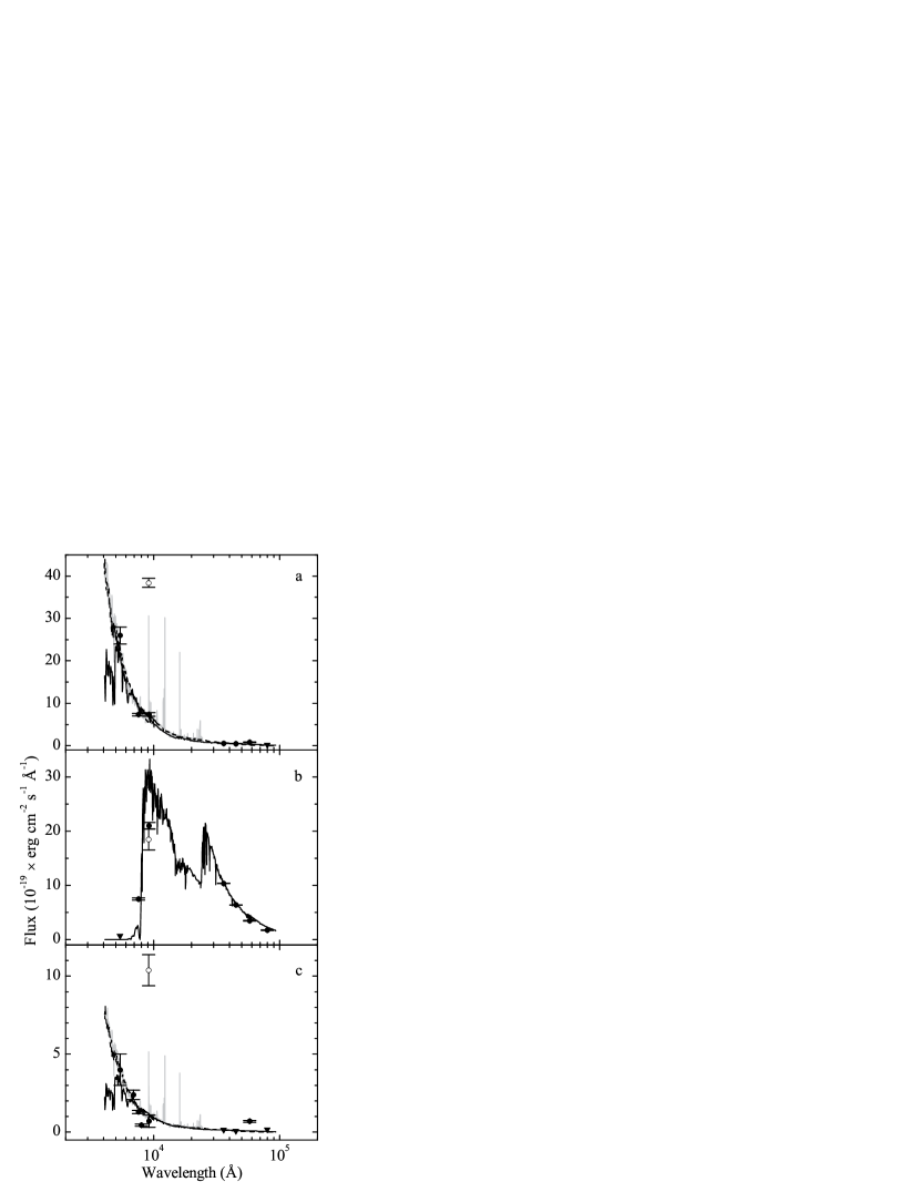
Figure 8: SED fittings for OSIRIS-TF LAE candidates. OSIRIS-TF (hollow circle), Subaru, HST, and Spitzer (filled circles for all three) fluxes are plotted along with SEDs calculated with HyperZ. (a) Candidate $\mathbb{A}$a: the solid line corresponds to the best fit SED, a $z=3.03$ starburst galaxy; the dashed line shows the fit at $z=1.45$ for an [O II] interloper, and the gray line shows a scaled high–resolution version of the previous fit, obtained from a starburst galaxy template by (Calzetti et al., 1994; Kinney et al., 1996). (b) Candidate $\mathbb{A}$b: the best fit corresponds to a $z\simeq 5.4$ LBG. (c) Candidate $\mathbb{A}$c: the best fit is obtained for a $z=3.0$ (solid line) starburst galaxy; dashed and gray lines show the fit and scaled templates for a $z=1.45$ [O II] interloper, as for $\mathbb{A}$a.

$\mathbb{A}$a:

Candidate $\mathbb{A}$a is detected in the Subaru $V$, $i$'  and $z$'  filters; it lies out of the field of the HST images; it is also found in Spitzer images at 3.6–5.8 $\mu\rm{m}$, but not in the 8 $\mu\rm{m}$ band. Figure 8a presents the OSIRIS-TF, Subaru and Spitzer available data for this object, and the SEDs for a starburst galaxy at $z=3.03$ and an [O II] interloper at $z=1.45$. The OSIRIS-TF photometric point shows an excess that may be ascribed to [O II] emission. Figure 8a also shows the optical high resolution SED template for a starburst with E($B-V$)$<$ 0.1 by Calzetti et al. (1994) and Kinney et al. (1996).​. This high resolution template has been moved to the starburst galaxy redshift of $z=1.45$, and it has been scaled using a third-degree polynomial to the low resolution starburst SED template fitted by HyperZ. The resulting optical SED does not pretend to show the actual strengths of the emission lines, but give an idea of what should be their appearance. The $\chi^{2}$, in Table, 3 is not very different for the [O II] emitter and starburst fits. The source is an interloper, and most probably an [O II] emitter.

$\mathbb{A}$b:

Photometric data and SED fitting for candidate $\mathbb{A}$b are shown in Figure 8b. The object is detected in Subaru filters $V$, $i$'  and $z$'; it is is located out of the field of the HST images; it is found in all the Spitzer/IRAC filters.

The photometric profile using only the OSIRIS-TF observations (see Figure 5b), suggests a LAE candidate. The profile of the best starburst SED fit at $z\simeq 5.4$ supports a candidate LBG, in which case the OSIRIS-TF photometry point probably corresponds to a spectral feature in the absorption area around the the 9000 Å wavelength. Therefore, object $\mathbb{A}$b is classified as a possible LBG at $z\gtrsim 5.4$.

Table 3: SED fits

ID	Starburst		[O II]
	Redshift	$\chi^{2}$	$\chi^{2}$
$\mathbb{A}$a	3.0	26.2	31.3
$\mathbb{A}$b	5.4	36.3	$\cdots$
$\mathbb{A}$c	3.0	18.3	19.4
$\mathbb{B}$a	5.4	33.1	$\cdots$
$\mathbb{B}$b	5.3	04.6	05.7
$\mathbb{C}$a	2.4	10.1	$\cdots$
$\mathbb{C}$b	5.5	3.1	$\cdots$

$\mathbb{A}$c:

Figure 8c shows the photometric data for candidate $\mathbb{A}$c, and the SEDs of a starburst galaxy at $z=3.0$ and $z=1.45$. The object appears in all Subaru filters, in the field of the HST program ID5991, and is detected in the Spitzer 5.8 $\mu\rm{m}$ image. Figure 8c is similar to Figure 8a, with the gray line showing the optical high resolution SED template for a starburst with E($B-V$)$<$ 0.1.

The photometric profile of the OSIRIS-TF observations (see Figure 5c) resembles the long wavelength queue of an emission line, but the HST, Subaru and Spitzer data are not consistent with a $z\simeq 6.5$ LAE candidate. The fit for a starburst galaxy at $z=1.45$ matches the OSIRIS-TF photometric point corresponding to the [O II]_{λλ3726,3729} doublet. The $\chi^{2}$ values for the best starburst fit and the [O II] interloper are comparable; altogether the object is likely the later.

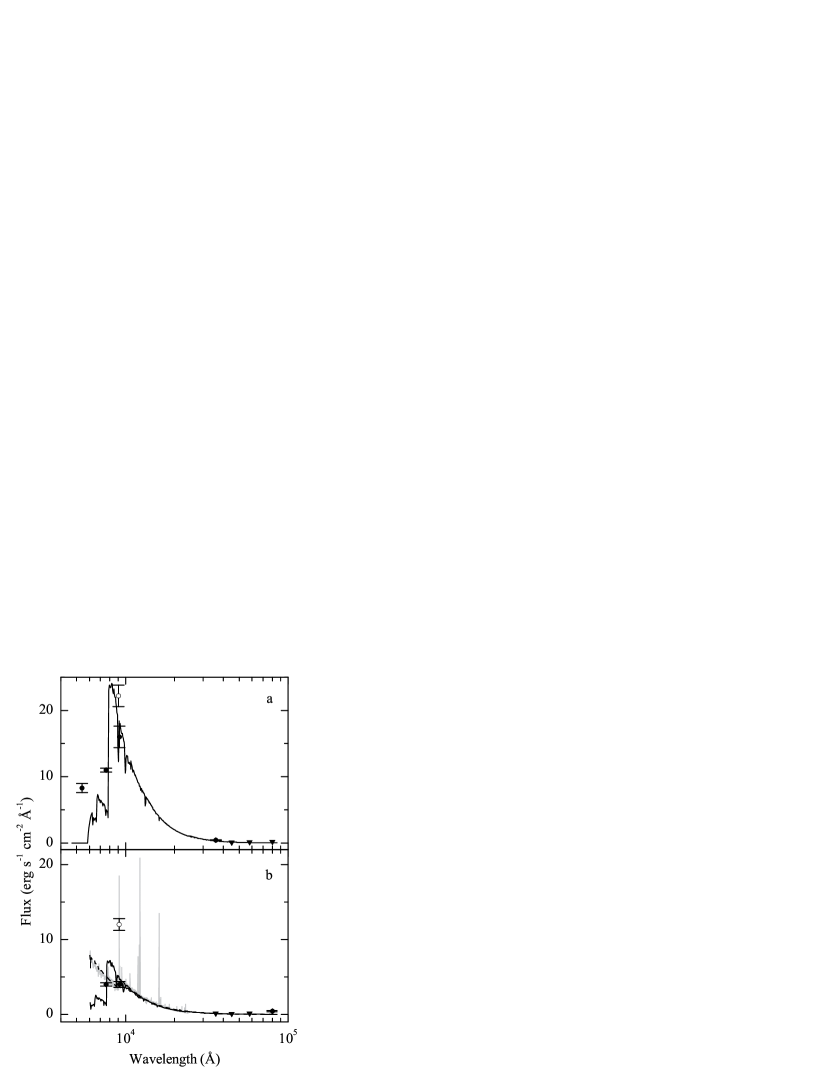
Figure 9: SED fittings for OSIRIS-TF LAE or LBG candidates. Fluxes obtained from OSIRIS-TF (hollow circle) and Subaru, HST, and Spitzer/IRAC (filled circles for the last three) images are plotted, along with SEDs fits calculated with HyperZ. (a) Candidate $\mathbb{B}$a: the SED fit is for a starbusrst galaxy at redshift $z\simeq 5.4$. The object is most likely and interloper. (b) Candidate $\mathbb{B}$b: photometric data have been fitted at $z\simeq 5.3$ (solid line) for a starburst galaxy, and at 1.45 (dashed line) for an [O II] emitter. The best fit suggests a [O II]  interloper at the lowest redshift. The gray line is the same as in $\mathbb{A}$a in Figure 8.

6.4.2 OSIRIS-TF double LAE/LBG candidates

Figure 9 shows the photometry and SED fitting for the OSIRIS-TF double LAE/LBG candidates.

$\mathbb{B}$a:

Candidate $\mathbb{B}$a (shown in Figure 9a) is detected in all of Subaru’s filters; it lies out of the field of the HST images; and it is found in the Spitzer 3.6 $\mu\rm{m}$ band. Figure 9a shows the photometric data available along with the best SED fit for a starburst galaxy at $z\simeq 5.4$. The flux in the OSIRIS-TF synthetic filter may be dominated by the short wavelength queue of an emission line (Figure 6a), which explains that the OSIRIS-TF data is well above the Suprime–Cam $z$'  band. The object is most likely an interloper.

$\mathbb{B}$b:

Figure 9b shows the photometric data for object $\mathbb{B}$b, and the SED of a starburst galaxy at $z\simeq 5.3$ and at $1.45$. The object is detected in the Subaru $i$'  and $z$'  filters; it lies outside of the HST fields; and it is also found in the Spitzer 8 $\mu\rm{m}$ band. Figure 9b is similar to Figure 8a, with the gray line showing the optical high resolution SED template for a starburst with E($B-V$)$<$ 0.1.

Note that, as mentioned earlier, the centroids of the photometrical profiles of the Spitzer/IRAC images for this object are shifted 1$\farcs$3 with respect to their optical counterparts, and thus there is a possibility that the infrared images are misidentified. Both starburst galaxy SED fits are reasonable. However, the OSIRIS-TF flux is well above the Suprime–Cam $z$', suggesting that some of the short wavelength wing of the [O II] line (see Figure 6b) lies in the OSIRIS-TF wavelength range. The object is probably an [O II] interloper.

6.4.3 OSIRIS-TF LBG candidates

Figure 10 shows the photometry and the SEDs of the OSIRIS-TF LBG candidates.

$\mathbb{C}$a:

Images for $\mathbb{C}$a are available through the Subaru $V$ filter, HST program ID6745 and Spitzer 3.6–5.8 $\mu\rm{m}$ bands, remains undetected in the 8 $\mu\rm{m}$ observations and lies outside the field of Subaru’s $i$' and $z$' filters. Figure 10a shows the photometric data for this object (see Figure 7a for the set of OSIRIS-TF observations). The OSIRIS-TF photometric point could correspond with an absorption line. We also plot the best fitting of a SED, that corresponds to a young spiral galaxy at $z\simeq 2.4$. The HST optical data is incongruent with any object at $z>4$. In any case, $\mathbb{C}$a is likely a young spiral galaxy.

$\mathbb{C}$b:

Figure 10b shows the photometric data and the SED of a starburst galaxy at $z=5.5$. The object is detected in Subaru’s $i$'  and $z$'  filters; it lies out of the field of view of the HST images; and it is found in the Spitzer 3.6–5.8 $\mu\rm{m}$ filter but not in the $V$ and 8 $\mu\rm{m}$ bands. The starburst SED fits the photometric data fairly well. The spectral profile observed with OSIRIS-TF (Figure 7b) may in fact be an artefact due to the absorption region at wavelengths longer than the Lyman Break. Nonetheless, the SED fit sustains that $\mathbb{C}$b is a reliable LBG candidate at $z\gtrsim 5.5$ rather than at 6.5 as estimated using only OSIRIS-TF data.

7 Discussion

In this section we compare the results obtained with the different instrumental models applied to our simulated LAE sample, and we examine different explanations for the results of the OSIRIS-TF pilot observations.

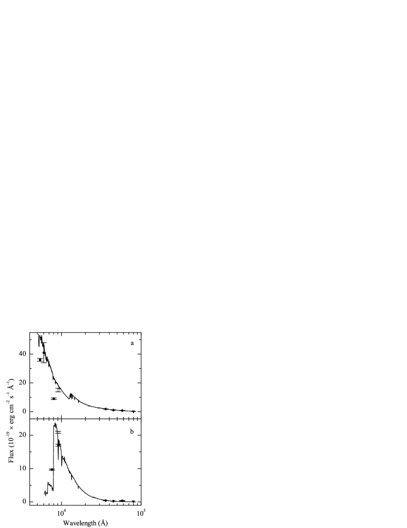
Figure 10: SED fittings for OSIRIS-TF LBG candidates. Fluxes obtained from OSIRIS-TF (hollow circles) and Subaru, HST, and Spitzer/IRAC (filled circles for the last three) images are plotted, along with SEDs calculated with HyperZ. (a) Candidate $\mathbb{C}$a: the best SED fit is that of a spiral galaxy at redshift $z\simeq 2.4$. (b) Candidate $\mathbb{C}$b: the photometric data are consistent with the SED of a starburst galaxy at $z=5.5$; The SED profile suggests the object may be a LBG at $z\gtrsim 5.5$ or a high–redshift interloper.

Table 4: Simulation statistics

Instrument	Parameter	N	Median	Q1	Q3
IDEAL	$z$	1290	6.55	6.53	6.58
	$L_{\rm{Ly\alpha}}$	$\cdots$	6.35	4.16	10.93
	$EW_{0}$	$\cdots$	94	56	175
	$FWHM_{0}$	$\cdots$	1.63	1.25	2.13
Subaru	$z$	1108	6.54	6.51	6.56
	$L_{\rm{Ly\alpha}}$	$\cdots$	7.49	4.85	13.23
	$EW_{0}$	$\cdots$	105	66	187
	$FWHM_{0}$	$\cdots$	1.65	1.26	2.19
OSIRIS-TF	$z$	2708	6.55	6.51	6.59
	$L_{\rm{Ly\alpha}}$	$\cdots$	6.00	3.95	11.14
	$EW_{0}$	$\cdots$	67	34	140
	$FWHM_{0}$	$\cdots$	1.67	1.27	2.16

7.1 Insights from simulated data

Table 4 summarizes the modeled performance for detection of LAEs for the three filter models analyzed in this paper. We present the statistical results using non-parametric scores (sample median and quartiles) since most of the simulated variables are poorly fitted by the Gaussian distribution.

The main differences that can be drawn from Table 4 correspond to the number of detections and the EW distributions of the LAE recovered in each filter. The number of LAEs recovered from our simulation using the NB921 filter in the Subaru Suprime camera and the ideal rectangular filter are similar, but they are only about 40% of those selected using the OSIRIS-TF. These results are explained by the asymmetric continuum bias, the filter profiles, and by the different power of narrow-band and ultra-narrow-band survey methodologies to detect LAEs with small EW values.

It is difficult to detect small EW LAEs. Thus, it is very interesting that the distribution of the equivalent widths at the rest-frame for OSIRIS-TF recovered LAEs shows a median ($\widetilde{EW}_{0}=67$ Å) that is very accurate with respect to the median of the simulations (68 Å), and that is significantly smaller than those of the ideal and NB921 filters (94 and 105 Å, respectively). This result shows that the OSIRIS-TF can extent the search of LAE candidates to objects with a relatively low contrast between the line and the continuum fluxes, which otherwise would be underestimated or even unnoticed in narrow-band surveys. Taking the values of the first quartile for the Subaru’s EW in Table 4, we estimate that many LAEs with $EW(\rm{Ly\alpha})<60$ Å may remain undetected in Subaru’s survey. This would explain the difference between the EW medians for LAEs at redshifts $z\simeq 5.7$ and 6.5 reported by Kashikawa et al. (2011, 89 and 74 Å, respectively), as well as the lack of LAEs between redshifts $6.6<z<7.1$ with $EW(\rm{Ly\alpha})$ in the range between 20 and 55 Å accounted by Pentericci et al. (2011). In fact, these changes in the EW of LAEs are interpreted as a fast evolution of the luminosity of the $\rm{Ly\alpha}$ line caused by the incomplete reionization of the Universe at redshifts $z>6$. If LAEs at $z\simeq 6.5$ and with $EW(\rm{Ly\alpha})<60$ Å were numerous, tunable filter surveys might have a large impact on our knowledge of their LF, changing our current view.

In addition to the EW, the mean luminosity of the $\rm{Ly\alpha}$ line is also 5% and 20% lower for simulated LAEs detected with OSIRIS-TF with respect to those found using the ideal and Subaru filters, respectively. As we mentioned above, the OSIRIS-TF methodology to find LAE candidates presented in this paper is able to find almost all of our simulated objects. Now we see that OSIRIS-TF superior performance respect to the other instruments is not only due to an unbiased wavelength coverage, but also to differences of the line luminosity properties of the detected LAEs.

The distribution of redshifts for the OSIRIS-TF candidates yields the largest interquartile range of $\Delta z=0.08$, in contrast to 0.05 for both the ideal and the NB921 filters. This difference between the OSIRIS-TF and the narrow-band filters is a consequence of the respective filter transmission profiles. On one hand, narrow-band filters tend to be effective in finding LAE candidates on a rather restricted range of wavelengths of the filter bandpass, on the other OSIRIS-TF candidates are evenly distributed on the swept wavelength range between 9122 and 9160 Å. Moreover, the Lorentzian profile of the OSIRIS-TF transmission, extends some filter sensitivity to find LAEs beyond the probed wavelengths. In practice, this will translate in a excess of LAE candidates with upper redshift limits, and an excess of double LAE/LBG candidates with lower redshift limits at the blue and red borders of the set of OSIRIS-TF, respectively, as we have seen with the observed data presented in §5.2. Finally, the distributions of the FWHM at rest-frame do not change significantly among the different filters.

The depth achieved using narrow-band filters in LAE surveys is severely limited by the filter profile. Our results using simulations agree with the analysis of Subaru’s data reported by Kashikawa et al. (2011). Thus, the output varies dramatically along the filter band, reflecting the filter response. In any case, the asymmetric continuum profile at each side of the $\rm{Ly\alpha}$ line introduces a detection bias regardless the profile of the narrow-band filter. This bias is difficult to correct, as it may depend on several factors, such as the actual EW of the $\rm{Ly\alpha}$ line. Therefore, narrow-band surveys are useful to find candidates in a slim volume over a large area, but the properties that can be derived from follow-up spectroscopical observations are prone to produce biased results.

In contrast, the OSIRIS-TF can sample the whole range of the wavelengths of interest with a spectral resolution about 10 times larger than narrow-band filters, and thus the combined $\rm{Ly\alpha}$ line and break features could be recognized, and the redshift determined to a better accuracy (Figure 3). This avoids the biases introduced by the relatively large bandwidth and the extended wings of the transmission profiles of narrow-band filters. LAEs with their $\rm{Ly\alpha}$ line lying between 9122 and 9260 Å are almost completely recovered (Figure 2). However, OSIRIS-TF also has limitations, in particular the amount of total observing time increases with the number of images, which is proportional to the desired spectral resolution. Besides, the OSIRIS-TF relatively small field of view of $8.53\times 8.67\,\rm{arcmin}^{2}$ with a small shadowed area in one side, cannot compare to the wide field of Subaru Suprime-Cam ($34\times 27\,\rm{arcmin}^{2}$). As a low resolution Fabry-Pérot spectrographa, the field of view of tunable filter instruments is limited by the dependence of the effective wavelength on the distance to the optical center (see eq. 5), that would spoil the desired monochromaticity in wide field images (although this effect can be compensated by wavelength scanning at the expense of telescope time). Thus, OSIRIS-TF is an instrument suitable for pencil-beam surveys spanning a relatively large volume, and for assessing the biasses produced by standard narrow-band filter surveys.

We have looked for relationships between the simulated variables. Aside the obvious dependences imposed by candidate selection criteria (e.g. detection and EW limits), there are no practical differences between the detected and non-detected sets of simulated data, regardless of the filter characteristics. The only tiny effects that we have found involves LAES with the largest observed FWHM and located near any of the edges of the filter. Thus, objects near the blue edge, but with the $\rm{Ly\alpha}$ peak off the filter range, may be still detected because part of the flux lies in the filter. On the other hand, objects near the filter red edge may be undetected because the long wavelength queue of the $\rm{Ly\alpha}$ line extends beyond the transmitted wavelengths.

We have also investigated the effect of the number of filters used to detect LAEs. This effect may be present in observational strategies using several narrow bands to detect LAE candidates (or in general any emission objects), such as the OSIRIS-TF procedure discussed in this paper. The particular filter profile may render small changes on the results, and thus we have used ideal filter sets (rather than Gaussian or Lorentzian profiles) to characterize the several sets with different numbers of filters. The filter passband is different for each set, thus they cover the same spectral region and effective volume. In any case, the separation between the centers of two adjacent filter is half of the FWHM of the filter passband, as in the case of the OSIRIS-TF.

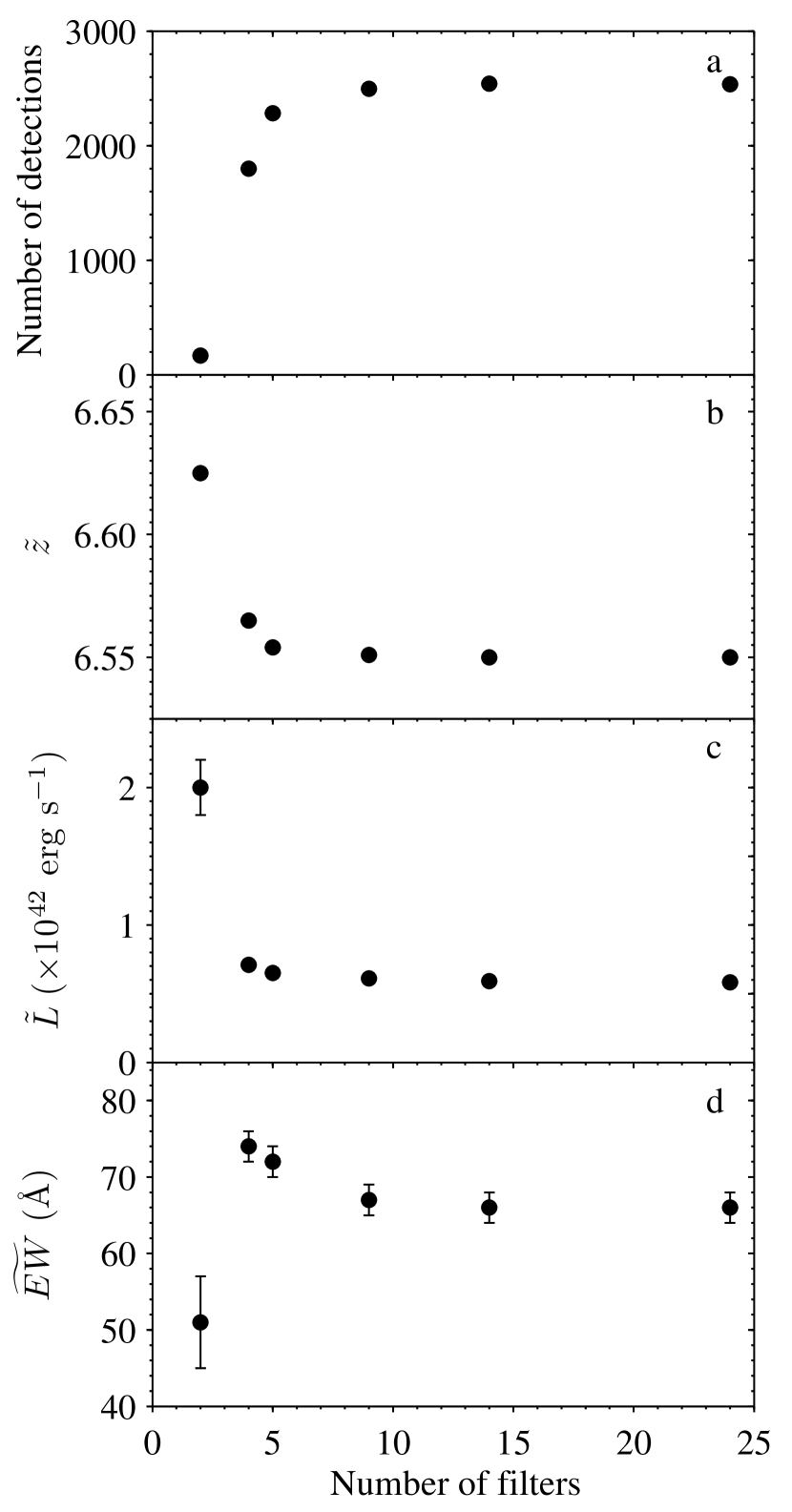
Figure 11: Dependences on the number of filters. This figure shows the results obtained using different sets of ideal (rectangular) filters on the LAE simulation dataset. Each of these sets consist of different number of filters, but they cover the same wavelength range than the original OSIRIS-TF set. Filters in a given set share the same FWHM, and their centers differ in steps of half this FWHM. For detections, we have adopted the same criteria as in the case of OSIRIS-TF. Panels show (a) the number of detections, (b) the median redshift, (c) the line luminosity, and (d) the restframe equivalent width. The results for 7 or more filters are similar, but for smaller number of filters the number of detections falls dramatically, and the other parameters also change significantly.

Table 5: Dependence of detections on the number of filters.

FWHM	Number	Detections	EW0
(Å)	of filters		(Å)
12	24	2535	66$\pm$	2
20	14	2542	66$\pm$	2
30	9	2497	67$\pm$	2
50	5	2282	72$\pm$	2
60	4	1799	74$\pm$	2
100	2	168	51$\pm$	6

Table 5 and Figure 11 summarize the results obtained with different sets of ideal filters. The wavelength range ($r$) at the filters FWHM covered for all the sets is the same, and it is given by the expression:

$$r=\frac{n+1}{2}\,w=150\,\text{\AA},$$ (6)

where $n$ is the number of filters in the set and $w$ is the filter FWHM. We notice that the number of detections, around 2500 objects, decays slightly (3%) from 24 to 9 filters. However, for 5 filters there is a sharp cut-off in this number, and for the set of two filters, only 168 are detected. For the line luminosity and redshift, the change also starts at 5 filters, with increments in their values. The rest-frame EW shows also an increment for 5 filters, but abruptly decays for 2 filter sets. The reason for this decay is that the only 168 objects detected are very luminous in both line and continuum emission. The rest-frame FWHM of the line, not shown in Figure 11, may also show an increment, but it is less significant than for the previous variables. We note that for the 2 filters set the distribution of detected objects becomes bimodal, rather than reflecting the original distribution. This occurs because a line located at the middle of the wavelength range lies in two filters, and our detection algorithm is unable to recognize such a line when the number of filters is small.

For $\rm{Ly\alpha}$ and in general for other single and isolated emission lines, the previous analysis indicates that we might save significant telescope time, and still obtain similar results, observing through 9 filters with FWHM of 30 Å rather than 24 filters with FWHM of 12 Å. In return, the lower spectral resolution may increase the number of interlopers. However, currently the OSIRIS-TF resolution cannot be changed in the wavelength range of our observations. It is worth noting that for other studies where line deblending is necessary, such as mapping H$\alpha$+[N II] or the [S II] doublet, it may be convenient to maintain a filter bandpass lower than 15 Å (e.g. Lara-López et al., 2010; Cedrés et al., 2013).

Table 6: OSIRIS-TF Survey Expected Quantities

	Observations
	Planed	Accomp.
Slices	24	5
Irradiance limit	4	9
LLyα limit	2.1	4.7
Volume LAEs	8760	1503
Expected LAEs	4.2	0.1
L${}_{\mathrm{[O\,{II}]}}$ limit	2.9	6.4
Volume [O II]	122	21
Expected [O II] (Takahashi)	7.4	0.8
Expected [O II] (Dressler)	2.5	0.2

. .

7.2 Excess of candidates and interlopers

The pilot observations obtained with the OSIRIS-TF embrace 5 out of 24 adjacent wavelength slices included in our complete program to find LAE candidates. Table 6 shows the values of some calculated and expected quantities.

Given the LAEs and [O II] interlopers LFs, we hardly expected to find any of these objects in the limited set of observations presented in this paper. Regardless of this prospect, we have extracted five candidates for which OSIRIS-TF data are congruent with LAEs, two of them also LBG candidates (in total, there were four LBG candidates). All of the LAE candidates were rejected after fitting broad-band SEDs, but then three of them showed as possible [O II] interlopers, which is also a number of objects higher than expectations. These discrepancies between the number of expected LAEs and [O II] interlopers, and the actual number of candidates, is explained due to the low number of filters used in our current observations. Thus, the available data expands only a very small range of wavelengths (the FWHM of the synthetic OSIRIS-TF is 36 Å rather than 150 Å for the complete set of 24 filters), preventing a reliable sampling of the line and the continuum to both sides of the line. As a result, we cannot distinguish between small and large FWHM lines because only a part of the wing of a line is observed, or even discriminate between emission lines and partially observed absorption features. These problems can be easily solved by observing through the complete set of filters. Meanwhile, we need to rely on archive data to improve candidate selection. Under these circumstances, even the limited number of broad-band archive data is useful to reject candidates with SED profiles not compatible with LAEs or LBGs, but insufficient to confirm the nature of the objects.

Dressler et al. (2011) have calculated the luminosity function for [O II], [O III], and H$\alpha$ interlopers for LAEs at $z\simeq 5.7$. These LFs have a sharp cut-off for luminosities $\gtrsim 3\times 10^{41}\,\,\rm{erg\,s^{-1}}$, being [O II] emitters the most numerous of the foreground sources. Considering a similar cut-off for $z\simeq 6.5$ interlopers, it corresponds to irradiances $>2.2\times 10^{-17}\,\,\rm{erg\,s^{-1}\,cm^{-2}}$ for [O II]at $z=1.45$, $>9.1\times 10^{-17}\,\,\rm{erg\,s^{-1}\,cm^{-2}}$ for [O III] at $z=0.82$, and $>5.6\times 10^{-17}\,\,\rm{erg\,s^{-1}\,cm^{-2}}$ for H$\alpha$ at $z=0.39$. Our LAE candidates listed in Table 1 have irradiances below all these flux cut-off values, the only exception being $\mathbb{A}$a which slightly exceeds the [O II] flux cut-off. Therefore, interlopers can enhance the number of fake candidates, in accordance with the results obtained when fitting the SEDs in §6.

$\rm{Ly\alpha}$ observed lines at $z=6.5$ are rather wide, with FWHM around 10 Å. Interlopers’ emission lines have observed widths that usually are well below this value. Table 7 shows the observed FWHM for $\rm{Ly\alpha}$ and possible interlopers. For the interlopers, a fiducial velocity for the emission lines arising from Star Formation Regions of 100 $\,\rm{km\,s^{-1}}$ has been chosen. Of course, the interlopers have redshifts $z\ll 6.5$, and thus lower doppler broadening than $\rm{Ly\alpha}$. Then, all the single lines, but the unresolved [O II] blend, have observed FWHM easily distinguishable from the $\rm{Ly\alpha}$ with the OSIRIS spectral resolution. In the case of the [O II] blend, the separation between the individual line peaks, rather than the velocities, dominates the observed FWHM.

Table 7: Observer-frame FWHM for $z\simeq 6.5$ LAEs and interlopers.

Line	Redshift	Velocity	FWHM
		(km s-1)	(Å)
$\rm{Ly\alpha}_{\lambda 1216}$	6.50	400	12.16
[O II]λλ3726-9	1.45	–	$\sim 10\phantom{.00}$
[O III]λ5007	0.82	100	3.04
$\rm{H\alpha_{\lambda 6563}}$	0.39	100	3.04

Given the detection limit for these observations ($9\times 10^{-18}\;\,\rm{erg\,s^{-1}\,cm^{-2}}$), [O II] interlopers at $z\simeq 1.45$ with line luminosities brighter than $L_{\text{[O\,II]}}>1.166\times 10^{41}\;\,\rm{erg\,s^{-1}}$ will be detected. This yields a number of 0.2 – 0.8 expected [O II] interlopers in our data, depending on the luminosity function adopted (Dressler et al., 2011; Takahashi et al., 2007, respectively). Expected numbers for the full set of planed observations are shown in Table 6. From Dressler et al. (2011), we expect a final efficiency of about 2/3 to find LAEs, i.e., 2 LAEs for every [O II] interloper, when the program is fulfilled. The OSIRIS Multi Object Spectrograph-Mode, soon available at the GTC, could be used for follow-ups if necessary.

The lines ratio [O II]$\,\mathrm{\lambda 3726}/$[O II]$\,\mathrm{\lambda 3729}$ between the individual lines that conform the [O II] blend feature depends on the electronic density $N_{\rm{e}}$. Extreme cases have values $\lim_{N_{\rm{e}}\rightarrow 0}=1.5$ and $\lim_{N_{\rm{e}}\rightarrow\infty}=0.35$, and thus this lines ratio can be used to calculate the electronic density when it is in the range $2<\log(N_{\rm{e}})<4$ (Pradhan et al., 2006). Different values of [O II] ratios have a direct incidence on the unresolved blend FWHM measured with OSIRIS-TF, which makes even more difficult to distinguish between LAEs and [O II] interlopers. There are few studies on the LF of [O II], and all of them deal with the blend as a single feature (Hogg et al., 1998; Gallego et al., 2002; Teplitz et al., 2003; Takahashi et al., 2007; Dressler et al., 2011).

An effect to take into account is the distortion of the observed LAEs and [O II] interlopers LF, and thus their number counts, due to the redshift dependent magnification bias (e.g. Bartelmann, 2010; de Diego et al., 2011). This effect increases the number of observed faint sources, but reduces their number density enlarging the angular distance between the sources. The overall result depends on the steepness of the number-count function. For the high luminosity LAEs, such as those observed at $z\sim 6.5$, this function is steep and more sources become observable. The situation is more complex for [O II] interlopers, for which the high luminosity objects do not dominate the number counts. Thus, the magnification bias may reduce the number of observed [O II] interlopers with luminosities below $\simeq 3\times 10^{41}\,\,\rm{erg\,s^{-1}}$, and enhances the counts for more luminous sources. In our case, the field observed with the OSIRIS-TF is dominated by the cluster of galaxies MS 2053.7-0449 at redshift $z=0.583$, that expands about $4\times 7\,\rm{arcmin}^{2}$. The cluster contains a gravitational lensed arc (Luppino & Gioia, 1992; Tran et al., 2005). The strong gravitational lens model has been discussed by Verdugo et al. (2007), and the weak-lensing signature of the cluster was detected by Hoekstra et al. (2002), who estimated a cluster velocity dispersion of $886\,\rm{km\,s^{-1}}$.

Following Hildebrandt et al. (2011), we have used the singular isothermal sphere approximation to calculate the lens magnification as a function of the angular separation $\theta$ from the cluster center:

$$\mu(\theta)=\frac{\theta}{\theta-\theta_{E}},$$ (7)

where $\theta_{E}$ is the Einstein radius (Narayan & Bartelmann, 1996) for the cluster:

$$\theta_{E}=4\pi\left(\frac{\sigma_{v}}{c}\right)^{2}\frac{D_{ds}}{D_{s}},$$ (8)

and where $\sigma_{v}$ is the one-dimensional velocity dispersion (we have adopted Hoekstra et al., 2002, estimate of $886\,\rm{km\,s^{-1}}$), $D_{ds}$ is the angular diameter distance from the lensing cluster to the source, and $D_{s}$ is the angular diameter distance from the observer to the source. We have taken a common redshift of $z=6.5$ for LAEs and $z=1.45$ for [O II] interlopers. In our case, the Einstein radius for MS 2053.7-0449 is $\theta_{E}=17\arcsec$ and $11\arcsec$ for LAEs and [O II] interlopers, respectively.

The mean magnification $\left<\mu\right>_{wl}$ in the weak lensing regime of the OSIRIS-TF field around MS 2053.7-0449 can be calculated considering an angular separation $3\theta_{E}\leq\theta\leq 4\arcmin$ which ranges from the weak lensing limit to the edge of the detector:

$$\left<\mu\right>_{wl}=\frac{\int^{4\arcmin}_{3\theta_{E}}\mu(\theta)\;\rm{d}\theta}{\int^{4\arcmin}_{3\theta_{E}}\rm{d}\theta},$$ (9)

yielding mean magnifications of 1.17 for LAEs and 1.13 for [O II] interlopers. Figure 12 shows the change of the magnification with the distance to the cluster center. For the planed sample, this magnification yields an increase from 4.2 to 5.7 for expected LAE counts. However, for the currently observed bands, the expected number of LAEs has a negligible increase of about 0.1 objects. As discussed above, the case of [O II] interlopers is more complicated, and depends on the actual profile of their LF.

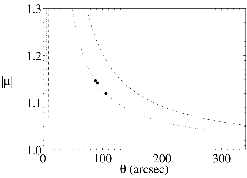
Figure 12: Magnification as a function of the angular separation to the center of the cluster of galaxies. The dotted line shows the absolute value of the magnification $\mu$ as a function of the angular separation $\theta$ for the cluster MS 2053.7-0449, using a singular isothermal sphere model. Filled circles correspond to [O II] interloper candidates.

A major concern with photometric searches of LAE candidates is that only a tight range of redshifts is probed, yielding small samples prone to cosmic variance due to large-scale density fluctuations. Cosmic variance accounts for deviations from the factual or expected values of the number-counts of rare phenomena, and of objects found in small volume surveys. Following Trenti & Stiavelli (2008), we have calculated that the uncertainty on the number-counts is $\sigma_{counts}=1$ for both LAEs and [O II] interlopers. Moreover, [O II] emitters are likely to show strong cross-correlation positions (Dressler et al., 2011). Therefore, we do not discard the possibility that some interloper candidates are actually [O II] emitters.

8 Conclusions

Narrow-band surveys allow to sample large sky areas and have been successful in finding LAE candidates. However, we have shown that the asymmetrical profile of the continuum around the $\rm{Ly\alpha}$ line in LAEs yields a detection bias that affects the performance to find objects at redshifts where the $\rm{Ly\alpha}$ line lies near the long wavelength edge of narrow-band photometric filters. Therefore, the Subaru survey and others that might be conducted using narrow-band filters, are prone to yield a biased LF. Besides, this methodology tends to ignore or underestimate small EW objects.

In the case of ultra-narrow-band surveys, our simulations show that the overall performance for LAE detection using OSIRIS-TF is not affected by the filter transmission profile, and the LF of LAEs could be accurately calculated. Moreover, OSIRIS-TF can recover simulated LAEs with $\rm{Ly\alpha}$ line EWs significantly smaller than the objects recovered with narrow-band filters. Nonetheless, tunable filters do not produce large monochromatic images, and the number of ultra-narrow-band images increases in proportion to the required spectral resolution, thus the size of the studied area is limited for practical reasons. Therefore, both narrow-band and ultra-narrow-band surveys have different strengths and weaknesses, and thus they must be regarded as complementary strategies to study high-redshift LAEs.

We are carrying on a program to find LAE candidates with the OSIRIS-TF at the GTC. Part of this program is devoted to find candidates at redshift $z\simeq 6.5$, with an strategy based on our study with Monte Carlo data. We have already performed pilot observations of five sets of images with the GTC and the OSIRIS-TF instrument at adjacent wavelengths, which is a fraction of the 24 wavelength slices that we plan to observe. The OSIRIS-TF images are separated by wavelength steps of 6 Å, and have a bandpass of 12 Å, covering a wavelength range of about 36 Å. The total exposure time in each wavelength is 630 s, rendering a detection level of $9\times 10^{-18}\,\,\rm{erg\,s^{-1}\,cm^{-2}}$, which is about two times less sensitive than that reported for the Subaru LAE surveys. Available Subaru, HST/WFPC2 and Spitzer/IRAC archive data have been employed to build SED models. Because of the limited wavelength range of OSIRIS-TF observations, these models have been very helpful to reject LAE and LBG candidates and to identify interlopers, although the low number of bands used in the fits prevents accurate object classification and redshift estimate.

We have calculated the number of expected LAEs in the OSIRIS-TF field with our observational conditions. For this purpose, we have taken into account the weak lensing effect introduced by a nearby cluster of galaxies, and the effect of the cosmic variance. Thus, we expected no more than one possible LAE and [O II] interloper showing up in our data. Actually, we have identified three possibly [O II] interlopers, and one LBG candidate. The possible overabundance of [O II] interlopers in the field might be a result of cross-correlation positions (Dressler et al., 2011). In any case, these results support the capabilities of OSIRIS-TF to perform an accurate survey of emission-line objects.

Future work

We plan to complete the set of OSIRIS-TF 24 wavelength slices to extract a sample of high-redshift candidates, namely LAEs, LBGs and high-redshift interlopers. The sample will be studied to confirm the nature of the objects using OSIRIS Multi-Object Spectrograph when available.

References

- Atek et al. (2008) Atek, H., Kunth, D., Hayes, M., Östlin, G., & Mas-Hesse, J. M. 2008, A&A, 488, 491
- Atek et al. (2009) Atek, H., Kunth, D., Schaerer, D., et al. 2009, A&A, 506, L1
- Bartelmann (2010) Bartelmann, M. 2010, Gravitational Lensing, arXiv:1010.3829
- Bertin & Arnouts (1996) Bertin, E., & Arnouts, S. 1996, A&AS, 117, 393
- Blanc et al. (2011) Blanc, G. A., Adams, J. J., Gebhardt, K., et al. 2011, ApJ, 736, 31
- Blanton & Lin (2000) Blanton, M., & Lin, H. 2000, ApJ, 543, L125
- Bolzonella et al. (2000) Bolzonella, M., Miralles, J.-M., & Pelló, R. 2000, A&A, 363, 476
- Bruzual & Charlot (2003) Bruzual, G., & Charlot, S. 2003, MNRAS, 344, 1000
- Bruzual A. & Charlot (1993) Bruzual A., G., & Charlot, S. 1993, ApJ, 405, 538
- Calzetti et al. (1994) Calzetti, D., Kinney, A. L., & Storchi-Bergmann, T. 1994, ApJ, 429, 582
- Cedrés et al. (2013) Cedrés, B., Beckman, J. E., Bongiovanni, Á., et al. 2013, ApJ, 765, L24
- Cepa (2009) Cepa, J. 2009, TF User Manual, Tech. rep., Instituto de Astrofísica de Canarias
- Cepa et al. (2003) Cepa, J., Aguiar, M., Bland-Hawthorn, J., et al. 2003, RMxAACS, 16, 13
- Cepa et al. (2011) Cepa, J., Alfaro, E., Bongiovanni, A., et al. 2011, OSIRIS: User Manual (Scientific Use), Tech. rep., Instituto de Astrofísica de Canarias
- Ciardullo et al. (2012) Ciardullo, R., Gronwall, C., Wolf, C., et al. 2012, ApJ, 744, 110
- Cowie & Hu (1998) Cowie, L. L., & Hu, E. M. 1998, AJ, 115, 1319
- Dayal & Ferrara (2012) Dayal, P., & Ferrara, A. 2012, MNRAS, 2461
- de Diego et al. (2011) de Diego, J. A., Cepa, J., De Leo, M., & Bongiovanni, Á. 2011, Journal of Physics: Conference Series, 314, 012119
- Dijkstra et al. (2007) Dijkstra, M., Lidz, A., & Wyithe, J. S. B. 2007, MNRAS, 377, 1175
- Dressler et al. (2011) Dressler, A., Martin, C. L., Henry, A., Sawicki, M., & McCarthy, P. 2011, ApJ, 740, 71
- Finkelstein et al. (2011) Finkelstein, S. L., Cohen, S. H., Moustakas, J., et al. 2011, ApJ, 733, 117
- Finkelstein et al. (2008) Finkelstein, S. L., Rhoads, J. E., Malhotra, S., Grogin, N., & Wang, J. 2008, ApJ, 678, 655
- Forero-Romero et al. (2012) Forero-Romero, J. E., Yepes, G., Gottlöber, S., & Prada, F. 2012, MNRAS, 419, 952
- Gallego et al. (2002) Gallego, J., García-Dabó, C. E., Zamorano, J., Aragón-Salamanca, A., & Rego, M. 2002, ApJ, 570, L1
- González et al. (2013) González, J. J., Cepa, J., González-Serrano, I., et al. 2013, OSIRIS/GTC Red Tunable Filter: Wavelength variations across the Field of view. The anomalous phase effect, in preparation
- Gronwall et al. (2007) Gronwall, C., Ciardullo, R., Hickey, T., et al. 2007, ApJ, 667, 79
- Hansen & Oh (2006) Hansen, M., & Oh, S. P. 2006, MNRAS, 367, 979
- Hatziminaoglou et al. (2000) Hatziminaoglou, E., Mathez, G., & Pelló, R. 2000, A&A, 359, 9
- Hayes & Östlin (2006) Hayes, M., & Östlin, G. 2006, A&A, 460, 681
- Hayes et al. (2010) Hayes, M., Östlin, G., Schaerer, D., et al. 2010, Natur, 464, 562
- Hibon et al. (2012) Hibon, P., Kashikawa, N., Willott, C., Iye, M., & Shibuya, T. 2012, ApJ, 744, 89
- Hildebrandt et al. (2011) Hildebrandt, H., Muzzin, A., Erben, T., et al. 2011, ApJ, 733, L30
- Hoekstra et al. (2002) Hoekstra, H., Franx, M., Kuijken, K., & van Dokkum, P. G. 2002, MNRAS, 333, 911
- Hogg et al. (1998) Hogg, D. W., Cohen, J. G., Blandford, R., & Pahre, M. A. 1998, ApJ, 504, 622
- Hu & Cowie (2006) Hu, E. M., & Cowie, L. L. 2006, Natur, 440, 1145
- Hu et al. (2004) Hu, E. M., Cowie, L. L., Capak, P., et al. 2004, AJ, 127, 563
- Kashikawa et al. (2007) Kashikawa, N., Kitayama, T., Doi, M., et al. 2007, ApJ, 663, 765
- Kashikawa et al. (2006) Kashikawa, N., Shimasaku, K., Malkan, M. A., et al. 2006, ApJ, 648, 7
- Kashikawa et al. (2011) Kashikawa, N., Shimasaku, K., Matsuda, Y., et al. 2011, ApJ, 734, 119
- Kinney et al. (1996) Kinney, A. L., Calzetti, D., Bohlin, R. C., et al. 1996, ApJ, 467, 38
- Krug et al. (2012) Krug, H. B., Veilleux, S., Tilvi, V., et al. 2012, ApJ, 745, 122
- Kunth et al. (1998) Kunth, D., Mas Hesse, J. M., Terlevich, E., et al. 1998, A&A, 334, 11
- Lara-López et al. (2010) Lara-López, M. A., Cepa, J., Castañeda, H., et al. 2010, PASP, 122, 1495
- Luppino & Gioia (1992) Luppino, G. A., & Gioia, I. M. 1992, A&A, 265, L9
- Malhotra & Rhoads (2004) Malhotra, S., & Rhoads, J. E. 2004, ApJ, 617, L5
- Mallery et al. (2012) Mallery, R. P., Mobasher, B., Capak, P., et al. 2012, ApJ, 760, 128
- Narayan & Bartelmann (1996) Narayan, R., & Bartelmann, M. 1996, Lectures on Gravitational Lensing, arXiv:astro-ph/9606001
- Neufeld (1991) Neufeld, D. A. 1991, ApJ, 370, L85
- Ono et al. (2010) Ono, Y., Ouchi, M., Shimasaku, K., et al. 2010, ApJ, 724, 1524
- Ono et al. (2012) Ono, Y., Ouchi, M., Mobasher, B., et al. 2012, ApJ, 744, 83
- Ota & Iye (2012) Ota, K., & Iye, M. 2012, MNRAS, 423, 444
- Ota et al. (2010) Ota, K., Iye, M., Kashikawa, N., et al. 2010, ApJ, 722, 803
- Ouchi et al. (2008) Ouchi, M., Shimasaku, K., Akiyama, M., et al. 2008, ApJS, 176, 301
- Ouchi et al. (2010) Ouchi, M., Shimasaku, K., Furusawa, H., et al. 2010, ApJ, 723, 869
- Pentericci et al. (2011) Pentericci, L., Fontana, A., Vanzella, E., et al. 2011, ApJ, 743, 132
- Pradhan et al. (2006) Pradhan, A. K., Montenegro, M., Nahar, S. N., & Eissner, W. 2006, MNRAS, 366, L6
- Santos et al. (2004) Santos, M. R., Ellis, R. S., Kneib, J.-P., Richard, J., & Kuijken, K. 2004, ApJ, 606, 683
- Schenker et al. (2012) Schenker, M. A., Stark, D. P., Ellis, R. S., et al. 2012, ApJ, 744, 179
- Shapley et al. (2001) Shapley, A. E., Steidel, C. C., Adelberger, K. L., et al. 2001, ApJ, 562, 95
- Shapley et al. (2003) Shapley, A. E., Steidel, C. C., Pettini, M., & Adelberger, K. L. 2003, ApJ, 588, 65
- Shibuya et al. (2012) Shibuya, T., Kashikawa, N., Ota, K., et al. 2012, ApJ, 752, 114
- Shimasaku et al. (2006) Shimasaku, K., Kashikawa, N., Doi, M., et al. 2006, PASJ, 58, 313
- Stark et al. (2010) Stark, D. P., Ellis, R. S., Chiu, K., Ouchi, M., & Bunker, A. 2010, MNRAS, 408, 1628
- Stark et al. (2011) Stark, D. P., Ellis, R. S., & Ouchi, M. 2011, ApJ, 728, L2
- Steidel et al. (1996) Steidel, C. C., Giavalisco, M., Pettini, M., Dickinson, M., & Adelberger, K. L. 1996, ApJ, 462, L17
- Swinbank et al. (2012) Swinbank, J., Baker, J., Barr, J., Hook, I., & Bland-Hawthorn, J. 2012, MNRAS, 422, 2980
- Takahashi et al. (2007) Takahashi, M. I., Shioya, Y., Taniguchi, Y., et al. 2007, ApJS, 172, 456
- Taniguchi et al. (2005) Taniguchi, Y., Ajiki, M., Nagao, T., et al. 2005, PASJ, 57, 165
- Tapken et al. (2007) Tapken, C., Appenzeller, I., Noll, S., et al. 2007, A&A, 467, 63
- Teplitz et al. (2003) Teplitz, H. I., Collins, N. R., Gardner, J. P., Hill, R. S., & Rhodes, J. 2003, ApJ, 589, 704
- Tilvi et al. (2010) Tilvi, V., Rhoads, J. E., Hibon, P., et al. 2010, ApJ, 721, 1853
- Tran et al. (2005) Tran, K.-V. H., van Dokkum, P., Illingworth, G. D., et al. 2005, ApJ, 619, 134
- Trenti & Stiavelli (2008) Trenti, M., & Stiavelli, M. 2008, ApJ, 676, 767
- Vanzella et al. (2011) Vanzella, E., Pentericci, L., Fontana, A., et al. 2011, ApJ, 730, L35
- Verdugo et al. (2007) Verdugo, T., de Diego, J. A., & Limousin, M. 2007, ApJ, 664, 702
- Verhamme et al. (2008) Verhamme, A., Schaerer, D., Atek, H., & Tapken, C. 2008, A&A, 491, 89
- Verhamme et al. (2006) Verhamme, A., Schaerer, D., & Maselli, A. 2006, A&A, 460, 397