Abstract

We study a lattice sigma model which is expected to reflect Anderson localization and delocalization transition for real symmetric band matrices in 3D, but describes the mixing measure for a vertex reinforced jump process too. For this model we prove exponential localization at any temperature in a strip, and more generally in any quasi-one dimensional graph, with pinning (mass) at only one site. The proof uses a Mermin-Wagner type argument and a transfer operator approach.

1 Introduction

Nonlinear sigma models and random matrices.

Nonlinear sigma models appear as effective models at low energy in a large variety of physical problems where some kind of spontaneous symmetry breaking and phase transition is expected. They can be viewed, in analogy to statistical mechanics, as models of interacting spins, taking values in a nonlinear manifold. In the context of disordered conductors and quantum chaos, the spectral and transport properties of random Schrödinger operators and random band matrices can be translated in the study of the correlation functions for a statistical mechanics model where the spin at each lattice site $j$ is replaced by a matrix $Q_{j}$, whose elements are both ordinary (bosonic) complex or real variables and anticommuting (fermionic) Grassmann variables. This representation was introduced and developed by Efetov [Efe83, Efe97], based on seminal work by Wegner [Weg79, SW80], using the supersymmetric approach. In the corresponding nonlinear sigma model, the matrix $Q_{j}$ satisfies $Q_{j}^{2}=\mathbf{1}$ and is restricted to take values on a supermanifold, whose symmetry properties depend on the symmetries of the initial random matrix ensemble and the observable (correlation function) under study. Efetov’s supersymmetric nonlinear sigma model and its variants were intensively studied, especially in the physics literature, but they still defy a rigorous mathematical understanding. See [Spe12, Mir00b, Mir00a, Fyo02] for an introduction to these problems.

In this context Zirnbauer introduced a supersymmetric sigma model [Zir91, DFZ92], that is expected to reflect Anderson localization and delocalization transition for real symmetric band matrices in 3D. In this statistical mechanical model the field (or spin) at site $j$ is a vector $v_{j}=(x_{j},y_{j},z_{j},\xi_{j},\eta_{j})$ where $x,y,z$ are real and $\xi,\eta$ are Grassmann variables. We endow this vector space with a generalization of the Lorentz metric $(v,v^{\prime})=xx^{\prime}+yy^{\prime}-zz^{\prime}+\xi\eta^{\prime}-\eta\xi^{\prime}$. Imposing the constraint $(v_{j},v_{j})=-1$, the field $v_{j}$ has four degrees of freedom (two bosonic and two fermionic), and takes values in a target space denoted by $H^{2|2}$, which is a supermanifold extension of the hyperbolic plane $H^{2}$. The effective action for this model is given by

$$\mathcal{F}(v)=\sum_{i\sim j}\frac{\beta_{ij}}{2}(v_{i}-v_{j},\,v_{i}-v_{j})+\sum_{j}\varepsilon_{j}(z_{j}-1)$$ (1.1)

where the first term is the kinetic energy, and $i\sim j$ denotes edges connecting nearest neighbors $i$ and $j$. See [DSZ10, Sect. 2.1] for more details. The parameter $\beta_{ij}=\beta_{ji}>0$ may be seen as a local inverse temperature along the edge $i\sim j$, using the language of statistical mechanics. The last term in the action is needed to break the non-compact symmetry and make the corresponding integral finite, so $\varepsilon_{j}\geq 0$ can be seen as the analog of a magnetic field, or a mass term. Note that if we add a new vertex $\rho$ to the lattice, we connect it to all lattice points $j$ with $\varepsilon_{j}>0$ and we fix $v_{\rho}=(0,0,1,0,0)$ we have

$$\sum_{j}\varepsilon_{j}(z_{j}-1)=\sum_{j}\frac{\varepsilon_{j}}{2}(v_{j}-v_{\rho},v_{j}-v_{\rho}).$$

Then the mass term may be seen as a kinetic term too. In the appropriate coordinate system (see [DSZ10]) the action becomes quadratic in the fermionic variables and these variables can be integrated out exactly. We are left with two real variables $t_{j},s_{j}$ at each lattice site and a probability measure $d\mu(t,s)$. The resulting statistical mechanical model then has a probabilistic interpretation. In this paper, we will not use the supersymmetric formalism at all, and will work directly on the probability measure $d\mu(t,s)$, whose precise form is given in (2.3) below.

Connection with stochastic processes.

Recently Sabot and Tarrès [ST12] proved a precise relation between $H^{2|2}$ and both vertex reinforced jump process (VRJP) and linearly edge reinforced random walk (LERRW) on the graph with the additional vertex $\rho$. Both are history dependent stochastic processes, describing self-organization and learning behavior. VRJP was conceived by Werner and studied in [DV02, DV04, Col06, Col09, BS12]. It is a continuous time process $Y=(Y_{u})_{u\geq 0}$ where the particle jumps from the lattice site $i$ to $j$ with rate $\beta_{ij}(1+L_{j}(u))$, where $L_{j}(u)$ is the local time at $j$, that is the time the particle has already spent on $j$ up to time $u$. Here we take the convention $\beta_{i\rho}=\beta_{\rho i}=\varepsilon_{i}$. In this context large/small $\beta$ corresponds to weak/strong reinforcement. Indeed, assuming $\beta$ to be constant, we can rescale the time by $u^{\prime}=\beta u$. Then $L^{\prime}_{j}(u^{\prime})=\beta L_{j}(u)$, the jump rate becomes $1+L^{\prime}_{j}(u^{\prime})/\beta$ and the bigger $\beta$ is, the weaker the influence of the local time. Let $\tilde{Y}=(\tilde{Y}_{n})_{n\in\mathbb{N}_{0}}$ be the discrete time process associated to $Y$ by taking only the value of $Y_{u}$ immediately before the jump times, ignoring the waiting time between jumps. Sabot-Tarrès [ST12] proved that on any finite graph it can be represented as a random walk in a random environment, and more precisely as a mixture of reversible Markov chains

$$\mathbb{P}(\tilde{Y}\in A)=\int\mathbb{P}^{W(t,s)}(\tilde{Y}\in A)\ d\mu(t,s)$$ (1.2)

for any event $A$ on paths, where $d\mu(t,s)$ is the measure for $H^{2|2}$ defined in (2.3) below. Here $\mathbb{P}^{W(t,s)}(\tilde{Y}\in\cdot)$ is the probability law associated to the Markovian random walk starting at the root $\rho$ and jumping from $i$ to $j$ with probability proportional to $W_{ij}(t,s)=W_{ji}(t,s)=\beta_{ij}e^{t_{i}+t_{j}}$ for any $i\sim j$, with the convention $t_{\rho}=0$. The probability measure $\mu(W\in\cdot)$ allows to pick randomly the environment where the particle moves. It is called the mixing measure for the process. From the stochastic process perspective, the most natural situation is to consider the case of one pinning point $\varepsilon_{j}=\varepsilon\delta_{jj_{0}}$, where $j_{0}$ is some fixed lattice site.

LERRW is a discrete time process $X=(X_{n})_{n\in\mathbb{N}_{0}}$ where the particle jumps at time $n$ from the lattice site $i$ to $j$ with a probability depending on the number of times it has traversed the $i\sim j$ edge in the past. This model is known to be a mixture of reversible Markov chains with explicitly known mixing measure [CD86, KR00]. The relation of this model to $H^{2|2}$ was clarified by Sabot and Tarrès [ST12, Thm. 1], who showed that LERRW is obtained from the discrete time VRJP as a mixture by taking the weights $(\beta_{ij})$ in $W_{ij}(t,s)$ to be independent Gamma distributed random variables. Using this relation they proved localization of LERRW in $d\geq 1$ for strong reinforcement.

Results and conjectures.

Exponential localization for $H^{2|2}$ was established in $d=1$ [Zir91]-[DS10] for any value of $\beta$, and in $d\geq 1$ for small $\beta$ [DS10]. A quasi-diffusive phase was established in $d\geq 3$ for large $\beta$ thus proving the existence of a phase transition [DSZ10]. In $d=2$ localization is expected to hold for any value of $\beta$, with localization length of order $e^{\beta}$. The proofs in [DS10, DSZ10] are derived for constant parameters $\beta_{ij}=\beta$, but they can be easily generalized to the case of variable betas. In the case of one pinning point $\varepsilon_{j}=\delta_{jj_{0}}$, the results listed above imply that the corresponding VRJP starting at $j_{0}$ is recurrent in $d=1$ for any value of $\beta$, and in $d\geq 1$ for small $\beta$ [ST12].

In this paper we consider $H^{2|2}$ in the case of one pinning point on a generalized strip, consisting of copies of an arbitrary finite connected graph. For this model we prove exponential localization for any periodic choice of $\beta_{ij}$, uniformly in the number of copies. This implies the corresponding discrete time process associated to VRJP is recurrent on the infinite strip and exponentially localized in a finite region with high probability: $\mathbb{P}(|\tilde{Y}_{n}|>R)\leq e^{-cR}$ for some constant $c$, independent from $n$. Similar statements could be made about the continuous time process too, although they are not worked out here.

Idea of the proof.

Though one may expect this should be just a small modification of the $1D$ proof, it turns out the argument used in [DS10] breaks down as soon as we leave the perfect one dimensional chain, unless we take $\beta$ small. Here we use a quite different approach, namely a deformation argument on probability measures (in the spirit of Mermin-Wagner). The transfer operator method is used in a non standard way. Instead of estimating the top eigenvalue directly, it is used to bound some of the terms generated by the deformation uniformly in the length of the strip. For this purpose, we need only a reflection symmetry and compactness. To set up a transfer operator we need to express our measure as a product of local functionals. This is not trivial due to the presence of a highly non local determinant in the measure. One might write this determinant in terms of a product of local functions of Grassmann (anticommuting) variables, but would have to deal with a transfer matrix involving both real and Grassmann variables. In contrast, here we write the determinant as a sum over spanning trees, using the matrix-tree theorem. Then these trees can be described by a set of local variables and the Boltzmann weight becomes a product of local non-negative functions.

The arguments are inspired by the methods used by two of us in previous work on the LERRW [MR05, MR09a]. In contrast to that work though, here our deformation depends on a cut-off function selecting only small gradients. With this choice, we have to estimate bounded observables only. An alternative method, not presented here, would be to remove the cut-off function, and deal with unbounded observables.

To simplify the proof as much as possible, we did not try to estimate the localization length as a function of $\beta$ or $W$, though such an estimate is maybe achievable by a more detailed analysis. Some variant of the arguments we use here may perhaps be applied to the case of uniform pinning $\varepsilon_{j}=\varepsilon$. On the other hand, the true $d=2$ case with large beta is much harder and will probably need a different approach.

Acknowledgements. It is our pleasure to thank T. Spencer for many useful discussions and suggestions related to this paper.

2 Model and main result

2.1 The model

Let $G_{0}=(V_{0},E_{0})$ be a finite undirected graph with vertex set $V_{0}$ and edge set $E_{0}$. If there is an edge between $v$ and $v^{\prime}$ in the graph $G_{0}$, we write $(v\sim v^{\prime})\in E_{0}$. We consider the sigma model on the graph ${\mathcal{G}}$ obtained by putting infinitely many copies of $G_{0}$ in a row. Let $G_{n}=(V_{n},E_{n})$ be the copy of $G_{0}$ at level $n\in{\mathbb{Z}}$. More precisely, ${\mathcal{G}}=(V,E)$ has vertex set $V:={\mathbb{Z}}\times V_{0}$ and edge set $E=\bigcup_{n\in\mathbb{Z}}(E_{n}\cup E_{n+1/2})$, where

$$E_{n}:=\{e_{n}:=((n,v)\sim(n,v^{\prime})):\;e=(v\sim v^{\prime})\in E_{0}\}$$ (2.1)

is the set of “vertical” edges in $G_{n}$, connecting the copies at level $n$ of the vertices $v$ and $v^{\prime}$, for any edge $(v\sim v^{\prime})\in E_{0}$, and

$$E_{n+1/2}:=\{v_{n+1/2}:=((n,v)\sim(n+1,v)):\;v\in V_{0}\}$$ (2.2)

is the set of “horizontal” edges connecting each vertex in $V_{n}$ with its copy in $V_{n+1}$. We say that an edge in $E_{n+1/2}$ is at level $n+1/2$. Note that, in the special case when $G_{0}$ is a finite segment of $\mathbb{Z}$, the graph we obtain is an infinite strip. In this case the edges $e_{n}$ are vertical lines while the edges $v_{n+1/2}$ are horizontal lines. Hence, the names above.

For ${\underline{L}},{\overline{L}}\in{\mathbb{N}}$, we set $L:=(-{\underline{L}},{\overline{L}})$ and consider the finite piece ${\mathcal{G}}_{L}=(V_{L},E_{L})$ of ${\mathcal{G}}$ with vertex set $V_{L}:=\{-{\underline{L}},\ldots,{\overline{L}}\}\times V_{0}$. Let $p$ be a fixed vertex in $V_{0}$. We abbreviate ${\mathbf{0}}:=(0,p)$. The site ${\mathbf{0}}$ in $G_{0}$ will be used as pinning point (hence the name we chose). To each site $j\in V_{L}$ we associate the real variables $t_{j}$ and $s_{j}$. We abbreviate $t=(t_{i})_{i\in V_{L}}$ and $s=(s_{i})_{i\in V_{L}}$ and let $\nabla t=(t_{i}-t_{j})_{i,j\in V_{L}}$ denote the vector of gradients of the $t$ variables. We introduce the probability measure

$$d\mu^{{\mathbf{0}}}_{L}(t,s)=\prod_{j\in V_{L}}\frac{dt_{j}ds_{j}e^{-t_{j}}}{2\pi}e^{-F_{L}(\nabla t)}e^{-\frac{1}{2}[s,A_{L}(t)s]}\det[A_{L}(t)+\widehat{\varepsilon}\,]\,e^{-M(t_{{\mathbf{0}}},s_{{\mathbf{0}}})},$$ (2.3)

where $dt_{j}$ and $ds_{j}$ denote the Lebesgue measure on ${\mathbb{R}}$, $A_{L}(t)=(A_{L}(t)_{ij})_{i,j\in V_{L}}$ is the positive definite matrix defined by

$$A_{L}(t)_{ij}=\left\{\begin{array}[]{ll}-\beta_{ij}e^{t_{i}+t_{j}}&\text{ if }i\sim j,\\ \displaystyle\sum_{k:k\sim j}\beta_{kj}e^{t_{k}+t_{j}}&\text{ if }i=j,\\ 0&\text{ otherwise,}\end{array}\right.$$ (2.4)

and $\widehat{\varepsilon}$ is the diagonal matrix with entries

$$\widehat{\varepsilon}_{ij}=\delta_{i{\mathbf{0}}}\delta_{j{\mathbf{0}}}\varepsilon e^{t_{{\mathbf{0}}}}\quad\text{ for }i,j\in V_{L}.$$ (2.5)

The arguments in the exponent are defined by

$$F_{L}(\nabla t) =\sum_{(i\sim j)\in E_{L}}\beta_{ij}(\cosh(t_{i}-t_{j})-1),$$ (2.6)

$$[s,A_{L}(t)s] =\sum_{(i\sim j)\in E_{L}}\beta_{ij}(s_{i}-s_{j})^{2}e^{t_{i}+t_{j}},$$ (2.7)

$$M(t_{{\mathbf{0}}},s_{{\mathbf{0}}}) =\varepsilon\left[\cosh t_{\mathbf{0}}-1+\frac{s_{{\mathbf{0}}}^{2}}{2}e^{t_{{\mathbf{0}}}}\right],$$ (2.8)

where $\varepsilon,\left(\beta_{ij}\right)_{(i\sim j)\in E_{L}}$ are positive fixed weights. In the remainder of this article, we consider only translation invariant weights:

$$\beta_{e_{n}}=\beta_{e_{0}}\quad\forall e\in E_{0}\quad\text{ and }\quad\beta_{v_{n+1/2}}=\beta_{v_{1/2}}\quad\forall v\in V_{0},\ \forall n\in{\mathbb{Z}}.$$ (2.9)

Therefore, we can recover $\beta_{e}$ for all $e\in E_{L}$ from

$$\vec{\beta}:=(\beta_{e})_{e\in E_{0}\cup E_{1/2}}.$$ (2.10)

2.2 The main result

With the above definitions we can now state the main result of the paper.

Theorem 2.1

There exist constants $c_{1},{c_{2}}>0$ depending only on $G_{0}$ and $\vec{\beta}$ such that for all $L=(-{\underline{L}},{\overline{L}})$ and $l$ with $-{\underline{L}}\leq l\leq{\overline{L}}$, one has

$$\mathbb{E}_{\mu^{{\mathbf{0}}}_{L}}\left[e^{\frac{t_{\ell}-t_{{\mathbf{0}}}}{2}}\right]\leq c_{1}e^{-{c_{2}}l},$$ (2.11)

where $\ell:=(l,p)$ denotes the copy of the pinning point $p$ at level $l$. The estimate holds uniformly in $L$. Moreover, there exists a probability measure $\mu^{{\mathbf{0}}}_{\infty}$ on ${\mathbb{R}}^{V}\times{\mathbb{R}}^{V}$ such that for any bounded observable $\mathcal{O}$ depending only on finitely many $t_{i},s_{i}$ we have $\mathbb{E}_{\mu^{{\mathbf{0}}}_{L}}[\mathcal{O}]\to\mathbb{E}_{\mu^{{\mathbf{0}}}_{\infty}}[\mathcal{O}]$ as $L=(-{\underline{L}},{\overline{L}})\to(-\infty,+\infty)$.

Using this result we can derive several properties of the VRJP. Let ${\mathcal{G}}_{\rho}$ denote the graph ${\mathcal{G}}$ with the additional vertex $\rho$, that is connected only to ${\mathbf{0}}$.

Corollary 2.2

The discrete time process associated to the vertex reinforced jump process on the infinite graph ${\mathcal{G}}_{\rho}$ is a mixture of positive recurrent irreducible reversible Markov chains for any translation invariant beta as in (2.9) above. The mixing measure for the random weights, indexed by edges $i\sim j$ in ${\mathcal{G}}_{\rho}$, is given by the joint distribution of $(W_{ij}(t,s)=\beta_{ij}e^{t_{i}+t_{j}})_{i\sim j}$ with respect to $\mu^{{\mathbf{0}}}_{\infty}$; here we use the convention $W_{\rho{\mathbf{0}}}(t,s)=\beta_{\rho{\mathbf{0}}}e^{t_{{\mathbf{0}}}+t_{\rho}}=\varepsilon e^{t_{{\mathbf{0}}}}$ with $t_{\rho}=0$ and $\beta_{\rho{\mathbf{0}}}=\varepsilon$.

By standard arguments similar to the ones given in [MR07] for the linearly edge reinforced random walk case, the decay properties of $t_{i}$ as $i\to\infty$ with respect to $\mu^{{\mathbf{0}}}_{\infty}$ allow to derive several asymptotic properties of VRJP.

In the following, the level of any vertex $v=(m,x)\in V_{m}$, $x\in V_{0}$, is denoted by $|v|=m$.

Corollary 2.3

For the discrete-time process $(\tilde{Y}_{n})_{n\in{\mathbb{N}}_{0}}$ associated to the VRJP on ${\mathcal{G}}_{\rho}$ there exist constants $c_{3},c_{4}>0$ depending only on $G_{0}$ and $\vec{\beta}$ such that for all $v\in V$, one has

$$\sup_{n\in{\mathbb{N}}_{0}}{\mathbb{P}}(\tilde{Y}_{n}=v)\leq c_{3}e^{-c_{4}|v|}.$$ (2.12)

Furthermore, there exists a constant $c_{5}>0$ such that ${\mathbb{P}}$-a.s.

$$\max_{k=0,\ldots,n}|\tilde{Y}_{k}|\leq\ c_{5}\log n\quad\text{for all $n$ large enough.}$$

2.3 Plan of the paper and outline of the proof

Before starting the proof we reorganize the expressions in a more convenient way. We perform a change of coordinates, replacing the $t,s$ variables by gradient variables taken along a fixed tree. We also replace the determinant in (2.3) by a sum over the set of spanning trees. The measure $\mu^{{\mathbf{0}}}_{L}$ then factors in a product of a “pinning” measure on $t_{{\mathbf{0}}},s_{{\mathbf{0}}}$ and a “gradient” measure on $\nabla t,y,T$, where $y$ is a rescaling of $\nabla s$ and $T$ is a spanning tree. This is done in subsections 3.1-3.2.

Now, since the quantity we want to average is strictly positive, we can include it in the measure. The problem is then to estimate the normalization constant of this new “interpolated measure”. This in turn can be translated in the problem of minimizing a free energy with respect to a set of probability measures. The argument is given in Lemma 3.6. In the next subsection we introduce a particular deformation of the interpolated measure: the guiding principle behind is to move closer to the minimizer without moving too far away from the interpolated measure, in order to exploit its symmetry properties.

Sect.  4, 5 and 6 are then devoted to prove that this deformed measure gives a sufficiently good bound to ensure exponential localization. The free energy we need to minimize consists of two terms: an energy term and an entropy term. In Sect. 4 we derive an upper bound for the entropy by a second order Taylor expansion. For the energy term though we use a transfer operator method in Sect. 6. To apply the transfer operator we need first to rewrite the sum over (global) spanning trees in terms of new local tree variables. This is done in Sect. 5. Finally Sect. 7 puts together all the pieces to complete the proof of the main theorem. There we also prove the results on VRJP.

In order to be as self-contained as possible, and since the results on transfer operators are somehow scattered in the literature, we have collected in the appendix the parts we need for the convenience of the reader.

Notation.

In the following, constants are labelled by $c_{1},c_{2}\dotsc$. They keep their meaning throughout the whole paper.

3 Reorganizing the problem

In this section we perform a change of variables in order to make the gradient structure of the measure $\mu_{L}^{\mathbf{0}}$ more explicit. We need to introduce first a few definitions.

3.1 Gradient and tree variables

Spanning trees and backbones.

Let ${\mathcal{T}}_{L}$ denote the set of spanning trees on ${\mathcal{G}}_{L}$. In the following, we write ${\mathcal{T}}$ instead of ${\mathcal{T}}_{L}$, unless there is a risk of confusion. For each tree in ${\mathcal{T}}_{L}$ we define the backbone of $T$, denoted by $B(T)$, as the unique path in $T$ connecting $r=(-{\underline{L}},p)$ to ${\overline{r}}=({\overline{L}},p)$. Moreover, we denote by $B^{c}(T)$ the set of edges in the complement of $B(T)$ inside $T$: these are the branches of the tree. Then $T=B(T)\cup B^{c}(T)$. See Fig.1 for an example.

We use a fixed reference tree defined in the following way. Let $B$ be the set of horizontal edges in $\bigcup_{n\in{\mathbb{Z}}}E_{n+1/2}$ connecting all copies of ${\mathbf{0}}$:

$$B=\{p_{n+1/2}:-{\underline{L}}\leq n\leq{\overline{L}}-1,\,n\in{\mathbb{Z}}\}.$$ (3.1)

We call this line the backbone. Let $S$ be a fixed spanning tree of the finite graph $G_{0}$. We define the backbone tree $T^{{\rm bb}}_{L}$ to be the spanning tree of ${\mathcal{G}}_{L}$ consisting of ${\underline{L}}+1+{\overline{L}}$ copies of the spanning tree $S$ which are just connected by the horizontal edges in $B$. In the following, we write $T^{{\rm bb}}$ instead of $T^{{\rm bb}}_{L}$, unless there is a risk of confusion. With these definitions we have $B(T^{{\rm bb}})=B$ (see Fig.1).

Orienting the edges.

We assign to every edge $e=(i\sim j)$ an arbitrary orientation from $i$ to $j$ for bookkeeping reasons only. We define the oriented gradient

$$\nabla t_{e}=\nabla t_{i,j}:=t_{j}-t_{i},\qquad\nabla y_{e}=y_{i,j}:=(s_{j}-s_{i})e^{\frac{t_{i}+t_{j}}{2}}.$$ (3.2)

We will mostly use the notation $\nabla t_{e},y_{e}$ as an argument of some even function, where the orientation (hence the sign) will not matter.

Let $T\in{\mathcal{T}}$ be an arbitrary spanning tree. In the following, any tree $T\in{\mathcal{T}}$ is oriented away from the root $r$. For each edge $e\in T$, we denote its endpoints by $i_{e,T}$ and $j_{e,T}$ such that the orientation of $e$ in $T$ goes from $i_{e,T}$ towards $j_{e,T}$. Then we define the oriented gradient along the tree $T$ as

$$\nabla t^{T}_{e}:=t_{j_{e,T}}-t_{i_{e,T}},\quad y_{e}^{T}:=(s_{j_{e,T}}-s_{i_{e,T}})e^{\frac{t_{i_{e,T}}+t_{j_{e,T}}}{2}}\quad\mbox{if}\ e\in T$$ (3.3)

$$\nabla t^{T}_{e}=y_{e}^{T}:=0\quad\mbox{if}\ e\not\in T.$$

Of particular interest is $T=T^{{\rm bb}}$. As the other trees, the backbone tree is always oriented away from the point $r$. This corresponds to orient all edges in the spanning tree $S$ of $G_{0}$ away from the pinning point ${\mathbf{0}}=(0,p)$ (likewise orient all edges in the $n$-th copy of $S$ away from $(n,p)$) and orient each edge $p_{n+1/2}$ on the backbone $B$ from $(p,n)$ towards $(p,n+1)$. In this case, we abbreviate $i_{e}=i_{e,T^{{\rm bb}}}$ and $j_{e}=j_{e,T^{{\rm bb}}}$.

       

Figure 1: (a) an example of spanning tree $T$ with the corresponding sets $B(T)$ and $B^{c}(T)$; (b) the backbone tree $T^{{\rm bb}}$ with its backbone $B$.

Gradient variables.

In the following we replace $\mu_{L}^{\mathbf{0}}$ by a measure depending on the set of spanning trees ${\mathcal{T}}$ defined above plus the set of oriented gradients along the backbone tree

$$\nabla t_{\rm bb}=\ (\nabla t^{{\rm bb}}_{e})_{e\in T^{{\rm bb}}}:=(\nabla t^{T^{{\rm bb}}}_{e})_{e\in T^{{\rm bb}}},\qquad y_{\rm bb}=(y^{{\rm bb}}_{e})_{e\in T^{{\rm bb}}}:=(y^{T^{{\rm bb}}}_{e})_{e\in T^{{\rm bb}}}.$$ (3.4)

Let

$$\Omega_{L}:={\mathbb{R}}^{T^{{\rm bb}}}\times{\mathbb{R}}^{T^{{\rm bb}}}\quad\text{and}\quad{\boldsymbol{\Omega}}_{L}:=\Omega_{L}\times{\mathcal{T}}_{L}$$ (3.5)

denote the set of all possible values of $\vec{\omega}:=(\nabla t_{{\rm bb}},y_{{\rm bb}})$ and $\vec{{\boldsymbol{\omega}}}:=(\vec{\omega},T)$, respectively. Finally we call $\omega_{n}$ (and $\omega_{n+1/2}$, respectively) the set of gradient variables associated to “vertical edges” $e\in S_{n}$ at the $n$-th level (and the gradient variables associated to the unique horizontal edge in $T^{{\rm bb}}$ at level $n+1/2$, respectively):

$$\omega_{n}:= (\omega_{e})_{e\in S_{n}}:=(\nabla t^{{\rm bb}}_{e},y_{e}^{{\rm bb}})_{e\in S_{n}},\quad n=-{\underline{L}},\ldots,{\overline{L}},$$ (3.6)

$$\omega_{n+1/2}:= (\nabla t^{{\rm bb}}_{p_{n+1/2}},y_{p_{n+1/2}}^{{\rm bb}}),\qquad\qquad n=-{\underline{L}},\ldots,{\overline{L}}-1.$$

All vertical variables $\omega_{n}$, $n=-{\underline{L}},\ldots,{\overline{L}},$ belong to the same set $\Omega_{{\rm vert}}={\mathbb{R}}^{S}\times{\mathbb{R}}^{S}$, all horizontal variables $\omega_{n+1/2}$, $n=-{\underline{L}},\ldots,{\overline{L}}-1$ belong to the same set $\Omega_{{\rm hor}}={\mathbb{R}}\times{\mathbb{R}}$. Oriented gradient variables from (3.3) can be viewed as functions of gradient variables along the backbone tree as described in the following lemma.

Lemma 3.1

Let $i,j\in V_{L}$ be two vertices. We can write $t_{j}-t_{i}$ as a function of $\nabla t_{\rm bb}$ as follows:

$$t_{j}-t_{i}=\sum_{e^{\prime}\in\gamma^{ij}_{T^{{\rm bb}}}}\ \nabla t^{{\rm bb}}_{e^{\prime}}\left[\mathbf{1}_{\{e^{\prime}\in\gamma^{rj}_{T^{{\rm bb}}}\}}-\mathbf{1}_{\{e^{\prime}\in\gamma^{ri}_{T^{{\rm bb}}}\}}\right],$$ (3.7)

where $\gamma^{ij}_{T^{{\rm bb}}}$ is the unique path on the backbone tree connecting the vertices $i$ and $j$, and $\mathbf{1}_{\{e\in\gamma^{ij}_{T^{{\rm bb}}}\}}$ is the corresponding indicator function. For $(i\sim j)\in E_{n}$ the path $\gamma^{ij}_{T^{{\rm bb}}}$ is completely inside $S_{n}$. On the other hand, for $(i\sim j)\in E_{n+1/2}$ the path uses only the edge $p_{n+1/2}$ and edges in $T^{{\rm bb}}$ at levels $n$ and $n+1$.

Finally, for any edge $e=(i\sim j)\in E$ directed from $i$ to $j$, we have:

$$y_{i,j}=\sum_{e^{\prime}\in\gamma^{ij}_{T^{{\rm bb}}}}Y_{e^{\prime}},\quad\mbox{where}\quad Y_{e^{\prime}}=Y_{e^{\prime}}(\nabla t_{{\rm bb}},y_{{\rm bb}})\quad\mbox{is given by}$$ (3.8)

$$Y_{e^{\prime}}=y_{e^{\prime}}^{\rm bb}\left[\mathbf{1}_{\{e^{\prime}\in\gamma^{rj}_{T^{{\rm bb}}}\}}-\mathbf{1}_{\{e^{\prime}\in\gamma^{ri}_{T^{{\rm bb}}}\}}\right]\exp\Bigg{\{}\frac{1}{2}\sum_{e^{\prime\prime}\in\gamma^{ij}_{T^{{\rm bb}}}\backslash\{e^{\prime}\}}\nabla t^{{\rm bb}}_{e^{\prime\prime}}\left[1-2\cdot\mathbf{1}_{\{e^{\prime\prime}\in\gamma^{ri_{e^{\prime}}}_{T^{{\rm bb}}}\}}\right]\Bigg{\}}$$

Proof. Every $t_{i}$ can be expressed in terms of $t_{{\mathbf{0}}}$ and $\nabla t_{{\rm bb}}$:

$$t_{i}=t_{{\mathbf{0}}}+(t_{i}-t_{r})-(t_{{\mathbf{0}}}-t_{r}) =t_{{\mathbf{0}}}+\sum_{e\in T^{{\rm bb}}}\nabla t_{e}^{{\rm bb}}\left[\mathbf{1}_{\{e\in\gamma^{ri}_{T^{{\rm bb}}}\}}-\mathbf{1}_{\{e\in\gamma^{r{\mathbf{0}}}_{T^{{\rm bb}}}\}}\right]$$ (3.9)

Therefore, for any vertices $i$ and $j$, the difference $t_{j}-t_{i}$ is a function of $\nabla t_{{\rm bb}}$ only:

$$t_{j}-t_{i}=\sum_{e\in T^{{\rm bb}}}\nabla t_{e}^{{\rm bb}}\left[\mathbf{1}_{\{e\in\gamma^{rj}_{T^{{\rm bb}}}\}}-\mathbf{1}_{\{e\in\gamma^{ri}_{T^{{\rm bb}}}\}}\right]=\sum_{e\in\gamma^{ij}_{T^{{\rm bb}}}}\nabla t_{e}^{{\rm bb}}\left[\mathbf{1}_{\{e\in\gamma^{rj}_{T^{{\rm bb}}}\}}-\mathbf{1}_{\{e\in\gamma^{ri}_{T^{{\rm bb}}}\}}\right],$$ (3.10)

where we used $\mathbf{1}_{\{e\in\gamma^{rj}_{T^{{\rm bb}}}\}}-\mathbf{1}_{\{e\in\gamma^{ri}_{T^{{\rm bb}}}\}}=0$ when $e\not\in\gamma^{ij}_{T^{{\rm bb}}}$. In the same way $s_{j}$ can be expressed in terms of $t_{{\mathbf{0}}},s_{{\mathbf{0}}},\nabla t_{{\rm bb}},y_{{\rm bb}}$:

$$s_{i}=s_{{\mathbf{0}}}+\sum_{e\in T^{{\rm bb}}}y_{e}^{{\rm bb}}e^{-\frac{t_{i_{e}}+t_{j_{e}}}{2}}\left[\mathbf{1}_{\{e\in\gamma^{ri}_{T^{{\rm bb}}}\}}-\mathbf{1}_{\{e\in\gamma^{r{\mathbf{0}}}_{T^{{\rm bb}}}\}}\right],$$ (3.11)

where for each $e\in T^{{\rm bb}}$,

$$\frac{t_{i_{e}}+t_{j_{e}}}{2}=t_{{\mathbf{0}}}+\frac{1}{2}\sum_{e^{\prime}\in T^{{\rm bb}}}\nabla t_{e^{\prime}}^{{\rm bb}}\left[\mathbf{1}_{\{e^{\prime}\in\gamma^{ri_{e}}_{T^{{\rm bb}}}\}}+\mathbf{1}_{\{e^{\prime}\in\gamma^{rj_{e}}_{T^{{\rm bb}}}\}}-2\cdot\mathbf{1}_{\{e^{\prime}\in\gamma^{r{\mathbf{0}}}_{T^{{\rm bb}}}\}}\right].$$

For any edge $e=(i\sim j)$ directed from $i$ to $j$, $y_{i,j}$ is a function of $\nabla t_{{\rm bb}}$ and $y_{{\rm bb}}$ only:

$$y_{i,j}=(s_{j}-s_{i})e^{\frac{t_{i}+t_{j}}{2}}=\sum_{e^{\prime}\in\gamma^{ij}_{T^{{\rm bb}}}}y_{e^{\prime}}^{{\rm bb}}e^{\frac{t_{i}+t_{j}-t_{i_{e^{\prime}}}-t_{j_{e^{\prime}}}}{2}}\left[\mathbf{1}_{\{e^{\prime}\in\gamma^{rj}_{T^{{\rm bb}}}\}}-\mathbf{1}_{\{e^{\prime}\in\gamma^{ri}_{T^{{\rm bb}}}\}}\right].$$ (3.12)

The argument in the exponent is

$$t_{i}+t_{j}-t_{i_{e^{\prime}}}-t_{j_{e^{\prime}}}=\sum_{e^{\prime\prime}\in\gamma^{ij}_{T^{{\rm bb}}}}\nabla t_{e^{\prime\prime}}^{{\rm bb}}\left[\mathbf{1}_{\{e^{\prime\prime}\in\gamma^{ri}_{T^{{\rm bb}}}\}}+\mathbf{1}_{\{e^{\prime\prime}\in\gamma^{rj}_{T^{{\rm bb}}}\}}-\mathbf{1}_{\{e^{\prime\prime}\in\gamma^{ri_{e^{\prime}}}_{T^{{\rm bb}}}\}}-\mathbf{1}_{\{e^{\prime\prime}\in\gamma^{rj_{e^{\prime}}}_{T^{{\rm bb}}}\}}\right],$$

where we used (3.10), $\gamma^{i_{e^{\prime}}j_{e^{\prime}}}_{T^{{\rm bb}}}\subset\gamma^{ij}_{T^{{\rm bb}}},$ and

$$\mathbf{1}_{\{e^{\prime\prime}\in\gamma^{ri}_{T^{{\rm bb}}}\}}+\mathbf{1}_{\{e^{\prime\prime}\in\gamma^{rj}_{T^{{\rm bb}}}\}}-\mathbf{1}_{\{e^{\prime\prime}\in\gamma^{ri_{e^{\prime}}}_{T^{{\rm bb}}}\}}-\mathbf{1}_{\{e^{\prime\prime}\in\gamma^{rj_{e^{\prime}}}_{T^{{\rm bb}}}\}}=0\quad\mbox{when}\quad e^{\prime\prime}\not\in\gamma^{ij}_{T^{{\rm bb}}}.$$

Now we remark that

$$(\gamma^{ri}_{T^{{\rm bb}}}\cap\gamma^{rj}_{T^{{\rm bb}}})\cap\gamma^{ij}_{T^{{\rm bb}}}=\emptyset,\qquad\gamma^{ij}_{T^{{\rm bb}}}=(\gamma^{ri}_{T^{{\rm bb}}}\cap\gamma^{ij}_{T^{{\rm bb}}})\cup(\gamma^{rj}_{T^{{\rm bb}}}\cap\gamma^{ij}_{T^{{\rm bb}}}).$$

Then for each $e^{\prime}\in\gamma^{ij}_{T^{{\rm bb}}}$ we have

$$t_{i}+t_{j}-t_{i_{e^{\prime}}}-t_{j_{e^{\prime}}}=\sum_{e^{\prime\prime}\in\gamma^{ij}_{T^{{\rm bb}}}}\nabla t_{e^{\prime\prime}}^{{\rm bb}}\left[1-\mathbf{1}_{\{e^{\prime\prime}\in\gamma^{ri_{e^{\prime}}}_{T^{{\rm bb}}}\}}-\mathbf{1}_{\{e^{\prime\prime}\in\gamma^{rj_{e^{\prime}}}_{T^{{\rm bb}}}\}}\right]$$

$$\qquad=\sum_{e^{\prime\prime}\in\gamma^{ij}_{T^{{\rm bb}}}}\nabla t_{e^{\prime\prime}}^{{\rm bb}}\left[1-2\cdot\mathbf{1}_{\{e^{\prime\prime}\in\gamma^{ri_{e^{\prime}}}_{T^{{\rm bb}}}\}}-\mathbf{1}_{\{e^{\prime\prime}=e^{\prime}\}}\right]=\sum_{e^{\prime\prime}\in\gamma^{ij}_{T^{{\rm bb}}}\backslash\{e^{\prime}\}}\nabla t_{e^{\prime\prime}}^{{\rm bb}}\left[1-2\cdot\mathbf{1}_{\{e^{\prime\prime}\in\gamma^{ri_{e^{\prime}}}_{T^{{\rm bb}}}\}}\right]$$

where we used $\mathbf{1}_{\{e^{\prime\prime}\in\gamma^{rj_{e^{\prime}}}_{T^{{\rm bb}}}\}}=\mathbf{1}_{\{e^{\prime\prime}\in\gamma^{ri_{e^{\prime}}}_{T^{{\rm bb}}}\}}+\mathbf{1}_{\{e^{\prime\prime}=e^{\prime}\}}$. This completes the proof of (3.8).   

3.2 The measure $\mu_{L}^{\mathbf{0}}$

In the following $\nabla t_{e},y_{e},\nabla t_{e}^{T}$ and also $t_{j}-t_{i}$, for any edge $e$ and any two vertices $i,j$, are viewed as functions of $\vec{\omega}$. This is possible by Lemma 3.1. With all the definitions from above we have

Theorem 3.2

Consider the transformation

$$\boldsymbol{\Phi}:{\mathbb{R}}^{V}\times{\mathbb{R}}^{V} \to({\mathbb{R}}\times{\mathbb{R}})\times\Omega_{L},$$ (3.13)

$$(t_{i},s_{i})_{i\in V_{L}} \mapsto(t_{\mathbf{0}},s_{\mathbf{0}},\nabla t_{\rm bb},y_{\rm bb})=(t_{\mathbf{0}},s_{\mathbf{0}},\vec{\omega}).$$ (3.14)

With respect to this transformation, the image of the probability measure $\mu_{L}^{\mathbf{0}}$ equals the product measure $\mu^{\operatorname{pin}}\times\mu_{L,{\rm no\;tree}}^{{\operatorname{grad}},{\mathbf{0}}}$, where $\mu^{\operatorname{pin}}$ and $\mu_{L,{\rm no\;tree}}^{{\operatorname{grad}},{\mathbf{0}}}$ are two probability measures defined on ${\mathbb{R}}\times{\mathbb{R}}$ and $\Omega_{L}$, respectively. These measures are defined as follows:

$$d\mu^{\operatorname{pin}}(t_{{\mathbf{0}}},s_{{\mathbf{0}}})=e^{-H^{{\operatorname{pin}}}(t_{{\mathbf{0}}},s_{\mathbf{0}})}dt_{{\mathbf{0}}}ds_{{\mathbf{0}}}\quad\text{ with}$$ (3.15)

$$H^{{\operatorname{pin}}}(t_{\mathbf{0}},s_{\mathbf{0}})=\varepsilon\left[\cosh t_{\mathbf{0}}-1+\frac{s_{{\mathbf{0}}}^{2}e^{t_{{\mathbf{0}}}}}{2}\right]-\ln\frac{\varepsilon}{2\pi},$$ (3.16)

where $dt_{{\mathbf{0}}}\,ds_{{\mathbf{0}}}$ denotes the Lebesgue measure on ${\mathbb{R}}\times{\mathbb{R}}$. The measure $\mu_{L,{\rm no\;tree}}^{{\operatorname{grad}},{\mathbf{0}}}$ is obtained from a probability measure $\mu_{L}^{{\operatorname{grad}},{\mathbf{0}}}$ on ${\boldsymbol{\Omega}}_{L}$ by summing over all spanning trees. More precisely, $\mu_{L,{\rm no\;tree}}^{{\operatorname{grad}},{\mathbf{0}}}$ is the marginal with respect to the projection ${\boldsymbol{\Omega}}_{L}\to\Omega_{L}$, $\vec{\boldsymbol{\omega}}=(\vec{\omega},T)\mapsto\vec{\omega}$ of the probability measure $\mu_{L}^{{\operatorname{grad}},{\mathbf{0}}}$ on ${\boldsymbol{\Omega}}_{L}$ defined as follows:

$$d\mu_{L}^{{\operatorname{grad}},{\mathbf{0}}}(\vec{{\boldsymbol{\omega}}})= e^{-H_{L}^{{\operatorname{grad}},{\mathbf{0}}}(\vec{{\boldsymbol{\omega}}})}d\vec{{\boldsymbol{\omega}}}\quad\text{with }$$ (3.17)

$$H_{L}^{{\operatorname{grad}},{\mathbf{0}}}(\vec{{\boldsymbol{\omega}}})= \sum_{e\in E_{L}}\beta_{e}\left[\cosh\nabla t_{e}-1+\frac{y_{e}^{2}}{2}\right]+\sum_{e\in T}\nabla t_{e}^{T}-\sum_{e\in T^{{\rm bb}}}\frac{\nabla t_{e}^{{\rm bb}}}{2}$$ (3.18)

$$+t_{r}-t_{{\mathbf{0}}}-\sum_{e\in T}\ln\frac{\beta_{e}}{2\pi}$$ (3.19)

and $d\vec{{\boldsymbol{\omega}}}=d\vec{\omega}\,dT=\prod_{e\in T^{{\rm bb}}}d\nabla t_{e}^{\rm bb}\,dy_{e}^{\rm bb}\,dT$ is the Lebesgue measure on $\Omega_{L}$ times the counting measure $dT$ on ${\mathcal{T}}$.

Proof. By the matrix tree theorem the determinant of $A_{L}(t)+\widehat{\varepsilon}$ can be written as

$$\det[A_{L}(t)+\widehat{\varepsilon}\,]=\varepsilon e^{t_{{\mathbf{0}}}}\sum_{T\in{\mathcal{T}}}\prod_{(i\sim j)\in T}\beta_{ij}e^{t_{i}+t_{j}}=\sum_{T\in{\mathcal{T}}}e^{t_{\mathbf{0}}+\ln\varepsilon+\sum_{(i\sim j)\in T}\left(t_{i}+t_{j}+\ln\beta_{ij}\right)}.$$ (3.20)

Therefore we can rewrite the measure $\mu^{{\mathbf{0}}}_{L}$ as a marginal, by taking the spanning tree $T$ as additional variable. We have then

$$d\mu^{{\mathbf{0}}}_{L}(t,s)=\int_{T\in{\mathcal{T}}}e^{-H_{L}(t,s,T)}d[t,s,T],\quad\mbox{where}\quad d[t,s,T]=\prod_{j\in V_{L}}\frac{dt_{j}ds_{j}}{2\pi}dT,\quad\mbox{and}$$

$$H_{L}(t,s,T) =\sum_{(i\sim j)\in E_{L}}\beta_{ij}\left[\cosh(t_{i}-t_{j})-1+\frac{(s_{i}-s_{j})^{2}}{2}e^{t_{i}+t_{j}}\right]+\sum_{j\in V_{L}}t_{j}$$ (3.21)

$$+\varepsilon\left[\cosh t_{{\mathbf{0}}}-1+\frac{s_{{\mathbf{0}}}^{2}}{2}e^{t_{{\mathbf{0}}}}\right]-\left[t_{\mathbf{0}}+\ln\varepsilon+\sum_{(i\sim j)\in T}\left(t_{i}+t_{j}+\ln\beta_{ij}\right)\right].$$ (3.22)

The normalizing constant $(2\pi)^{-|V_{L}|}$ is distributed in pieces among the terms $\ln(\beta_{e}/(2\pi))$, $e\in T$, and $\ln(\varepsilon/(2\pi))$ appearing in $H_{L}^{{\operatorname{grad}},{\mathbf{0}}}$ and $H^{\operatorname{pin}}$, respectively. The transformation $\boldsymbol{\Phi}$ from (3.13) is a bijection. Changing the variables according to $(t_{\mathbf{0}},s_{\mathbf{0}},\nabla t_{\rm bb},y_{\rm bb})=\boldsymbol{\Phi}(s,t)$ yields the transformed measure

$$\boldsymbol{\Phi}[e^{-H_{L}(t,s,T)}dtds]=e^{-H_{L}(\boldsymbol{\Phi}^{-1}(t_{\mathbf{0}},s_{\mathbf{0}},\nabla t_{\rm bb},y_{\rm bb}),T)}J\,dt_{\mathbf{0}}\,ds_{\mathbf{0}}\,d\nabla t_{\rm bb}\,dy_{\rm bb}$$ (3.23)

where the last term $J$ is the Jacobian

$$J=\prod_{(i\sim j)\in T^{{\rm bb}}}e^{-\frac{1}{2}(t_{i}+t_{j})}=e^{-\left[\sum_{j\in V_{L}}t_{j}-t_{r}-\frac{1}{2}\sum_{e\in T^{{\rm bb}}}\nabla t_{e}^{{\rm bb}}\right]},$$ (3.24)

and in the last equality we used Lemma 3.3 below. Using Lemma 3.3 again

$$\sum_{j\in V_{L}}t_{j}-t_{\mathbf{0}}-\sum_{(i\sim j)\in T}\left(t_{i}+t_{j}\right)=-\sum_{j\in V_{L}}t_{j}+t_{r}+(t_{r}-t_{{\mathbf{0}}})+\sum_{e\in T}\nabla t_{e}^{T}.$$

Inserting this in the Hamiltonian (3.22), we get

$$H_{L}(t,s,T) =\sum_{e\in E}\beta_{e}\left[\cosh\nabla t_{e}-1+\frac{y_{e}^{2}}{2}\right]+\sum_{e\in T}\nabla t^{T}_{e}-\sum_{j\in V_{L}}t_{j}+t_{r}+(t_{r}-t_{{\mathbf{0}}})$$ (3.25)

$$-\sum_{e\in T}\ln\beta_{e}+\varepsilon\left[\cosh t_{{\mathbf{0}}}-1+\frac{s_{{\mathbf{0}}}^{2}e^{t_{{\mathbf{0}}}}}{2}\right]-\ln\varepsilon.$$ (3.26)

Adding the contribution (3.24) from the Jacobian the result follows.   

Lemma 3.3

For every $T\in{\mathcal{T}}$, one has

$$\sum_{e\in T}(t_{i_{e}}+t_{j_{e}})-2\sum_{j\in V_{L}}t_{j}+2t_{r}+\sum_{e\in T}\nabla t_{e}^{T}=0.$$ (3.27)

Proof. Recall that for each edge $e\in T$, we denote its endpoints by $i_{e,T}$ and $j_{e,T}$ such that $j_{e,T}$ is farther away from $r$ in the tree $T$ than $i_{e,T}$: $t_{j_{e,T}}-t_{i_{e,T}}=\nabla t^{T}_{e}.$ For every vertex $j\in V_{L}\setminus\{r\}$ there is a unique edge $e\in T$ with $j_{e,T}=j$, therefore

$$\sum_{j\in V_{L}}t_{j}=t_{r}+\sum_{e\in T}t_{j_{e,T}}.$$ (3.28)

Using this, we get

$$\sum_{e\in T}(t_{i_{e}}+t_{j_{e}})-2\sum_{j\in V_{L}}t_{j}+2t_{r}= \sum_{e\in T}(t_{i_{e,T}}+t_{j_{e,T}})-2\left(t_{r}+\sum_{e\in T}t_{j_{e,T}}\right)+2t_{r}$$

$$= \sum_{e\in T}(t_{i_{e,T}}-t_{j_{e,T}})=-\sum_{e\in T}\nabla t^{T}_{e}.$$ (3.29)

The claim follows.   

3.3 The interpolated measure

Let $l\in{\mathbb{N}}$ with $0<l\leq{\overline{L}}$. The reader may imagine $1\ll l\ll{\overline{L}}$. We set $\ell:=(l,p)$. Thus, $\ell$ is the copy of $p$ at level $l$. We are interested in studying the average $\mathbb{E}_{\mu_{L}^{{\mathbf{0}}}}\left[e^{\frac{t_{\ell}-t_{{\mathbf{0}}}}{2}}\right]$. Note that

$$\mathbb{E}_{\mu_{L}^{{\mathbf{0}}}}\left[e^{\frac{t_{\ell}-t_{{\mathbf{0}}}}{2}}\right]=\int e^{\frac{t_{\ell}-t_{{\mathbf{0}}}}{2}}d\mu_{L}^{{\operatorname{grad}},{\mathbf{0}}}(\vec{{\boldsymbol{\omega}}}),$$ (3.30)

since

$$\int d\mu^{\operatorname{pin}}(t_{{\mathbf{0}}},s_{{\mathbf{0}}})=1.$$

The last expression is true by supersymmetry, being the partition function for the probability measure (2.3) in the special case of a single vertex. In this simple case one may check the identity also by direct computation. We now merge the observable $e^{\frac{t_{\ell}-t_{{\mathbf{0}}}}{2}}$ with $H_{L}^{{\operatorname{grad}},{\mathbf{0}}}(\vec{{\boldsymbol{\omega}}})$ to define a new probability measure, called the interpolated measure,

$$d\mathbb{P}_{L}^{{\mathbf{0}}\ell}=\frac{e^{\Delta H}d\mu_{L}^{{\operatorname{grad}},{\mathbf{0}}}}{Z_{L}^{{\mathbf{0}}\ell}},\quad\mbox{where}\ \Delta H=\frac{t_{\ell}-t_{{\mathbf{0}}}}{2}\ ,\ Z_{L}^{{\mathbf{0}}\ell}=\mathbb{E}_{\mu_{L}^{{\operatorname{grad}},{\mathbf{0}}}}\left[e^{\frac{t_{\ell}-t_{{\mathbf{0}}}}{2}}\right].$$ (3.31)

The normalization constant of this new measure is exactly the observable we want to estimate.

Theorem 3.4

Using the gradient variables above the interpolated measure $d\mathbb{P}_{L}^{{\mathbf{0}}\ell}$ can be written as

$$d\mathbb{P}_{L}^{{\mathbf{0}}\ell}(\vec{{\boldsymbol{\omega}}})=\frac{e^{-H_{L}^{{\mathbf{0}}\ell}(\vec{{\boldsymbol{\omega}}})}}{Z_{L}^{{\mathbf{0}}\ell}}d\vec{{\boldsymbol{\omega}}},\;\mbox{with}\;H_{L}^{{\mathbf{0}}\ell}(\vec{{\boldsymbol{\omega}}})=\sum_{e\in E_{L}}h_{e}(\vec{{\boldsymbol{\omega}}})-\sum_{n=-{\underline{L}}}^{-1}\frac{\nabla t^{{\rm bb}}_{p_{n+1/2}}}{2}+\sum_{n=l}^{{\overline{L}}-1}\frac{\nabla t^{{\rm bb}}_{p_{n+1/2}}}{2},$$ (3.32)

where

$$h_{e}(\vec{{\boldsymbol{\omega}}}) =\beta_{e}\left[\cosh\nabla t_{e}-1+\frac{y_{e}^{2}}{2}\right]+\nabla t_{e}^{T}\mathbf{1}_{\{e\in B^{c}(T)\}}-\frac{\nabla t_{e}^{{\rm bb}}}{2}\mathbf{1}_{\{e\in B^{c}(T^{{\rm bb}})\}}-\ln\frac{\beta_{e}}{2\pi}\,\mathbf{1}_{\{e\in T\}}.$$ (3.33)

Proof. By (3.19) above, the Hamiltonian for the interpolated measure is

$$H_{L}^{{\mathbf{0}}\ell}(\vec{{\boldsymbol{\omega}}}) =H_{L}^{{\operatorname{grad}},{\mathbf{0}}}+\frac{t_{{\mathbf{0}}}-t_{\ell}}{2}=\sum_{e\in E_{L}}\beta_{e}\left[\cosh\nabla t_{e}-1+\frac{y_{e}^{2}}{2}\right]-\sum_{e\in T}\ln\frac{\beta_{e}}{2\pi}$$

$$+\sum_{e\in T}\nabla t_{e}^{T}-\sum_{e\in T^{{\rm bb}}}\frac{\nabla t_{e}^{{\rm bb}}}{2}-(t_{{\mathbf{0}}}-t_{r})-\frac{t_{\ell}-t_{{\mathbf{0}}}}{2}.$$

We reorganize the terms that are not already in local form as

$$-(t_{{\mathbf{0}}}-t_{r})-\frac{t_{\ell}-t_{{\mathbf{0}}}}{2}=-\frac{t_{{\mathbf{0}}}-t_{r}}{2}-\frac{t_{{\overline{r}}}-t_{r}}{2}+\frac{t_{{\overline{r}}}-t_{\ell}}{2}.$$

We decompose the middle term (that no longer depends on ${\mathbf{0}}$ or $\ell$) as

$$-\frac{t_{{\overline{r}}}-t_{r}}{2}=-(t_{{\overline{r}}}-t_{r})+\frac{t_{{\overline{r}}}-t_{r}}{2}=-\sum_{e\in B(T)}\nabla t_{e}^{T}+\sum_{e\in B}\frac{\nabla t_{e}^{{\rm bb}}}{2},$$

where we used the definition of $B(T)$ and $B$ given in Sect. 3.1. The other terms can be decomposed as sums along the backbone $B$. Inserting all this in the formula above, and writing $t_{{\mathbf{0}}}-t_{r}$, $t_{{\overline{r}}}-t_{\ell}$ as telescopic sums along the backbone, we have

$$H_{L}^{{\mathbf{0}}\ell}(\vec{{\boldsymbol{\omega}}}) =\sum_{e\in E_{L}}\beta_{e}\left[\cosh\nabla t_{e}-1+\frac{y_{e}^{2}}{2}\right]-\sum_{e\in T}\ln\frac{\beta_{e}}{2\pi}+\sum_{e\in T}\nabla t_{e}^{T}\left[1-\mathbf{1}_{\{e\in B(T)\}}\right]$$

$$-\sum_{e\in T^{{\rm bb}}}\frac{\nabla t_{e}^{{\rm bb}}}{2}\left[1-\mathbf{1}_{\{e\in B\}}\right]-\sum_{n=-{\underline{L}}}^{-1}\frac{\nabla t^{{\rm bb}}_{p_{n+1/2}}}{2}+\sum_{n=l}^{{\overline{L}}-1}\frac{\nabla t^{{\rm bb}}_{p_{n+1/2}}}{2}.$$

Isolating the contribution of each edge the result follows.   

Remark 3.5

Note that from (3.7) and (3.8) the gradients $\nabla t_{e}^{T},y_{e}^{T}$ for $e=(i\sim j)\in E$, given the direction of $e$ in $T$, depend only on the independent (backbone tree) variables $\nabla t^{{\rm bb}}_{e^{\prime}},y^{{\rm bb}}_{e^{\prime}}$ associated to the unique path in $T^{{\rm bb}}$ connecting $i$ to $j$. When $e\in E_{n}$ this path belongs completely to $S_{n}$, therefore contains only vertical edges at level $n$. On the other hand when $e\in E_{n+1/2}$ the path may contain edges in $S_{n}$, edges in $S_{n+1}$, plus the unique edge in $T^{{\rm bb}}\cap E_{n+1/2}$. Therefore the contribution $h_{e}$ to the Hamiltonian for $e\in E_{n}$ depends only on gradient variables associated to vertical edges at level $n$ (plus the tree $T$). On the other hand, when $e\in E_{n+1/2}$, $h_{e}$ depends on gradient variables associated to vertical edges at levels $n$ and $n+1$, i.e. $\omega_{n}$ and $\omega_{n+1}$ plus the gradient variables $\omega_{n+1/2}$ associated to the unique horizontal edge $p_{n+1/2}$ in $T^{{\rm bb}}$ at level $n+1/2$, and finally the tree $T$.

The problem is now to estimate the normalization constant of the interpolated measure. We will need the following result (in the context of edge-reinforced random walks, such an estimate is shown as Lemma 5.1 of [MR09b]).

Lemma 3.6

The normalization constant $Z_{L}^{{\mathbf{0}}\ell}$ satisfies

$$\ln Z_{L}^{{\mathbf{0}}\ell}\leq\mathbb{E}_{\Pi}[\Delta H]+\mathbb{E}_{\Pi}\left[\ln\left(\frac{d\Pi}{d\mathbb{P}_{L}^{{\mathbf{0}}\ell}}\right)\right]$$ (3.34)

for any probability measure $\Pi$ having a positive density with respect to $\mathbb{P}_{L}^{{\mathbf{0}}\ell}$, such that $\mathbb{E}_{\Pi}[\Delta H]$ and $\mathbb{E}_{\Pi}\left[\ln\frac{d\Pi}{d\mathbb{P}_{L}^{{\mathbf{0}}\ell}}\right]$ are both finite. Equality holds at $\Pi=\mu^{{\operatorname{grad}},{\mathbf{0}}}_{L}$. Moreover

$$\mathbb{E}_{\Pi}\left[\ln\left(\frac{d\Pi}{d\mathbb{P}_{L}^{{\mathbf{0}}\ell}}\right)\right]\geq 0$$ (3.35)

and takes value zero at $\Pi=\mathbb{P}_{L}^{{\mathbf{0}}\ell}$.

Proof. By definition we have

$$d\mathbb{P}_{L}^{{\mathbf{0}}\ell}=\frac{e^{\Delta H}d\mu_{L}^{{\operatorname{grad}},{\mathbf{0}}}}{Z_{L}^{{\mathbf{0}}\ell}}\quad\Rightarrow\quad Z_{L}^{{\mathbf{0}}\ell}=e^{\Delta H}\frac{d\mu_{L}^{{\operatorname{grad}},{\mathbf{0}}}}{d\mathbb{P}_{L}^{{\mathbf{0}}\ell}}\quad\Rightarrow\quad\ln Z_{L}^{{\mathbf{0}}\ell}=\Delta H+\ln\frac{d\mu_{L}^{{\operatorname{grad}},{\mathbf{0}}}}{d\mathbb{P}_{L}^{{\mathbf{0}}\ell}}$$

where $d\mu_{L}^{{\operatorname{grad}},{\mathbf{0}}}/d\mathbb{P}_{L}^{{\mathbf{0}}\ell}$ is the Radon-Nikodym derivative. This equality is true pointwise hence

$$\ln Z_{L}^{{\mathbf{0}}\ell}=\mathbb{E}_{\Pi}\left[\ln Z_{L}^{{\mathbf{0}}\ell}\right]=\mathbb{E}_{\Pi}\left[\Delta H\right]\ +\ \mathbb{E}_{\Pi}\left[\ln\frac{d\mu_{L}^{{\operatorname{grad}},{\mathbf{0}}}}{d\mathbb{P}_{L}^{{\mathbf{0}}\ell}}\right]$$

for any probability measure $\Pi$ such that $\mathbb{E}_{\Pi}[\Delta H]$ is finite. Moreover, given that $\mathbb{E}_{\Pi}\left[\ln\frac{d\Pi}{d\mathbb{P}_{L}^{{\mathbf{0}}\ell}}\right]$ is finite, we have

$$\mathbb{E}_{\Pi}\left[\ln\frac{d\mu_{L}^{{\operatorname{grad}},{\mathbf{0}}}}{d\mathbb{P}_{L}^{{\mathbf{0}}\ell}}\right] =\mathbb{E}_{\Pi}\left[\ln\frac{d\Pi}{d\mathbb{P}_{L}^{{\mathbf{0}}\ell}}\right]+\mathbb{E}_{\Pi}\left[\ln\frac{d\mu_{L}^{{\operatorname{grad}},{\mathbf{0}}}}{d\Pi}\right]$$ (3.36)

$$\leq\mathbb{E}_{\Pi}\left[\ln\frac{d\Pi}{d\mathbb{P}_{L}^{{\mathbf{0}}\ell}}\right]+\mathbb{E}_{\Pi}\left[\frac{d\mu_{L}^{{\operatorname{grad}},{\mathbf{0}}}}{d\Pi}-1\right]=\mathbb{E}_{\Pi}\left[\ln\frac{d\Pi}{d\mathbb{P}_{L}^{{\mathbf{0}}\ell}}\right]$$ (3.37)

where we applied $\ln x\leq x-1$ $\forall x>0$. The inequality becomes sharp for $\Pi=\mu_{L}^{{\operatorname{grad}},{\mathbf{0}}}$. Finally

$$\mathbb{E}_{\Pi}\left[\ln\frac{d\Pi}{d\mathbb{P}_{L}^{{\mathbf{0}}\ell}}\right]=-\mathbb{E}_{\Pi}\left[\ln\frac{d\mathbb{P}_{L}^{{\mathbf{0}}\ell}}{d\Pi}\right]\geq-\mathbb{E}_{\Pi}\left[\frac{d\mathbb{P}_{L}^{{\mathbf{0}}\ell}}{d\Pi}-1\right]=0$$ (3.38)

This concludes the proof.   

3.4 The deformed measure

Using Lemma 3.6 above, the problem of estimating the decay of $\mathbb{E}_{\mu_{L}^{{\mathbf{0}}}}\left[e^{\frac{t_{\ell}-t_{{\mathbf{0}}}}{2}}\right]$ can be translated in bounding the free energy $\ln Z_{L}^{{\mathbf{0}}\ell}$ by (3.34). To prove exponential decay of $Z_{L}^{{\mathbf{0}}\ell}$ we need to find a measure $\Pi$ such that

• the energy term in (3.34) satisfies $\mathbb{E}_{\Pi}\left[\Delta H\right]\leq C_{0}-C_{1}l$ for some positive constants $C_{0},C_{1}$,

• the entropy term in (3.34) satisfies $\mathbb{E}_{\Pi}\left[\ln\frac{d\Pi}{d\mathbb{P}_{L}^{{\mathbf{0}}\ell}}\right]\leq C_{2}l$ with $0\leq C_{2}<C_{1}$.

Since $\mathbb{E}_{\Pi}[\ln\frac{d\Pi}{d\mathbb{P}_{L}^{{\mathbf{0}}\ell}}]\geq 0$ by (3.35), there is no hope to get a negative contribution from the entropy term. Ideally we should take $\Pi=\mu_{L}^{{\operatorname{grad}},{\mathbf{0}}}$ to optimize the estimate, but in practise this is too hard. On the other hand, if we take $\Pi=\mathbb{P}_{L}^{{\mathbf{0}}\ell}$ the entropy term is exactly zero. Guided by these facts, we will take a deformation $\Pi_{\alpha}$ of $\mathbb{P}_{L}^{{\mathbf{0}}\ell}$, where $\alpha\in{\mathbb{R}}$ is a deformation parameter such that

• $\alpha$ is close enough to zero so that the entropy term remains near zero and

• the deformed measure $\Pi_{\alpha}$ is close to the minimum $\mu_{L}^{{\operatorname{grad}},{\mathbf{0}}}$.

This will be made more precise below.

The deformation.

We introduce a small deformation $\xi_{\alpha}$ acting only on the gradient variables $\nabla t^{{\rm bb}}_{p_{n+1/2}}$ of the backbone in the unique path connecting ${\mathbf{0}}$ to $\ell$:

$$\xi_{\alpha}:{\boldsymbol{\Omega}}_{L}\to{\boldsymbol{\Omega}}_{L},\qquad\vec{{\boldsymbol{\omega}}}=(\nabla t_{\rm bb},y_{\rm bb},T)\mapsto\vec{{\boldsymbol{\omega}}}_{\alpha}=(\nabla t^{\alpha},y_{\rm bb},T),$$ (3.39)

where

$$\nabla t^{\alpha}_{e} =\nabla t^{{\rm bb}}_{e}\qquad\qquad\qquad\qquad\mbox{if}\ e\in T^{{\rm bb}}\backslash\gamma^{{\mathbf{0}}\ell}_{T^{{\rm bb}}}$$ (3.40)

$$\nabla t^{\alpha}_{p_{n+1/2}} =\nabla t^{{\rm bb}}_{p_{n+1/2}}+\alpha\chi_{n+1/2}\qquad\mbox{if}\ 0\leq n\leq l-1$$ (3.41)

and $\chi_{n+1/2}=\chi(\omega_{n},\omega_{n+1/2},\omega_{n+1})$ with a cutoff function $\chi:\Omega_{\rm vert}\times\Omega_{\rm hor}\times\Omega_{\rm vert}\to[0,1]$ given by

$$\chi(\omega,\omega_{\rm hor},\omega^{\prime})=\tilde{\chi}(\eta^{-2}\|\omega_{\rm hor}\|^{2})\prod_{e\in S}\left[\tilde{\chi}(\eta^{-2}\|\omega_{e}\|^{2})\tilde{\chi}(\eta^{-2}\|\omega^{\prime}_{e}\|^{2})\right]$$ (3.42)

with $\tilde{\chi}:\mathbb{R}\to[0,1]$ being a smooth decreasing non negative function such that $\tilde{\chi}(x)=1$ for $x\leq 1/2$ and $\tilde{\chi}(x)=0$ for $x\geq 1$. The variables $\omega_{n}$, $\omega_{n+1/2}$ and $\omega_{e}$ were defined in equation (3.6), and $\|{\cdot}\|$ denotes the Euclidean norm. Finally $\eta$ is any fixed positive constant. Here, its value is irrelevant, but it may become important to optimize the bounds quantitatively.

Lemma 3.7

The transformation $\xi_{\alpha}$ defined in (3.39) is invertible for all values of $|\alpha|\leq\eta c_{6}$, where $c_{6}$ is any fixed positive constant satisfying $c_{6}<(2\|\tilde{\chi}^{\prime}\|_{\infty})^{-1}$. Furthermore, for all $n=0,\ldots,l-1$, one has

$$\left|\frac{\partial\chi_{n+1/2}}{\partial\nabla t^{\rm bb}_{p_{n+1/2}}}\right|\leq 2\eta^{-1}\|\tilde{\chi}^{\prime}\|_{\infty}.$$ (3.43)

Proof. By (3.41), only variables $\nabla t^{\alpha}_{p_{n+1/2}}$ with $n=0,\ldots,l-1$ are modified and each $\nabla t^{\alpha}_{p_{n+1/2}}$ does not depend on the other $\nabla t^{\alpha}_{p_{m+1/2}}$, $m\neq n$. Let us freeze all the unchanged variables. The transformation $\xi_{\alpha}$ then reduces to a set of $l$ one dimensional functions $\xi_{n,\alpha}:{\mathbb{R}}\to{\mathbb{R}}$, $n=0,\ldots,l-1$, defined by

$$\xi_{n,\alpha}(u)=u+\alpha f_{n}(u),\mbox{ where}\ f_{n}(u)=\tilde{\chi}(\eta^{-2}(u^{2}+y_{p_{n+1/2}}^{2}))\prod_{e\in S}\left[\tilde{\chi}(\eta^{-2}\|\omega_{e_{n}}\|^{2})\tilde{\chi}(\eta^{-2}\|\omega_{e_{n+1}}\|^{2})\right].$$

These functions $\xi_{n,\alpha}$ coincide with the identity for any $|u|>\eta$ and are injective for all $\alpha$ satisfying $2\eta^{-1}|\alpha|\|\tilde{\chi}^{\prime}\|_{\infty}<1$ because of

$$\sup_{u\in{\mathbb{R}}}|f_{n}^{\prime}(u)|=\sup_{|u|\leq\eta}|f_{n}^{\prime}(u)|\leq 2\eta^{-1}\|\tilde{\chi}^{\prime}\|_{\infty}.$$ (3.44)

Taking a constant $0<c_{6}<(2\|\tilde{\chi}^{\prime}\|_{\infty})^{-1}$, we conclude that for all $|\alpha|\leq\eta c_{6}$ each function $\xi_{n,\alpha}$ is a bijection. The bound (3.43) follows also from (3.44).   

With these definitions we introduce the deformed measure $\Pi_{\alpha}$

$$\Pi_{\alpha}(A)=\xi_{\alpha}[\mathbb{P}_{L}^{{\mathbf{0}}\ell}](A):=\mathbb{P}_{L}^{{\mathbf{0}}\ell}\left(\xi_{\alpha}^{-1}A\right)\qquad\forall A\subseteq{\boldsymbol{\Omega}}_{L}\mbox{ measurable.}$$ (3.45)

Lemma 3.8

Using the deformed measure $\Pi_{\alpha}$, we have

$$\ln Z_{L}^{{\mathbf{0}}\ell}\leq E_{L}^{{\mathbf{0}}\ell}(\alpha)+S_{L}^{{\mathbf{0}}\ell}(\alpha)$$ (3.46)

where

$$E_{L}^{{\mathbf{0}}\ell}(\alpha) =\mathbb{E}_{\Pi_{\alpha}}[\Delta H]=\frac{1}{2}\sum_{n=0}^{l-1}\mathbb{E}_{\mathbb{P}_{L}^{{\mathbf{0}}\ell}}\left[\nabla t^{\rm bb}_{p_{n+1/2}}+\alpha\chi_{n+1/2}\right]$$ (3.47)

$$S_{L}^{{\mathbf{0}}\ell}(\alpha) =\mathbb{E}_{\Pi_{\alpha}}\left[\ln\frac{d\Pi_{\alpha}}{d\mathbb{P}_{L}^{{\mathbf{0}}\ell}}\right]=\mathbb{E}_{\mathbb{P}_{L}^{{\mathbf{0}}\ell}}\left[H_{L}^{{\mathbf{0}}\ell}\circ\xi_{\alpha}-H_{L}^{{\mathbf{0}}\ell}-\ln|\det D\xi_{\alpha}|\ \right]$$ (3.48)

and $D\xi_{\alpha}$ is the Jacobian matrix for the deformation.

Proof. The inequality (3.46) follows from Lemma 3.6. To obtain (3.47) we use the representation

$$\Delta H=\frac{t_{\ell}-t_{{\mathbf{0}}}}{2}=\frac{1}{2}\sum_{n=0}^{l-1}\nabla t^{\rm bb}_{p_{n+1/2}}$$

from (3.31) and the deformation (3.41) to see

$$E_{L}^{{\mathbf{0}}\ell}(\alpha) =\mathbb{E}_{\Pi_{\alpha}}[\Delta H]=\mathbb{E}_{\mathbb{P}_{L}^{{\mathbf{0}}\ell}}\left[\ \Delta H\circ\xi_{\alpha}\ \right]=\frac{1}{2}\sum_{n=0}^{l-1}\mathbb{E}_{\mathbb{P}_{L}^{{\mathbf{0}}\ell}}\left[\nabla t^{\rm bb}_{p_{n+1/2}}+\alpha\chi_{n+1/2}\right].$$ (3.49)

To obtain (3.48), we notice that

$$\frac{d\Pi_{\alpha}}{d\mathbb{P}_{L}^{{\mathbf{0}}\ell}} =\frac{d\xi_{\alpha}[\mathbb{P}_{L}^{{\mathbf{0}}\ell}]}{d\mathbb{P}_{L}^{{\mathbf{0}}\ell}}=\frac{d\xi_{\alpha}[\mathbb{P}_{L}^{{\mathbf{0}}\ell}]}{d\xi_{\alpha}[\lambda]}\frac{d\xi_{\alpha}[\lambda]}{d\lambda}\left(\frac{d\mathbb{P}_{L}^{{\mathbf{0}}\ell}}{d\lambda}\right)^{-1}$$

$$\quad=\left(\frac{d\mathbb{P}_{L}^{{\mathbf{0}}\ell}}{d\lambda}\circ\xi_{\alpha}^{-1}\right)\frac{1}{\left|\det D\xi_{\alpha}\right|\circ\xi_{\alpha}^{-1}}\left(\frac{d\mathbb{P}_{L}^{{\mathbf{0}}\ell}}{d\lambda}\right)^{-1}$$

where $d\lambda(\vec{\boldsymbol{\omega}})=d\vec{\boldsymbol{\omega}}$ is the Lebesgue measure times the counting measure. Then

$$S_{L}^{{\mathbf{0}}\ell}(\alpha) =\mathbb{E}_{\xi_{\alpha}[\mathbb{P}_{L}^{{\mathbf{0}}\ell}]}\left[\ln\frac{d\Pi_{\alpha}}{d\mathbb{P}_{L}^{{\mathbf{0}}\ell}}\right]=\mathbb{E}_{\mathbb{P}_{L}^{{\mathbf{0}}\ell}}\left[\ln\frac{d\Pi_{\alpha}}{d\mathbb{P}_{L}^{{\mathbf{0}}\ell}}\circ\xi_{\alpha}\right]$$

$$=\mathbb{E}_{\mathbb{P}_{L}^{{\mathbf{0}}\ell}}\left[\ln\frac{d\mathbb{P}_{L}^{{\mathbf{0}}\ell}}{d\lambda}\ -\ \ln\left(\frac{d\mathbb{P}_{L}^{{\mathbf{0}}\ell}}{d\lambda}\circ\xi_{\alpha}\right)-\ln\left|\det D\xi_{\alpha}\right|\right]$$

Using $d\mathbb{P}_{L}^{{\mathbf{0}}\ell}/d\lambda=e^{-H_{L}^{{\mathbf{0}}\ell}}/Z_{L}^{{\mathbf{0}}\ell}$ we conclude the proof.   

In the next two sections we prove separately the bounds on the entropy and energy term. The techniques for the two bounds are quite different: for the entropy we use a Taylor expansion while for the energy term we need to set up a transfer operator approach.

4 The entropy contribution

Theorem 4.1

For any given $\eta>0$ and $\vec{\beta}$ the entropy contribution satisfies

$$S_{L}^{{\mathbf{0}}\ell}(\alpha)\ =\ \mathbb{E}_{\Pi_{\alpha}}\left[\ln\frac{d\Pi_{\alpha}}{d\mathbb{P}_{L}^{{\mathbf{0}}\ell}}\right]\ \leq\ c_{7}\alpha^{2}l$$ (4.1)

for all $\alpha\in{\mathbb{R}}$ with $|\alpha|\leq c_{6}\eta$ and some constant $c_{7}(\beta_{\max},G_{0},\eta)>0$. Here, $c_{6}>0$ is the constant from Lemma 3.7, $\beta_{\max}=\max_{e\in E_{1/2}}\{\beta_{e}\}$ and $\eta$ is the parameter appearing in the definition of $\xi_{\alpha}$. This bound holds uniformly in $L$.

Proof. The derivatives of $S_{L}^{{\mathbf{0}}\ell}(\alpha)$ can be calculated by differentiating the argument of the expectation in (3.48). This is possible because the cutoff function $\chi$, defined in (3.42), is compactly supported. By relation (3.35), the entropy is always positive or zero: $S_{L}^{{\mathbf{0}}\ell}(\alpha)\geq 0$ for all $\alpha$. Moreover

$$S_{L}^{{\mathbf{0}}\ell}(0)=\mathbb{E}_{\mathbb{P}_{L}^{{\mathbf{0}}\ell}}\left[\ln\frac{d\mathbb{P}_{L}^{{\mathbf{0}}\ell}}{d\mathbb{P}_{L}^{{\mathbf{0}}\ell}}\right]=0.$$

Therefore $[\partial_{\alpha}S_{L}^{{\mathbf{0}}\ell}(\alpha)]_{\alpha=0}=0$ and the first non zero term in the Taylor expansion for $\alpha$ is the second derivative. Hence

$$S_{L}^{{\mathbf{0}}\ell}(\alpha)=\frac{\alpha^{2}}{2}\ \frac{\partial^{2}}{\partial\tilde{\alpha}^{2}}S_{L}^{{\mathbf{0}}\ell}(\tilde{\alpha})\ =\ \frac{\alpha^{2}}{2}\ \mathbb{E}_{\mathbb{P}_{L}^{{\mathbf{0}}\ell}}\left[\frac{\partial^{2}}{\partial\tilde{\alpha}^{2}}H_{L}^{{\mathbf{0}}\ell}\circ\xi_{\tilde{\alpha}}-\frac{\partial^{2}}{\partial\tilde{\alpha}^{2}}\ln|\det D\xi_{\tilde{\alpha}}|\right]$$ (4.2)

for some $\tilde{\alpha}\in[0,\alpha]$. In the last equality we used (3.48). In the following, we prove a bound for the argument of the expectation in (4.2) for any $0\leq\tilde{\alpha}\leq c_{6}\eta$. Below, we write $\alpha$ instead of $\tilde{\alpha}$ for simplicity.

Bound on the energy: $\frac{\partial^{2}}{\partial\alpha^{2}}(H_{L}^{{\mathbf{0}}\ell}\circ\xi_{\alpha})$.

The deformation $\xi_{\alpha}$ acts only on the horizontal variables $\nabla t^{{\rm bb}}_{p_{n+1/2}}$ belonging to the backbone segment connecting ${\mathbf{0}}$ to $\ell$, hence for $0\leq n\leq l-1$. Using the decomposition (3.32) and (3.33) for $H_{L}^{{\mathbf{0}}\ell}$, each variable $\nabla t^{{\rm bb}}_{p_{n+1/2}}$ appears only inside the terms $h_{e}$ for edges $e\in E_{n+1/2}$, therefore

$$\frac{\partial^{2}}{\partial\alpha^{2}}(H_{L}^{{\mathbf{0}}\ell}\circ\xi_{\alpha})=\sum_{n=0}^{l-1}\sum_{e\in E_{n+1/2}}\frac{\partial^{2}}{\partial\alpha^{2}}(h_{e}\circ\xi_{\alpha}).$$ (4.3)

Applying (3.33), for each $e\in E_{n+1/2}$ with $0\leq n\leq l-1$ we have

$$h_{e}\circ\xi_{\alpha}(\vec{{\boldsymbol{\omega}}}) =\beta_{e}\left[\cosh(\nabla t_{e}+\alpha\chi_{n+1/2})-1+\frac{(y_{e}\circ\xi_{\alpha})^{2}}{2}\right]-\ln\frac{\beta_{e}}{2\pi}\,\mathbf{1}_{\{e\in T\}}$$

$$\qquad+[\nabla t^{T}_{e}+\alpha\chi_{n+1/2}]\mathbf{1}_{\{e\in B^{c}(T)\}}$$

where all terms from the backbone tree present in (3.33) disappear since $B^{c}(T^{{\rm bb}})\cap E_{n+1/2}=\emptyset$ for all $n$. Taking the second derivative in $\alpha$, we have

$$\frac{\partial^{2}}{\partial\alpha^{2}}h_{e}\circ\xi_{\alpha}=\beta_{e}\ \Big{[}\chi_{n+1/2}^{2}\cosh(\nabla t_{e}+\alpha\chi_{n+1/2})\ +\ \left[\partial_{\alpha}(y_{e}\circ\xi_{\alpha})\right]^{2}\ +\ (y_{e}\circ\xi_{\alpha})[\partial_{\alpha}^{2}(y_{e}\circ\xi_{\alpha})]\Big{]}.$$ (4.4)

First, we study the terms involving $y_{e}\circ\xi_{\alpha}$ for a horizontal edge $e=(i\sim j)\in E_{n+1/2}$ with $i\in V_{n}$ and $j\in V_{n+1}$. Using (3.8) we can write

$$\pm y_{e}=\sum_{e^{\prime}\in\gamma^{ij}_{T^{{\rm bb}}}}Y_{e^{\prime}}$$

with plus sign if $e$ is directed from $i$ to $j$ with respect to the bookkeeping orientation and minus sign otherwise; the sign is irrelevant below. Note that $\gamma^{ri}_{T^{{\rm bb}}}\cap\gamma^{ij}_{T^{{\rm bb}}}\subset E_{n}$ and $\gamma^{rj}_{T^{{\rm bb}}}\cap\gamma^{ij}_{T^{{\rm bb}}}\subset E_{n+1/2}\cup E_{n+1}$. The only term which changes when we apply $\xi_{\alpha}$ to $Y_{e^{\prime}}$ is $\nabla t^{\rm bb}_{e^{\prime\prime}}$ where $e^{\prime\prime}=p_{n+1/2}$. Consequently, for $e^{\prime}=p_{n+1/2}$, one has $Y_{e^{\prime}}\circ\xi_{\alpha}=Y_{e^{\prime}}$ and for all other $e^{\prime}\in\gamma^{ij}_{T^{{\rm bb}}}$ one has $Y_{e^{\prime}}\circ\xi_{\alpha}=Y_{e^{\prime}}e^{\pm\frac{1}{2}\alpha\chi_{n+1/2}}$. More precisely, we get

$$\pm y_{e}\circ\xi_{\alpha} =\ \sum_{e^{\prime}\in\gamma^{ij}_{T^{{\rm bb}}}}Y_{e^{\prime}}\left[e^{\frac{1}{2}\alpha\chi_{n+1/2}}\mathbf{1}_{\{e^{\prime}\in E_{n}\}}+\mathbf{1}_{\{e^{\prime}=p_{n+1/2}\}}+e^{-\frac{1}{2}\alpha\chi_{n+1/2}}\mathbf{1}_{\{e^{\prime}\in E_{n+1}\}}\right],$$ (4.5)

$$\pm\partial_{\alpha}(y_{e}\circ\xi_{\alpha}) =\frac{1}{2}\chi_{n+1/2}\Big{[}\sum_{e^{\prime}\in\gamma^{ij}_{T^{{\rm bb}}}\cap E_{n}}Y_{e^{\prime}}\,e^{\frac{1}{2}\alpha\chi_{n+1/2}}-\sum_{e^{\prime}\in\gamma^{ij}_{T^{{\rm bb}}}\cap E_{n+1}}Y_{e^{\prime}}\,e^{-\frac{1}{2}\alpha\chi_{n+1/2}}\Big{]},$$ (4.6)

$$\pm\partial_{\alpha}^{2}(y_{e}\circ\xi_{\alpha}) =\frac{1}{4}\chi^{2}_{n+1/2}\Big{[}\sum_{e^{\prime}\in\gamma^{ij}_{T^{{\rm bb}}}\cap E_{n}}Y_{e^{\prime}}\,e^{\frac{1}{2}\alpha\chi_{n+1/2}}+\sum_{e^{\prime}\in\gamma^{ij}_{T^{{\rm bb}}}\cap E_{n+1}}Y_{e^{\prime}}\,e^{-\frac{1}{2}\alpha\chi_{n+1/2}}\Big{]}.$$ (4.7)

Let us assume the constraint $\chi_{n+1/2}\neq 0$ holds. It ensures that $|\nabla t^{{\rm bb}}_{e^{\prime}}|<\eta$ and $|y_{e^{\prime}}^{{\rm bb}}|<\eta$ for all $e^{\prime}\in E_{n}\cup E_{n+1/2}\cup E_{n+1}$. Furthermore, $|\gamma^{ij}_{T^{{\rm bb}}}|\leq 2|S|+1$ holds for any horizontal edge with endpoints $i,j$. Hence, using (3.8), for each $e=(i\sim j)\in E_{n+1/2}$, we have $|Y_{e^{\prime}}|\leq\eta e^{|S|\eta}$ for all $e^{\prime}\in\gamma^{ij}_{T^{{\rm bb}}}$. Thus,

$$|\partial_{\alpha}(y_{e}\circ\xi_{\alpha})|\leq|S|\eta e^{\eta|S|+\frac{\alpha}{2}},\ |\partial^{2}_{\alpha}(y_{e}\circ\xi_{\alpha})|\leq\frac{|S|\eta}{2}e^{\eta|S|+\frac{\alpha}{2}},\ |(y_{e}\circ\xi_{\alpha})|\leq(2|S|+1)\eta e^{\eta|S|+\frac{\alpha}{2}}.$$

Since $|\alpha|\leq c_{6}\eta$ by the assumption of the theorem, we have

$$\left|\left[\partial_{\alpha}(y_{e}\circ\xi_{\alpha})\right]^{2}\ +(y_{e}\circ\xi_{\alpha})[\partial_{\alpha}^{2}(y_{e}\circ\xi_{\alpha})]\right|\leq 3|S|^{2}\eta^{2}e^{\eta(2|S|+c_{6})}.$$ (4.8)

Moreover, since $|\nabla t_{e}|=|\nabla t_{i,j}|\leq\eta(2|S|+1)$ by (3.7), we have

$$\chi_{n+1/2}^{2}\cosh(\nabla t_{e}+\alpha\chi_{n+1/2})\leq\cosh(\eta(2|S|+1+c_{6})).$$ (4.9)

Inserting all these bounds in (4.3)-(4.4) above, we have

$$\frac{\partial^{2}}{\partial\alpha^{2}}\left(H^{{\mathbf{0}}\ell}\circ\xi_{\alpha}\right)\leq l|E_{1/2}|[\max_{e\in E_{1/2}}\beta_{e}]\left(\cosh[\eta(2|S|+1+c_{6})]+3|S|^{2}\eta^{2}e^{\eta(2|S|+c_{6})}\right)=:lc_{8}$$ (4.10)

Bound on the determinant $\frac{\partial^{2}}{\partial{\alpha}^{2}}\ln|\det D\xi_{\alpha}|$.

The Jacobi matrix of the deformation $(\nabla t_{\rm bb},y_{\rm bb})\mapsto(\nabla t^{\alpha},y_{\rm bb})$ has a block structure with the block $\partial y_{\rm bb}/\partial\nabla t_{\rm bb}=0$ and $\partial y_{\rm bb}/\partial y_{\rm bb}=\operatorname{id}$. Thus, the Jacobi determinant for the deformation $\xi_{\alpha}$ is given by

$$\det D\xi_{\alpha}=\det\left(\frac{\partial\nabla t^{\alpha}_{e}}{\partial\nabla t_{e^{\prime}}^{\rm bb}}\right)_{e,e^{\prime}\in T^{{\rm bb}}}.$$

Recall from (3.41) that only the variables $\nabla t_{p_{n+1/2}}^{\rm bb}$ for edges $p_{n+1/2}$ on the backbone between levels $0$ and $l$ are deformed. We get

$$\left(\frac{\partial\nabla t^{\alpha}_{e}}{\partial\nabla t_{e^{\prime}}^{\rm bb}}\right)_{ee^{\prime}}=\delta_{ee^{\prime}}+\alpha X_{ee^{\prime}},\quad\mbox{where}\quad\left\{\begin{array}[]{lll}X_{ee^{\prime}}&=0&\mbox{if}\ e\not\in\gamma^{{\mathbf{0}}\ell}_{T^{{\rm bb}}}\\ X_{p_{n+1/2}e^{\prime}}&=\frac{\partial\chi_{n+1/2}}{\partial\nabla t_{e^{\prime}}^{\rm bb}}&\ n=0,\dotsc l-1\\ \end{array}\right.$$ (4.13)

where $\chi_{n+1/2}$ depends on $\nabla t_{p_{n+1/2}}^{\rm bb}$ and $\nabla t_{e}^{\rm bb}$ for $e\in E_{n}\cup E_{n+1}$. We order the variables $\nabla t^{\rm bb}$ so that the horizontal variables $\nabla t^{\rm bb}_{p_{n+1/2}}$, $n=0,\ldots,l-1$, come first and then all the others. With this ordering and using (4.13), $\partial\nabla t^{\alpha}/\partial\nabla t^{\rm bb}$ becomes a triangular matrix. The only diagonal entries that may be unequal to $1$ are $1+\alpha X_{p_{n+1/2}p_{n+1/2}}$, $n=0,\ldots,l-1$. Therefore,

$$\det D\xi_{\alpha}=\prod_{n=0}^{l-1}(1+\alpha X_{p_{n+1/2}p_{n+1/2}}).$$ (4.14)

By Lemma 3.7, we have the bound $|X_{p_{n+1/2}p_{n+1/2}}|\leq 2\eta^{-1}\|\tilde{\chi}^{\prime}\|_{\infty}$. The assumption $|\alpha|\leq c_{6}\eta<\eta(2\|\tilde{\chi}^{\prime}\|_{\infty})^{-1}$ of the theorem implies that every factor in the product (4.14) is strictly positive. Therefore,

$$\ln\det D\xi_{\alpha}=\sum_{n=0}^{l-1}\ln(1+\alpha X_{p_{n+1/2}p_{n+1/2}}).$$

Taking the second derivative in $\alpha$ we have

$$0\leq-\frac{\partial^{2}}{\partial{\alpha}^{2}}\ln\det D\xi_{{\alpha}}=\sum_{n=0}^{l-1}\frac{X_{p_{n+1/2}p_{n+1/2}}^{2}}{(1+\alpha X_{p_{n+1/2}p_{n+1/2}})^{2}}\leq l\,\frac{4\|\tilde{\chi}^{\prime}\|_{\infty}^{2}}{\eta^{2}(1-c_{6}2\|\tilde{\chi}^{\prime}\|_{\infty})^{2}}=:\,l\,c_{9}$$ (4.15)

Inserting (4.10) and (4.15) in (4.2) above and setting $c_{7}=(c_{8}+c_{9})/2$ the result follows.   

5 Local variables

5.1 Local tree variables

Our next goal is to describe each spanning tree $T$ of ${\mathcal{G}}_{L}$ by a sequence of local tree variables. A similar but different local representation of spanning trees was done in the case that the finite graph $G_{0}$ is a tree in [Rol06].

5.1.1 Definitions and properties

Preliminary definitions.

In the following it will be more convenient to work on the infinite graph ${\mathcal{G}}$ instead of ${\mathcal{G}}_{L}$. We define the backbone tree $T^{{\rm bb}}_{\infty}$ as the unique spanning tree on ${\mathcal{G}}$ that coincides with $T^{{\rm bb}}$ on every finite piece ${\mathcal{G}}_{L}$. Similarly, we extend every spanning tree $T\in{\mathcal{T}}_{L}$ to a spanning tree $T_{\infty}$ of the two-sided infinite graph ${\mathcal{G}}$ by attaching copies of $S$ to the backbone:

$$T_{\infty}:=T\cup\Big{(}T^{{\rm bb}}_{\infty}\cap\bigcup_{n\in\frac{1}{2}{\mathbb{Z}}:\,n<-{\underline{L}}\text{ or }n>{\overline{L}}}E_{n}\Big{)}.$$ (5.1)

We identify the tree $T$ with its infinite extension $T_{\infty}$. Let ${\mathcal{T}}_{\infty}:=\bigcup_{L}{\mathcal{T}}_{L}$ denote the set of all the possible spanning trees of ${\mathcal{G}}$ which agree far outside on both sides with $T^{{\rm bb}}_{\infty}$. For $T\in{\mathcal{T}}_{\infty}$, there is a unique two-sided infinite simple path in $T$ which goes from levels near $-\infty$ to levels near $\infty$; we call it the backbone in $T$ and denote the set of its edges by $B(T)$. Since every tree $T\in{\mathcal{T}}_{\infty}$ is the infinite extension of a finite tree $T_{L}\in{\mathcal{T}}_{L}$, this definition coincides inside $T_{L}$ with the definition of $B(T)$ we introduced in Sect.  3.1.

Translation.

For any $m\in{\mathbb{Z}}$, we define translation operations on vertices $\theta^{m}:V\to V$, by $\theta^{m}(n,v)=(n+m,v)$ and on edges $\theta^{m}:E\to E$, by $\theta^{m}e_{n}=e_{n+m}$ for $e_{n}\in E_{n}$, $n\in{\mathbb{Z}}$, and $\theta^{m}v_{n+1/2}=v_{n+m+1/2}$ for $v_{n+1/2}\in E_{n+1/2}$. Furthermore, we define a translation operation on trees $\theta^{m}:{\mathcal{T}}_{\infty}\to{\mathcal{T}}_{\infty}$, $T\mapsto\theta^{m}T$, by $\theta^{m}T=\{\theta^{m}e:\;e\in T\}$.

The tree structure near level 0.

Looking at the expression for the interpolated measure (3.32), and more precisely, the contribution $h_{e}(\vec{{\boldsymbol{\omega}}})$ in (3.33) of each edge $e\in E$, we see that the only information we need on the tree $T$ to compute $h_{e}(\vec{{\boldsymbol{\omega}}})$ are: $(a)$ whether $e\in T$, $(b)$ if yes its orientation in the tree and $(c)$ whether $e\in B(T)$ or $B^{c}(T)$. We consider the level $n=0$ first. To describe a tree $T\in{\mathcal{T}}_{\infty}$ locally near level $0$, we introduce an auxiliary tree which is a simplification of $T$ with the same connectedness properties near level $0$. For the description of the auxiliary tree, we do not need the full tree $T$, but only five ingredients $(A^{\rm left},b^{\rm left},F,b^{\rm right},A^{\rm right})$ coming out of a fixed finite set: $F$ is the set of tree lines near level $0$, $A^{\rm left}/A^{\rm right}$ encode which vertices in $V_{0}$ are connected by $T$ on the left/right and finally $b^{\rm left}/b^{\rm right}$ identify the beginning/end of the backbone segment at level $0$. The same definitions hold for the local tree structure at level $n$. These local informations are enough to reconstruct all properties of the tree $T$ we need for the energy at level 0. We will see, that if a compatibility condition is satisfied, they are also sufficient to reconstruct the full tree. The precise definitions are given below.

Definition 5.1 (Local tree structure)

Consider a tree $T\in{\mathcal{T}}_{\infty}$.

The tree lines. We denote by

$$F=F_{0,T}:=T\cap(E_{-1/2}\cup E_{0}\cup E_{1/2})$$ (5.2)

the set of tree lines at levels $-1/2$, $0$, and $1/2$. Note that $F$ is a forest. This means it is a set of lines with no loops.
Connectedness to the left or to the right. We introduce a partition $A^{\rm left}=A^{\rm left}_{0,T}$ of the subset $\{v\in V_{0}:v_{-1/2}\in T\}$ of vertices in $V_{0}$ that have a horizontal edge in $T$ attached to their left. Vertices $u,v\in V_{0}$ belong to the same class in $A^{\rm left}$ if they are connected by a path in $T\cap\bigcup_{m\in\frac{{\mathbb{Z}}}{2},m<0}E_{m}$, i.e. using only edges on levels $\leq-1/2$. For $v\in V_{0}$ with $v_{-1/2}\in T$, its class in $A^{\rm left}$ is denoted by $[v]^{\rm left}=[v]^{\rm left}_{0,T}$ (this class may in some cases consist of a single point).

The partition $A^{\rm right}=A^{\rm right}_{0,T}$ of the set $\{v\in V_{0}:v_{1/2}\in T\}$ is defined similarly, using paths in $T\cap\bigcup_{m\in\frac{{\mathbb{Z}}}{2},m>0}E_{m}$, i.e. only edges on levels $\geq 1/2$. The class of any $v\in V_{0}$ with $v_{1/2}\in T$ is denoted by $[v]^{\rm right}=[v]_{0,T}^{\rm right}$.
The backbone. Finally, when traversing $B(T)$ from $-\infty$ to $\infty$, there is a vertex $b^{\rm left}=b^{\rm left}_{0,T}$ in $V_{0}$ traversed first among all vertices on level $0$. Similarly, there is a vertex $b^{\rm right}=b^{\rm right}_{0,T}$ on level $0$ traversed last.

       

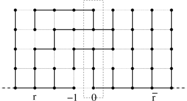
Figure 2: (a) an example of spanning tree $T\in{\mathcal{T}}_{L}$ and its extension in ${\mathcal{T}}_{\infty}$ with the structure at level $0$ put in evidence; (b) extracting the local structure of $T$ at level $0$; c) the corresponding auxiliary graph $G^{\rm aux}_{0,T}$.

One may visualize the elements of $A^{\rm left}$ and $A^{\rm right}$ as being distinct auxiliary vertices “to the left at level $-1$” and “to the right at level $1$”, respectively. For any vertex $v\in V_{0}$ such that there is a horizontal line $v_{-1/2}$ in $T$ connecting it to $(-1,v)$, we draw an auxiliary line from $v$ to the vertex $[v]^{\rm left}$ (a square dot in Figure 2). Similarly, we draw auxiliary lines on the right. In this way, we get a graph $G^{\rm aux}=G^{\rm aux}_{0,T}$ as follows. Its set of vertices is the union of the set $V_{0}$ of vertices at level $0$ together with the new vertices corresponding to the classes in $A^{\rm left}$ and $A^{\rm right}$. Its set of (undirected) edges consists of the forest $F\cap E_{0}$ and the auxiliary lines introduced above. By construction, $G^{\rm aux}_{0,T}$ is a tree; see Figure 2 for an example. We will denote the auxiliary vertex associated to $b^{\rm left}$ on the left (in $G^{\rm aux}_{0,T}$) by $-\infty:=[b^{\rm left}]^{\rm left}$. Similarly, $\infty:=[b^{\rm right}]^{\rm right}$. With these notions, we can define the local tree variables.

Definition 5.2 (Local tree variables)

For any tree $T\in{\mathcal{T}}_{\infty}$, we define its “local tree variable” at level $0$ by

$$\tau=\tau_{0,T}:=(A^{\rm left},b^{\rm left},F,b^{\rm right},A^{\rm right}).$$ (5.3)

We define also its “local tree variable” at level $n\in{\mathbb{Z}}$ by taking the local tree variable at level $0$ of the shifted tree $\theta^{-n}T$:

$$\tau_{n,T}=(A_{n,T}^{\rm left},b_{n,T}^{\rm left},F_{n,T},b_{n,T}^{\rm right},A_{n,T}^{\rm right}):=\tau_{0,\theta^{-n}T}.$$ (5.4)

All other quantities of the form $\operatorname{``something^{\prime\prime}}_{0,T}$ can be generalized to $\operatorname{``something^{\prime\prime}}_{n,T}:=\operatorname{``something^{\prime\prime}}_{0,\theta^{-n}T}$, as well. Both $\tau_{0,T}$ and $\tau_{n,T}$ belong to the set ${\tt treevar}$ defined as follows

$${\tt treevar}=\{\tau_{0,T}:T\in{\mathcal{T}}_{\infty}\}.$$ (5.5)

Note that ${\tt treevar}$ is a finite set since there are only finitely many choices for $A^{{\rm left}/{\rm right}}$, $b^{{\rm left}/{\rm right}}$, and $F$.

The local tree structure near level $n$ can be completely recovered from $\tau_{n,T}$. This is proved in the following theorem.

Theorem 5.3

For all $T\in{\mathcal{T}}_{\infty}$, $n\in{\mathbb{Z}}$, for any given, known edge $e\in E_{-1/2}\cup E_{0}\cup E_{1/2}$, all information we need on its copy $\theta^{n}e$ at level $n$, that is $(a)$ whether it belongs to $T$, $(b)$ if the answer is yes, which end point of $\theta^{n}e$ is closer to $-\infty$ in $T$, hence its orientation in $T$, and $(c)$ whether $\theta^{n}e$ belongs to the backbone $B(T)$ of $T$, can be recovered from knowing $\tau_{n,T}$ without knowing $n$, $T$ or $B(T)$ explicitly. Moreover, the following map is one-to-one.

$$\mathbb{T}:{\mathcal{T}}_{\infty}\to{\tt treevar}^{\mathbb{Z}},\quad\mathbb{T}(T)=(\tau_{n,T})_{n\in{\mathbb{Z}}}$$ (5.6)

The map $\mathbb{T}$ above is not onto (except in the trivial case of the one-dimensional chain ${\mathcal{G}}={\mathbb{Z}}$). To describe its range, we need to introduce a matching condition as follows.

Definition 5.4 (Matching relation for tree variables)

Let $\tau,\tau^{\prime}\in{\tt treevar}$. We say that $\tau$ can be followed by $\tau^{\prime}$, in symbols $\tau\leadsto\tau^{\prime}$, if there is a tree $T\in{\mathcal{T}}_{\infty}$ such that $\tau_{0,T}=\tau$ and $\tau_{1,T}=\tau^{\prime}$. Furthermore, for all $L=(-{\underline{L}},{\overline{L}})$, using the abbreviation $\tau_{\rm bb}=\tau_{0,T^{{\rm bb}}_{\infty}}$, we define

$${\tt words}_{L}:=\{(\tau_{n})_{n\in{\mathbb{Z}}}\in{\tt treevar}^{\mathbb{Z}}:\;\forall n\in{\mathbb{Z}}\;\tau_{n}\leadsto\tau_{n+1}\text{ and }\forall n\in{\mathbb{Z}}\setminus[-{\underline{L}},{\overline{L}}]\;\tau_{n}=\tau_{\rm bb}\}.$$ (5.7)

With this definition we are finally able to reconstruct spanning trees from sequences of local tree variables, as follows.

Theorem 5.5

For any $L$, the function $\mathbb{T}$ maps ${\mathcal{T}}_{L}$ bijectively onto ${\tt words}_{L}$. The map $\mathbb{T}:{\mathcal{T}}_{\infty}\to{\tt words}:=\bigcup_{L}{\tt words}_{L}$ is a bijection. Moreover, there is $N\in{\mathbb{N}}$ such that for all $\tau,\tau^{\prime}\in{\tt treevar}$, there are $\tau_{0},\ldots,\tau_{N}\in{\tt treevar}$ with

$$\tau=\tau_{0}\leadsto\tau_{1}\leadsto\ldots\leadsto\tau_{N}=\tau^{\prime}.$$ (5.8)

We will also need to use some reflection properties of trees. We define a reflection operation $\leftrightarrow:E\to E$, $e\mapsto e^{\leftrightarrow}$ on edges, by $e_{n}^{\leftrightarrow}=e_{-n}$ for any vertical edge $e_{n}\in E_{n}$, $n\in{\mathbb{Z}}$, and $v_{n+1/2}^{\leftrightarrow}=v_{-n-1/2}$ for any horizontal edge $v_{n+1/2}\in E_{n+1/2}$. In the same way, we define a reflection $\leftrightarrow:{\mathcal{T}}_{\infty}\to{\mathcal{T}}_{\infty}$, $T\mapsto T^{\leftrightarrow}$, on trees, by $T^{\leftrightarrow}=\{e^{\leftrightarrow}:\;e\in T\}$. Finally, for any local tree variable $\tau=(b^{\rm left},A^{\rm left},F,A^{\rm right},b^{\rm right})\in{\tt treevar}$, we set $\tau^{\leftrightarrow}=(b^{\rm right},A^{\rm right},F^{\leftrightarrow},A^{\rm left},b^{\rm left})\in{\tt treevar}$, where $F^{\leftrightarrow}=\{e^{\leftrightarrow}:\;e\in F\}$. Note that $\leftrightarrow^{2}=\operatorname{id}$ holds for these reflection operations.

Lemma 5.6

The reflection operation satisfies

$$\tau_{0,T^{\leftrightarrow}}=[\tau_{0,T}]^{\leftrightarrow}\qquad\mbox{and}\qquad\tau\leadsto\tau^{\prime}\ \Leftrightarrow\ (\tau^{\prime})^{\leftrightarrow}\leadsto\tau^{\leftrightarrow}.$$ (5.9)

The rest of this subsection is devoted to the proofs of the above statements. However, in the next section, only the claims of the theorems are used, but no details from the proofs.

5.1.2 Proofs

Proof of Lemma 5.6. Since “left” and “right” are exchanged in the definition of both, $T^{\leftrightarrow}$ and $\tau^{\leftrightarrow}$, the first claim $\tau_{0,T^{\leftrightarrow}}=[\tau_{0,T}]^{\leftrightarrow}$ follows immediately. For the second claim, let $\tau,\tau^{\prime}\in{\tt treevar}$ with $\tau\leadsto\tau^{\prime}$. Then, there exists $T\in{\mathcal{T}}_{\infty}$ with $\tau_{0,T}=\tau$ and $\tau_{1,T}=\tau^{\prime}$. Then the reflected tree satisfies $\tau_{0,T^{\leftrightarrow}}=\tau_{0,T}^{\leftrightarrow}=\tau^{\leftrightarrow}$ and $\tau_{-1,T^{\leftrightarrow}}=\tau_{1,T}^{\leftrightarrow}=(\tau^{\prime})^{\leftrightarrow}$. This shows that $(\tau^{\prime})^{\leftrightarrow}\leadsto\tau^{\leftrightarrow}$.   

Auxiliary finite trees.

Given a tree $T\in{\mathcal{T}}_{\infty}$ and two levels $m,n\in{\mathbb{Z}}$ with $m\leq n$, we define an auxiliary graph $G^{\rm aux}_{[m,n],T}$ as follows. Its set of vertices consists of the union of $\bigcup_{k=m}^{n}V_{k}$ together with a copy $\theta^{m}A^{\rm left}_{m,T}$ of $A^{\rm left}_{m,T}$ formally associated to level $m-1$ and a copy $\theta^{n}A^{\rm right}_{n,T}$ of $A^{\rm right}_{n,T}$ formally associated to level $n+1$. The set of edges in $G^{\rm aux}_{[m,n],T}$ consists of all edges in $T\cap\bigcup_{k\in\frac{{\mathbb{Z}}}{2}\cap[m,n]}E_{k}$ together with an auxiliary line connecting every $(m,v)\in V_{m}$ with $v_{m-1/2}\in T$ to the copy $\theta^{m}[v]^{\rm left}_{m,T}$ of its class $[v]^{\rm left}_{m,T}$, and an auxiliary line connecting every $(n,v)\in V_{n}$ with $v_{n+1/2}\in T$ to the copy $\theta^{n}[v]^{\rm right}_{n,T}$ of its class $[v]^{\rm right}_{n,T}$. Note that $G^{\rm aux}_{[m,n],T}$ is again a spanning tree, and that $G^{\rm aux}_{[n,n],T}=\theta^{n}G^{\rm aux}_{n,T}$ where $G^{\rm aux}_{n,T}=G^{\rm aux}_{0,\theta^{-n}T}$. In particular $G^{\rm aux}_{[0,0],T}=G^{\rm aux}_{0,T}$. See Fig. 3 for an example.

In the following, the word “path” means “simple path”.

       

Figure 3: (a) another example of spanning tree $T\in{\mathcal{T}}_{\infty}$ with the path $\gamma_{T}^{uv}$ in evidence; b) the corresponding auxiliary graph $G^{\rm aux}_{[-1,0],T}$, with $\gamma_{{\rm aux},T}^{uv}$, $(-1,b_{-1,T}^{\rm left})$ and $(0,b_{0,T}^{\rm right})$ in evidence.

Lemma 5.7

Consider two vertices $u,v\in\bigcup_{k=m}^{n}V_{k}$ and the paths $\gamma^{uv}_{T}$ and $\gamma^{uv}_{{\rm aux},T}$ connecting them in $T$ and in $G^{\rm aux}_{[m,n],T}$, respectively. Let $e_{1},\ldots,e_{j}$ be the edges in $\gamma^{uv}_{T}\cap\bigcup_{k\in\frac{{\mathbb{Z}}}{2}\cap[m,n]}E_{k}$, arranged in the order that they are traversed when walking along $\gamma^{uv}_{T}$ from $u$ to $v$. Let $e^{\prime}_{1},\ldots,e^{\prime}_{j^{\prime}}$ be defined similarly, using $G^{\rm aux}_{[m,n],T}$ instead of $T$. Then $(e_{1},\ldots,e_{j})=(e^{\prime}_{1},\ldots,e^{\prime}_{j^{\prime}})$. Moreover, the edges $e_{1},\ldots,e_{j}$ are traversed in the same direction by $\gamma^{uv}_{T}$ and $\gamma^{uv}_{{\rm aux},T}$.

Of particular interest is the case $u=\theta^{m}(b_{m,T}^{\rm left})=(m,b_{m,T}^{\rm left})$ and $v=(n,b_{n,T}^{\rm right})$. In this case, $\gamma^{uv}_{T}$ is the piece of $B(T)$ between $u$ and $v$.

Proof. The proof is straightforward by replacing pieces in $\gamma^{uv}_{T}$ not in $\bigcup_{k\in\frac{{\mathbb{Z}}}{2}\cap[m,n]}E_{k}$ by auxiliary lines. See Fig. 3 for an example.   

Proof of Theorem 5.3. Recall from (5.3) and (5.4) that $\tau_{n,T}$ contains the information $A_{n,T}^{\rm left}$, $b_{n,T}^{\rm left}$, $F_{n,T}$, $b_{n,T}^{\rm right}$, $A_{n,T}^{\rm right}$ and is equivalent to the auxiliary graph $G^{\rm aux}_{n,T}$ with the additional markings “$\pm\infty$”.

(a) For any edge $e\in E_{-1/2}\cup E_{0}\cup E_{1/2}$ we have $\theta^{n}e\in T$ if and only if $e\in F_{n,T}$.

(b) Now assume $\theta^{n}e\in T$. If $e=(b^{\rm left}_{n,T})_{-1/2}$ then $e\in B(\theta^{-n}T)\cap F_{n,T}$, by definition of $b^{{\rm left}}$, which is equivalent to $\theta^{n}e\in B(T)\cap\theta^{n}F_{n,T}$. Then the endpoint $(n-1,b^{\rm left}_{n,T})$ is the one closer to $-\infty$ in $T$. For any other edge $e\in\theta^{-n}T\cap F_{n,T}$, let $u\in V_{0}$ be one endpoint. For a horizontal edge we have $e=u_{\pm 1/2}\in E_{\pm 1/2}$ and the edge corresponds to the auxiliary line connecting $u_{\pm 1/2}$ to $[u]^{{\rm right}/{\rm left}}_{n,T}$ in $G^{\rm aux}_{n,T}$. Consider the path $\gamma$ from $(0,b^{\rm left}_{n,T})$ to $(0,u)$ in $G^{\rm aux}_{n,T}$. Using Lemma 5.7, it follows that $(n,u)$ is the endpoint of $\theta^{n}e$ closer to $-\infty$ in $T$ if and only if the path $\gamma$ does not contain $e$ (or the corresponding auxiliary line).

$(c)$ Using again Lemma 5.7, the edge $e\in E_{-1/2}\cup E_{0}\cup E_{1/2}$ belongs to $B(\theta^{-n}T)\cap F_{n,T}$ if and only if one of the following three cases holds: $e=(b^{\rm left}_{n,T})_{-1/2}$, or $e=(b^{\rm right}_{n,T})_{1/2}$, or $e$ belongs to the path from $b^{\rm left}_{n,T}$ to $b^{\rm right}_{n,T}$ in $G^{\rm aux}_{n,T}$.

Finally, the map $\mathbb{T}$ is one-to-one, because $T=\bigcup_{n\in{\mathbb{Z}}}\theta^{n}F_{n,T}$ holds for all $T\in{\mathcal{T}}_{\infty}$. This concludes the proof.   

When two different trees coincide somewhere, their corresponding local tree variables satisfy the following matching properties.

Lemma 5.8

Let $T,T^{\prime}\in{\mathcal{T}}_{\infty}$ be two trees and $m\in{\mathbb{Z}}$.

1. If $F_{m,T}=F_{m,T^{\prime}}$ and $A_{m,T}^{\rm left}=A_{m,T^{\prime}}^{\rm left}$ hold, then $A_{m+1,T}^{\rm left}=A_{m+1,T^{\prime}}^{\rm left}$ holds as well. Similarly, the assumptions $F_{m+1,T}=F_{m+1,T^{\prime}}$ and $A_{m+1,T}^{\rm right}=A_{m+1,T^{\prime}}^{\rm right}$ imply $A_{m,T}^{\rm right}=A_{m,T^{\prime}}^{\rm right}$.

2. Assume that $G^{\rm aux}_{[m,m+1],T}=G^{\rm aux}_{[m,m+1],T^{\prime}}$, $b_{m,T}^{\rm left}=b_{m,T^{\prime}}^{\rm left}$, and $b_{m+1,T}^{\rm right}=b_{m+1,T^{\prime}}^{\rm right}$ hold. Then $b_{m+1,T}^{\rm left}=b_{m+1,T^{\prime}}^{\rm left}$ and $b_{m,T}^{\rm right}=b_{m,T^{\prime}}^{\rm right}$ hold also.

3. Assume that $F_{n,T}=F_{n,T^{\prime}}$ for all $n\leq m$ and $\tau_{m,T}=\tau_{m,T^{\prime}}$ hold. Then $\tau_{n,T}=\tau_{n,T^{\prime}}$ holds for all $n\leq m$. The same holds when “$n\leq m$” is replaced by “$n\geq m$” in the assumption and in the claim.

Proof. Part 1: Consider a path in $T$ connecting two vertices $u$ and $v$ on level $m+1$ using only edges on levels $\leq m+1/2$. Since $A_{m,T}^{\rm left}=A_{m,T^{\prime}}^{\rm left}$, any excursion in the path from one vertex on level $m$ to another vertex on level $m$ using only edges on levels $\leq m-1/2$ can be replaced by an excursion in $T^{\prime}$ between the same vertices, also using only edges on levels $\leq m-1/2$. In this way, we get a path in $T^{\prime}$ from $u$ to $v$ which uses also only edges on levels $\leq m+1/2$. The same holds when $T$ and $T^{\prime}$ are exchanged. The second statement follows by the same argument, exchanging “left” and “right”. As an example, compare the trees in Fig. 2 and 3 on levels $-1$ and $0$.

Part 2: This follows directly from Lemma 5.7, applied to $u=\theta^{m}b_{m,T}^{\rm left}$ and $v=\theta^{m+1}b_{m+1,T}^{\rm right}$.

Part 3: The assumption $F_{n,T}=F_{n,T^{\prime}}$ for $n\leq m$ implies that $T$ and $T^{\prime}$ coincide on all levels $\leq m+1/2$. It follows that $A^{\rm left}_{n,T}=A^{\rm left}_{n,T^{\prime}}$ and $b^{\rm left}_{n,T}=b^{\rm left}_{n,T^{\prime}}$ hold for $n\leq m$. From this, the first claim in 3. follows by induction over $n$, starting with $n=m$ and using parts 1. and 2. of the lemma in the induction step. The second claim in 3. follows similarly, exchanging the roles of “left” and “right”.   

The next lemma gives criteria to paste pieces of different trees together.

Lemma 5.9 (Glueing trees)

Let $m\in{\mathbb{Z}}$ and let $T_{\rm left},T_{\rm right}\in{\mathcal{T}}_{\infty}$ be spanning trees with $\tau_{m,T_{\rm left}}\leadsto\tau_{m+1,T_{\rm right}}$. Then there is a unique tree $T\in{\mathcal{T}}_{\infty}$, called $\operatorname{glue}_{m}(T_{\rm left},T_{\rm right})$, with $\tau_{n,T}=\tau_{n,T_{\rm left}}$ for $n\leq m$ and $\tau_{n,T}=\tau_{n,T_{\rm right}}$ for $n\geq m+1$.

Proof. Uniqueness follows from the fact that $F_{n,T}$ is a component of $\tau_{n,T}$, and thus

$$T=\bigcup_{n\in{\mathbb{Z}}}\theta^{n}F_{n,T}=\bigcup_{n\leq m}\theta^{n}F_{n,T_{\rm left}}\cup\bigcup_{n\geq m+1}\theta^{n}F_{n,T_{\rm right}}=:\operatorname{glue}_{m}(T_{\rm left},T_{\rm right}).$$ (5.10)

Existence. We take as definition the unique possible choice $T=\operatorname{glue}_{m}(T_{\rm left},T_{\rm right})$ from above. We will prove below this is a spanning tree and $\tau_{n,T}=\tau_{n,T_{\rm left}}$ for all $n\leq m$ and $\tau_{n,T}=\tau_{n,T_{\rm right}}$ for all $n\geq m+1$.

By definition, $T$ agrees with $T_{\rm left}$ on all levels $\leq m$ and with $T_{\rm right}$ on all levels $\geq m+1$, i.e. $T\cap E_{k}=T_{\rm left}\cap E_{k}$ for all $k\in\frac{{\mathbb{Z}}}{2}$ with $k\leq m$ and $T\cap E_{k}=T_{\rm right}\cap E_{k}$ for all $k\in\frac{{\mathbb{Z}}}{2}$ with $k\geq m+1$. Furthermore, from the definition of $T$, $T\cap E_{m+1/2}=(T_{\rm left}\cup T_{\rm right})\cap E_{m+1/2}$. Since $\tau_{m,T_{\rm left}}\leadsto\tau_{m+1,T_{\rm right}}$, there is a tree $T^{\prime}\in{\mathcal{T}}_{\infty}$ with $\tau_{m,T_{\rm left}}=\tau_{m,T^{\prime}}$ and $\tau_{m+1,T_{\rm right}}=\tau_{m+1,T^{\prime}}$. The tree $T^{\prime}$ plays an important role in the remainder of the proof. We have $T_{\rm left}\cap E_{m+1/2}=T^{\prime}\cap E_{m+1/2}=T_{\rm right}\cap E_{m+1/2}$, hence

$$T^{\prime}\cap E_{m+1/2}=T_{\rm left}\cap E_{m+1/2}=T_{\rm right}\cap E_{m+1/2}=T\cap E_{m+1/2}.$$ (5.11)

In the same way we have $A_{m,T_{{\rm left}}}^{{\rm left}}=A_{m,T^{\prime}}^{{\rm left}}$ and $A_{m+1,T_{{\rm right}}}^{{\rm right}}=A_{m+1,T^{\prime}}^{{\rm right}}$.

$T$ is acyclic. We prove this by contradiction. Assume that $T$ contains a cycle $C$. If all edges in $C$ are on levels $\leq m$ (resp. $\geq m+1$), then it is already a cycle in $T_{\rm left}$ (resp. $T_{\rm right}$), a contradiction. Now suppose that $C$ crosses level $m+1/2$ a non-zero even number of times. This path consists of alternating pieces in $T_{\rm left}$ made of edges at levels $\leq m$ and pieces in $T_{\rm right}$ made of edges at levels $\geq m+1$, connected by horizontal lines at level $m+1/2$. Any piece in $T_{\rm left}$ together with the two horizontal lines at level $m+1/2$ attached to it can be replaced by a path in $T^{\prime}$, made of edges on levels $\leq m$ plus the same two horizontal lines. This is true because $A^{\rm left}_{m+1,T_{\rm left}}=A^{\rm left}_{m+1,T^{\prime}}$ by Part 1 of Lemma 5.8 applied to $T_{\rm left}$ and $T^{\prime}$. Similarly any piece in $T_{\rm right}$ together with the two horizontal lines at level $m+1/2$ attached to it can be replaced by a path in $T^{\prime}$, made of edges on levels $\geq m+1$ plus the same two horizontal lines, since $A^{\rm right}_{m,T_{\rm right}}=A^{\rm right}_{m,T^{\prime}}$. Joining these pieces in $T^{\prime}$, we obtain a cycle in $T^{\prime}$, which is impossible.

$T$ connects any two vertices in ${\mathbb{Z}}\times G_{0}$ to each other. First, from the argument just described above we know that any two horizontal edges in $T$ on level $m+1/2$ are connected by a path in $T$ if and only if they are connected in $T^{\prime}$. Since $T^{\prime}$ is a spanning tree, this implies that any two horizontal edges in $T$ on level $m+1/2$ are connected in $T$. Second, for any vertex $(n,u)$ on any level $n\leq m$ there exists at least one horizontal edge on level $m+1/2$ connected to it in $T_{\rm left}$ by a path using only edges on levels $\leq m+1/2$. This path is also a path in $T$. Third, similarly, for any vertex $(n,v)$ on any level $n\geq m+1$ there is a path in $T_{\rm right}$ and hence in $T$ to some horizontal edge on level $m+1/2$. Combining these three arguments the claim follows.

We have shown that $T$ is a spanning tree, therefore $A_{n,T}^{\rm left},A_{n,T}^{\rm right}$ are well defined for all $n\in\mathbb{Z}$. Obviously $A_{m,T}^{\rm left}=A_{m,T_{\rm left}}^{\rm left}=A_{m,T^{\prime}}^{\rm left}$ and $A_{m+1,T}^{\rm right}=A_{m+1,T_{\rm right}}^{\rm right}=A_{m+1,T^{\prime}}^{\rm right}$. Similarly $b_{m,T}^{\rm left}=b_{m,T_{\rm left}}^{\rm left}=b_{m,T^{\prime}}^{\rm left}$, and $b_{m+1,T}^{\rm right}=b_{m+1,T_{\rm right}}^{\rm right}=b_{m+1,T^{\prime}}^{\rm right}$. Then $G^{\rm aux}_{[m,m+1],T}=G^{\rm aux}_{[m,m+1],T^{\prime}}$ and by a straightforward application of parts 1 and 2 of Lemma 5.8 we get $\tau_{m,T}=\tau_{m,T_{\rm left}}$ and $\tau_{m+1,T}=\tau_{m+1,T_{\rm right}}$. Finally, the claims $\tau_{n,T}=\tau_{n,T_{\rm left}}$ for $n\leq m$ and $\tau_{n,T}=\tau_{n,T_{\rm right}}$ for $n\geq m+1$ follow from part 3 of Lemma 5.8.   

Note that if a spanning tree $T\in{\mathcal{T}}_{\infty}$ satisfies $F_{0,T}=F_{0,T^{{\rm bb}}_{\infty}}$, then $\tau_{0,T}=\tau_{0,T^{{\rm bb}}_{\infty}}=\tau_{\rm bb}$. In other words, $\tau_{\rm bb}$ is the only tree variable representing a tree locally at $0$ which looks like $T^{{\rm bb}}_{\infty}$ near $0$. This comes from the fact that $T^{{\rm bb}}_{\infty}$ has only one horizontal line on level $1/2$ and only one on level $-1/2$.

Proof of Theorem 5.5. The map $\mathbb{T}$ is one-to-one by Theorem 5.3. To prove that the map $\mathbb{T}$ is onto, let $\tau=(\tau_{n})_{n\in{\mathbb{Z}}}\in{\tt words}$. We prove by induction that for any $m\in{\mathbb{Z}}$, there is a tree $T^{m}_{\rm left}\in{\mathcal{T}}_{\infty}$ such that $\tau_{n,T^{m}_{\rm left}}=\tau_{n}$ for all $n\in{\mathbb{Z}}$ with $n\leq m$. First, we see that this claim is true for all $m$ sufficiently close to $-\infty$. Indeed, for $m$ so small that $\tau_{n}=\tau_{\rm bb}$ for all $n\leq m$, we can just take $T^{m}_{\rm left}=T^{{\rm bb}}_{\infty}$. For the induction step, assume that the claim holds for a given $m$. Since $\tau\in{\tt words}$, it follows $\tau_{m}\leadsto\tau_{m+1}$. Hence, there is a spanning tree $T_{\rm right}^{m}$ with $\tau_{m,T_{\rm right}^{m}}=\tau_{m}$ and $\tau_{m+1,T_{\rm right}^{m}}=\tau_{m+1}$. Taking $T^{m+1}_{\rm left}:=\operatorname{glue}_{m}(T^{m}_{\rm left},T^{m}_{\rm right})$ from Lemma 5.9, we obtain $\tau_{n,T^{m+1}_{\rm left}}=\tau_{n,T^{m}_{\rm left}}=\tau_{n}$ for all $n\in{\mathbb{Z}}$ with $n\leq m$, and $\tau_{m+1,T^{m+1}_{\rm left}}=\tau_{m+1,T_{\rm right}^{m}}=\tau_{m+1}$. This finishes the inductive proof. Now take $m\in{\mathbb{N}}$ so large that $\tau_{n}=\tau_{\rm bb}$ holds for all $n\geq m$. Using $\tau_{\rm bb}\leadsto\tau_{\rm bb}$, we can take $T:=\operatorname{glue}_{m}(T_{\rm left}^{m},T^{{\rm bb}}_{\infty})$. Then $\mathbb{T}(T)=\tau$.

Next, we prove that for any $L=(-{\underline{L}},{\overline{L}})$, the function $\mathbb{T}$ maps ${\mathcal{T}}_{L}$ onto ${\tt words}_{L}$. For $T\in{\mathcal{T}}_{L}$, note that $\tau_{n,T}=\tau_{\rm bb}$ for all $n\in{\mathbb{Z}}\setminus[-{\underline{L}},{\overline{L}}]$. Consequently, $\mathbb{T}({\mathcal{T}}_{L})\subseteq{\tt words}_{L}$. To prove that $\mathbb{T}({\mathcal{T}}_{L})\supseteq{\tt words}_{L}$, take $\tau\in{\tt words}_{L}$. By the above, there exists $T\in{\mathcal{T}}_{\infty}$ with $\mathbb{T}(T)=\tau$. Since $T=\bigcup_{n\in{\mathbb{Z}}}\theta^{n}F_{n,T}$, the tree $T$ agrees with $T^{{\rm bb}}_{\infty}$ on $({\mathbb{Z}}\setminus[-{\underline{L}},{\overline{L}}])\times G_{0}$. Consequently, $T\in{\mathcal{T}}_{L}$.

It remains to prove that there exists $N\in{\mathbb{N}}$ such that for any tree variables $\tau,\tau^{\prime}\in{\tt treevar}$, there is a tree $T\in{\mathcal{T}}_{\infty}$ with $\tau_{0,T}=\tau$ and $\tau_{N,T}=\tau^{\prime}$.

For any $\tau\in{\tt treevar}$, choose a tree $T_{\tau}$ with $\tau=\tau_{0,T_{\tau}}$. Since the set ${\tt treevar}$ is finite, there is $M\in{\mathbb{N}}$ such that for all $n\in{\mathbb{Z}}$ with $|n|\geq M$ and all $\tau\in{\tt treevar}$, one has $\tau_{n,T_{\tau}}=\tau_{\rm bb}$. Take $N=2M+1$. Given $\tau,\tau^{\prime}\in{\tt treevar}$, the tree $T_{\tau}$ equals $T^{{\rm bb}}_{\infty}$ on all levels $\geq M$, while $\theta^{N}T_{\tau^{\prime}}$ equals $T^{{\rm bb}}_{\infty}$ on all levels $\leq M+1$. Gluing $T_{\tau}$ and $\theta^{N}T_{\tau^{\prime}}$ together at level $M+1/2$, we obtain a tree $T=\operatorname{glue}_{M}(T_{\tau},\theta^{N}T_{\tau^{\prime}})$ which satisfies the claim.   

5.2 Joining gradient and local tree variables

Recall that ${\boldsymbol{\Omega}}_{L}=\Omega_{L}\times{\mathcal{T}}_{L}$ denotes the set of all possible values of $\vec{{\boldsymbol{\omega}}}=(\nabla t_{\rm bb},y_{\rm bb},T)$. In the following we identify $\vec{{\boldsymbol{\omega}}}\in{\boldsymbol{\Omega}}_{L}$ with the set of local gradient and tree variables

$$\vec{{\boldsymbol{\omega}}}\equiv\ (({\boldsymbol{\omega}}_{n})_{n\in{\mathbb{Z}}\cap[-{\underline{L}},{\overline{L}}]},(\omega_{n+1/2})_{n+1/2\in({\mathbb{Z}}+1/2)\cap[-{\underline{L}},{\overline{L}}]})$$ (5.12)

where for $n\in{\mathbb{Z}}\cap[-{\underline{L}},{\overline{L}}]$

$${\boldsymbol{\omega}}_{n}=(\omega_{n},\tau_{n})=((\nabla t^{\rm bb}_{e})_{e\in S_{n}},(y^{\rm bb}_{e})_{e\in S_{n}},\tau_{n}(T))\in{\boldsymbol{\Omega}}_{\rm vert}:={\mathbb{R}}^{S}\times{\mathbb{R}}^{S}\times{\tt treevar},$$ (5.13)

and for $n+1/2\in({\mathbb{Z}}+{1}/{2})\cap[-{\underline{L}},{\overline{L}}]$

$$\omega_{n+1/2}=(\nabla t^{\rm bb}_{p_{n+1/2}},y^{\rm bb}_{p_{n+1/2}})\in\Omega_{\rm hor}.$$ (5.14)

The set ${\boldsymbol{\Omega}}_{\rm vert}$ is the domain of definition for the gradient variables associated to vertical edges in $S$ plus the local tree variables. Using (3.7) and (3.8), we view $\nabla t_{e}$ and $y_{e}$ for any $e\in E_{L}$ in the following as functions of $\vec{{\boldsymbol{\omega}}}$. By Theorem 5.5, there is a bijection between the set of spanning trees ${\mathcal{T}}_{L}$ and the set ${\tt words}_{L}$ consisting of words of local tree variables $(\tau_{n})_{n=-{\underline{L}},\dots,{\overline{L}}}$ with suitable matching conditions. Thus, the set ${\boldsymbol{\Omega}}_{L}$ is identified with the subset ${\boldsymbol{\Omega}}_{L}\subseteq\hat{\boldsymbol{\Omega}}_{L}$ of the set

$$\hat{\boldsymbol{\Omega}}_{L}:={\boldsymbol{\Omega}}_{\rm vert}^{{\mathbb{Z}}\cap[-{\underline{L}},{\overline{L}}]}\times(\Omega_{\rm hor})^{({\mathbb{Z}}+1/2)\cap[-{\underline{L}},{\overline{L}}]}$$ (5.15)

consisting of all $\vec{\boldsymbol{\omega}}$ with

$$\tau_{\rm bb}\leadsto\tau_{-{\underline{L}}}\leadsto\tau_{-{\underline{L}}+1}\leadsto\ldots\leadsto\tau_{\overline{L}}\leadsto\tau_{\rm bb}.$$ (5.16)

With these definitions we can reorganize the interpolated measure in order to set up a transfer operator approach. Recall the definition of $h_{e}$ from (3.33). Using the results of Lemma 3.1, Remark 3.5 and Theorem 5.3, the value $h_{e}(\vec{{\boldsymbol{\omega}}})$ for any edge $e$ (vertical or horizontal) can be written in terms of local variables. More precisely, for a vertical edge $e_{n}$ on an integer level $n\in{\mathbb{Z}}\cap[-{\underline{L}},{\overline{L}}]$, the value $h_{e_{n}}(\vec{\boldsymbol{\omega}})$ depends only on $e\in E_{0}$ and ${\boldsymbol{\omega}}_{n}$, but not explicitly on $n$ or any other component of $\vec{\boldsymbol{\omega}}$ (recall that $\beta_{e_{n}}=\beta_{e_{0}}$ for all $n\in\mathbb{Z}$). Thus we can write for $e\in E_{0}$

$$h_{e_{n}}(\vec{{\boldsymbol{\omega}}})=h_{e}^{\rm vert}({\boldsymbol{\omega}}_{n})$$

for some function $h_{e}^{\rm vert}:{\boldsymbol{\Omega}}_{\rm vert}\to{\mathbb{R}}$. Similarly, for a horizontal edge $v_{n+1/2}$ on a half-integer level $n+1/2\in{\mathbb{Z}}\cap(-{\underline{L}},{\overline{L}})$, the value $h_{v_{n+1/2}}(\vec{\boldsymbol{\omega}})$ depends only on $v\in V_{0}$, ${\boldsymbol{\omega}}_{n}$, $\omega_{n+1/2}$ and ${\boldsymbol{\omega}}_{n+1}$. Thus we write in this case

$$h_{v_{n+1/2}}(\vec{{\boldsymbol{\omega}}})=h_{v}^{\rm hor}({\boldsymbol{\omega}}_{n},\omega_{n+1/2},{\boldsymbol{\omega}}_{n+1}).$$

We set ${\boldsymbol{\Omega}}_{\rm middle}:={\boldsymbol{\Omega}}_{\rm vert}\times\Omega_{\rm hor}\times{\boldsymbol{\Omega}}_{\rm vert}$. For arguments $({\boldsymbol{\omega}},\omega_{\rm hor},{\boldsymbol{\omega}}^{\prime})\in{\boldsymbol{\Omega}}_{\rm middle}$ that cannot be written in the form $({\boldsymbol{\omega}}_{n},\omega_{n+1/2},{\boldsymbol{\omega}}_{n+1})$, we set

$$h_{v}^{\rm hor}({\boldsymbol{\omega}},\omega_{\rm hor},{\boldsymbol{\omega}}^{\prime})=+\infty.$$

Note that this is precisely the case when the tree variable $\tau$ in ${\boldsymbol{\omega}}$ and the tree variable $\tau^{\prime}$ in ${\boldsymbol{\omega}}^{\prime}$ do not fulfill $\tau\leadsto\tau^{\prime}$. Using this extension, we get a well-defined function

$$h_{v}^{\rm hor}:{\boldsymbol{\Omega}}_{\rm middle}\to{\mathbb{R}}\cup\{\infty\}$$

for any $v\in V_{0}$. We define $H_{\rm vert}:{\boldsymbol{\Omega}}_{\rm vert}\to{\mathbb{R}}$ and $H_{\rm hor}:{\boldsymbol{\Omega}}_{\rm middle}\to{\mathbb{R}}\cup\{\infty\}$ by

$$H_{{\rm vert}}=\sum_{e\in E_{0}}h_{e}^{\rm vert},\quad H_{\rm hor}=\sum_{v\in V_{0}}h_{v}^{\rm hor}.$$

With the above abbreviations, we can write for $\vec{\boldsymbol{\omega}}\in\hat{\boldsymbol{\Omega}}_{L}$ the interpolated Hamiltonian defined in (3.32) as

$$H_{L}^{{\mathbf{0}}\ell}(\vec{{\boldsymbol{\omega}}})= \sum_{n\in{\mathbb{Z}}\cap[-{\underline{L}},{\overline{L}}]}H_{\rm vert}({\boldsymbol{\omega}}_{n})+\sum_{n+1/2\in({\mathbb{Z}}+1/2)\cap[-{\underline{L}},{\overline{L}}]}H_{\rm hor}({\boldsymbol{\omega}}_{n},\omega_{n+1/2},{\boldsymbol{\omega}}_{n+1})$$ (5.17)

$$-\frac{1}{2}\sum_{n=-{\underline{L}}}^{-1}\nabla t^{{\rm bb}}_{p_{n+1/2}}+\frac{1}{2}\sum_{n=l}^{{\overline{L}}-1}\nabla t^{{\rm bb}}_{p_{n+1/2}},$$ (5.18)

where $H_{L}^{{\mathbf{0}}\ell}(\vec{{\boldsymbol{\omega}}})=\infty$ holds if and only if $\vec{\boldsymbol{\omega}}\notin{\boldsymbol{\Omega}}_{L}$. Furthermore, we define $H_{\rm middle},H_{\rm middle}^{\pm}:{\boldsymbol{\Omega}}_{\rm middle}\to{\mathbb{R}}\cup\{\infty\}$ as follows. For $({\boldsymbol{\omega}},\omega_{\rm hor},{\boldsymbol{\omega}}^{\prime})\in{\boldsymbol{\Omega}}_{\rm middle}$ with $\omega_{\rm hor}=(\nabla t_{\rm hor},y_{\rm hor})$ we set

$$H_{{\rm middle}}({\boldsymbol{\omega}},\omega_{\rm hor},{\boldsymbol{\omega}}^{\prime}) =\frac{1}{2}H_{\rm vert}({\boldsymbol{\omega}})+H_{\rm hor}({\boldsymbol{\omega}},\omega_{\rm hor},{\boldsymbol{\omega}}^{\prime})+\frac{1}{2}H_{\rm vert}({\boldsymbol{\omega}}^{\prime}),$$ (5.19)

$$H_{{\rm middle}}^{\pm}({\boldsymbol{\omega}},\omega_{\rm hor},{\boldsymbol{\omega}}^{\prime}) =H_{{\rm middle}}({\boldsymbol{\omega}},\omega_{\rm hor},{\boldsymbol{\omega}}^{\prime})\pm\frac{1}{2}\nabla t_{\rm hor}.$$ (5.20)

Finally, we set for ${\boldsymbol{\omega}}=(\omega,\tau)\in{\boldsymbol{\Omega}}_{\rm vert}$,

$$H_{\rm left}({\boldsymbol{\omega}}):=\frac{1}{2}H_{\rm vert}({\boldsymbol{\omega}})+\infty\mathbf{1}_{\{\tau_{\rm bb}\not\leadsto\tau\}},\quad H_{\rm right}({\boldsymbol{\omega}}):=\frac{1}{2}H_{\rm vert}({\boldsymbol{\omega}})+\infty\mathbf{1}_{\{\tau\not\leadsto\tau_{\rm bb}\}}.$$ (5.21)

With these definitions we have the following result.

Lemma 5.10

The interpolated Hamiltonian $H_{L}^{{\mathbf{0}}\ell}:\hat{\boldsymbol{\Omega}}_{L}\to{\mathbb{R}}\cup\{\infty\}$ can be written as

$$H_{L}^{{\mathbf{0}}\ell}(\vec{{\boldsymbol{\omega}}})=H_{\rm left}({\boldsymbol{\omega}}_{-{\underline{L}}})+\sum_{n=-{\underline{L}}}^{-1}H_{\rm middle}^{-}({\boldsymbol{\omega}}_{n},\omega_{n+1/2},{\boldsymbol{\omega}}_{n+1})$$ (5.22)

$$+\sum_{n=0}^{l-1}H_{\rm middle}({\boldsymbol{\omega}}_{n},\omega_{n+1/2},{\boldsymbol{\omega}}_{n+1})+\sum_{n=l}^{{\overline{L}}-1}H_{\rm middle}^{+}({\boldsymbol{\omega}}_{n},\omega_{n+1/2},{\boldsymbol{\omega}}_{n+1})+H_{\rm right}({\boldsymbol{\omega}}_{\overline{L}}).$$

It takes finite values precisely on ${\boldsymbol{\Omega}}_{L}$, represented by the constraint (5.16).

Proof. This is an immediate consequence of the definitions above.   

Reflection Symmetry.

For later use, we define

$${\boldsymbol{\omega}}^{\leftrightarrow}=(\omega,\tau^{\leftrightarrow})\in{\boldsymbol{\Omega}}_{\rm vert}\quad\text{ for }\quad{\boldsymbol{\omega}}=(\omega,\tau)\in{\boldsymbol{\Omega}}_{\rm vert}.$$ (5.23)

Note that the reflection operation changes the orientation in $T$ for the edges along the backbone $B(T)$, but not for the ones along $B^{c}(T)$. Moreover $\beta_{e^{\leftrightarrow}}=\beta_{e}$ for all $e\in E$. Then for $e\in E_{0}$, $v\in V_{0}$, ${\boldsymbol{\omega}},{\boldsymbol{\omega}}^{\prime}\in{\boldsymbol{\Omega}}_{\rm vert}$ and $\omega_{\rm hor}\in\Omega_{\rm hor}$ we see from (3.33)

$$h_{e}^{\rm vert}({\boldsymbol{\omega}}^{\leftrightarrow})=h_{e}^{\rm vert}({\boldsymbol{\omega}}),\quad h_{v}^{\rm hor}({\boldsymbol{\omega}}^{\prime\leftrightarrow},-\omega_{\rm hor},{\boldsymbol{\omega}}^{\leftrightarrow})=h_{v}^{\rm hor}({\boldsymbol{\omega}},\omega_{\rm hor},{\boldsymbol{\omega}}^{\prime}).$$ (5.24)

In particular, by Lemma 5.6 we have

$$h_{v}^{\rm hor}({\boldsymbol{\omega}},\omega_{\rm hor},{\boldsymbol{\omega}}^{\prime})<\infty\ \Leftrightarrow\ \tau\leadsto\tau^{\prime}\ \Leftrightarrow\ {\tau^{\prime}}^{\leftrightarrow}\leadsto\tau^{\leftrightarrow}\ \Leftrightarrow\ h_{v}^{\rm hor}({{\boldsymbol{\omega}}^{\prime}}^{\leftrightarrow},-\omega_{\rm hor},{\boldsymbol{\omega}}^{\leftrightarrow})<\infty.$$ (5.25)

The symmetry properties (5.24) imply for $({\boldsymbol{\omega}},\omega_{\rm hor},{\boldsymbol{\omega}}^{\prime})\in{\boldsymbol{\Omega}}_{\rm middle}$

$$H_{\rm middle}({\boldsymbol{\omega}}^{\prime\leftrightarrow},-\omega_{\rm hor},{\boldsymbol{\omega}}^{\leftrightarrow})=H_{\rm middle}({\boldsymbol{\omega}},\omega_{\rm hor},{\boldsymbol{\omega}}^{\prime}).$$ (5.26)

6 The energy contribution

Theorem 6.1

Take a fixed $G_{0}$ and $\vec{\beta}$. For any $\alpha\in{\mathbb{R}}$, the energy contribution (3.47) satisfies

$$E_{L}^{{\mathbf{0}}\ell}(\alpha)=\ \alpha\,l\,c_{10}\ +\ c_{11}(L,l,\alpha)\ \leq\ \alpha\,l\,c_{10}\ +\ c_{11}^{\max}(\alpha)$$ (6.1)

where $c_{10}>0$ and $c_{11}(L,l,\alpha)\in{\mathbb{R}}$ are constants depending also on $G_{0}$ and $\vec{\beta}$, and

$$c_{11}^{\max}(\alpha):=\sup_{L,l}|c_{11}(L,l,\alpha)|<\infty.$$

The rest of the section is devoted to the proof of this result. In Sect. 5 we introduced local tree variables, replacing the global variable $T$. With these new variables we set up a transfer operator method in Sect. 6.1 below. Finally Sect. 6.2 contains the proof of the theorem.

6.1 Setting up the transfer operator

We endow ${\boldsymbol{\Omega}}_{\rm vert}$ with the reference measure $d{\boldsymbol{\omega}}=\prod_{e\in S}d\nabla t_{e}^{\rm bb}\,dy_{e}^{\rm bb}\,d\tau$, where $d\nabla t_{e}^{\rm bb}$ and $dy_{e}^{\rm bb}$ denote the Lebesgue measure on ${\mathbb{R}}$ and $d\tau$ denotes the counting measure on ${\tt treevar}$. The scalar product on $L^{2}({\boldsymbol{\Omega}}_{\rm vert},d{\boldsymbol{\omega}})$ is defined by

$$\left\langle F,G\right\rangle:=\int_{{\boldsymbol{\Omega}}_{\rm vert}}\overline{F({\boldsymbol{\omega}})}G({\boldsymbol{\omega}})d{\boldsymbol{\omega}}.$$

However, here we are using mostly real functions.

Definition 6.2

We define the integral kernels $k,k^{\pm},\tilde{k}_{\alpha}:{\boldsymbol{\Omega}}_{\rm vert}\times{\boldsymbol{\Omega}}_{\rm vert}\to[0,\infty)$ by

$$k({\boldsymbol{\omega}},{\boldsymbol{\omega}}^{\prime})=\int_{\Omega_{\rm hor}}e^{-H_{{\rm middle}}({\boldsymbol{\omega}},\omega_{\rm hor},{\boldsymbol{\omega}}^{\prime})}d\omega_{\rm hor},\quad k^{\pm}({\boldsymbol{\omega}},{\boldsymbol{\omega}}^{\prime})=\int_{\Omega_{\rm hor}}e^{-H_{{\rm middle}}^{\pm}({\boldsymbol{\omega}},\omega_{\rm hor},{\boldsymbol{\omega}}^{\prime})}d\omega_{\rm hor},$$ (6.2)

$$\mbox{and}\quad\tilde{k}_{\alpha}({\boldsymbol{\omega}},{\boldsymbol{\omega}}^{\prime})=\int_{\Omega_{\rm hor}}\left[\nabla t_{\rm hor}+\alpha\chi(\omega,\omega_{\rm hor},\omega^{\prime})\right]e^{-H_{{\rm middle}}({\boldsymbol{\omega}},\omega_{\rm hor},{\boldsymbol{\omega}}^{\prime})}d\omega_{\rm hor},$$

where $\omega_{\rm hor}=(\nabla t_{\rm hor},y_{\rm hor})$, ${\boldsymbol{\omega}}=(\omega,\tau)$, ${\boldsymbol{\omega}}^{\prime}=(\omega^{\prime},\tau^{\prime})$, the function $\chi$ is given by (3.42) and $\alpha\in{\mathbb{R}}$. We also define two functions $\Psi_{\rm left},\Psi_{\rm right}:{\boldsymbol{\Omega}}_{\rm vert}\to[0,\infty)$ by

$$\Psi_{\rm left}({\boldsymbol{\omega}})=e^{-H_{\rm left}({\boldsymbol{\omega}})}\qquad\mbox{and}\qquad\Psi_{\rm right}({\boldsymbol{\omega}})=e^{-H_{\rm right}({\boldsymbol{\omega}})}.$$ (6.3)

Lemma 6.3

$\Psi_{\rm left}$ and $\Psi_{\rm right}$ belong to $L^{2}({\boldsymbol{\Omega}}_{\rm vert},d{\boldsymbol{\omega}})\setminus\{0\}$. The integral kernels $k$, $k^{\pm}$, and $\tilde{k}_{\alpha}$ belong all to $L^{2}({\boldsymbol{\Omega}}_{\rm vert}\times{\boldsymbol{\Omega}}_{\rm vert},d{\boldsymbol{\omega}}\,d{\boldsymbol{\omega}}^{\prime})$.

Proof. Consider any edge $e$ in ${\mathcal{G}}_{L}$ and any $\vec{\boldsymbol{\omega}}=(\nabla t_{\rm bb},y_{\rm bb},T)\equiv((\omega_{n},\tau_{n})_{n\in{\mathbb{Z}}\cap[-{\underline{L}},{\overline{L}}]}$, $(\omega_{n+1/2})_{n+1/2\in({\mathbb{Z}}+1/2)\cap[-{\underline{L}},{\overline{L}}]})$. We bound the contribution $h_{e}(\vec{\boldsymbol{\omega}})$ to the Hamiltonian from (3.33) as follows from below:

$$h_{e}(\vec{\boldsymbol{\omega}})= \beta_{e}\left[\cosh\nabla t_{e}-1+\frac{y_{e}^{2}}{2}\right]+f_{e,T}(\nabla t_{\rm bb})-\log\frac{\beta_{e}}{2\pi}\mathbf{1}_{\{e\in T\}}$$ (6.4)

$$\geq \frac{\beta_{e}}{2}\left[(\nabla t_{e})^{2}+y_{e}^{2}\right]+f_{e,T}(\nabla t_{\rm bb})-\log\frac{\beta_{e}}{2\pi}\mathbf{1}_{\{e\in T\}}$$ (6.5)

with the linear function $f_{e,T}:\nabla t_{\rm bb}\mapsto\nabla t_{e}^{T}\mathbf{1}_{\{e\in B^{c}(T)\}}-\nabla t_{e}^{{\rm bb}}\mathbf{1}_{\{e\in B^{c}(T^{{\rm bb}})\}}/2$. Given $e$ on an integer level $n$, note that $f_{e,T}(\nabla t_{\rm bb})$ depends only on $\tau_{n,T}$ and linearly on the $\nabla t_{\rm bb}$-components in $\omega_{n}$. Similarly, given $e$ on level $n+1/2$, the value $f_{e,T}(\nabla t_{\rm bb})$ depends only on $\tau_{n,T}$ and linearly on the $\nabla t_{\rm bb}$-components in $(\omega_{n},\omega_{n+1/2},\omega_{n+1})$. Summing over edges and dropping the terms $(\nabla t_{e})^{2}+y_{e}^{2}$ in (6.5) for edges $e\notin T^{{\rm bb}}$, we conclude the following for ${\boldsymbol{\omega}}=(\omega,\tau)$, ${\boldsymbol{\omega}}^{\prime}=(\omega^{\prime},\tau^{\prime})\in{\boldsymbol{\Omega}}_{\rm vert}$ and $\omega_{\rm hor}\in\Omega_{\rm hor}$ with some $\beta$-dependent constants $c_{12}^{\rm vert},c_{12}^{\rm hor}>0$, $c_{13}^{\rm vert},c_{13}^{\rm hor}\in{\mathbb{R}}$ and some linear functions $f^{\rm vert}_{\tau}$ and $f^{\rm hor}_{\tau}$:

$$H_{\rm vert}({\boldsymbol{\omega}}) \geq c_{12}^{\rm vert}\|\omega\|^{2}+f^{\rm vert}_{\tau}(\omega)+c_{13}^{\rm vert},$$ (6.6)

$$H_{\rm hor}({\boldsymbol{\omega}},\omega_{\rm hor},{\boldsymbol{\omega}}^{\prime}) \geq c_{12}^{\rm hor}\|(\omega,\omega_{\rm hor},\omega^{\prime})\|^{2}+f^{\rm hor}_{\tau}(\omega,\omega_{\rm hor},\omega^{\prime})+c_{13}^{\rm hor}.$$ (6.7)

Using the definitions (5.19) and (5.20) of $H_{\rm middle}$ and $H_{\rm middle}^{\pm}$, we get that $e^{-H_{\rm middle}({\boldsymbol{\omega}},\omega_{\rm hor},{\boldsymbol{\omega}}^{\prime})}$ and $e^{-H_{\rm middle}^{\pm}({\boldsymbol{\omega}},\omega_{\rm hor},{\boldsymbol{\omega}}^{\prime})}$ are bounded by a $(\tau,\tau^{\prime})$-dependent Gaussian in the arguments $(\omega,\omega_{\rm hor},\omega^{\prime})$. Integrating over $\omega_{\rm hor}$, square integrability of $k$ and $k^{\pm}$ follows. Similarly, using the definition (5.21) of $H_{\rm left}$ and $H_{\rm right}$, it follows that $\Psi_{\rm left}(\omega)=e^{-H_{\rm left}({\boldsymbol{\omega}})}$ and $\Psi_{\rm right}(\omega)=e^{-H_{\rm right}({\boldsymbol{\omega}})}$ are bounded by $\tau$-dependent Gaussians in $\omega$ and hence square integrable. Since $\chi$ is bounded and $\nabla t_{\rm hor}$ depends linearly on $\omega_{\rm hor}$, square integrability of $\tilde{k}_{\alpha}$ follows by the same argument.   

Definition 6.4

We define the transfer operators $\mathcal{K}$, $\mathcal{K}^{\pm}$, and $\tilde{\mathcal{K}}_{\alpha}$ by

$$\mathcal{K}F({\boldsymbol{\omega}})=\int_{{\boldsymbol{\Omega}}_{\rm vert}}k({\boldsymbol{\omega}},{\boldsymbol{\omega}}^{\prime})F({\boldsymbol{\omega}}^{\prime})\,d{\boldsymbol{\omega}}^{\prime}$$ (6.8)

and similarly for $\mathcal{K}^{\pm}$ and $\tilde{\mathcal{K}}_{\alpha}$ using the integral kernels $k^{\pm}$ and $\tilde{k}_{\alpha}$ instead of $k$.

By Lemma 6.3 above, these transfer operators are Hilbert-Schmidt operators from $L^{2}({\boldsymbol{\Omega}}_{\rm vert},d{\boldsymbol{\omega}})$ to $L^{2}({\boldsymbol{\Omega}}_{\rm vert},d{\boldsymbol{\omega}})$. They satisfy the following properties.

Lemma 6.5

The spectral radii $\lambda$, $\lambda^{\pm}$ of the integral operators $\mathcal{K}$, $\mathcal{K}^{\pm}$, and their adjoints $\mathcal{K}^{*}$, $(\mathcal{K}^{\pm})^{*}$ are strictly positive eigenvalues of the corresponding operator and its adjoint. The corresponding eigenspaces are one-dimensional and spanned by strictly positive functions, denoted by $\Phi_{\rm right}$, $\Phi^{\pm}_{\rm right}$, $\Phi_{\rm left}$, $\Phi^{\pm}_{\rm left}$, respectively. We normalize these functions such that $\left\langle\Phi_{\rm left},\Phi_{\rm right}\right\rangle=1$ and $\left\langle\Phi^{\pm}_{\rm left},\Phi^{\pm}_{\rm right}\right\rangle=1$. Projections to the eigenspaces of $\mathcal{K}$, $\mathcal{K}^{\pm}$ are given by $P\Psi=\left\langle\Phi_{\rm left},\Psi\right\rangle\Phi_{\rm right}$ and $P^{\pm}\Psi=\left\langle\Phi_{\rm left}^{\pm},\Psi\right\rangle\Phi^{\pm}_{\rm right}$, respectively. They fulfill $\mathcal{K}P=P\mathcal{K}=\lambda P$ and

$$\|\mathcal{K}^{m}(\operatorname{id}-P)\|=\|\mathcal{K}^{m}-\lambda^{m}P\|=O(a^{m}\lambda^{m})\text{ as }m\to\infty,$$ (6.9)

$$\|(\mathcal{K}^{\pm})^{m}-(\lambda^{\pm})^{m}P^{\pm}\|=O((a^{\pm})^{m}(\lambda^{\pm})^{m})\text{ as }m\to\infty$$ (6.10)

with some constants $a,a^{\pm}\in[0,1)$.

Proof. From Theorem 5.5, it follows that some power $\mathcal{K}^{N}$ of $\mathcal{K}$ has a strictly positive integral kernel. The same holds for some power of $\mathcal{K}^{\pm}$. Furthermore, the values of the integral kernels $k({\boldsymbol{\omega}},{\boldsymbol{\omega}}^{\prime})$ and $k^{\pm}({\boldsymbol{\omega}},{\boldsymbol{\omega}}^{\prime})$ are strictly positive whenever the tree variables $\tau$ in ${\boldsymbol{\omega}}$ and $\tau^{\prime}$ in ${\boldsymbol{\omega}}^{\prime}$ both equal $\tau_{\rm bb}$. Hence, the lemma follows by the Perron-Frobenius-Jentzsch theory; see appendix.   

We remark that $P$ and $P^{\pm}$ need not be self-adjoint.

6.2 Bound on the energy

Using the transfer operator representation, we can now prove the estimate on the energy term. In the following we abbreviate for $m\in{\mathbb{N}}$:

$$\Psi_{\rm left}^{m}:=((\mathcal{K}^{-})^{m})^{*}\Psi_{\rm left},\quad\Psi_{\rm right}^{m}:=(\mathcal{K}^{+})^{m}\Psi_{\rm right}.$$ (6.11)

We have the following result.

Lemma 6.6

The energy term $E_{L}^{{\mathbf{0}}\ell}(\alpha)$ defined in (3.47) can be written as

$$E_{L}^{{\mathbf{0}}\ell}(\alpha)=\frac{1}{2}\sum_{n=0}^{l-1}\frac{\left\langle\Psi^{\underline{L}}_{{\rm left}},\mathcal{K}^{n}\ \tilde{\mathcal{K}}_{\alpha}\ \mathcal{K}^{l-1-n}\Psi^{{\overline{L}}-l}_{{\rm right}}\right\rangle}{\left\langle\Psi^{{\underline{L}}}_{{\rm left}},\mathcal{K}^{l}\Psi^{{\overline{L}}-l}_{{\rm right}}\right\rangle}.$$ (6.12)

Proof. Using Lemma 5.10, this is just a rewriting of the integral in (3.47) in terms of transfer operators.   

We will prove below that each term in this sum can be written as a leading term independent of $n,$ $l$ and $L$ plus a rest that is summable over $n$ and uniformly bounded in $l$ and $L$. The key estimate is proved in the following lemma.

Lemma 6.7

For any $m,n,m^{\prime},n^{\prime}\in{\mathbb{N}}$, we have

$$\frac{\left\langle\Psi^{m}_{{\rm left}},\mathcal{K}^{n}\tilde{\mathcal{K}}_{\alpha}\mathcal{K}^{n^{\prime}}\Psi^{m^{\prime}}_{{\rm right}}\right\rangle}{\left\langle\Psi^{m}_{{\rm left}},\mathcal{K}^{n+n^{\prime}+1}\Psi^{m^{\prime}}_{{\rm right}}\right\rangle}=\frac{\left\langle\Phi_{\rm left},\tilde{\mathcal{K}}_{\alpha}\Phi_{\rm right}\right\rangle}{\left\langle\Phi_{\rm left},\mathcal{K}\Phi_{\rm right}\right\rangle}+R_{m,n,m^{\prime},n^{\prime}}(\alpha)$$ (6.13)

with a rest term $R_{m,n,m^{\prime},n^{\prime}}(\alpha)$ that fulfills

$$\sup_{m,n,m^{\prime},n^{\prime}\in{\mathbb{N}}}\frac{|R_{m,n,m^{\prime},n^{\prime}}(\alpha)|}{a^{\min\{n,n^{\prime}\}}}<\infty,$$ (6.14)

where $a\in(0,1)$ is taken from Lemma 6.5, and $\left\langle\Phi_{\rm left},\mathcal{K}\Phi_{\rm right}\right\rangle=\lambda$ by construction.

Proof. Since $\Psi_{\rm left}(\omega,\tau_{\rm bb})>0$ for any $\omega\in\Omega_{{\rm vert}}$ and $k^{-}((\omega,\tau_{\rm bb}),(\omega^{\prime},\tau_{\rm bb}))>0$ for any $\omega,\omega^{\prime}$, we have $\|\Psi_{\rm left}^{m}\|>0$ for any $m\geq 0$. Therefore the normalized quantities $\hat{\Psi}^{m}_{\rm left}=\Psi^{m}_{\rm left}/\|\Psi^{m}_{\rm left}\|$ and $\hat{\Phi}^{-}_{\rm left}=\Phi^{-}_{\rm left}/\|\Phi^{-}_{\rm left}\|$ are well defined. Replacing ${\rm left}$ by ${\rm right}$ and $k^{-}$ by $k^{+}$ we also find $\|\Psi_{\rm right}^{m}\|>0$ for any $m\geq 0$, so $\hat{\Psi}_{\rm right}^{m}=\Psi_{\rm right}^{m}/\|\Psi_{\rm right}^{m}\|$ and $\hat{\Phi}^{+}_{\rm right}=\Phi^{+}_{\rm right}/\|\Phi^{+}_{\rm right}\|$ are well defined too. We will work with the normalized operators $\hat{\mathcal{K}}=\lambda^{-1}\mathcal{K}$ and $\hat{\mathcal{K}}_{\alpha}=\lambda^{-1}\tilde{\mathcal{K}}_{\alpha}$. Then

$$\frac{\left\langle\Psi^{m}_{{\rm left}},\mathcal{K}^{n}\tilde{\mathcal{K}}_{\alpha}\mathcal{K}^{n^{\prime}}\Psi^{m^{\prime}}_{{\rm right}}\right\rangle}{\left\langle\Psi^{m}_{{\rm left}},\mathcal{K}^{n+n^{\prime}+1}\Psi^{m^{\prime}}_{{\rm right}}\right\rangle}=\frac{\left\langle\hat{\Psi}^{m}_{{\rm left}},\hat{\mathcal{K}}^{n}\hat{\mathcal{K}}_{\alpha}\hat{\mathcal{K}}^{n^{\prime}}\hat{\Psi}^{m^{\prime}}_{{\rm right}}\right\rangle}{\left\langle\hat{\Psi}^{m}_{{\rm left}},\hat{\mathcal{K}}^{n+n^{\prime}+1}\hat{\Psi}^{m^{\prime}}_{{\rm right}}\right\rangle}$$ (6.15)

Abbreviating $P^{c}=\operatorname{id}-P$, we split the numerator in (6.15) in four pieces:

$$\left\langle\hat{\Psi}^{m}_{{\rm left}},\hat{\mathcal{K}}^{n}\hat{\mathcal{K}}_{\alpha}\hat{\mathcal{K}}^{n^{\prime}}\hat{\Psi}^{m^{\prime}}_{{\rm right}}\right\rangle=\left\langle\hat{\Psi}^{m}_{{\rm left}},P\hat{\mathcal{K}}^{n}\hat{\mathcal{K}}_{\alpha}\hat{\mathcal{K}}^{n^{\prime}}P\hat{\Psi}^{m^{\prime}}_{{\rm right}}\right\rangle+\left\langle\hat{\Psi}^{m}_{{\rm left}},P^{c}\hat{\mathcal{K}}^{n}\hat{\mathcal{K}}_{\alpha}\hat{\mathcal{K}}^{n^{\prime}}P\hat{\Psi}^{m^{\prime}}_{{\rm right}}\right\rangle$$

$$\qquad\qquad+\left\langle\hat{\Psi}^{m}_{{\rm left}},P\hat{\mathcal{K}}^{n}\hat{\mathcal{K}}_{\alpha}\hat{\mathcal{K}}^{n^{\prime}}P^{c}\hat{\Psi}^{m^{\prime}}_{{\rm right}}\right\rangle+\left\langle\hat{\Psi}^{m}_{{\rm left}},P^{c}\hat{\mathcal{K}}^{n}\hat{\mathcal{K}}_{\alpha}\hat{\mathcal{K}}^{n^{\prime}}P^{c}\hat{\Psi}^{m^{\prime}}_{{\rm right}}\right\rangle.$$ (6.16)

Using $P\hat{\mathcal{K}}^{n}=P$ and $\hat{\mathcal{K}}^{n^{\prime}}P=P$, the first piece in the sum equals

$$\left\langle\hat{\Psi}^{m}_{{\rm left}},P\hat{\mathcal{K}}_{\alpha}P\hat{\Psi}^{m^{\prime}}_{{\rm right}}\right\rangle=\left\langle\hat{\Psi}^{m}_{{\rm left}},\Phi_{\rm right}\right\rangle\left\langle\Phi_{\rm left},\hat{\mathcal{K}}_{\alpha}\Phi_{\rm right}\right\rangle\left\langle\Phi_{{\rm left}},\hat{\Psi}^{m^{\prime}}_{\rm right}\right\rangle.$$ (6.17)

In the remainder of this proof, the notation “$b_{n}=O(a^{n})$” means that there is a constant $c<\infty$ such that $\sup_{n\in{\mathbb{N}}}|b_{n}/a^{n}|\leq c$. In particular, it implies that $b_{n}$ is finite for every $n$. Using (6.9), the second term in the sum in (6.2) is bounded by

$$\left|\left\langle\hat{\Psi}^{m}_{{\rm left}},P^{c}\hat{\mathcal{K}}^{n}\hat{\mathcal{K}}_{\alpha}\hat{\mathcal{K}}^{n^{\prime}}P\hat{\Psi}^{m^{\prime}}_{{\rm right}}\right\rangle\right|\leq\|P^{c}\hat{\mathcal{K}}^{n}\|\|\hat{\mathcal{K}}_{\alpha}\|\|P\|=O(a^{n})$$ (6.18)

where the constant in $O(a^{n})$ may depend on $\alpha$, but not on $m,m^{\prime},n,n^{\prime}$. The third and fourth terms fulfill a similar bound with $O(a^{n^{\prime}})$ and $O(a^{n+n^{\prime}})$, respectively, instead of $O(a^{n})$. Then the numerator in (6.15) can be written as

$$\left\langle\hat{\Psi}^{m}_{{\rm left}},\hat{\mathcal{K}}^{n}\hat{\mathcal{K}}_{\alpha}\hat{\mathcal{K}}^{n^{\prime}}\hat{\Psi}^{m^{\prime}}_{{\rm right}}\right\rangle=\left\langle\hat{\Psi}^{m}_{{\rm left}},\Phi_{\rm right}\right\rangle\left\langle\Phi_{\rm left},\hat{\mathcal{K}}_{\alpha}\Phi_{\rm right}\right\rangle\left\langle\Phi_{{\rm left}},\hat{\Psi}^{m^{\prime}}_{\rm right}\right\rangle+O(a^{\min\{n,n^{\prime}\}}).$$ (6.19)

Now, we claim

$$(a)\ \inf_{l,m,m^{\prime}\in{\mathbb{N}}}\left\langle\hat{\Psi}^{m}_{{\rm left}},\hat{\mathcal{K}}^{l}\hat{\Psi}^{m^{\prime}}_{{\rm right}}\right\rangle>0,\qquad(b)\ \inf_{m,m^{\prime}\in{\mathbb{N}}}\left\langle\hat{\Psi}^{m}_{{\rm left}},\Phi_{\rm right}\right\rangle\left\langle\Phi_{\rm left},\hat{\Psi}^{m^{\prime}}_{\rm right}\right\rangle>0.$$ (6.20)

Assuming this is true and combining the estimate (6.19) for the numerator with the fact (6.20)$(a)$ that the denominator is uniformly bounded away from 0, the right-hand side of (6.15) can be written as

$$\left\langle\Phi_{\rm left},\hat{\mathcal{K}}_{\alpha}\Phi_{\rm right}\right\rangle\frac{\left\langle\hat{\Psi}^{m}_{{\rm left}},\Phi_{\rm right}\right\rangle\left\langle\Phi_{{\rm left}},\hat{\Psi}^{m^{\prime}}_{\rm right}\right\rangle}{\left\langle\hat{\Psi}^{m}_{{\rm left}},\hat{\mathcal{K}}^{n+n^{\prime}+1}\hat{\Psi}^{m^{\prime}}_{{\rm right}}\right\rangle}+O(a^{\min\{n,n^{\prime}\}}).$$ (6.21)

To estimate the denominator in the last expression, we use the following bound

$$\sup_{m,m^{\prime}}\left|\left\langle\hat{\Psi}^{m}_{{\rm left}},\hat{\mathcal{K}}^{l}\hat{\Psi}^{m^{\prime}}_{{\rm right}}\right\rangle-\left\langle\hat{\Psi}^{m}_{{\rm left}},\Phi_{\rm right}\right\rangle\left\langle\Phi_{\rm left},\hat{\Psi}^{m^{\prime}}_{{\rm right}}\right\rangle\right|$$ (6.22)

$$\qquad=\sup_{m,m^{\prime}}\left|\left\langle\hat{\Psi}^{m}_{{\rm left}},(\hat{\mathcal{K}}^{l}-P)\hat{\Psi}^{m^{\prime}}_{{\rm right}}\right\rangle\right|\leq\|\hat{\mathcal{K}}^{l}-P\|\leq O(a^{l})$$ (6.23)

with $l=n+n^{\prime}+1$. Note that the proof of this estimate does not use (6.20). The fraction in (6.21) is bounded from above using (6.20)$(a)$ and the fact that $\|\hat{\Psi}_{\rm left}^{m}\|=1=\|\hat{\Psi}_{\rm right}^{m^{\prime}}\|$. Moreover, this fraction is bounded from below by a positive constant using (6.20)$(b)$ and (6.23). These estimates hold uniformly in $m,m^{\prime},n,n^{\prime}$. In particular by (6.23) the reciprocal is estimated as follows

$$\sup_{\begin{subarray}{c}n,n^{\prime}:\\ n+n^{\prime}+1=l\end{subarray}}\sup_{m,m^{\prime}}\left|\frac{\left\langle\hat{\Psi}^{m}_{{\rm left}},\hat{\mathcal{K}}^{n+n^{\prime}+1}\hat{\Psi}^{m^{\prime}}_{{\rm right}}\right\rangle}{\left\langle\hat{\Psi}^{m}_{{\rm left}},\Phi_{\rm right}\right\rangle\left\langle\Phi_{{\rm left}},\hat{\Psi}^{m^{\prime}}_{\rm right}\right\rangle}-1\right|=O(a^{l}).$$ (6.24)

These estimates give (6.13) with the bound (6.14). To complete the proof of the lemma we now prove claim (6.20). Recall that $k((\omega,\tau_{\rm bb}),(\omega^{\prime},\tau_{\rm bb}))>0$, $\hat{\Psi}_{\rm left}^{m}(\omega,\tau_{\rm bb})>0$, and $\hat{\Psi}_{\rm right}^{m^{\prime}}(\omega^{\prime},\tau_{\rm bb})>0$ for all $\omega,\omega^{\prime}$ and $m,m^{\prime}\in{\mathbb{N}}$. It follows

$$\left\langle\hat{\Psi}^{m}_{{\rm left}},\hat{\mathcal{K}}^{l}\hat{\Psi}^{m^{\prime}}_{{\rm right}}\right\rangle>0\qquad\text{ and }\qquad\left\langle\hat{\Psi}^{m}_{{\rm left}},\Phi_{\rm right}\right\rangle\left\langle\Phi_{\rm left},\hat{\Psi}^{m^{\prime}}_{\rm right}\right\rangle>0$$ (6.25)

for all $l,m,m^{\prime}\in{\mathbb{N}}$. Similarly, since $\hat{\Phi}_{\rm left}^{-}>0$ and $\hat{\Phi}_{\rm right}^{+}>0$, for all $l,m,m^{\prime}\in{\mathbb{N}}$ we have

$$\left\langle\hat{\Psi}^{m}_{{\rm left}},\hat{\mathcal{K}}^{l}\hat{\Phi}^{+}_{{\rm right}}\right\rangle>0\qquad\text{ and }\qquad\left\langle\hat{\Phi}^{-}_{{\rm left}},\hat{\mathcal{K}}^{l}\hat{\Psi}^{m^{\prime}}_{{\rm right}}\right\rangle>0.$$ (6.26)

We apply the Perron-Frobenius-Jentzsch theory to $\hat{\mathcal{K}}^{\pm}$. More specifically, we observe first $(P^{-})^{*}\hat{\Psi}_{\rm left}=c^{-}\hat{\Phi}_{\rm left}^{-}$ and $P^{+}\hat{\Psi}_{\rm right}=c^{+}\hat{\Phi}_{\rm right}^{+}$ where $c^{-},c^{+}>0$ since $\left\langle\hat{\Psi}_{\rm left},\hat{\Phi}_{\rm right}^{-}\right\rangle>0$ and $\left\langle\hat{\Phi}_{\rm left}^{+},\hat{\Psi}_{\rm right}\right\rangle>0$. Then, using (6.10) we get

$$\hat{\Psi}^{m}_{{\rm left}}\stackrel{{\scriptstyle m\to\infty}}{{\longrightarrow}}\hat{\Phi}^{-}_{\rm left}\quad\text{and}\quad\hat{\Psi}^{m}_{{\rm right}}\stackrel{{\scriptstyle m\to\infty}}{{\longrightarrow}}\hat{\Phi}^{+}_{\rm right},$$ (6.27)

where the limits are taken with respect to $\|{\cdot}\|$. Thus,

$$\left\langle\hat{\Psi}^{m}_{{\rm left}},\Phi_{\rm right}\right\rangle\stackrel{{\scriptstyle m\to\infty}}{{\longrightarrow}}\left\langle\hat{\Phi}_{{\rm left}}^{-},\Phi_{\rm right}\right\rangle>0\text{ and }\left\langle\Phi_{\rm left},\hat{\Psi}^{m}_{{\rm right}}\right\rangle\stackrel{{\scriptstyle m\to\infty}}{{\longrightarrow}}\left\langle\Phi_{{\rm left}},\hat{\Phi}_{\rm right}^{+}\right\rangle>0.$$ (6.28)

Combining this with (6.25), we get (6.20)(b). Using (6.23), this implies for $l_{0}\in{\mathbb{N}}$ large enough

$$\inf_{l\geq\ l_{0}}\inf_{m,m^{\prime}\in{\mathbb{N}}}\left\langle\hat{\Psi}^{m}_{{\rm left}},\hat{\mathcal{K}}^{l}\hat{\Psi}^{m^{\prime}}_{{\rm right}}\right\rangle>0.$$ (6.29)

We consider a given $l<l_{0}$ next. From (6.26), (6.27), and $\left\langle\hat{\Phi}^{-}_{\rm left},\hat{\mathcal{K}}^{l}\hat{\Phi}_{\rm right}^{+}\right\rangle>0$, we have

$$\inf_{m\in{\mathbb{N}}}\left\langle\hat{\Psi}^{m}_{\rm left},\hat{\mathcal{K}}^{l}\hat{\Phi}_{\rm right}^{+}\right\rangle>0\text{ and }\inf_{m^{\prime}\in{\mathbb{N}}}\left\langle\hat{\Phi}_{\rm left}^{-},\hat{\mathcal{K}}^{l}\hat{\Psi}^{m^{\prime}}_{\rm right}\right\rangle>0.$$ (6.30)

Using this, (6.25), and (6.27) again, we find for our given $l$: $\inf_{m,m^{\prime}\in{\mathbb{N}}}\left\langle\hat{\Psi}^{m}_{{\rm left}},\hat{\mathcal{K}}^{l}\hat{\Psi}^{m^{\prime}}_{{\rm right}}\right\rangle>0$. Combining this with (6.29), the claim (6.20)(a) follows.   

Proof of Theorem 6.1. Combining Lemmas 6.6 and 6.7 above, the energy term $E_{L}^{{\mathbf{0}}\ell}(\alpha)$ defined in (3.47) can be written as

$$E_{L}^{{\mathbf{0}}\ell}(\alpha)= \frac{1}{2}l\frac{\left\langle\Phi_{\rm left},\tilde{\mathcal{K}}_{\alpha}\Phi_{\rm right}\right\rangle}{\left\langle\Phi_{\rm left},\mathcal{K}\Phi_{\rm right}\right\rangle}+\frac{1}{2}\sum_{n=0}^{l-1}R_{{\underline{L}},n,{\overline{L}}-l,l-1-n}(\alpha)$$ (6.31)

where, for any given $\alpha$, the rest

$$\frac{1}{2}\sum_{n=0}^{l-1}R_{{\underline{L}},n,{\overline{L}}-l,l-1-n}(\alpha)=c_{11}(G_{0},\beta,L,l,\alpha)$$ (6.32)

is bounded uniformly in $L$ and $l$ since $0\leq a<1$. Now we claim there is a constant $c_{10}=c_{10}(G_{0},\beta)>0$ such that for all $\alpha\in{\mathbb{R}}$ one has

$$\left\langle\Phi_{\rm left},\tilde{\mathcal{K}}_{\alpha}\Phi_{\rm right}\right\rangle=2\alpha\lambda c_{10}.$$ (6.33)

To prove this we split $\tilde{\mathcal{K}}_{\alpha}=\tilde{\mathcal{K}}_{0}+(\tilde{\mathcal{K}}_{\alpha}-\tilde{\mathcal{K}}_{0})$. We claim

$$\left\langle\Phi_{\rm left},\tilde{\mathcal{K}}_{0}\Phi_{\rm right}\right\rangle=0.$$ (6.34)

This is proved by symmetry. Recall from (5.23) that we set ${\boldsymbol{\omega}}^{\leftrightarrow}=(\nabla t,y,\tau^{\leftrightarrow})\in{\boldsymbol{\Omega}}_{\rm vert}$ for ${\boldsymbol{\omega}}=(\nabla t,y,\tau)\in{\boldsymbol{\Omega}}_{\rm vert}$. From (5.26) it follows for ${\boldsymbol{\omega}},{\boldsymbol{\omega}}^{\prime}\in{\boldsymbol{\Omega}}_{\rm vert}$

$$k({\boldsymbol{\omega}}^{\prime},{\boldsymbol{\omega}})=k({\boldsymbol{\omega}}^{\leftrightarrow},{\boldsymbol{\omega}}^{\prime\leftrightarrow})\quad\text{ and }\quad\tilde{k}_{0}({\boldsymbol{\omega}}^{\prime},{\boldsymbol{\omega}})=-\tilde{k}_{0}({\boldsymbol{\omega}}^{\leftrightarrow},{\boldsymbol{\omega}}^{\prime\leftrightarrow}).$$ (6.35)

Since $k$ is real-valued, the first equation implies that $({\boldsymbol{\omega}},{\boldsymbol{\omega}}^{\prime})\mapsto k({\boldsymbol{\omega}}^{\leftrightarrow},{\boldsymbol{\omega}}^{\prime\leftrightarrow})$ is the integral kernel of the adjoint $\mathcal{K}^{*}$ of $\mathcal{K}$. Consider the “reflected” eigenfunctions $\Phi_{\rm right}^{\leftrightarrow},\Phi_{\rm left}^{\leftrightarrow}:{\boldsymbol{\Omega}}_{\rm vert}\to(0,\infty)$, $\Phi_{\rm right}^{\leftrightarrow}({\boldsymbol{\omega}})=\Phi_{\rm right}({\boldsymbol{\omega}}^{\leftrightarrow})$, $\Phi_{\rm left}^{\leftrightarrow}({\boldsymbol{\omega}})=\Phi_{\rm left}({\boldsymbol{\omega}}^{\leftrightarrow})$. Since the reflection $\leftrightarrow$ leaves the reference measure $d{\boldsymbol{\omega}}$ invariant and $\mathcal{K}\Phi_{\rm right}=\lambda\Phi_{\rm right}$, we get $\mathcal{K}^{*}\Phi_{\rm right}^{\leftrightarrow}=\lambda\Phi_{\rm right}^{\leftrightarrow}$. But the eigenspace $E_{\lambda}(\mathcal{K}^{*})$ is spanned by $\Phi_{\rm left}$, then $\Phi_{\rm right}^{\leftrightarrow}=c\Phi_{\rm left}$ for some constant $c>0$, and therefore $\Phi_{\rm left}^{\leftrightarrow}=c^{-1}\Phi_{\rm right}$. We conclude

$$\left\langle\Phi_{\rm left},\tilde{\mathcal{K}}_{0}\Phi_{\rm right}\right\rangle=\int_{{\boldsymbol{\Omega}}_{\rm vert}}\int_{{\boldsymbol{\Omega}}_{\rm vert}}\Phi_{\rm left}({\boldsymbol{\omega}}^{\leftrightarrow})\tilde{k}_{0}({\boldsymbol{\omega}}^{\leftrightarrow},{\boldsymbol{\omega}}^{\prime\leftrightarrow})\Phi_{\rm right}({\boldsymbol{\omega}}^{\prime\leftrightarrow})\,d{\boldsymbol{\omega}}\,d{\boldsymbol{\omega}}^{\prime}$$ (6.36)

$$\qquad=\left\langle\Phi_{\rm right}^{\leftrightarrow},-\tilde{\mathcal{K}}_{0}\Phi_{\rm left}^{\leftrightarrow}\right\rangle=-\left\langle\Phi_{\rm left},\tilde{\mathcal{K}}_{0}\Phi_{\rm right}\right\rangle.$$ (6.37)

This proves claim (6.34). The contribution of $\tilde{\mathcal{K}}_{\alpha}-\tilde{\mathcal{K}}_{0}$ is given by

$$\left\langle\Phi_{\rm left},(\tilde{\mathcal{K}}_{\alpha}-\tilde{\mathcal{K}}_{0})\Phi_{\rm right}\right\rangle=\alpha\int_{{\boldsymbol{\Omega}}_{\rm middle}}\chi({\boldsymbol{\omega}},\omega_{\rm hor},{\boldsymbol{\omega}}^{\prime})e^{-H_{{\rm middle}}({\boldsymbol{\omega}},\omega_{\rm hor},{\boldsymbol{\omega}}^{\prime})}d{\boldsymbol{\omega}}\,d\omega_{\rm hor}\,d{\boldsymbol{\omega}}^{\prime}=:2\alpha\lambda c_{10}.$$ (6.38)

Note that $c_{10}>0$, because the integrand in (6.38) is nonnegative everywhere and positive on a set of positive measure. This proves claim (6.33). Finally, combining (6.31), (6.32) and (6.33) the proof of the theorem follows.   

7 Putting pieces together

Proof of Theorem 2.1. We prove the estimate for $0<l\leq{\overline{L}}$. The case $-{\underline{L}}\leq l<0$ follows by reflection symmetry. Take any $\eta>0$ and $\alpha\in{\mathbb{R}}$ with $|\alpha|\leq c_{6}\eta$. Using (3.30), (3.31), and Lemma 3.8

$$\ln\mathbb{E}_{\mu_{L}^{{\mathbf{0}}}}\left[e^{\frac{t_{\ell}-t_{{\mathbf{0}}}}{2}}\right]=\ln\mathbb{E}_{\mu_{L}^{{\operatorname{grad}},{\mathbf{0}}}}\left[e^{\frac{t_{\ell}-t_{{\mathbf{0}}}}{2}}\right]=\ln Z_{{\mathbf{0}}\ell}^{L}\leq E_{L}^{{\mathbf{0}}\ell}(\alpha)+S_{L}^{{\mathbf{0}}\ell}(\alpha).$$ (7.1)

Inserting the expression for the internal energy $E_{L}^{{\mathbf{0}}\ell}(\alpha)$ from Theorem 6.1 and the estimate for the entropy term $S_{L}^{{\mathbf{0}}\ell}(\alpha)$ from Theorem 4.1 we conclude

$$\ln\mathbb{E}_{\mu^{{\operatorname{grad}},{\mathbf{0}}}_{L}}\left[e^{\frac{t_{\ell}-t_{{\mathbf{0}}}}{2}}\right]\leq c_{7}\alpha^{2}l+\alpha lc_{10}+c_{11}^{\max}(\alpha)=\alpha(c_{7}\alpha+c_{10})\,l+c_{11}^{\max}(\alpha).$$ (7.2)

Taking $\alpha<0$ such that $|\alpha|<\min\{c_{10}/c_{7},c_{6}\eta\}$, Claim (2.11) follows with $c_{1}=e^{c_{11}^{\max}(\alpha)}$ and ${c_{2}}=-\alpha(c_{7}\alpha+c_{10})>0$.

To prove the second part of the theorem, we notice that, by Theorem 3.2, the variables $(t_{{\mathbf{0}}},s_{\mathbf{0}})$ and $(\nabla t_{{\rm bb}},y_{\rm bb})$ are stochastically independent and the distribution of $(t_{{\mathbf{0}}},s_{\mathbf{0}})$ is independent of $L$. Moreover using (3.7) with $i={\mathbf{0}}$ we can reconstruct any $t_{j}$ knowing only $t_{{\mathbf{0}}}$ and a finite number of variables $\nabla t^{{\rm bb}}_{e}$, independent of $L$, for $L$ large enough. A similar statement holds for the $s_{j}$ using only a finite number of variables $\nabla t^{\rm bb}_{e}$ and $y^{\rm bb}_{e}$. Then any local observable of $(t_{j},s_{j})_{j\in V}$ (i.e. depending only on a finite number of lattice sites) can be written as a local observable of $(t_{{\mathbf{0}}},s_{\mathbf{0}},\nabla t_{{\rm bb}},y_{\rm bb})$ uniformly in $L$ for $L$ large enough. Using the definitions of the previous section, in analogy to Lemma 6.6, the average of any bounded local observable can be written as a ratio of scalar products

$$\mathbb{E}_{\mu_{L}^{{\mathbf{0}}}}[\mathcal{O}]=\frac{\left\langle\hat{\Psi}^{{\underline{L}}-j_{1}}_{{\rm left}},\mathcal{K}_{\mathcal{O}}\ \hat{\Psi}^{{\overline{L}}-j_{2}}_{{\rm right}}\right\rangle}{\left\langle\hat{\Psi}^{{\underline{L}}-j_{1}}_{{\rm left}},\left(\mathcal{K}^{-}\right)^{j_{1}}\left(\mathcal{K}^{+}\right)^{j_{2}}\hat{\Psi}^{{\overline{L}}-j_{2}}_{{\rm right}}\right\rangle},$$ (7.3)

where the operator $\mathcal{K}_{\mathcal{O}}$ depends on the observable and the level indices $j_{1},j_{2}\geq 0$ need to be large enough depending on the choice of $\mathcal{K}_{\mathcal{O}}$. Since $\hat{\Psi}^{m}_{{\rm left}/{\rm right}}\rightarrow\hat{\Phi}^{-/+}_{{\rm left}/{\rm right}}$ as $m\to\infty$ by (6.27), the limit of (7.3) as ${\underline{L}},{\overline{L}}\to\infty$ is well defined. If for $L$ large enough one replaces $j_{1}$ by $j_{1}+n_{1}$ and $j_{2}$ by $j_{2}+n_{2}$ and $\mathcal{K}_{\mathcal{O}}$ by $\mathcal{K}_{-}^{n_{1}}\mathcal{K}_{\mathcal{O}}\mathcal{K}_{+}^{n_{2}}$, the expression (7.3) remains unchanged. This holds also in the limit as ${\underline{L}},{\overline{L}}\to\infty$. Hence, the consistency conditions in Kolmogorov’s extension theorem ensure the limiting measure $\mu^{\mathbf{0}}_{\infty}$ exists. This completes the proof.   

Proof of Corollary 2.2. Let $\tilde{Y}=(\tilde{Y}_{n})_{n\in\mathbb{N}_{0}}$ be the discrete time process associated to VRJP on ${\mathcal{G}}_{\rho}$. Let ${\mathcal{G}}_{\rho,L}$ denote the graph obtained from ${\mathcal{G}}_{L}$ by adding the additional vertex $\rho$ connected by an edge to ${\mathbf{0}}$. For any fixed time $T$, the process $\tilde{Y}$ can jump at most a distance of $T$ away from its starting point. Consequently, the law of $(\tilde{Y}_{n})_{n=0,\ldots,T}$ agrees with the law of the discrete time process $(\tilde{Y}_{n}^{L})_{n=0,\ldots,T}$ associated with the VRJP on ${\mathcal{G}}_{\rho,L}$ for all $L=(-{\underline{L}},{\overline{L}})$ with ${\underline{L}},{\overline{L}}>T$. Thus, by Theorem 2 and the remarks in Sect.  6 of [ST12], the process $(\tilde{Y}_{n})_{n=0,\ldots,T}$ is a mixture of reversible Markov chains with mixing measure given by random weights on the edges $W_{ij}(t,s)=\beta_{ij}e^{t_{i}+t_{j}}$ with $t_{i},t_{j}$ distributed according to $\mu^{\mathbf{0}}_{L}$ with $L$ large enough. Note that the edge weights are strictly positive. In particular, for any finite path $\vec{v}:=(v_{0}=\rho,v_{1},\ldots,v_{T})$ in ${\mathcal{G}}_{\rho}$ starting in $\rho$ and all $L$ with ${\underline{L}},{\overline{L}}>T$, one has

$${\mathbb{P}}((\tilde{Y}_{n})_{n=0,\ldots,T}=\vec{v})=\int{\mathbb{P}}^{W(t,s)}((\tilde{Y}_{n})_{n=0,\ldots,T}=\vec{v})\,d\mu_{\mathbf{0}}^{L}(t,s).$$ (7.4)

Since ${\mathbb{P}}^{W(t,s)}((\tilde{Y}_{n})_{n=0,\ldots,T}=\vec{v})\in[0,1]$ is a bounded observable, Theorem 2.1 implies that the right-hand side of (7.4) equals $\int{\mathbb{P}}^{W(t,s)}((\tilde{Y}_{n})_{n=0,\ldots,T}=\vec{v})\,d\mu^{\mathbf{0}}_{\infty}(t,s)$. The events $\{(\tilde{Y}_{n})_{n=0,\ldots,T}=\vec{v}\}$ together with the empty set are closed under intersections and generate the whole space. This shows that $\tilde{Y}$ is a mixture of reversible Markov chains with mixing measure $\mu^{\mathbf{0}}_{\infty}$. Since all edge weights are strictly positive, one has a mixture of irreducible Markov chains.

To prove positive recurrence, let $x=(|x|=l,v)\in V$ be an arbitrary site and set $\ell:=(l,p)$. By Theorem 3.2, $\nabla t_{\rm bb}$ and $t_{\mathbf{0}}$ are independent. Using this fact and the Cauchy-Schwarz inequality, we get for all $L$ with $-{\underline{L}}\leq l\leq{\overline{L}}$,

$$\mathbb{E}_{\mu_{\mathbf{0}}^{L}}\left[e^{\frac{t_{x}}{4}}\right]=\mathbb{E}_{\mu_{\mathbf{0}}^{L}}\left[e^{\frac{t_{x}-t_{\ell}}{4}}e^{\frac{t_{\ell}-t_{\mathbf{0}}}{4}}e^{\frac{t_{\mathbf{0}}}{4}}\right]\leq\mathbb{E}_{\mu_{\mathbf{0}}^{L}}\left[e^{\frac{t_{x}-t_{\ell}}{2}}\right]^{1/2}\mathbb{E}_{\mu_{\mathbf{0}}^{L}}\left[e^{\frac{t_{\ell}-t_{\mathbf{0}}}{2}}\right]^{1/2}\mathbb{E}_{\mu_{\mathbf{0}}^{L}}\left[e^{\frac{t_{\mathbf{0}}}{4}}\right].$$ (7.5)

It follows from Theorem 3.2 that $\mathbb{E}_{\mu_{\mathbf{0}}^{L}}\left[e^{\frac{t_{\mathbf{0}}}{4}}\right]<\infty$. Since $x$ and $\ell$ are on the same level, $\gamma^{x\ell}_{T^{{\rm bb}}}\subset S_{l}$ and thus

$$\mathbb{E}_{\mu_{\mathbf{0}}^{L}}\left[e^{\frac{t_{x}-t_{\ell}}{2}}\right]\leq\mathbb{E}_{\mu_{\mathbf{0}}^{L}}\Bigg{[}\prod_{e\in\gamma^{x\ell}_{T^{{\rm bb}}}}e^{\frac{|\nabla t^{{\rm bb}}_{e}|}{2}}\Bigg{]}\leq C_{\beta}^{|S|}\mathbb{E}_{\mu_{\mathbf{0}}^{L}}\left[e^{\sum_{e\in\gamma^{x\ell}_{T^{{\rm bb}}}}\frac{\beta_{e}}{2}(\cosh\nabla t^{{\rm bb}}_{e}-1+\frac{y_{e}^{2}}{2})}\right]\leq(2C_{\beta})^{|S|}$$ (7.6)

where $C_{\beta}$ is a constant that depends only on $(\beta_{e})_{e\in S}$ and in the last inequality we used a straightforward generalization of [DSZ10, Lemma 3, eq. (6.2) and (2.10)] to the case of variable $\beta$.

Using Theorem 2.1, we conclude

$$\mathbb{E}_{\mu_{\mathbf{0}}^{L}}\left[e^{\frac{t_{x}}{4}}\right]\leq c_{14}e^{-{c_{2}}\frac{|x|}{2}}$$ (7.7)

with a constant $c_{14}>0$. Then, by monotone convergence, we get

$$\mathbb{E}_{\mu^{\mathbf{0}}_{\infty}}\left[e^{\frac{t_{x}}{4}}\right]=\lim_{M\to\infty}\mathbb{E}_{\mu^{\mathbf{0}}_{\infty}}\left[e^{\frac{t_{x}}{4}}\mathbf{1}_{\{|t_{x}|\leq M\}}\right]=\lim_{M\to\infty}\lim_{L\to\infty}\mathbb{E}_{\mu_{\mathbf{0}}^{L}}\left[e^{\frac{t_{x}}{4}}\mathbf{1}_{\{|t_{x}|\leq M\}}\right]\leq c_{14}e^{-{c_{2}}\frac{|x|}{2}}.$$ (7.8)

Using the exponential Chebyshev inequality and a Borel-Cantelli argument, it follows that $\sum_{x\in V}e^{t_{x}}<\infty$ $\mu^{\mathbf{0}}_{\infty}$-a.s. Consequently, $\mu^{\mathbf{0}}_{\infty}$-a.s. the edge weights are summable

$$\sum_{i\sim j}\beta_{ij}e^{t_{i}+t_{j}}\leq(\max_{ij}\beta_{ij})\sum_{i\in V}e^{t_{i}}\sum_{j\in V}e^{t_{j}}<\infty,$$ (7.9)

and hence we have a mixture of positive recurrent Markov chains.   

Proof of Corollary 2.3. The argument is similar to the one used in Theorem 2.1 in [MR07]. For $(t,s)\in{\mathbb{R}}^{V\times V}$, let ${\mathbb{P}}_{v}^{W(t,s)}$ denote the distribution of the Markovian random walk on ${\mathcal{G}}_{\rho}$ with weights $W_{ij}=W_{ij}(t,s)=\beta_{ij}e^{t_{i}+t_{j}}$ starting at $v\in V\cup\{\rho\}$. This random walk is reversible with a reversible measure given by

$$\pi^{W}_{i}=\sum_{j\sim i}W_{ij},\quad i\in V\cup\{\rho\}.$$ (7.10)

For all $n\in{\mathbb{N}}_{0}$ and $v\in V$, one has

$$\pi^{W}_{\rho}{\mathbb{P}}_{\rho}^{W}(\tilde{Y}_{n}=v)=\pi^{W}_{v}{\mathbb{P}}_{v}^{W}(\tilde{Y}_{n}=\rho).$$ (7.11)

Then for any $\alpha\in(0,1)$

$${\mathbb{P}}_{\rho}^{W}(\tilde{Y}_{n}=v) =\left[\frac{\pi^{W}_{v}}{\pi^{W}_{\rho}}\right]^{\alpha}{\mathbb{P}}_{v}^{W}(\tilde{Y}_{n}=\rho)^{\alpha}\,{\mathbb{P}}_{\rho}^{W}(\tilde{Y}_{n}=v)^{1-\alpha}$$ (7.12)

$$\leq\left[\frac{\pi^{W}_{v}}{\pi^{W}_{\rho}}\right]^{\alpha}=\left[\sum_{i\sim v}\frac{\beta_{iv}}{\varepsilon}e^{t_{i}+t_{v}-t_{\mathbf{0}}}\right]^{\alpha}\leq\frac{\beta_{\max}^{\alpha}}{\varepsilon^{\alpha}}\sum_{i\sim v}e^{\alpha(t_{i}+t_{v}-t_{\mathbf{0}})}.$$ (7.13)

Integrating over $s$ and $t$ with respect to $\mu^{\mathbf{0}}_{\infty}$, as in (1.2), we conclude

$${\mathbb{P}}(\tilde{Y}_{n}=v)=\int{\mathbb{P}}_{\rho}^{W(t,s)}(\tilde{Y}_{n}=v)\,d\mu^{\mathbf{0}}_{\infty}(t,s)\leq\frac{\beta_{\max}^{\alpha}}{\varepsilon^{\alpha}}\sum_{i\sim v}\mathbb{E}_{\mu^{\mathbf{0}}_{\infty}}[e^{\alpha(t_{i}+t_{v}-t_{\mathbf{0}})}].$$ (7.14)

Let $\ell=(m,p)$ be the copy of the pinning point ${\mathbf{0}}$ at the level $m=|v|$ of $v$. Using independence of $t_{\mathbf{0}}$ from the gradient variables (see Theorem 3.2 and Lemma 3.1) and the Cauchy-Schwarz inequality, we get, for any $i\sim v$,

$$\mathbb{E}_{\mu^{\mathbf{0}}_{\infty}}[e^{\alpha(t_{i}+t_{v}-t_{\mathbf{0}})}] =\mathbb{E}_{\mu^{\mathbf{0}}_{\infty}}[e^{\alpha(t_{i}-t_{\ell}+t_{v}-t_{\ell})}e^{2\alpha(t_{\ell}-t_{\mathbf{0}})}e^{\alpha t_{\mathbf{0}}}]$$ (7.15)

$$\leq\mathbb{E}_{\mu^{\mathbf{0}}_{\infty}}[e^{2\alpha(t_{i}-t_{\ell}+t_{v}-t_{\ell})}]^{1/2}\ \mathbb{E}_{\mu^{\mathbf{0}}_{\infty}}[e^{4\alpha(t_{\ell}-t_{\mathbf{0}})}]^{1/2}\ \mathbb{E}_{\mu^{\mathbf{0}}_{\infty}}[e^{\alpha t_{\mathbf{0}}}]$$ (7.16)

Now, setting $\alpha=1/8$, we can use Theorem 2.1, plus the same arguments we used in (7.5) and (7.6) above. We obtain

$$\frac{\beta_{\max}^{\alpha}}{\varepsilon^{\alpha}}\sum_{i\sim v}\mathbb{E}_{\mu^{\mathbf{0}}_{\infty}}[e^{\alpha(t_{i}+t_{v}-t_{\mathbf{0}})}]\ \leq\ c_{3}e^{-c_{4}|v|}$$

for some positive constants $c_{3},c_{4}$. This proves the first claim. The second claim follows with precisely the same Borel-Cantelli argument as in Corollary 2.2 [MR07].   

Appendix A Spectral properties of transfer operators

This appendix reviews the results from the Perron-Frobenius-Jentzsch theory that we need. For more background on this theory, we refer to [Sch74] and [Zaa97].

Let $(\Omega,\mathcal{A},\mu)$ be a $\sigma$-finite measure space and $k:\Omega\times\Omega\to{\mathbb{R}}$ be a measurable function with the following properties:

1. $\int_{\Omega}\int_{\Omega}k(x,y)^{2}\,\mu(dx)\,\mu(dy)<\infty.$

2. $k(x,y)\geq 0$ holds for all $x,y\in\Omega$.

3. There are $S\in\mathcal{A}$ with $\mu(S)>0$ and $\epsilon>0$ such that $k(x,y)\geq\epsilon$ holds for all $x,y\in S$.

4. For $N\in{\mathbb{N}}$ with $N\geq 1$, let $k_{N}:\Omega\times\Omega\to{\mathbb{R}}$ denote the iterated integral kernel, recursively defined by $k_{1}=k$ and $k_{N+1}(x,y)=\int_{\Omega}k_{N}(x,z)k(z,y)\,\mu(dz)$. For some $N\in{\mathbb{N}}$ with $N\geq 1$, the kernel $k_{N}$ is strictly positive.

Let $\mathcal{H}=L^{2}(\Omega,\mathcal{A},\mu;{\mathbb{C}})$ and $\mathcal{K},\mathcal{K}^{*}:\mathcal{H}\to\mathcal{H}$ be the linear operators defined by

$$\mathcal{K}f(x)=\int_{\Omega}k(x,y)f(y)\,\mu(dy),\qquad\mathcal{K}^{*}f(y)=\int_{\Omega}f(x)k(x,y)\,\mu(dx)$$

for $\mu$-a.e. $x\in\Omega$, resp. for $\mu$-a.e. $y\in\Omega$, where $\mathcal{K}^{*}$ is the adjoint operator of $\mathcal{K}$. $\mathcal{K}$ and $\mathcal{K}^{*}$ are Hilbert-Schmidt operators; see e.g. Theorem VI.23 in [RS80]. In particular, they are compact; see e.g. Theorem VI.22(e) in [RS80]. For $z\in{\mathbb{C}}$, let

$$E_{z}(\mathcal{K})=\{f\in\mathcal{H}:\;\mathcal{K}f=zf\},\ \text{and}\ S_{z}(\mathcal{K})=\{f\in\mathcal{H}:\;(\mathcal{K}-z\operatorname{id})^{n}f=0\text{ for some }n\in{\mathbb{N}}\}$$

denote the eigenspace $E_{z}(\mathcal{K})$ and the spectral subspace $S_{z}(\mathcal{K})\supseteq E_{z}(\mathcal{K})$ corresponding to $z$, respectively. The eigenspaces $E_{z}(\mathcal{K}^{*})$ and the spectral subspaces $S_{z}(\mathcal{K}^{*})$ for the adjoint operator are defined in the same way. Let $\rho(\mathcal{K})=\{z\in{\mathbb{C}}:\;\mathcal{K}-z\operatorname{id}:\mathcal{H}\to\mathcal{H}\text{ is bijective}\}$ denote the resolvent set of $\mathcal{K}$, $\sigma(\mathcal{K})={\mathbb{C}}\setminus\rho(\mathcal{K})$ be the spectrum, and let $\lambda=r(\mathcal{K}):=\sup_{z\in\sigma(\mathcal{K})}|z|=\lim_{n\to\infty}\|\mathcal{K}^{n}\|^{1/n}$ be the spectral radius. (Equality of these two representations of $r(\mathcal{K})$ is proven in Lemma VII 3.4 in [DS88].) Then the following holds:

1. $\sigma(\mathcal{K})\setminus\{0\}$ consists of isolated points $z$ with $0<\dim E_{z}(\mathcal{K})<\infty$, which can accumulate at most at $0$. If $\dim\mathcal{H}=\infty$, then $0\in\sigma(\mathcal{K})$.

2. For every $z\in\sigma(\mathcal{K})\setminus\{0\}$, one has $\dim S_{z}(\mathcal{K})=\dim S_{\overline{z}}(\mathcal{K}^{*})<\infty$.

3. $\sigma(\mathcal{K}^{*})=\{\overline{z}:z\in\sigma(\mathcal{K})\}=\sigma(\mathcal{K})$ and $\lambda=r(\mathcal{K})=r(\mathcal{K}^{*})>0$.

4. $\lambda\in\sigma(\mathcal{K})$, and $E_{\lambda}(\mathcal{K})$ contains a $\mu$-a.e. positive function $\Phi_{\rm right}>0$. Similarly, $E_{\lambda}(\mathcal{K}^{*})$ contains a $\mu$-a.e. positive function $\Phi_{\rm left}>0$.

5. Let $N\in{\mathbb{N}}$ with $N\geq 1$, $f,g\in\mathcal{H}$ with $g\geq 0$ ($\mu$-a.e.). If $\mathcal{K}^{N}f=\lambda^{N}f+g$, it follows that $g=0$ ($\mu$-a.e.).

6. $\dim E_{\lambda}(\mathcal{K})=1$ and $\dim E_{\lambda}(\mathcal{K}^{*})=1$.

7. $S_{\lambda}(\mathcal{K})=E_{\lambda}(\mathcal{K})$ and $S_{\lambda}(\mathcal{K}^{*})=E_{\lambda}(\mathcal{K}^{*})$.

8. For every $z\in\sigma(\mathcal{K})$ with $z\neq\lambda$, one has $|z|<\lambda$. Furthermore, one has
   $\sup\{|z|:\;z\in\sigma(\mathcal{K})\setminus\{\lambda\}\}<\lambda$.

9. Let $\Phi_{\rm right}$ and $\Phi_{\rm left}$ from (4) be normalized such that $\langle\Phi_{\rm left},\Phi_{\rm right}\rangle=1$. Set $P:\mathcal{H}\to\mathcal{H}$, $Pf=\langle\Phi_{\rm left},f\rangle\Phi_{\rm right}$. Then $\sigma(\mathcal{K}-\lambda P)\setminus\{0\}=\sigma(\mathcal{K})\setminus\{\lambda,0\}$ and $r(\mathcal{K}-\lambda P)<\lambda$.

10. One has $\lambda^{-n}\mathcal{K}^{n}-P=(\lambda^{-1}\mathcal{K}-P)^{n}$ for all $n\in{\mathbb{N}}$, $n\geq 1$, and $\|\lambda^{-n}\mathcal{K}^{n}-P\|=O(a^{n})\text{ as }n\to\infty$ for any $a<1$ with $r(\mathcal{K}-\lambda P)<\lambda a$. Note that such an $a$ exists because of (9).

Proof. Claim (1). This is the content of a theorem by F. Riesz, proven e.g. as Theorem 7.1 in Chapter VII of [Con90].

Claim (2). For any $z\in{\mathbb{C}}\setminus\{0\}$, the operator $\mathcal{K}-z\operatorname{id}$ is a Fredholm operator with Fredholm index $\operatorname{ind}(\mathcal{K}-z\operatorname{id})=\dim\operatorname{ker}(\mathcal{K}-z\operatorname{id})-\dim\operatorname{ker}(\mathcal{K}-z\operatorname{id})^{*}=0$. This follows from the Fredholm alternative, see e.g. Proposition 3.3 in Chapter XI of [Con90]. Then, for any $n\in{\mathbb{N}}$, $(\mathcal{K}-z\operatorname{id})^{n}$ is a Fredholm operator with Fredholm index $\dim\operatorname{ker}(\mathcal{K}-z\operatorname{id})^{n}-\dim\operatorname{ker}(\mathcal{K}^{*}-\overline{z}\operatorname{id})^{n}=\operatorname{ind}(\mathcal{K}-z\operatorname{id})^{n}=n\operatorname{ind}(\mathcal{K}-z\operatorname{id})=0$ as well; see e.g. Theorem 3.7 in Chapter XI of [Con90]. This implies $\dim S_{z}(\mathcal{K})=\dim S_{\overline{z}}(\mathcal{K}^{*})$. To see that these dimensions are finite, it suffices to show that $\operatorname{ker}(\mathcal{K}-z\operatorname{id})^{n}=\operatorname{ker}(\mathcal{K}-z\operatorname{id})^{n+1}$ holds for some $n\in{\mathbb{N}}$, since this implies $\operatorname{ker}(\mathcal{K}-z\operatorname{id})^{m}=\operatorname{ker}(\mathcal{K}-z\operatorname{id})^{m+1}$ for all $m\geq n$. If the inclusion $\operatorname{ker}(\mathcal{K}-z\operatorname{id})^{n}\subset\operatorname{ker}(\mathcal{K}-z\operatorname{id})^{n+1}$ was strict for all $n\in{\mathbb{N}}$, we could choose for every $n\in{\mathbb{N}}$ some $f_{n}\in\operatorname{ker}(\mathcal{K}-z\operatorname{id})^{n+1}$ with $\|f_{n}\|=1$ and $f_{n}\perp\operatorname{ker}(\mathcal{K}-z\operatorname{id})^{n}$. But then $\mathcal{K}f_{n}=zf_{n}+(\mathcal{K}-z\operatorname{id})f_{n}\in zf_{n}+\operatorname{ker}(\mathcal{K}-z\operatorname{id})^{n}$ has at least distance $|z|$ from the space $\operatorname{ker}(\mathcal{K}-z\operatorname{id})^{n}$. Because $\mathcal{K}f_{m}\in\operatorname{ker}(\mathcal{K}-z\operatorname{id})^{n}$ holds for all $m<n$, it follows that $\|\mathcal{K}f_{n}-\mathcal{K}f_{m}\|\geq|z|$ holds for all $m<n$. This means that the sequence $(\mathcal{K}f_{n})_{n\in{\mathbb{N}}}$ cannot have an accumulation point, contradicting the fact that $\mathcal{K}$ is a compact operator.

Claim (3). The first equality is contained in Theorem VI.7 in [RS80]. The second equality follows from the fact that the integral kernel $k$ is real-valued. The claim $r(\mathcal{K})=r(\mathcal{K}^{*})$ follows immediately from $\sigma(\mathcal{K})=\sigma(\mathcal{K}^{*})$. To prove $r(\mathcal{K})>0$, we use hypotheses (b) and (c) as follows: $\mathcal{K}\mathbf{1}_{S}\geq a\mathbf{1}_{S}$, where we abbreviate $a=\epsilon\mu(S)>0$. Because of $k\geq 0$, the operator $\mathcal{K}$ is positive in the sense that $f\geq g$ implies $\mathcal{K}f\geq\mathcal{K}g$ for any $f,g\in\mathcal{H}$. Inductively, it follows that $\mathcal{K}^{n}\mathbf{1}_{S}\geq a^{n}\mathbf{1}_{S}$ holds for all $n\in{\mathbb{N}}$. This implies $\|\mathcal{K}^{n}\|\geq a^{n}$ for all $n$ and hence $r(\mathcal{K})=\lim_{n\to\infty}\|\mathcal{K}^{n}\|^{1/n}\geq a>0$.

Claim (4). Since $\sigma(\mathcal{K})$ is nonempty and compact, there is a $z\in\sigma(\mathcal{K})$ with $|z|=r(\mathcal{K})$. By part (1), there is an eigenfunction $g\in E_{z}(\mathcal{K})$ with $\|g\|=1$. We abbreviate $f:=|g|$. In particular, $\|f\|=\|g\|=1$. From positivity of $\mathcal{K}$, it follows that $\mathcal{K}f=\mathcal{K}|g|\geq|\mathcal{K}g|=|z||g|=\lambda f\geq 0$ and then $\mathcal{K}^{n+1}f\geq\lambda\mathcal{K}^{n}f\geq\lambda^{n+1}f\geq 0$ for all $n\in{\mathbb{N}}$ by iteration. Take a sequence $(\lambda_{m})_{m\in{\mathbb{N}}}$ of positive numbers $\lambda_{m}>\lambda$ with $\lambda_{m}\downarrow\lambda$ as $m\to\infty$ and consider for the moment a fixed $m\in{\mathbb{N}}$. Since $\|\mathcal{K}^{n}f\|\leq\|\mathcal{K}^{n}\|=(\lambda+o(1))^{n}$ as $n\to\infty$, the series

$$h_{m}:=(\operatorname{id}-\lambda_{m}^{-1}\mathcal{K})^{-1}f=\sum_{n=0}^{\infty}\lambda_{m}^{-n}\mathcal{K}^{n}f$$ (A.1)

converges. The facts $f\neq 0$ and $\mathcal{K}^{n}f\geq 0$ for all $n$ imply $h_{m}\neq 0$ and $h_{m}\geq 0$; hence $v_{m}:=h_{m}/\|h_{m}\|\geq 0$ is well-defined. Furthermore,

$$h_{m}\geq\sum_{n=0}^{\infty}\lambda_{m}^{-n}\lambda^{n}f=(1-\lambda/\lambda_{m})^{-1}f\geq 0$$

implies $\|h_{m}\|\geq(1-\lambda/\lambda_{m})^{-1}\|f\|=(1-\lambda/\lambda_{m})^{-1}\stackrel{{\scriptstyle m\to\infty}}{{\longrightarrow}}\infty.$ From $\mathcal{K}h_{m}-\lambda_{m}h_{m}=-\lambda_{m}f$ we conclude $\|\mathcal{K}v_{m}-\lambda_{m}v_{m}\|=\lambda_{m}\|f\|/\|h_{m}\|\to 0$ as $m\to\infty$. Because of $\|\lambda_{m}v_{m}-\lambda v_{m}\|=\lambda_{m}-\lambda\to 0$ it follows also $\|\mathcal{K}v_{m}-\lambda v_{m}\|\to 0$ as $m\to\infty$. In particular, $\lim_{m\to\infty}\|\mathcal{K}v_{m}\|=\lim_{m\to\infty}\|\lambda v_{m}\|=\lambda$. By compactness of the operator $\mathcal{K}$ and $\|v_{m}\|=1$, some subsequence $(\mathcal{K}v_{m_{l}})_{l\in{\mathbb{N}}}$ converges to some $\Phi_{\rm right}\in\mathcal{H}$. By the positivity of $\mathcal{K}$ and $v_{m}\geq 0$ we know $\mathcal{K}v_{m}\geq 0$ for all $m$, hence $\Phi_{\rm right}\geq 0$ ($\mu$-a.e.). Furthermore, $\|\Phi_{\rm right}\|=\lim_{l\to\infty}\|\mathcal{K}v_{m_{l}}\|=\lambda$ and

$$\|\mathcal{K}\Phi_{\rm right}-\lambda\Phi_{\rm right}\|=\lim_{l\to\infty}\|\mathcal{K}^{2}v_{m_{l}}-\lambda\mathcal{K}v_{m_{l}}\|\leq\lim_{l\to\infty}\|\mathcal{K}\|\|\mathcal{K}v_{m_{l}}-\lambda v_{m_{l}}\|=0.$$

This means that $0\neq\Phi_{\rm right}\in E_{\lambda}(\mathcal{K})$, hence $\lambda\in\sigma(\mathcal{K})$. By hypothesis (d), for some $N\in{\mathbb{N}}$ the integral kernel $k_{N}$ of $\mathcal{K}^{N}$ takes only positive values, then the facts $\Phi_{\rm right}\geq 0$, $\Phi_{\rm right}\neq 0$ and $\Phi_{\rm right}=\lambda^{-N}\mathcal{K}^{N}\Phi_{\rm right}$ imply $\Phi_{\rm right}>0$ (modulo changes on null sets). The same arguments, applied to $\mathcal{K}^{*}$ instead of $\mathcal{K}$, show that $E_{\lambda}(\mathcal{K}^{*})$ contains a positive function $\Phi_{\rm left}$ (modulo changes on null sets).

Claim (5). Take $N\in{\mathbb{N}}$, $f,g\in\mathcal{H}$ with $g\geq 0$ $\mu$-a.e. and $\mathcal{K}^{N}f=\lambda^{N}f+g$. Using the eigenfunction $\Phi_{\rm left}>0$ of $\mathcal{K}^{*}$ from Claim (4), we obtain

$$\lambda^{N}\langle\Phi_{\rm left},f\rangle=\langle(\mathcal{K}^{*})^{N}\Phi_{\rm left},f\rangle=\langle\Phi_{\rm left},\mathcal{K}^{N}f\rangle=\lambda^{N}\langle\Phi_{\rm left},f\rangle+\langle\Phi_{\rm left},g\rangle$$

and therefore $\langle\Phi_{\rm left},g\rangle=0$. Since $\Phi_{\rm left}>0$ and $g\geq 0$, this implies $g=0$ $\mu$-a.e.

Claim (6). Let $u\in E_{\lambda}(\mathcal{K})$: our goal is to show that $u$ is a multiple of $\Phi_{\rm right}$ $\mu$-a.e. Take again $N\in{\mathbb{N}}$ as in hypothesis (d); then $u\in E_{\lambda^{N}}(\mathcal{K}^{N})$ also holds. Since the integral kernel $k_{N}$ of $\mathcal{K}^{N}$ is real-valued, it follows $\operatorname{Re}u\in E_{\lambda^{N}}(\mathcal{K}^{N})$ and $\operatorname{Im}u\in E_{\lambda^{N}}(\mathcal{K}^{N})$; thus it suffices to show that every real-valued $u\in E_{\lambda^{N}}(\mathcal{K}^{N})$ is a multiple of $\Phi_{\rm right}$ $\mu$-a.e. Assume by contradiction that this was false. Then there is $a\in{\mathbb{R}}$ such that neither $au+\Phi_{\rm right}\geq 0$ nor $au+\Phi_{\rm right}\leq 0$ holds $\mu$-a.e. Setting $h=au+\Phi_{\rm right}\in E_{\lambda^{N}}(\mathcal{K}^{N})$, $f=|h|$ and $g=\mathcal{K}^{N}|h|-|\mathcal{K}^{N}h|$, it follows $g\geq 0$, and $\mathcal{K}^{N}f=|\mathcal{K}^{N}h|+g=|\lambda^{N}h|+g=\lambda^{N}f+g$. Since the integral kernel $k^{N}$ of $\mathcal{K}^{N}$ takes only positive values, $g$ cannot be $0$ $\mu$-a.e. This contradicts Claim (5).

Claim (7). Assume that there was a strict inclusion $E_{\lambda}(\mathcal{K})\subsetneqq S_{\lambda}(\mathcal{K})$. Then there is $f\in\ker(\mathcal{K}-\lambda\operatorname{id})^{2}$ with $\mathcal{K}f=\lambda f+\Phi_{\rm right}$, since $\ker(\mathcal{K}-\lambda\operatorname{id})=E_{\lambda}(\mathcal{K})$ is spanned by $\Phi_{\rm right}$ by claims (4) and (6). This contradicts Claim (5) since $\Phi_{\rm right}>0$. The same argument applied to $\mathcal{K}^{*}$ instead of $\mathcal{K}$ shows $E_{\lambda}(\mathcal{K}^{*})=S_{\lambda}(\mathcal{K}^{*})$.

Claim (8). Let $z\in\sigma(\mathcal{K})$ with $|z|=\lambda$. Then, by (1), there is an eigenfunction $f\in E_{z}(\mathcal{K})$, $f\neq 0$. Taking $N\in{\mathbb{N}}$ from hypothesis (d), we get $\lambda^{N}|f|=|z^{N}f|=|\mathcal{K}^{N}f|\leq\mathcal{K}^{N}|f|$, by (5) $\lambda^{N}|f|=|\mathcal{K}^{N}f|=\mathcal{K}^{N}|f|$ $\mu$-a.e.. This means for $\mu$-a.e. $x\in\Omega$

$$|\mathcal{K}^{N}f(x)|=\left|\int_{\Omega}k_{N}(x,y)f(y)\,\mu(dy)\right|=\int_{\Omega}k_{N}(x,y)|f(y)|\,\mu(dy)=\mathcal{K}^{N}|f|(x),$$

therefore, again for $\mu$-a.e. $x\in\Omega$, there is a constant $c_{x}\in{\mathbb{C}}$ with $|c_{x}|=1$ such that $k_{N}(x,y)f(y)=c_{x}k_{N}(x,y)|f(y)|$ holds for $\mu$-a.e. $y\in\Omega$. Using that $k_{N}$ is strictly positive, this implies $f=c|f|$ ($\mu$-a.e.) for some $c\in{\mathbb{C}}$ with $|c|=1$, therefore $\mathcal{K}^{N}f=c\mathcal{K}^{N}|f|=c\lambda^{N}|f|=\lambda^{N}f$. We obtain $f\in S_{\lambda}(\mathcal{K})$ and hence $f\in E_{\lambda}(\mathcal{K})$ from Claim (7). This implies $z=\lambda$ since $0\neq f\in E_{z}(\mathcal{K})\cap E_{\lambda}(\mathcal{K})$. This shows that for all $z\in\sigma(\mathcal{K})$ we have $z=\lambda$ or $|z|<\lambda$. Since the spectral values of $\mathcal{K}$ can only accumulate at $0$, this implies $\sup\{|z|:\;z\in\sigma(\mathcal{K})\setminus\{\lambda\}\}<\lambda$.

Claim (9). Let $\Sigma:=\mathcal{K}-\lambda P$. $\Sigma$ is a compact operator, since $\mathcal{K}$ is compact and $P$ has rank $1$. We show now that $\lambda\notin\sigma(\Sigma)$. Let $f\in E_{\lambda}(\Sigma)$; we need to show $f=0$. From

$$\mathcal{K}f-\lambda f =\mathcal{K}f-\Sigma f=\lambda Pf=P\Sigma f=\left\langle\Phi_{\rm left},\mathcal{K}f\right\rangle\Phi_{\rm right}-\lambda\left\langle\Phi_{\rm left},Pf\right\rangle\Phi_{\rm right}$$ (A.2)

$$=\left\langle\mathcal{K}^{*}\Phi_{\rm left},f\right\rangle\Phi_{\rm right}-\lambda\left\langle\Phi_{\rm left},\Phi_{\rm right}\right\rangle\left\langle\Phi_{\rm left},f\right\rangle\Phi_{\rm right}$$ (A.3)

$$=\lambda\left\langle\Phi_{\rm left},f\right\rangle\Phi_{\rm right}-\lambda\left\langle\Phi_{\rm left},f\right\rangle\Phi_{\rm right}=0$$ (A.4)

we get that $f$ is a multiple $c\Phi_{\rm right}$ of $\Phi_{\rm right}$, with $c\in{\mathbb{C}}$, since $E_{\lambda}(\mathcal{K})$ is spanned by $\Phi_{\rm right}$. But $f\in E_{\lambda}(\Sigma)$ and $\Sigma\Phi_{\rm right}=\mathcal{K}\Phi_{\rm right}-\lambda\left\langle\Phi_{\rm left},\Phi_{\rm right}\right\rangle\Phi_{\rm right}=\lambda\Phi_{\rm right}-\lambda\Phi_{\rm right}=0$ then imply $\lambda f=\Sigma f=c\Sigma\Phi_{\rm right}=0$ and therefore $f=0$.

Next, let $z\in{\mathbb{C}}\setminus\{0,\lambda\}$. We need to show that $z\in\sigma(\mathcal{K})$ holds if and only if $z\in\sigma(\Sigma)$. Now every non-zero spectral value of $\mathcal{K}$ (resp. $\Sigma$) is an eigenvalue of $\mathcal{K}$ (resp. $\Sigma$).Therefore, it suffices to show that $E_{z}(\mathcal{K})=E_{z}(\Sigma)$. To prove $E_{z}(\mathcal{K})\subseteq E_{z}(\Sigma)$, let $f\in E_{z}(\mathcal{K})$. Then $\lambda Pf=\lambda\left\langle\Phi_{\rm left},f\right\rangle\Phi_{\rm right}=\left\langle\mathcal{K}^{*}\Phi_{\rm left},f\right\rangle\Phi_{\rm right}=\left\langle\Phi_{\rm left},\mathcal{K}f\right\rangle\Phi_{\rm right}=z\left\langle\Phi_{\rm left},f\right\rangle\Phi_{\rm right}=zPf$, hence $Pf=0$ since $z\neq\lambda$. This shows $\Sigma f=\mathcal{K}f=zf$, i.e. $f\in E_{z}(\Sigma)$.

To prove $E_{z}(\mathcal{K})\supseteq E_{z}(\Sigma)$, let $f\in E_{z}(\Sigma)$. Note that $P^{2}=P$ since for $g\in\mathcal{H}$ we have $P^{2}g=\left\langle\Phi_{\rm left},g\right\rangle\left\langle\Phi_{\rm left},\Phi_{\rm right}\right\rangle\Phi_{\rm right}=\left\langle\Phi_{\rm left},g\right\rangle\Phi_{\rm right}=Pg$. We obtain

$$zPf =P\Sigma f=P\mathcal{K}f-\lambda P^{2}f=\left\langle\Phi_{\rm left},\mathcal{K}f\right\rangle\Phi_{\rm right}-\lambda Pf$$ (A.5)

$$=\left\langle\mathcal{K}^{*}\Phi_{\rm left},f\right\rangle\Phi_{\rm right}-\lambda Pf=\lambda\left\langle\Phi_{\rm left},f\right\rangle\Phi_{\rm right}-\lambda Pf=0$$ (A.6)

hence again $Pf=0$. This shows $\mathcal{K}f=\Sigma f=zf$, i.e. $f\in E_{z}(\mathcal{K})$. Thus we have proven $\sigma(\Sigma)\setminus\{0\}=\sigma(\mathcal{K})\setminus\{\lambda,0\}$. The remaining claim $r(\Sigma)<\lambda$ follows now from assertion (8).

Claim (10). Note that $P\Sigma=0=\Sigma P$ hold, because for $f\in\mathcal{H}$, we have

$$P\Sigma f=\left\langle\Phi_{\rm left},\mathcal{K}f\right\rangle\Phi_{\rm right}-\lambda P^{2}f=\left\langle\mathcal{K}^{*}\Phi_{\rm left},f\right\rangle\Phi_{\rm right}-\lambda Pf=\lambda\left\langle\Phi_{\rm left},f\right\rangle\Phi_{\rm right}-\lambda Pf=0,$$

$$\Sigma Pf=\mathcal{K}Pf-\lambda P^{2}f=\left\langle\Phi_{\rm left},f\right\rangle\mathcal{K}\Phi_{\rm right}-\lambda Pf=\lambda\left\langle\Phi_{\rm left},f\right\rangle\Phi_{\rm right}-\lambda Pf=0.$$

As a consequence, we obtain Claim (10) as follows:

$$\lambda^{-n}\mathcal{K}^{n}=(\lambda^{-1}\Sigma+P)^{n}=\lambda^{-n}\Sigma^{n}+P^{n}=\lambda^{-n}\Sigma^{n}+P=(\lambda^{-1}\mathcal{K}-P)^{n}+P$$

and $\|\lambda^{-n}\mathcal{K}^{n}-P\|^{1/n}=\|\lambda^{-n}\Sigma^{n}\|^{1/n}\stackrel{{\scriptstyle n\to\infty}}{{\longrightarrow}}r(\lambda^{-1}\Sigma)=\lambda^{-1}r(\Sigma)<1.$

References

- [BS12] A.-L. Basdevant and A. Singh. Continuous-time vertex reinforced jump processes on Galton-Watson trees. Ann. Appl. Probab., 22(4):1728–1743, 2012.
- [CD86] D. Coppersmith and P. Diaconis. Random walk with reinforcement. Unpublished manuscript, 1986.
- [Col06] A. Collevecchio. On the transience of processes defined on Galton-Watson trees. Ann. Probab., 34(3):870–878, 2006.
- [Col09] A. Collevecchio. Limit theorems for vertex-reinforced jump processes on regular trees. Electron. J. Probab., 14:no. 66, 1936–1962, 2009.
- [Con90] J.B. Conway. A course in functional analysis, volume 96 of Graduate Texts in Mathematics. Springer-Verlag, New York, second edition, 1990.
- [DFZ92] W. Drunk, D. Fuchs, and M.R. Zirnbauer. Migdal-Kadanoff renormalization of a nonlinear supervector model with hyperbolic symmetry. Ann. Physik (8), 1(2):134–150, 1992.
- [DS88] N. Dunford and J.T. Schwartz. Linear operators. Part I. Wiley Classics Library. John Wiley & Sons Inc., New York, 1988. General theory, With the assistance of William G. Bade and Robert G. Bartle, Reprint of the 1958 original, A Wiley-Interscience Publication.
- [DS10] M. Disertori and T. Spencer. Anderson localization for a supersymmetric sigma model. Comm. Math. Phys., 300(3):659–671, 2010.
- [DSZ10] M. Disertori, T. Spencer, and M.R. Zirnbauer. Quasi-diffusion in a 3D supersymmetric hyperbolic sigma model. Comm. Math. Phys., 300(2):435–486, 2010.
- [DV02] B. Davis and S. Volkov. Continuous time vertex-reinforced jump processes. Probab. Theory Related Fields, 123(2):281–300, 2002.
- [DV04] B. Davis and S. Volkov. Vertex-reinforced jump processes on trees and finite graphs. Probab. Theory Related Fields, 128(1):42–62, 2004.
- [Efe83] K.B. Efetov. Supersymmetry and theory of disordered metals. Adv. in Phys., 32(1):53–127, 1983.
- [Efe97] K. Efetov. Supersymmetry in Disorder and Chaos. Cambridge University Press, 1997.
- [Fyo02] Y.V. Fyodorov. Negative moments of characteristic polynomials of random matrices: Ingham-Siegel integral as an alternative to Hubbard-Stratonovich transformation. Nuclear Phys. B, 621(3):643–674, 2002.
- [KR00] M.S. Keane and S.W.W. Rolles. Edge-reinforced random walk on finite graphs. In Infinite dimensional stochastic analysis (Amsterdam, 1999), pages 217–234. R. Neth. Acad. Arts Sci., Amsterdam, 2000.
- [Mir00a] A.D. Mirlin. Statistics of energy levels and eigenfunctions in disordered and chaotic systems: supersymmetry approach. In New directions in quantum chaos (Villa Monastero, 1999), volume 143 of Proc. Internat. School Phys. Enrico Fermi, pages 223–298. IOS, Amsterdam, 2000.
- [Mir00b] A.D. Mirlin. Statistics of energy levels and eigenfunctions in disordered systems. Phys. Rep., 326(5-6):259–382, 2000.
- [MR05] F. Merkl and S.W.W. Rolles. Edge-reinforced random walk on a ladder. Ann. Probab., 33(6):2051–2093, 2005.
- [MR07] F. Merkl and S.W.W. Rolles. Asymptotic behavior of edge-reinforced random walks. Ann. Probab., 35(1):115–140, 2007.
- [MR09a] F. Merkl and S.W.W. Rolles. Edge-reinforced random walk on one-dimensional periodic graphs. Probab. Theory Related Fields, 145(3-4):323–349, 2009.
- [MR09b] F. Merkl and S.W.W. Rolles. Recurrence of edge-reinforced random walk on a two-dimensional graph. Ann. Probab., 37(5):1679–1714, 2009.
- [Rol06] S.W.W. Rolles. On the recurrence of edge-reinforced random walk on . Probab. Theory Related Fields, 135(2):216–264, 2006.
- [RS80] M. Reed and B. Simon. Methods of modern mathematical physics. I. Academic Press Inc. [Harcourt Brace Jovanovich Publishers], New York, second edition, 1980. Functional analysis.
- [Sch74] H. Schaefer. Banach lattices and positive operators. Springer-Verlag, New York, 1974. Die Grundlehren der mathematischen Wissenschaften, Band 215.
- [Spe12] T. Spencer. SUSY statistical mechanics and random band matrices. In Quantum many body systems, volume 2051 of Lecture Notes in Math., pages 125–177. Springer, Heidelberg, 2012.
- [ST12] C. Sabot and P. Tarrès. Edge-reinforced random walk, vertex-reinforced jump process and the supersymmetric hyperbolic sigma model. Preprint, 2012.
- [SW80] L. Schäfer and F. Wegner. Disordered system with orbitals per site: Lagrange formulation, hyperbolic symmetry, and Goldstone modes. Z. Phys. B, 38(2):113–126, 1980.
- [Weg79] F. Wegner. The mobility edge problem: continuous symmetry and a conjecture. Z. Phys. B, 35:207–210, 1979.
- [Zaa97] A.C. Zaanen. Introduction to operator theory in Riesz spaces. Springer-Verlag, Berlin, 1997.
- [Zir91] M.R. Zirnbauer. Fourier analysis on a hyperbolic supermanifold with constant curvature. Comm. Math. Phys., 141(3):503–522, 1991.