Transmission phase lapses through a quantum dot in a strong magnetic field

Abstract

The phase of the transmission amplitude through a mesoscopic system contains information about the system’s quantum mechanical state and excitations thereof. In the absence of an external magnetic field, abrupt phase lapses occur between transmission resonances of quantum dots and can be related to the signs of tunneling matrix elements. They are smeared at finite temperatures. By contrast, we show here that in the presence of a strong magnetic field, phase lapses represent a genuine interaction effect and may occur also on resonance. For some realistic parameter range these phase lapses are robust against finite temperature broadening.

The evolution of the transmission phase of an electron traversing a small electron droplet, i.e. a quantum dot (QD), has been the subject of intense research in the past two decades Yacoby et al. (1995); Schuster et al. (1997); Ji et al. (2000); Avinun-Kalish et al. (2005); Taniguchi and Büttiker (1999); Levy Yeyati and Büttiker (2000); Silva et al. (2002); Meden and Marquardt (2006); Golosov and Gefen (2006); *Golosov_2007; Karrasch et al. (2007); Goldstein and Berkovits (2007); *Goldstein_2009; *Goldstein_2010; Hackenbroich et al. (1997); Baltin et al. (1999); Silvestrov and Imry (2000); *Silvestrov_2001; Berkovits et al. (2005); Goldstein et al. (2009, 2010). In the absence of a magnetic field the transmission phase exhibits a continuous and monotonic evolution as one sweeps through a transmission resonance. More interestingly, it jumps abruptly between transmission peaks. These so-called phase lapses can be explained in the framework of non-interacting electrons, if one considers the sign and magnitude of the hopping matrix elements connecting the QD to its two leads Silva et al. (2002); Golosov and Gefen (2006, 2007); Karrasch et al. (2007). The ubiquity of phase lapses may invoke the presence of intra-dot interactions, and could be related to the mechanism of population switching: an abrupt “swap” of two level occupations as the gate voltage is varied Hackenbroich et al. (1997); Baltin et al. (1999); Silvestrov and Imry (2000, 2001); Berkovits et al. (2005); König and Gefen (2005); *Sindel_2005; Goldstein et al. (2009, 2010). We also note theories that invoked correlations due to the chaotic nature of the QD Molina et al. (2012); *Molina_2013; Baltin and Gefen (1999); *Baltin_2000.

In the presence of a strong magnetic field , specifically in the integer quantum Hall (QH) regime, the aforementioned picture is likely to change. This has to do with the chiral motion of electrons along equi-potential contours inside the QD, forming one dimensional edge states Halperin (1982); MacDonald (1990); Wen (1990, 1991). In this regime electrons cannot backscatter off impurities (unless a counter-propagating edge is nearby). Moreover, the magnetic-field-acquired phase of the wave functions cannot be gauged out, rendering the tunneling matrix elements complex. Do phase lapses occur under such circumstances too?

We present here a study of a QD operating in the QH regime with filling factor $\nu=2$, where the Hall bar supports two co-propagating edge channels Halperin (1982); *MacDonald_1990; *Wen_1990; *Wen_1991; Prange and Girvin (1990); *Das_Sarma_1997. One outer channel (1R, cf. Fig. 1) is set to be part of the arm of a Mach-Zehnder interferometer (MZI). This facilitates the measurement of the complex transmission amplitude through the QD Weisz et al. (2012). Here we find that (i) phase lapses may occur also in this regime of a strong magnetic field, but that the underlying physics is utterly different from the zero field case. Importantly, these phase lapses represent a genuine many-body effect, resulting from the interaction between the inner and outer edge channels (the inner edge channel may also be represented by an orbital level or a compressible puddle). (ii) In the standard case, zero transmission and phase lapses are due to the coherent addition of two or more transmission amplitudes through the quantum dot. In contradistinction, in the strong magnetic field case phase lapses are due to true dephasing as an internal degree of freedom fluctuates inside the quantum dot. (iii) For zero magnetic field phase lapses acquire a width $\sim\mathsf{T}^{2}$ at a finite temperature $\mathsf{T}$ Silva et al. (2002). By contrast we find that for a realistic, experimentally relevant parameter range, strong magnetic field phase lapses are robust against broadening at finite temperatures.

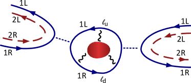
Figure 1: A gate-defined quantum dot (QD) operating in the quantum Hall regime (filling factor $\nu=2$). The QD consists of two parts. The outer channels (denoted by 1R and 1L, blue solid lines) form a ring shaped region. Tunneling between this region and the associated channels outside the QD is denoted by dotted blue lines. The inner channels (denoted by 2R and 2L, red dashed lines) define an isolated puddle (or state) tunnel-coupled to leads (the coupling is not shown in the figure). Wiggly lines represent the electrostatic interaction between the localized puddle and the outer edge mode of the QD. The parameter $\ell_{\mathrm{u}}$ ($\ell_{\mathrm{d}}$) denotes the length of the upper (lower) arm of the outer channel in the QD. The transmission amplitude of electrons traveling along channel 1R towards the dot is measured by embedding it in one arm of a Mach-Zehnder interferometer (not shown).

Two gate controlled constrictions in the Hall bar form a QD (cf. Fig. 1). In the QH regime with $\nu=2$ the electrons move inside the QD along two chiral edge modes. We focus on the transmission of the outer channel. Assuming that the magnitude of charge fluctuations on the inner mode (the localized puddle in Fig. 1) do not exceed an electron charge, it is reasonable to treat it as a localized level which may be either occupied or empty. The spatial structure of the outer edge channel of the QD is important, and in what follows will be taken into account. The gates at the left and right sides of the dot control the corresponding tunneling amplitudes. Tunneling between the two edge channels is suppressed as these correspond to oppositely spin polarized modes. The respective couplings of the outer channel and the inner puddle to the external edge modes define two time scales, namely the typical times for charge fluctuations in the corresponding region. It will be assumed that during the passage of one electron through the outer region, the localized level’s occupation remains unchanged, i.e. each passing electron through the outer region senses the localized level as a non-dynamical environment Stern et al. (1990).

Our aim is to calculate the transmission amplitude through the QD. We first consider the zero temperature quantum regime, and later will generalize our discussion to finite temperatures. The effect of the localized level is to provide an electron passing through the outer region of the QD with an extra phase, if this level is occupied Rosenow and Gefen (2012). Specifically, an electron occupying the localized level induces a change in the density of electrons at channels 1R and 1L. Employing the Thomas-Fermi approximation, this change is $\delta\rho_{\mathrm{R/L}}(x)=-eV_{\mathrm{R}/\mathrm{L}}(x)/{2\pi\hbar v}$, where $V_{\mathrm{R}/\mathrm{L}}(x)$ is the potential induced in channel 1R(1L) by the electron occupying the localized level, whose charge is $e<0$; $x$ is the spatial coordinate along the corresponding channel, and $v$ is the velocity of electrons along the channel. When the localized level is empty, an electron at the Fermi level $\varepsilon_{\mathrm{F}}$ acquires a phase $\varepsilon_{\mathrm{F}}\Delta x/\hbar v$ while traversing a distance $\Delta x$. In the presence of the potential $V_{\mathrm{R/L}}(x)$, i.e. when the localized level is occupied, the chemical potential changes locally by $-eV_{\mathrm{R/L}}(x)$. This, in turn, induces an extra phase equal to $-e\int_{0}^{\Delta x}\mathrm{d}x\,V_{\mathrm{R/L}}/\hbar v=2\pi\int_{0}^{\Delta x}\mathrm{d}x\,\delta\rho_{\mathrm{R/L}}(x)\equiv\theta_{\mathrm{R}}(\theta_{\mathrm{L}})$, where $\theta_{\mathrm{R}}+\theta_{\mathrm{L}}=2\pi$. The last equality reflects the fact that the total screening charge is $e$. For symmetric screening between channels 1R and 1L, $\theta_{\mathrm{R}}=\theta_{\mathrm{L}}=\pi$. Similarly, we define the screening phase $\theta$, which denotes the extra phase accumulated by an electron while winding once along channels 1R and 1L inside the QD. It turns out that the results of our calculation can be formulated using only the screening phases $\theta$ and $\theta_{\mathrm{R}}$.

The spatial dependence of $\delta\rho_{\mathrm{R/L}}(x)$ and the ensuing screening phase is important for the analysis of the transmission amplitude. We note that part or all of the screening takes place inside the QD. Then multiple winding trajectories imply multiple accumulation of the screening phase $\theta$. Clearly, $0\leq\theta\leq 2\pi$, where $\theta/2\pi$ is the fraction of electron charge screened inside the QD. Similarly, $0\leq\theta_{\mathrm{R}}\leq 2\pi$, where $\theta_{\mathrm{R}}/2\pi$ is the fraction of electron charge screened along channel 1R. Below we assume that screening does not take place along channels 2R and 2L (generalization beyond this assumption is straightforward).

In order to measure the transmission amplitude through the QD, the latter is embedded in one arm of a MZI (“upper”). The wave packet of an electron injected into the MZI is split into two upon arriving at its first junction. The lower partial wave, $\left|\mathrm{d}\right\rangle$, goes directly towards the second junction and interferes with the part of the upper partial wave that is transmitted through the QD, $\left|\mathrm{u}\right\rangle$. The current through the MZI as measured at one of its drains is proportional to the probability of an electron to arrive at that drain. Thus, the current is a function of the transmission phase through the QD.

The scattering matrix of the QD depends on the initial state of the isolated subsystem consisting of the localized level and the tunnel-coupled lead(s) (red dashed lines and puddle in Fig. 1). Formally, this state is a Slater determinant built of the eigenstates of that subsystem. Here, we do not include the interaction between the localized state and the outer edge mode of the QD since it does not change our picture in a qualitative manner. However, it is possible to show  that this subsystem can be treated as a two-state system, whose wave function is $\sqrt{1-n}\left|0\right\rangle+\sqrt{n}\left|1\right\rangle$. Here $\left|\sigma\right\rangle$ is a basis state vector corresponding to an empty ($\sigma=0$) or occupied ($\sigma=1$) localized level; an unimportant relative phase factor is omitted. Due to the fermionic statistics of the electrons, the probability of the localized level to be occupied, $n$, equals its mean occupation. The calculation of $n$ is elementary , Mahan (2000). The result is

$$n=\frac{1}{\pi}\left[\arctan\left(\frac{\mu-\epsilon_{0}}{\Gamma}\right)+\frac{\pi}{2}\right]\,,$$ (1)

where $\mu$ is the chemical potential of the system, $\epsilon_{0}$ the eigenenergy of the localized state, and $\Gamma$ its width due to the tunnel-coupled leads.

We calculate  the transmission amplitude through the QD employing scattering matrices and taking into account properly the extra phases $\theta$ and $\theta_{\mathrm{R}}$. If the localized level is occupied, the transmission amplitude through the QD for an electron traveling along the channel 1R is

$$t_{\mathrm{QD}}(\epsilon,\theta,\theta_{\mathrm{R}})=\frac{\gamma e^{i(\epsilon\ell_{\mathrm{d}}/\ell+\theta_{\mathrm{R}})}}{1-e^{i(\epsilon-\theta)}+\gamma}\,.$$ (2)

Here $\ell=\ell_{\mathrm{d}}+\ell_{\mathrm{u}}$ is the circumference of the outer channel inside the QD, which is the sum of the lower ($\ell_{\mathrm{d}}$) and upper ($\ell_{\mathrm{u}}$) lengths (see Fig. 1). The dimensionless parameter $\epsilon\equiv 2\pi\alpha V_{g}/\Delta$ , shifting the outer region energy levels, is proportional to the gate voltage $V_{g}$ with lever arm $\alpha>0$. $\Delta=2\pi\hbar v/\ell$ is the level spacing in the bare outer region, namely in the absence of the inner puddle. The dimensionless parameter $\gamma$ reflects the width of the levels of the outer part of the QD in the absence of the inner puddle. The phase $\theta_{\mathrm{R}}$ accounts for the fact that part of the screening takes place on channel 1R outside the QD. The ensuing phase of the expression in (2) is the added contributions accumulated inside and outside the QD. In a generic case (beside the cases $\ell_{\mathrm{d}}/\ell=0,1$ which are unfeasible), and in a situation where the phases $\theta$ and $\theta_{\mathrm{R}}$ do not vary with energy, the transmission amplitude described by Eq. (2) does not have phase lapses.

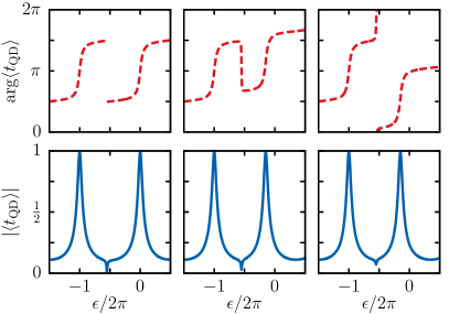
Figure 2: Transmission phase through the QD (red dashed lines, top) and magnitude of coherent oscillations in the MZI (blue solid lines, bottom) in the strong coupling regime for the sequence $(N_{\mathrm{o}},N_{\mathrm{i}})\rightarrow(N_{\mathrm{o}}+1,N_{\mathrm{i}})\rightarrow(N_{\mathrm{o}},N_{\mathrm{i}}+1)\rightarrow(N_{\mathrm{o}}+1,N_{\mathrm{i}}+1)$ as a function of the dimensionless energy parameter $\epsilon$ for symmetric ($\theta_{\mathrm{R}}=\pi$, left) and slightly asymmetric ($\theta_{\mathrm{R}}=1.3\pi$ (center) and $\theta_{\mathrm{R}}=0.7\pi$ (right)) setups. The left (center, right) plot depicts a sharp (smeared) phase lapse accompanied by a full (partial) suppression of the coherent oscillations through the MZI. The energy level of the outer region and the occupancy of the inner region (cf. Eq. (1)) are controlled by a common gate voltage $V_{g}$ with lever arms $\alpha$ and $\beta$ through the relations $\epsilon=2\pi\alpha V_{g}/\Delta$ and $(\mu-\epsilon_{0})/\Gamma=(\beta V_{g}+c)/\Gamma$, respectively, where $\Delta$ is the level spacing in the outer region, $\Gamma$ is the level width in the inner region, $(\beta/\alpha)\cdot(\Delta/2\pi\Gamma)=20$ and $c/\Gamma=22\pi$. Here, using dimensionless parameters, the level spacing of the outer edge (in the absence of the inner edge) is $2\pi$. We consider the symmetric case $\ell_{\mathrm{d}}/\ell=1/2$, and weak coupling to the leads, $\gamma=1/4$. The screening phase $\theta=2\pi$ (left) or $\theta=1.7\pi$ (center and right) imply full and almost full screening inside the QD, respectively.

The transmission probability through the MZI is obtained by employing a pure state density matrix . This yields

$$T=\mathrm{Tr}\left(\hat{\rho}\hat{D}\right)=\frac{1}{4}+\frac{1}{4}\left[(1-n)\left|t_{\mathrm{QD}}(0)\right|^{2}+n\left|t_{\mathrm{QD}}(1)\right|^{2}\right]\\ +\frac{1}{2}\Re\left[e^{-i\phi}\left[(1-n)t_{\mathrm{QD}}(0)+nt_{\mathrm{QD}}(1)\right]\right]\\ =\frac{1}{4}+\frac{1}{4}\left\langle\left|t_{\mathrm{QD}}\right|^{2}\right\rangle+\frac{1}{2}\Re\left[e^{-i\phi}\left\langle t_{\mathrm{QD}}\right\rangle\right]\,.$$ (3)

Here $\hat{\rho}$ is a density matrix constructed from the wave function of the whole system. It corresponds to the interfering electron being either scattered by the QD or transmitted through the lower MZI arm. The operator $\hat{D}$ is defined by $\left(\left\langle\sigma\right|\otimes\left\langle s\right|\right)\hat{D}\left(\left|s^{\prime}\right\rangle\otimes\left|\sigma^{\prime}\right\rangle\right)=\delta_{\sigma\sigma^{\prime}}/2$ for all combinations of $s,s^{\prime}=\mathrm{u},\mathrm{d}$. The operator $\hat{D}$ has two functionalities, namely it selects only the part of the wave function that arrives at the measured drain, and taking the trace over $\hat{D}$ integrates out the environmental degrees of freedom . The phase $\phi=2\pi\Phi/\Phi_{0}$, where $\Phi$ is the magnetic flux enclosed by the MZI arms, $\Phi_{0}=2\pi\hbar c/|e|$ the magnetic flux quantum, $e$ the charge of an electron and $c$ the speed of light. The transmission amplitudes $t_{\mathrm{QD}}(1)$ and $t_{\mathrm{QD}}(0)$ are abbreviations for $t_{\mathrm{QD}}(\epsilon,\theta,\theta_{\mathrm{R}})$ and $t_{\mathrm{QD}}(\epsilon,0,0)$, respectively (cf. Eq. (2)). It should be emphasized that our calculation is valid in the regime where the time interval between two consecutive transmitted electrons is sufficient for the inner puddle to relax to its ground state. In the third line of Eq. (3) and henceforth angular brackets $\langle\ldots\rangle$ denote the average value of the quantity inside the brackets, calculated with respect to the probability distribution function

$$P(\tilde{\theta},\tilde{\theta}_{\mathrm{R}})=\begin{cases}n&\mathrm{for\;the\;phases\;to\;be\;(\theta,\theta_{\mathrm{R}})}\,,\\ 1-n&\mathrm{for\;the\;phases\;to\;be\;(0,0)}\,.\end{cases}$$ (4)

The parameters $\theta$ and $\theta_{\mathrm{R}}$ are defined above, and corresponding random variables are denoted by $\tilde{\theta}$ and $\tilde{\theta}_{\mathrm{R}}$. Thus the last equality in Eq. (3) shows that the presence of the localized state turns the transmission amplitude of the QD into a random quantity, whose probability distribution function is determined by $n$ (cf. Ref Stern et al. (1990)).

The two quantities of interest are the transmission phase through the QD, $\arg\left\langle t_{\mathrm{QD}}\right\rangle$, and the magnitude of the coherent oscillations of the current through the MZI, $\left|\left\langle t_{\mathrm{QD}}\right\rangle\right|$. From Eq. (3) we find

$$\arg\left\langle t_{\mathrm{QD}}\right\rangle =\arg\left[t_{\mathrm{QD}}(\epsilon,0,0)\left\langle\zeta\right\rangle\right]\,,$$ (5a)

$$\left|\left\langle t_{\mathrm{QD}}\right\rangle\right| =\left|t_{\mathrm{QD}}(\epsilon,0,0)\right|\left|\left\langle\zeta\right\rangle\right|\,,$$ (5b)

where

$$\zeta(\epsilon,\tilde{\theta},\tilde{\theta}_{\mathrm{R}})=\frac{1+\gamma-e^{i\epsilon}}{1+\gamma-e^{i(\epsilon-\tilde{\theta})}}e^{i\tilde{\theta}_{\mathrm{R}}}\,.$$ (6)

Here averages are calculated with respect to the probability distribution (4), e.g.

$$\left\langle\zeta\right\rangle=1-n+n\zeta(\epsilon,\theta,\theta_{\mathrm{R}})\,.$$ (7)

Clearly, the presence of the inner puddle induces a change in the transmission phase such that $\arg\left[t_{\mathrm{QD}}(\epsilon,0,0)\right]\rightarrow\arg\left[t_{\mathrm{QD}}(\epsilon,0,0)\left\langle\zeta\right\rangle\right]$. The resulting phase is the sum of the transmission phase through the “bare” outer region and $\arg(\left\langle\zeta\right\rangle)$. Phase lapses can occur only due to the phase evolution of $\left\langle\zeta\right\rangle$, since $\arg\left[t_{\mathrm{QD}}(\epsilon,0,0)\right]$ by itself evolves continuously. Moreover, it is evident that any interesting physics that may be hidden in $\left\langle\zeta\right\rangle$ will generically be more pronounced if it happens to occur in between resonances of the “bare” outer region — there the phase of $t_{\mathrm{QD}}(\epsilon,0,0)$ is practically constant.

A phase lapse occurs if $\left\langle\zeta\right\rangle$ vanishes at a certain $V_{g}$. Eq. (5b) shows that this abrupt jump in the phase is accompanied by complete suppression of the coherent oscillations in the MZI. Solution of the complex equation $\left\langle\zeta\right\rangle=0$ requires both $(1-n)/n=\left|\zeta\left(\epsilon,\theta,\theta_{\mathrm{R}}\right)\right|$ and fine tuning of the phases $\theta$ and $\theta_{\mathrm{R}}$ such that $\arg\left[\zeta\left(\epsilon,\theta,\theta_{\mathrm{R}}\right)\right]=\pi$. These phases are determined by the geometry of the setup (the location of the localized level, the symmetry of the QD, etc …), which fixes the way screening is divided in the system. The geometry can be controlled by tuning the gates that define the QD. Fig. 2 depicts the emergence of phase lapses in the transmission amplitude through the QD and the accompanying dephasing of the MZI.

This very general picture outlined above can be put to work employing parameters that reflect the sample’s specific electrostatic features. These parameters determine the effect of the gate voltage on the inner and outer parts of the QD, and hence the evolution of the transmission phase. Specifically, we employ a charging energy model , which leads to a stability diagram of the charge distribution between the inner and outer parts of the QD, with charges $N_{\mathrm{i}}$ and $N_{\mathrm{o}}$, respectively.

In order to extract a physical picture out of this many-parameter problem, we focus on two important limits, namely that of a strong (“S”) and a weak (“W”) coupling between the two parts of the QD. We examine each of these limits in view of two interesting scenarios that may occur vis-à-vis the change in occupancy of the two parts of the dot as a common gate voltage is varied . These scenarios are (a) $(N_{\mathrm{o}},N_{\mathrm{i}})\rightarrow(N_{\mathrm{o}},N_{\mathrm{i}}+1)$, and (b) $(N_{\mathrm{o}},N_{\mathrm{i}})\rightarrow(N_{\mathrm{o}}-1,N_{\mathrm{i}}+1)$.

We begin with the strong interaction case (S), which implies $\theta\simeq 2\pi$. In S(a) the outer part is positioned in a valley between resonances, while the inner part is tuned to be near a resonance peak and eventually crosses this peak as a function of gate voltage. Under these conditions a phase lapse occurs if $\theta_{\mathrm{R}}\simeq 0,2\pi$ . In S(b) there is a population switching (see e.g. Baer et al. (2013)). This means that both parts of the QD change their occupation by $\pm 1$. If $\theta_{\mathrm{R}}\simeq\pi$, as appears to be achieved quite naturally in experiments Weisz et al. (2012), then this scenario leads to a phase lapse .

We turn now to the weak coupling regime, where $\theta\simeq 0$. Scenario W(a) may occur when the outer channel is not too close to a resonance, so that its occupation is not affected by a change in the occupation of the inner puddle. Then there is no discontinuity (yet possibly a sharp signature) in the transmission phase. Scenario W(b), which implies a population switching, can occur only if the outer channel is close to a resonance. Then (in a generic case) a phase lapse occurs if $\theta_{\mathrm{R}}\simeq 0,2\pi$, where $\theta_{\mathrm{R}}\simeq 0$ is more likely in a weak coupling scenario.

Finite temperatures — Our analysis so far pertains to the strictly zero temperature limit. Two modifications need to be introduced at finite temperatures: (i) The initial state of the subsystem composed of the localized level and the tunnel-coupled lead(s) must be described by a mixed density matrix (rather than a wave function). This is easily handled as the operator $\hat{D}$ is diagonal in the localized level coordinate $\sigma$. This implies that only the corresponding diagonal elements of $\hat{\rho}$ are of importance for the calculation of the transmission probability through the MZI. (ii) The electronic beam traveling along the arms of the MZI has finite width in energy. This means that the entire interference pattern is a juxtaposition of many monochromatic partial beams; each such partial beam travels both in the upper and lower arm of the MZI. Summing over all contributions will naturally lead to thermal smearing and reduction of the interference signal. This, however, is not our main focus here. We note that in scenario S(b) above, each such partial interference would be shifted by a phase $\pi$ due to the entry/exit of an electron to the localized level, and will be consequently fully dephased. That would mean that abrupt phase lapse accompanied by full dephasing will take place at finite temperature as well. This phase lapse and dephasing will take place on the background of an interference contrast which decreases with temperature. We note that the physics is less simple with the other scenarios outlined above. Charge fluctuations on the localized level will affect electron trajectories with different winding numbers differently. That would imply, in turn, that the efficiency of dephasing will vary with energy, leading to temperature dependent smearing of the phase lapses.

To conclude, we have studied the transmission amplitude through a QD operating in the QH regime and have found that it displays phase lapses due to interactions between different spin populations inside the dot. Specifically, phase lapses occur in the presence of quantum or thermal fluctuations, and are related to full dephasing of the electrons. We have developed a formalism which allows to take into account the influence of both types of fluctuations in a unified way, and have identified the experimentally relevant regime of a strongly interacting and spatially symmetric setup, where phase lapses are expected to occur due to population switching in the valley between transmission resonances. These phase lapses are not thermally broadened, in contrast to the zero magnetic field case.

We are grateful to E. Weisz and M. Heiblum for useful discussions, and to I. Chernii, I. Levkivskyi, and E. Sukhorukov for discussing with us their unpublished work. Financial support by the German-Israel Foundation (GIF), the Minerva Foundation, the Israel Science Foundation, and the Federal Ministry of Education and Research (BMBF) is acknowledged.

Supplemental Material

Transmission amplitude through the QD

We calculate the transmission amplitude through the QD employing scattering matrices and taking into account properly the extra screening phases $\theta$ and $\theta_{\mathrm{R}}$. If the localized level is occupied, the transmission amplitude through the QD of an electron traveling along channel 1R is

$$t_{\mathrm{QD}}(\epsilon,\theta,\theta_{\mathrm{R}})=\frac{t_{\mathrm{A}}t_{\mathrm{B}}e^{i(\epsilon\ell_{\mathrm{d}}/\ell+\theta_{\mathrm{R}})}}{1-r_{\mathrm{B}}r_{\mathrm{A}}^{\prime}e^{i(\epsilon-\theta)}}\,.$$ (I.1)

Here $\ell=\ell_{\mathrm{d}}+\ell_{\mathrm{u}}$ is the circumference of the outer channel of the QD, which is the sum of the lower ($\ell_{\mathrm{d}}$) and upper ($\ell_{\mathrm{u}}$) lengths (see Fig. 1 in the main text). The dimensionless parameter $\epsilon\equiv\mu\ell/\hbar v$, where $\mu$ is the chemical potential of the system, and $v$ is the velocity of the electrons. To mimic the effect of a gate voltage $V_{g}$, capable of shifting the outer region energy levels, we take $\epsilon=2\pi\alpha V_{g}/\Delta$ with $\alpha>0$ .The parameters $t_{\mathrm{A}}$, $t_{\mathrm{B}}$, $r_{\mathrm{A}}^{\prime}$ and $r_{\mathrm{B}}$ are elements of the scattering matrices associated with the left (A) and right (B) tunneling bridges that define the QD; here $t$ ($r$) refers to a transmission (reflection) amplitude of an electron propagating from left to right, and a prime denotes the opposite direction. For example, $r_{\mathrm{B}}$ is the reflection amplitude of an electron, traveling along channel 1R inside the QD and impinging on the right junction from the left, to be reflected back to channel 1L inside the QD (Fig. 1 in the main text).

The level width associated with the outer part of the QD in the absence of the inner puddle can be identified by expanding (I.1) near a resonance, and singling out the quantity that plays the role of the Lorentzian width. Assuming $r_{\mathrm{B}}r^{\prime}_{\mathrm{A}}$ to be real, resonance transmission occurs at integral multiples of $\epsilon=2\pi$. Expansion around $\epsilon=0$ gives $\gamma=\left(1-r^{\prime}_{\mathrm{A}}r_{\mathrm{B}}\right)/r^{\prime}_{\mathrm{A}}r_{\mathrm{B}}$. Assuming that the two tunnel-bridges that define the QD have equal transmission and reflection probabilities, and substituting the foregoing expression in (I.1), one obtains Eq. (2) of the main text up to an unimportant constant phase factor.

Initial wave function of a localized level tunnel-coupled to lead

At zero temperature the isolated subsystem composed of the localized state and the tunnel-coupled lead is a many-body system, whose wave function can be written as a linear combination of Slater determinants in the basis states $\left\{\sigma;n_{k_{1}},n_{k_{2}},\ldots,n_{k_{N}}\right\}\equiv\left\{\sigma;\xi\right\}$. Here $\sigma=0,1$ denotes an empty or occupied localized state and $n_{k_{i}}$ is the occupation of the state $k_{i}$ in the lead (the lead accommodates $N$ single-particle states). Formally,

$$\left|\mathrm{GS}\right\rangle=\sum_{\sigma;\xi}c_{\sigma;\xi}\left|\left\{\sigma;\xi\right\}\right\rangle\\ =\sum_{\xi}c_{0;\xi}\left|\left\{\sigma=0;\xi\right\}\right\rangle+\sum_{\xi}c_{1;\xi}\left|\left\{\sigma=1;\xi\right\}\right\rangle\\ =\left|\sigma=0\right\rangle\otimes\left|\mathrm{FS},0\right\rangle+\left|\sigma=1\right\rangle\otimes\left|\mathrm{FS},1\right\rangle\,.$$ (I.2)

Here $\left|\left\{\sigma;\xi\right\}\right\rangle$ is a Slater determinant built from the corresponding occupied states and $c_{\sigma;\xi}$ is the associated amplitude. The ket $\left|\mathrm{FS},0\right\rangle\equiv\sum_{\xi}c_{0;\xi}\left|\left\{0;\xi\right\}\right\rangle$ physically denotes the Fermi sea when the localized state is empty and similarly for $\left|\mathrm{FS},1\right\rangle$.

Thus, it is found that the environment can be treated as a two-state system with $\left|0\right\rangle\equiv\left|\sigma=0\right\rangle\otimes\left|\mathrm{FS},0\right\rangle$ and $\left|1\right\rangle\equiv\left|\sigma=1\right\rangle\otimes\left|\mathrm{FS},1\right\rangle$.

Mean occupation of localized level

The mean occupation of the localized state can be calculated as follows. The retarded Green’s function of the localized level, which is coupled to outer leads, is $G^{\mathrm{R}}(E)=(E-\epsilon_{0}+i\Gamma)^{-1}$. Here $\epsilon_{0}$ is the level’s eigenenergy and $\Gamma$ is the level’s width. This yields a spectral density $B(E)=-2\Im\mathrm{Tr}G^{\mathrm{R}}(E)=2\Gamma/[(E-\epsilon_{0})^{2}+\Gamma^{2}]$. The mean occupation is then given by

$$n=\int_{-\infty}^{\infty}\frac{\mathrm{d}E}{2\pi}\frac{1}{e^{(E-\mu)/T}+1}\frac{2\Gamma}{(E-\epsilon_{0})^{2}+\Gamma^{2}}\,.$$ (I.3)

Calculation of the integral in the limit of $T\gg\Gamma$ gives that the mean occupation equals the Fermi-Dirac function, $n=[e^{(\epsilon_{0}-\mu)/T}+1]^{-1}$. In the opposite limit of zero temperature the Fermi-Dirac function in the integrand of Eq. (I.3) is the step function $\Xi(\mu-E)$, where $\Xi(x)=1$ ($x>0$) or $\Xi(x)=0$ ($x<0$). Eq. (I.3) then gives

$$n=\frac{1}{\pi}\left[\arctan\left(\frac{\mu-\epsilon_{0}}{\Gamma}\right)+\frac{\pi}{2}\right]\,.$$ (I.4)

The density matrix of the composite system

We are interested in the wave function of the whole system that corresponds to the interfering electron being either scattered by the QD or transmitted through the lower Mach-Zehnder interferometer (MZI) arm. This wave function can be written as

$$\left|\psi\right\rangle=\left|\psi_{\mathrm{u}}\right\rangle+\left|\psi_{\mathrm{d}}\right\rangle$$ (I.5)

with

$$\left|\psi_{\mathrm{u}}\right\rangle = \frac{1}{\sqrt{2}}\left[t_{\mathrm{QD}}(1)\left|\mathrm{u}\right\rangle\otimes\sqrt{n}\left|1\right\rangle+t_{\mathrm{QD}}(0)\left|\mathrm{u}\right\rangle\otimes\sqrt{1-n}\left|0\right\rangle\right.$$

$$\left.+r_{\mathrm{QD}}(1)\left|\mathrm{w}\right\rangle\otimes\sqrt{n}\left|1\right\rangle+r_{\mathrm{QD}}(0)\left|\mathrm{w}\right\rangle\otimes\sqrt{1-n}\left|0\right\rangle\right]\,,$$

$$\left|\psi_{\mathrm{d}}\right\rangle = \frac{1}{\sqrt{2}}e^{i\phi}\left|\mathrm{d}\right\rangle\otimes\left(\sqrt{1-n}\left|0\right\rangle+\sqrt{n}\left|1\right\rangle\right)\,.$$ (I.6)

Here $\left|\mathrm{d}\right\rangle$ is the lower partial wave that goes directly towards the second junction, and interferes with the part of the upper partial wave that is transmitted through the QD, $\left|\mathrm{u}\right\rangle$. The other part of the upper partial wave, namely the one which is reflected from the QD to another drain, is denoted by $\left|\mathrm{w}\right\rangle$. The phase $\phi$ is defined in the main text after Eq. (3). The transmission amplitudes $t_{\mathrm{QD}}(1)$ and $t_{\mathrm{QD}}(0)$ are abbreviations for $t_{\mathrm{QD}}(\epsilon,\theta,\theta_{\mathrm{R}})$ and $t_{\mathrm{QD}}(\epsilon,0,0)$, respectively (cf. Eq. (2) in the main text). The reflection amplitudes $r_{\mathrm{QD}}(1)$ and $r_{\mathrm{QD}}(0)$ are similarly defined.

The density matrix used in Eq. (3) of the main text is then $\hat{\rho}=\left|\psi\right\rangle\left\langle\psi\right|$.

The projection operator $\hat{D}$

The operator $\hat{D}$ is essentially a projection operator, which selects only the part of the wave function that arrives at one drain of the MZI. It can be obtained as follows. The two junctions of the MZI define three regions, each of which consists of two segments that accommodate the propagation of a partial wave. Formally, the state of an electron in the region after the second junction can be represented by a two-component wave function with basis vectors $|\mathrm{u^{\prime}}\rangle$ and $|\mathrm{d^{\prime}}\rangle$, corresponding to a propagation towards the upper or lower drain, respectively. In this basis the operator $\hat{D}^{\prime}=|\mathrm{u^{\prime}}\rangle\langle\mathrm{u^{\prime}}|$, assuming the upper drain is the one which is measured in the experiment. In the main text, though, we use the basis vectors $|\mathrm{u}\rangle$ and $|\mathrm{d}\rangle$, which correspond to the two segments of the MZI in the regions just in front of the second junction. Hence we need to perform the transformation $\hat{D}=\hat{S}^{\dagger}\hat{D}^{\prime}\hat{S}$, where $\hat{S}$ is the scattering matrix of the second junction. A valid scattering matrix describing a symmetric junction is

$$\hat{S}=\frac{1}{\sqrt{2}}\left(\begin{array}[]{cc}\phantom{-}1&1\\ -1&1\end{array}\right)\,.$$ (I.7)

Using that matrix one obtains that $\hat{D}$ is a $2\times 2$ matrix with all entries equal to $1/2$. Since neither the arrival to the drain nor the passage through the second junction alters the state of the localized level, one arrives at the definition $\left(\left\langle\sigma\right|\otimes\left\langle s\right|\right)\hat{D}\left(\left|s^{\prime}\right\rangle\otimes\left|\sigma^{\prime}\right\rangle\right)=\delta_{\sigma\sigma^{\prime}}/2$ for all combinations of $s,s^{\prime}=\mathrm{u},\mathrm{d}$.

Charge stability diagram and scenarios for changes of occupancy

We model the outer and inner parts of the QD by conductors, and write the total energy of the QD as

$$E=\frac{K_{\mathrm{o}}}{2}\left(N_{\mathrm{o}}-\frac{\epsilon}{2\pi}-\varphi\right)^{2}+\frac{K_{\mathrm{i}}}{2}\left(N_{\mathrm{i}}-\frac{\beta}{\alpha}\frac{\Delta}{\Delta_{\mathrm{i}}}\frac{\epsilon}{2\pi}+\varphi\right)^{2}\\ +K_{\mathrm{oi}}\left(N_{\mathrm{o}}-\frac{\epsilon}{2\pi}-\varphi\right)\left(N_{\mathrm{i}}-\frac{\beta}{\alpha}\frac{\Delta}{\Delta_{\mathrm{i}}}\frac{\epsilon}{2\pi}+\varphi\right)\,.$$ (I.8)

Here $K_{\mathrm{o}}$, $K_{\mathrm{i}}$ and $K_{\mathrm{oi}}$ are positive and can be related to the conductors capacitance matrix. The number of flux quanta penetrating the QD is $\varphi$. The charges in the outer and inner regions, $N_{\mathrm{o}}$ and $N_{\mathrm{i}}$, respectively, are taken to be integers. They are determined by the requirement that the energy function be minimal for given values of all the other parameters. The parameters $\Delta$ and $\Delta_{\mathrm{i}}$ are the level spacing of the outer and inner regions, respectively (the former is defined in the main text). The parameter $\epsilon$ is the dimensionless gate voltage appearing in the main text and is related to the gate voltage $V_{g}$. It enters the energy function in such a way that — in the absence of interactions between the inner and the outer regions — $N_{\mathrm{o}}$ ($N_{\mathrm{i}}$) increases by one when $\alpha V_{g}$ ($\beta V_{g}$) increases by $\Delta$ ($\Delta_{\mathrm{i}}$). Figs. I.1 and I.2 show examples of stability diagrams.

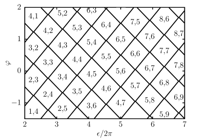
Figure I.1: Example of a stability diagram describing the charge distribution in the QD in the weak coupling regime. The pair of numbers in each polygon denotes the equilibrium occupation of the outer and inner regions, $N_{\mathrm{o}},N_{\mathrm{i}}$. Here we set $K_{\mathrm{o}}=1$, $K_{\mathrm{i}}=1.5$, $K_{\mathrm{oi}}=0.02$ and $(\beta/\alpha)\cdot(\Delta/\Delta_{\mathrm{i}})=1.2$.

As $V_{g}$ is swept, several scenarios (charge variations) may occur. The possible scenarios and their probabilities can be inferred from the stability diagram. This is simply the relative length of the appropriate polygon edge projected on the $\varphi$-axis. Note that only 3 independent parameters determine the probability of the scenarios; they can be chosen as $K_{\mathrm{o}}/K_{\mathrm{oi}}$, $K_{\mathrm{i}}/K_{\mathrm{oi}}$ and $(\beta/\alpha)\cdot(\Delta/\Delta_{\mathrm{i}})$.

The relation between the energy function and the transmission phase is established in the following way. We first show that the screening is given by $\theta=2\pi K_{\mathrm{oi}}/K_{\mathrm{o}}$. This can be obtained by treating $N_{\mathrm{o}}$ and $N_{\mathrm{i}}$ as continuous variables for a moment, and requiring that $\partial E/\partial N_{\mathrm{o}}=0$. One then obtains that, if $N_{\mathrm{i}}$ increases by 1, then $N_{\mathrm{o}}$ varies by $-K_{\mathrm{oi}}/K_{\mathrm{o}}$. In accordance with Eq. (2) of the main text we identify that $\theta=2\pi K_{\mathrm{oi}}/K_{\mathrm{o}}$. The parameter $c$ in the main text is chosen so as to fit the investigated scenario. For instance, to investigate population switching we tune $c$ such that the inner puddle has mean occupation $1/2$ when the outer region is in a valley and $\theta$ is sufficiently large to shift the outer region beyond a peak.

The specific values of the parameters appearing in (I.8) determine the stability diagram of the QD. These are sample-dependent, and can be estimated for a given experimental realization. To exemplify the type of analysis one may perform, and to gain some insight into the physics, we concentrate on two extreme regimes, namely the regime where the interaction between the inner and outer regions of the QD is weak (“W”), and the regime where the interaction is strong (“S”). For concreteness, we take $(\beta/\alpha)\cdot(\Delta/\Delta_{\mathrm{i}})=1.2$. Moreover, we assume that the inner puddle has a slightly higher charging energy than the outer region, and put $K_{\mathrm{o}}=1$ and $K_{\mathrm{i}}=1.5$.

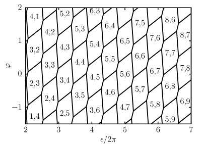
Figure I.2: Example of a stability diagram describing the charge distribution in the QD in the strong coupling regime. Here we set $K_{\mathrm{o}}=1$, $K_{\mathrm{i}}=1.5$, $K_{\mathrm{oi}}=0.85$ and $(\beta/\alpha)\cdot(\Delta/\Delta_{\mathrm{i}})=1.2$.

Weak coupling regime — Taking $K_{\mathrm{oi}}=0.02$, which implies $\theta=0.04\pi$, yields that the probable scenarios are $(N_{\mathrm{o}},N_{\mathrm{i}})\rightarrow(N_{\mathrm{o}},N_{\mathrm{i}}+1)$ (W(a)) and $(N_{\mathrm{o}},N_{\mathrm{i}})\rightarrow(N_{\mathrm{o}}+1,N_{\mathrm{i}})$; population switching $(N_{\mathrm{o}},N_{\mathrm{i}})\rightarrow(N_{\mathrm{o}}-1,N_{\mathrm{i}}+1)$ (W(b)) is rare (cf. Fig. I.1). In W(a) the outer region is not too close to a resonance, and $\zeta\simeq e^{i\theta_{\mathrm{R}}}$. Since $\theta$ is small, presumably also $\theta_{\mathrm{R}}\simeq 0$, namely the screening takes place somewhere else — neither in the outer region of the dot nor in the upper MZI arm. Then one may observe a sharp signature in the transmission phase, but not a discontinuity. We analyse W(b) by writing $\theta=m\gamma$ and $\epsilon=p\gamma$ where $m$ and $p$ are positive parameters that fulfill $m>p$. Expansion of $\zeta$ around small values of $m\gamma$ and $p\gamma$ yields $\zeta\simeq\left(1-ip\right)e^{i\theta_{\mathrm{R}}}/\left(1-ip+im\right)$. Then for $m>p+1/p$ a phase lapse occurs if $\theta_{\mathrm{R}}=-\arctan\left[m/\left[p\left(m-p\right)-1\right]\right]$. In a generic case where $m\ll p(m-p)-1$ a phase lapse occurs if $\theta_{\mathrm{R}}\simeq 0,2\pi$.

Strong coupling regime — Taking $K_{\mathrm{oi}}=0.85$, which implies $\theta=1.7\pi$, yields that the probable scenarios are $(N_{\mathrm{o}},N_{\mathrm{i}})\rightarrow(N_{\mathrm{o}}+1,N_{\mathrm{i}})$, the scenario $(N_{\mathrm{o}},N_{\mathrm{i}})\rightarrow(N_{\mathrm{o}},N_{\mathrm{i}}+1)$ (S(a)) and the scenario $(N_{\mathrm{o}},N_{\mathrm{i}})\rightarrow(N_{\mathrm{o}}-1,N_{\mathrm{i}}+1)$ (S(b)) (cf. Fig. I.2). We analyse S(a) by writing $\theta=2\pi-m\gamma$ and $\epsilon=2\pi-p\gamma$ where $m$ and $p$ are positive parameters that fulfill $m>p$. Expansion of $\zeta$ around small values of $m\gamma$ and $p\gamma$ yields $\zeta\simeq\left(1+ip\right)e^{i\theta_{\mathrm{R}}}/\left(1+ip-im\right)$. Then for $m>p+1/p$ a phase lapse occurs if $\theta_{\mathrm{R}}=\arctan\left\{m/\left[p\left(m-p\right)-1\right]\right\}$. In a generic case where $m\ll p(m-p)-1$ a phase lapse occurs if $\theta_{\mathrm{R}}\simeq 0,2\pi$. In S(b) one has $\zeta\simeq e^{i\theta_{\mathrm{R}}}$, namely $\left\langle\zeta\right\rangle\simeq 1-n+ne^{i\theta_{\mathrm{R}}}$. This gives a phase lapse for $\theta_{\mathrm{R}}\simeq\pi$.

References

- Yacoby et al. (1995) A. Yacoby, M. Heiblum, D. Mahalu, and H. Shtrikman, Phys. Rev. Lett. 74, 4047 (1995).
- Schuster et al. (1997) R. Schuster, E. Buks, M. Heiblum, D. Mahalu, V. Umansky, and H. Shtrikman, Nature (London) 385, 417 (1997).
- Ji et al. (2000) Y. Ji, M. Heiblum, D. Sprinzak, D. Mahalu, and H. Shtrikman, Science 290, 779 (2000).
- Avinun-Kalish et al. (2005) M. Avinun-Kalish, M. Heiblum, O. Zarchin, D. Mahalu, and V. Umansky, Nature (London) 436, 529 (2005).
- Taniguchi and Büttiker (1999) T. Taniguchi and M. Büttiker, Phys. Rev. B 60, 13814 (1999).
- Levy Yeyati and Büttiker (2000) A. Levy Yeyati and M. Büttiker, Phys. Rev. B 62, 7307 (2000).
- Silva et al. (2002) A. Silva, Y. Oreg, and Y. Gefen, Phys. Rev. B 66, 195316 (2002).
- Meden and Marquardt (2006) V. Meden and F. Marquardt, Phys. Rev. Lett. 96, 146801 (2006).
- Golosov and Gefen (2006) D. I. Golosov and Y. Gefen, Phys. Rev. B 74, 205316 (2006).
- Golosov and Gefen (2007) D. I. Golosov and Y. Gefen, New J. Phys. 9, 120 (2007).
- Karrasch et al. (2007) C. Karrasch, T. Hecht, A. Weichselbaum, Y. Oreg, J. v. Delft, and V. Meden, Phys. Rev. Lett. 98, 186802 (2007).
- Goldstein and Berkovits (2007) M. Goldstein and R. Berkovits, New J. Phys. 9, 118 (2007).
- Goldstein et al. (2009) M. Goldstein, R. Berkovits, Y. Gefen, and H. A. Weidenmuller, Phys. Rev. B 79, 125307 (2009).
- Goldstein et al. (2010) M. Goldstein, R. Berkovits, and Y. Gefen, Phys. Rev. Lett. 104, 226805 (2010).
- Hackenbroich et al. (1997) G. Hackenbroich, W. D. Heiss, and H. A. Weidenmüller, Phys. Rev. Lett. 79, 127 (1997).
- Baltin et al. (1999) R. Baltin, Y. Gefen, G. Hackenbroich, and H. Weidenm ller, EPJ B 10, 119 (1999).
- Silvestrov and Imry (2000) P. G. Silvestrov and Y. Imry, Phys. Rev. Lett. 85, 2565 (2000).
- Silvestrov and Imry (2001) P. G. Silvestrov and Y. Imry, Phys. Rev. B 65, 035309 (2001).
- Berkovits et al. (2005) R. Berkovits, F. von Oppen, and Y. Gefen, Phys. Rev. Lett. 94, 076802 (2005).
- König and Gefen (2005) J. König and Y. Gefen, Phys. Rev. B 71, 201308 (2005).
- Sindel et al. (2005) M. Sindel, A. Silva, Y. Oreg, and J. von Delft, Phys. Rev. B 72, 125316 (2005).
- Molina et al. (2012) R. A. Molina, R. A. Jalabert, D. Weinmann, and P. Jacquod, Phys. Rev. Lett. 108, 076803 (2012).
- Molina et al. (2013) R. A. Molina, P. Schmitteckert, D. Weinmann, R. A. Jalabert, and P. Jacquod, Phys. Rev. B 88, 045419 (2013).
- Baltin and Gefen (1999) R. Baltin and Y. Gefen, Phys. Rev. Lett. 83, 5094 (1999).
- Baltin and Gefen (2000) R. Baltin and Y. Gefen, Phys. Rev. B 61, 10247 (2000).
- Note (1) The effect of weak magnetic fields has been noted in Silva et al. (2002) and in Molina et al. (2012); *Molina_2013.
- Halperin (1982) B. I. Halperin, Phys. Rev. B 25, 2185 (1982).
- MacDonald (1990) A. H. MacDonald, Phys. Rev. Lett. 64, 220 (1990).
- Wen (1990) X. G. Wen, Phys. Rev. B 41, 12838 (1990).
- Wen (1991) X. G. Wen, Phys. Rev. B 43, 11025 (1991).
- Prange and Girvin (1990) R. E. Prange and S. M. Girvin, eds., The Quantum Hall Effect, 2nd ed. (Springer-Verlag, New York, 1990).
- Sarma and Pinczuk (1997) S. D. Sarma and A. Pinczuk, eds., Perspectives in Quantum Hall Effects (Wiley, New York, 1997).
- Weisz et al. (2012) E. Weisz, H. K. Choi, M. Heiblum, Y. Gefen, V. Umansky, and D. Mahalu, Phys. Rev. Lett. 109, 250401 (2012).
- Stern et al. (1990) A. Stern, Y. Aharonov, and Y. Imry, Phys. Rev. A 41, 3436 (1990).
- Rosenow and Gefen (2012) B. Rosenow and Y. Gefen, Phys. Rev. Lett. 108, 256805 (2012).
- Note (2) See Supplemental Material for a discussion about the initial wave function of the subsystem consisting of the localized state and the tunnel-coupled lead, the mean occupation , the density matrix , the projection operator , and the charging energy model.
- Mahan (2000) G. D. Mahan, Many-Particle Physics, 3rd ed. (Kluwer Academic / Plenum Publishers, New York, 2000) Chap. 4.2.
- Baer et al. (2013) S. Baer, C. Rössler, T. Ihn, K. Ensslin, C. Reichl, and W. Wegscheider, New Journal of Physics 15, 023035 (2013).