Solar flare-like origin of X-ray flares in gamma-ray burst afterglows

F. Y. Wang^1,2 & Z. G. Dai^1,2

Abstract

X-ray flares detected in nearly half of gamma-ray burst (GRB) afterglows are one of the most intriguing phenomena in high-energy astrophysics[1, 2, 3, 4, 5, 6, 7, 8]. All the observations indicate that the central engines of bursts, after the gamma-ray emission has ended, still have long periods of activity, during which energetic explosions eject relativistic materials, leading to late-time X-ray emission[2, 9, 10]. It is thus expected that X-ray flares provide important clues to the nature of the central engines of GRBs, and more importantly, unveil the physical origin of the flares themselves, which has so far remained mysterious. Here we report statistical results of X-ray flares of GRBs with known redshifts, and show that X-ray flares and solar flares share three statistical properties: power-law energy frequency distributions, power-law duration-time frequency distributions, and power-law waiting time distributions. All of the distributions can be well understood within the physical framework of a magnetic reconnection-driven self-organized criticality system. These statistical similarities, together with the fact that solar flares are triggered by a magnetic reconnection process taking place in the atmosphere of the Sun, suggest that X-ray flares originate from magnetic reconnection-driven events, possibly involved in ultra-strongly magnetized millisecond pulsars[11, 12].

{affiliations}

School of Astronomy and Space Science, Nanjing University, Nanjing 210093, China

Key Laboratory of Modern Astronomy and Astrophysics (Nanjing University), Ministry of Education, Nanjing 210093, China

Gamma-ray bursts (GRBs) are flashes of gamma-rays occurring at the cosmological distances with an isotropic-equivalent energy release from $10^{51}$ to $10^{54}$ ergs[9, 10, 13, 14]. They can be sorted into two classes: short-duration hard-spectrum bursts ( $<2$ s) and long-duration soft-spectrum bursts[15]. Thanks to the rapid-response capability and high sensitivity of the Swift satellite[16], numerous unforeseen features have been discovered, one of which is that about half of bursts have large, late-time X-ray flares with short rise and decay times[4, 5]. The unexpected X-ray flares with an isotropic-equivalent energy from $10^{48}$ to $10^{52}$ ergs have been detected for both long and short bursts[4, 6, 7]. The occurrence times of X-ray flares range from a few seconds to $10^{6}$ seconds after the GRB trigger[8]. Until now, the physical origin of X-ray flares has remained mysterious, although some models have been proposed[9, 10]. Due to 8-year observations of Swift, plentiful of X-ray flare data has been collected. Here we investigate the energy release frequency distribution, duration-time frequency distribution and waiting time distribution of GRB X-ray flares for the first time. On the other hand, it is well known that solar flares with timescale of hours are explosive phenomena in the solar atmosphere with energy release of about $10^{28}-10^{32}$ ergs, which are widely believed to be triggered by a magnetic reconnection process[17]. They have been observed in broadband electromagnetic waves, but we here focus on solar hard X-ray flares.

Although X-ray flares are common phenomena in GRBs and the Sun, the flare energy spans about 20 orders of magnitude and an outstanding question appears, i.e., do GRB X-ray flares and solar flares have a similar physical mechanism? Interestingly, some theoretical models have suggested that GRB X-ray flares could be powered by magnetic reconnection events[11, 12]. However, a physical analogy between GRB X-ray flares and solar flares has not yet been established.

We search for statistical similarities between GRB X-ray flares and solar flares. In particular, we compare statistical properties of the energy release frequency, duration time and waiting time distributions of GRB X-ray flares and solar flares. For X-ray flares of GRBs with known redshifts, we employ the published and archival observed data that allow us to estimate the energy release, duration time and waiting time of each X-ray flare[4, 5, 6, 7, 8]. The total number of flares is 83, including 9 short-burst flares and 74 long-burst flares. The isotropic energy of one flare in the 0.3-10 keV band can be calculated by $E_{\rm iso}=4\pi d^{2}_{L}(z)S_{F}/(1+z)$ , where $S_{F}$ is the fluence, and $d_{L}(z)$ is the luminosity distance calculated for a flat $\Lambda$ CDM universe with $\Omega_{M}=0.3$ , $\Omega_{\Lambda}=0.7$ and $H_{0}=70$ km s^-1 Mpc^-3. The Malmquist bias depending on the luminosity function is poorly known at present. Although GRBs spread over a wide range of redshifts, the Malmquist bias is claimed to be small and negligible[18]. The waiting time in the source’s rest frame can be obtained by $\Delta t=(t_{i+1}-t_{i})/(1+z)$ , where $t_{i+1}$ is the observed starting time of the $i+1$ th flare, $t_{i}$ is the observed starting time of the $i$ th flare, and $1+z$ is the factor to transfer the time into the source-frame one. For the first flare appearing in an afterglow, the waiting time is taken to be $t_{1}/(1+z)$ . We list the measured parameters of 83 X-ray flares in Table S1.

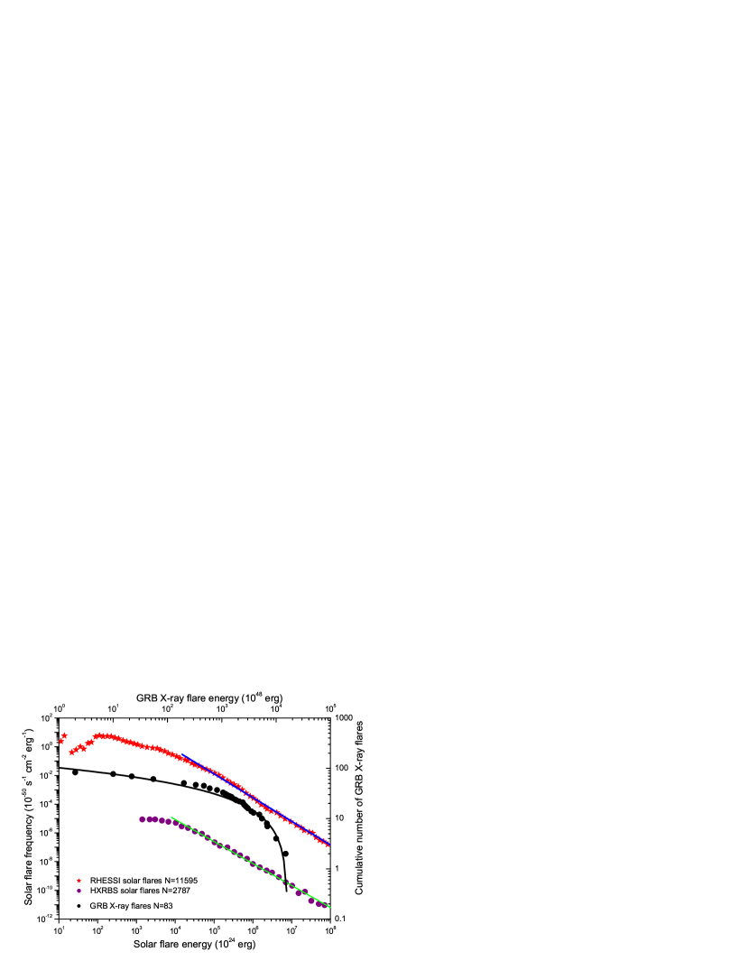
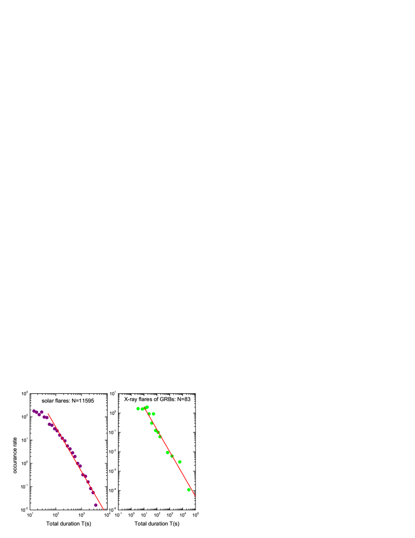
Figure 1 shows the cumulative energy distribution of GRB X-ray flares and the energy frequency distribution of solar hard X-ray flares. If the number of events $N(E)dE$ with energy between $E$ and $E+dE$ obeys a power-law relation, $N(E)dE\propto E^{-\alpha_{E}}dE$ for $E<E_{\rm max}$ , with index of $\alpha_{E}$ and cutoff energy of $E_{\rm max}$ , then we calculate the number of events with energy larger than $E$ through $N(>E)=a+b[E^{1-\alpha_{E}}-E_{\rm max}^{1-\alpha_{E}}]$ , where $a$ and $b$ are two parameters. In order to obtain the best-fitting parameters, the Markov chain Monte Carlo technique is used in our calculations. We obtain $\alpha_{E}\simeq 1.06\pm 0.15$ for GRB X-ray flares. In addition, the blue and green curves in Figure 1 represent the energy frequency distribution with $\alpha_{E}=1.65\pm 0.02$ and $1.53\pm 0.02$ for RHESSI[19] and HXRBS[20] solar flares, respectively. In Figure 2, we present the duration-time ( $T$ ) frequency distributions of solar flares and GRB X-ray flares, which can also be fitted by a power-law relation with index of $\alpha_{T}$ , i.e. $N(T)dT\propto T^{-\alpha_{T}}dT$ . The red lines in Figure 2 show a power-law fit with $\alpha_{T}=-1.10\pm 0.15$ and $-2.00\pm 0.05$ for GRB X-ray flares and solar flares, respectively.

Although the energy and duration-time frequency distributions for two kinds of flares are apparently different, we next show that these distributions can be well understood within one physical framework. The energy and duration frequency distributions of solar fares have been thought to be attributed to a magnetic reconnection process based on the fractal-diffusive avalanche model[19, 21, 23]. We further discuss this model to explain the energy and duration-time frequency distributions of GRB X-ray flares. For a self-organized criticality (SOC) avalanche, due to diffuse random walking, a statistical relationship[21] between size scale $L$ and duration time $T$ of the avalanche is $L\propto T^{1/2}$ , and a probability distribution of size $L$ is argued as $N(L)dL\propto L^{-S}dL$ for the three Euclidean dimensions $S=1$ , 2 and 3. This probability argument is based on the assumption that the occurrence frequency or number of events is equally likely throughout the system. So the index of the duration frequency distribution of flares is given by[21]

\alpha_{T}=\frac{S+1}{2}.

(1)

This index becomes $\alpha_{T}=1$ for $S=1$ and $\alpha_{T}=2$ for $S=3$ , which can well explain the observed duration distributions of GRB X-ray flares and solar flares. On the other hand, the index of the energy frequency distribution can be written by[21]

\alpha_{E}=\frac{3(S+1)}{S+5}.

(2)

It is easy to see that the index $\alpha_{E}=1$ for $S=1$ and $\alpha_{E}=1.5$ for $S=3$ , which are remarkably consistent with the observed indices of GRB X-ray flares and solar flares. A power-law distribution of occurrence frequency is characteristic of the SOC system[19]. According to equations (1) and (2), the power-law indices of the energy and duration-time distributions of SOC depend on the fractal geometry of the energy dissipation domain[21]. Thus, it is clear to find that GRB X-ray flares and solar flares correspond to the one-dimension ( $S=1$ ) and three-dimension ( $S=3$ ) cases, respectively. Therefore, GRB X-ray flares and solar flares share energy and duration-time frequency distributions, suggesting that they have a similar physical origin.

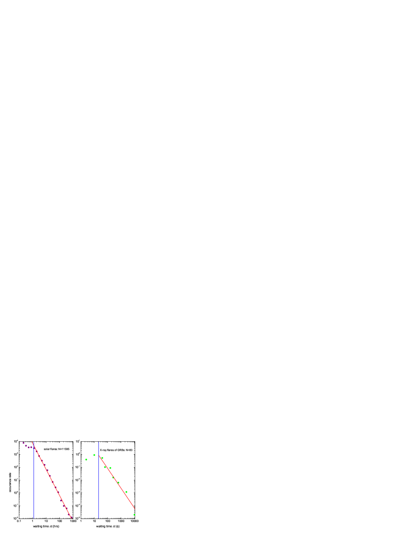
Now we discuss the waiting time distributions for two kinds of flares. The waiting time is defined as the time interval between two successive events. Its distribution tells us information on whether events occur as independent events, and provides the mean rate of event occurrence[19]. It has been suggested that the waiting time distribution of solar flares can be described by a power-law distribution with index of about $-2.0$ for long waiting times[22, 24]. But the waiting time distribution of GRB X-ray flares has not been studied before. Figure 3 displays the waiting time distribution of GRB X-ray flares and solar flares. Excluding the fluctuations of short waiting times, the waiting time distribution of GRB X-ray flares is also a power-law with index $-1.80\pm 0.20$ . The solar flares with waiting time larger than about 2 hours observed by RHEESI during 2002-2009 can be fitted by a power-law function with an index of $-2.0\pm 0.05$ . Thus, GRB X-ray flares and solar flares have similar waiting time distributions, which can be explained by non-stationary Poisson processes[22]. A Poissonian random process has an exponential waiting time distribution for a stationary flare rate and a power-law-like waiting time distribution for a non-stationary flare rate, which is the predication of the SOC theory[19]. For a non-stationary Poisson process, the waiting time distribution can be expressed by[22]

P(\Delta t)={\lambda_{0}\over(1+\lambda_{0}\Delta t)^{2}},

(3)

where $\lambda_{0}$ is the mean rate of flares. For large waiting times $(\Delta t\gg 1/\lambda_{0})$ , equation (3) approaches a power-law relation $P(\Delta t)\approx(1/\lambda_{0})(\Delta t)^{-2}$ , which is consistent with the observations. We can see from Figure 3 that the breakpoint is around $\Delta t_{0}=1/\lambda_{0}\sim 20$ s in the source’s rest frame for GRB X-ray flares (so the mean rate is $\lambda_{0}\sim 0.05\,{\rm s}^{-1}$ ), and $\Delta t_{0}\sim 1.2$ hrs for solar flares.

The statistical similarities between GRB X-ray flares and solar flares suggest a similar physical origin, i.e., magnetic reconnection. When and where does the magnetic reconnection event take place for an X-ray flare? The observations imply that the central engines of GRBs have long-lasting activity[2, 4, 5, 6, 7, 8] and X-ray flares arise from late internal shocks[25, 26], which could be formed through collisions of shells ejected after the prompt gamma-ray emission has ended. This implication is based on two following facts: first, the short rise and decay timescales and corresponding distributions of X-ray flares require that the central engines restart at late times[27], and second, the peak time of an X-ray flare observed by Swift is nearly equal to the ejection time of a relativistic outflow from the central engine if the decaying phase of the flare is understood as being due to the high latitude emission from the outflow[28]. Therefore, the magnetic reconnection event of an X-ray flare should occur at late times. Such an event could be powered by a differentially rotating, ultra-strongly magnetized, millisecond pulsar after the merger of a neutron star-neutron star binary or the collapse of a massive star[11]. The differential rotation leads to windup of poloidal magnetic fields in the interior and the resulting toroidal fields are strong enough to float up and break through the stellar surface[29, 30]. Magnetic reconnection-driven multiple explosions then occur, producing X-ray flares. Because these explosions usually take place around the pulsar’s surface along the rotation axis[29, 30], a cylinder-like magnetic-reconnection region with height $L$ has a volume $\sim\pi R_{\rm P}^{2}L$ (where $R_{\rm P}$ is the pulsar’s radius) and thus the probability distribution $N(L)$ is inversely proportional to $L$ . This implies that GRB X-ray flares belong to the one-dimension ( $S=1$ ) SOC case, as we found above. A variant of the magnetic reconnection mechanism is internal dissipation of relativistic winds from postburst millisecond magnetars (a type of pulsar with magnetic field strength of $\sim 10^{14}-10^{15}\,$ Gauss), which could account for the observational properties of GRB X-ray flares[12].

We have suggested the magnetic reconnection mechanism as the physical origin of GRB X-ray flares based on three statistical similarities between X-ray flares and solar flares. We found that such magnetic reconnection-driven events correspond to the $S=1$ SOC case for GRB X-ray flares. This is different from solar flares, which are thought to be due to a magnetic reconnection-driven $S=3$ SOC process[21]. Our work has at least three implications. First, it could not only help to understand the central engines of GRBs, but also help to study applications of solar magnetic-reconnection theories. Second, it could stimulate numerical simulations on a magnetic reconnection-driven self-organized criticality process under extreme astrophysical situations (e.g., ultra-strongly magnetized millisecond pulsars). Third, it could bring about similar statistical studies of other astrophysical explosive phenomena.

References

[1] Piro, L. et al. Probing the Environment in Gamma-Ray Bursts: The Case of an X-Ray Precursor, Afterglow Late Onset, and Wind Versus Constant Density Profile in GRB 011121 and GRB 011211, Astrophys. J. 623, 314-324 (2005).
[2] Burrows, D. N. et al. Bright X-ray Flares in Gamma-Ray Burst Afterglows, Science 309, 1833-1835 (2005).
[3] Barthelmy, S. D. et al. An origin for short $\gamma$ -ray bursts unassociated with current star formation, Nature 438, 994-996 (2005).
[4] Falcone, A. D. et al. The First Survey of X-Ray Flares from Gamma-Ray Bursts Observed by Swift: Spectral Properties and Energetics, Astrophys. J. 671, 1921-1938 (2007).
[5] Chincarini, C. et al. The First Survey of X-Ray Flares from Gamma-Ray Bursts Observed by Swift: Temporal Properties and Morphology, Astrophys. J. 671, 1903-1920 (2007).
[6] Chincarini, C. et al. Unveiling the origin of X-ray flares in gamma-ray bursts, Mon. Not. R. Astron. Soc. 406, 2113-2148 (2010).
[7] Margutti, R. et al. X-ray flare candidates in short gamma-ray bursts, Mon. Not. R. Astron. Soc. 417, 2144-2160 (2011).
[8] Bernardini, M. G., Margutti, R., Chincarini, C., Guidorzi, C. & Mao, J. Gamma-ray burst long lasting X-ray flaring activity, Astron. Astrophys. 526, A27-A35 (2011).
[9] Mészáros, P. Gamma-Ray Bursts, Rep. Prog. Phys. 69, 2259-2322 (2006).
[10] Zhang, B. Gamma-Ray Bursts in the Swift Era, Chin. J. Astron. Astrophys. 7, 1-50 (2007).
[11] Dai, Z. G., Wang, X. Y., Wu, X. F. & Zhang, B. X-ray flares from postmerger millisecond pulsars, Science 311, 1127-1129 (2006).
[12] Metzger, B. D., Giannios, D., Thompson, T. A., Bucciantini, N. & Quataert, E. The protomagnetar model for gamma-ray bursts, Mon. Not. R. Astron. Soc. 413, 2031-2056 (2011).
[13] Piran, T. The physics of gamma-ray bursts, Rev. Mod. Phys. 76, 1143-1210 (2004)
[14] Gehrels, N., Ramirez-Ruiz, E. & Fox, D. B. Gamma-Ray Bursts in the Swift Era, Ann. Rev. Astron. Astrophys. 47, 567-617 (2009).
[15] Kouveliotou, C. et al. Identification of two classes of gamma-ray bursts, Astrophys. J. 413, L101-L104 (1993).
[16] Gehrels, N. et al. The Swift Gamma-Ray Burst Mission, Astrophys. J. 611, 1005-1020 (2004).
[17] Shibata, K. & Magara, T. Solar Flares: Magnetohydrodynamic Processes, Living Rev. Solar Phys. 8, 6-104 (2011).
[18] Schaefer, B. E. The Hubble Diagram to Redshift $>6$ from 69 Gamma-Ray Bursts, Astrophys. J. 660, 16-46 (2007).
[19] Aschwanden, M. J. Self-Organized Criticality in Astrophysics: The Statistics of Nonlinear Processes in the Universe, Springer-Verlag: Berlin (2011).
[20] Crosby, N. B., Aschwanden, M. J. & Dennis, B. R. Frequency distributions and correlations of solar X-ray flare parameters, Solar Phys. 143, 275-299 (1993).
[21] Aschwanden, M. J. A statistical fractal-diffusive avalanche model of a slowly-driven self-organized criticality system, Astron. Astrophys. 539, A2 (2012).
[22] Aschwanden, M. J. & McTiernan, J. M. Reconciliation of Waiting Time Statistics of Solar Flares Observed in Hard X-Rays, Astrophys. J. 717, 683-692 (2010).
[23] Lu, E. T. & Hamilton, R. J. Avalanches and the distribution of solar flares, Astrophys. J. 380, L89-L92 (1991).
[24] Wheatland, M. S., Sturrock, P. A. & McTiernan, J. M. The Waiting-Time Distribution of Solar Flare Hard X-Ray Bursts, Astrophys. J. 509, 448-455 (1998).
[25] Fan, Y. Z. & Wei, D. M. Late internal-shock model for bright X-ray flares in gamma-ray burst afterglows and GRB 011121, Mon. Not. R. Astron. Soc. 364, L42-L46 (2005).
[26] Zhang, B. et al. Physical Processes Shaping Gamma-Ray Burst X-Ray Afterglow Light Curves: Theoretical Implications from the Swift X-Ray Telescope Observations, Astrophys. J. 642, 354-370 (2006).
[27] Lazzati, D. & Perna, R. X-ray flares and the duration of engine activity in gamma-ray bursts, Mon. Not. R. Astron. Soc. 375, L46-L50 (2007).
[28] Liang, E. W. et al. Testing the Curvature Effect and Internal Origin of Gamma-Ray Burst Prompt Emissions and X-Ray Flares with Swift Data, Astrophys. J. 646, 351-357 (2006).
[29] Kluźniak, W. & Ruderman, M. The Central Engine of Gamma-Ray Bursters, Astrophys. J. 505, L113-L117 (1998).
[30] Dai, Z. G. & Lu, T. $\gamma$ -Ray Bursts and Afterglows from Rotating Strange Stars and Neutron Stars, Phys. Rev. Lett. 81, 4301-4304 (1998).

Acknowledgements We thank M. J. Aschwanden, P. F. Chen, Y. Dai, M. D. Ding, Y. Guo, Y. F. Huang, and X. Y. Wang for discussions. This work was supported by the National Natural Science Foundation of China (grant No. 11103007 and 11033002).

Author Contributions F.Y.W. analyzed the observational data and explained the statistical results based on a self-organized criticality theory. Z.G.D. suggested such an analysis and proposed the physical origin of X-ray flares. Both authors wrote this paper together.

Author Information The authors declare that they have no competing financial interests. Correspondence and requests for materials should be addressed to Z.G.D. (dzg@nju.edu.cn) or F.Y.W. (fayinwang@nju.edu.cn).

Refer to caption — Figure 1: The cumulative energy distribution of GRB X-ray flares and the energy frequency distribution of solar hard X-ray flares. We employ 11595 solar flares[19] shown as red stars from RHESSI during 2002-2007, and 2787 flares[20] shown as purple dots from HXRBS during 1980-1982. The black curve gives the cumulative energy distribution $N(>E)=a+b[E^{1-\alpha_{E}}-E_{\rm max}^{1-\alpha_{E}}]$ . Using the Markov chain Monte Carlo fitting technique, we obtain $\alpha_{E}\sim 1.06\pm 0.15$ for GRB X-ray flares. For a differential frequency distribution $N(E)dE\propto E^{-\alpha_{E}}dE$ of solar flares, the blue and green curves give $\alpha_{E}=1.65\pm 0.02$ and $1.53\pm 0.02$ for the RHESSI and HXRBS samples, respectively. The magnetic reconnection process predicts that the value of $\alpha_{E}$ is $1.0$ and $1.5$ for one fractal dimension and three fractal dimensions, respectively[21]. Although the power-law indices are apparently different for GRB X-ray flares and solar flares, their physical mechanisms are similar, as discussed in the text.

Supplementary Information
Table S1. The measured parameters of X-ray flares of gamma-ray bursts.
Name	$z$	$t_{\rm start}^{\rm a}$	$T$ ^b	$S_{F}$	$E_{\rm iso}^{\rm c}$	Ref.
GRB		(s)	(s)	( $10^{-8}$ erg cm^-2)	( $10^{50}$ ergs)
050730	3.967	190.5	42.9	2.9	8.82	[6]
050730	3.967	311.6	110.7	10	30.4	[6]
050730	3.967	606.9	98.4	3.7	11.25	[6]
050908	3.344	362.4	115.9	1.9	4.4	[6]
060115	3.53	369.7	83.4	0.6	1.52	[6]
060210	3.91	136.5	60.7	23	68.40	[6]
060210	3.91	350.9	60.2	12	35.67	[6]
060418	1.489	122.3	25.1	48	27.01	[6]
060512	0.4428	167.4	79.3	4.5	0.22	[6]
060526	3.221	96.2	24.5	32	69.65	[6]
060526	3.221	257.5	37.7	25	54.41	[6]
060526	3.221	279.5	49.8	27	58.77	[6]
060526	3.221	316.8	71.9	13	28.30	[6]
060604	2.68	116.1	32.0	13	20.84	[6]
060604	2.68	163.7	21.9	7.9	12.67	[6]
060607A	3.082	92.1	15.9	4.4	8.91	[6]
060607A	3.082	193.0	75.5	24	48.59	[6]
060707	3.425	174.5	34.6	0.7	1.68	[6]
060714	2.711	55.6	8.2	3.8	6.21	[6]
060714	2.711	103.9	49.6	33	53.94	[6]
060714	2.711	131.5	14.0	9.5	15.53	[6]
060714	2.711	151.5	21.1	11	17.98	[6]
060729	0.54	163.4	43.7	93	6.99	[6]
060814	0.84	119.5	39.0	31	5.73	[6]
060904B	0.703	125.9	78.5	200	25.81	[6]
060908	1.8836	494.8	151.2	0.4	0.35	[6]
060908	1.8836	605.6	178.9	0.5	0.43	[6]
070306	1.4959	169.7	43.4	21	11.92	[6]
070318	0.836	179.0	28.9	1.0	0.18	[6]
070318	0.836	203.7	147.9	13.0	2.38	[6]
070721B	3.626	256.2	121.7	6.0	15.82	[6]
070721B	3.626	297.8	11.7	2.6	6.85	[6]
070721B	3.626	328.7	17.2	1.9	5.01	[6]
070721B	3.626	575.0	242.0	2.2	5.80	[6]
070724A	0.457	30.3	32.3	2.8	0.15	[6]
070724A	0.457	136.9	85.7	2.0	0.11	[6]
071031	2.692	66.6	61.2	9.5	15.35	[6]
071031	2.692	181.1	44.0	8.0	12.92	[6]
071031	2.692	242.8	51.9	5.4	8.72	[6]
071031	2.692	352.7	276.1	19.0	30.69	[6]
080210	2.641	153.9	35.7	9.3	14.54	[6]
080310	2.42	463.5	161.7	29.0	39.06	[6]
080310	2.42	526.5	59.6	18.0	24.25	[6]
050416A	0.654	1.5E6	5.0E5	3.4	0.38	[8]
060223A	4.41	891	293.0	0.9	3.23	[8]
060223A	4.41	1360	142.2	0.5	1.79	[8]
060906	3.69	908	5804	1.2	3.25	[8]
060906	3.69	6200	1459.0	0.5	1.36	[8]
070318	0.836	1.2E5	1.12E5	2.9	0.53	[8]
071031	2.692	4120	1745	0.2	0.32	[8]
071112C	0.82	296	187.5	1.8	0.32	[8]
071112C	0.82	810	224.9	1.2	0.21	[8]
090417B	0.35	1250	275.1	47.6	1.46	[8]
090417B	0.35	1420	217.8	45.1	1.38	[8]
090417B	0.35	1620	390.3	47.3	1.45	[8]
090809	2.74	2480	2667	6.9	11.48	[8]
050724	0.258	230	65.11	4.41	0.072	[7]
050724	0.258	9630	6.46E4	8.5	0.14	[8]
070724A	0.457	75	22.28	0.95	0.0507	[7]
070724A	0.457	90	19.1	1.26	0.067	[7]
070724A	0.457	150	87.8	1.83	0.097	[7]
071227	0.383	150	27.55	0.55	0.0203	[7]
100117A	0.92	130	42.77	0.98	0.2143	[7]
100117A	0.92	164	67.78	2.14	0.4745	[7]
100117A	0.92	200	22.11	0.40	0.0878	[7]
050802	1.434	312	145	0.2	0.10	[4]
050814	5.3	1133	841	0.2	0.95	[4]
050814	5.3	1633	944	0.4	1.90	[4]
050819	2.5	56	197	1.9	2.71	[4]
050819	2.5	9094	27628	1.0	1.42	[4]
050820A	2.617	200	182	68.1	104.8	[4]
050904	6.29	343	227	23.8	145.5	[4]
050904	6.29	857	284	1.6	9.78	[4]
050904	6.29	1149	194	1.0	6.11	[4]
050904	6.29	5085	3916	8.5	51.96	[4]
050904	6.29	16153	8713	10.7	65.41	[4]
050904	6.29	18383	20230	5.7	34.85	[4]
050904	6.29	25618	5360	4.1	25.06	[4]
050915A	2.53	55	115	2.7	3.93	[4]
060108	2.03	193	236	0.2	0.20	[4]
060108	2.03	4951	33035	7.0	6.93	[4]
060124	2.3	283	361	271.3	334.6	[4]
060124	2.3	644	363	124.0	153.0	[4]

Note: (a) In this table, the waiting time in the source frame can be obtained by $\Delta t=(t_{i+1}-t_{i})/(1+z)$ , where $t_{i+1}$ is the observed starting time of the $i+1$ th flare, and $t_{i}$ is the observed starting time of the $i$ th flare. For the first flare in one GRB, the waiting time is $t_{1}/(1+z)$ . (b) The flare duration time in the observer frame is $T$ , and the duration time in the source frame is $T/(1+z)$ . These flares are clearly distinguishable from the underlying continuum emission[4, 5, 6, 7, 8], so the duration suffers no bias. (c) The flare isotropic energy is calculated by $E_{\rm iso}=4\pi d^{2}_{L}(z)S_{F}/(1+z)$ , where $S_{F}$ is the fluence, and $d_{L}(z)$ is the luminosity distance calculated for a flat $\Lambda$ CDM universe with $\Omega_{M}=0.3$ , $\Omega_{\Lambda}=0.7$ and $H_{0}=70$ km s^-1 Mpc^-3.