Cavity-based robustness analysis of interdependent networks:
Influences of intranetwork and internetwork degree–degree correlations

Abstract

We develop a methodology for analyzing the percolation phenomena of two mutually coupled (interdependent) networks based on the cavity method of statistical mechanics. In particular, we take into account the influence of degree–degree correlations inside and between the networks on the network robustness against targeted (random degree-dependent) attacks and random failures. We show that the developed methodology is reduced to the well-known generating function formalism in the absence of degree–degree correlations. The validity of the developed methodology is confirmed by a comparison with the results of numerical experiments. Our analytical results indicate that the robustness of the interdependent networks depends on both the intranetwork and internetwork degree–degree correlations in a nontrivial way for both cases of random failures and targeted attacks.

I Introduction

There are many kinds of complex systems in both natural and artificial worlds, and recently these systems have come to be studied in various fields by being handled as networks. Networks are expressed mathematically as graphs in which the constituent elements and interactions among these elements are expressed as sites (nodes, vertices) and bonds (links, edges), respectively. Random networks in particular Erdos ; Bollobas , which are randomly generated networks characterized only by their macroscopic properties, have been widely examined because of their analytical tractability.

One major concern surrounding networks is the robustness against random failures (RFs) or targeted attacks (TAs). The size of the largest subset of sites that are connected to one another, which is often referred to as the giant component (GC) Jason , generally becomes smaller as more sites and/or bonds are removed. A standard measure to characterize the network robustness is the critical rate of failure at which the fraction of the GC against the size $N$ of the original network vanishes from $O(1)$ to zero; this is often referred to as the percolation threshold Kirkpatrick ; Callaway . In general, a network becomes more tolerant to RFs/TAs as each site in the network increases in degree, a parameter that represents the number of bonds directly connected to the site. On the other hand, increasing the number of bonds is generally costly in terms of various aspects. Therefore, several earlier studies examined the robustness of random networks that are specified by only the degree distribution while keeping the average degree fixed Valente ; Paul . However, the properties of real-world networks cannot be fully characterized by the degree distribution. As a logical step to take other statistical properties into account, the influences of degree correlations between two directly connected sites (degree–degree correlations) were also recently examined Shiraki ; Agliari ; Tanizawa .

More recently, a new type of model that considers interdependent networks was proposed Buldyrev 2010 ; Parshani PRL and has attracted significant attention Gao ; Son 2011 ; Morris ; Baxter ; Buldyrev 2011 ; Liu ; Zhou 2012 ; Schneider ; Parshani EPL ; Wang ; Min ; Cellai . In this model, the system is composed of two sub-networks in which the sites in one network are coupled with those in the other on a one-to-one basis. The two sites of a pair are dependent on each other, so that neither of the sites is functional (active) when either is broken (inactive). This interdependence between the two networks can facilitate a chain of failures, which is sometimes referred to as cascade phenomena; removal of sites in one network leads to the emergence of new isolated sites in the other, which then acts as a trigger of new failures in the first network and the process repeats itself. This mechanism can result in guidelines for constructing a robust system that are different from those known for single networks. For example, it is known that a broad degree distribution makes a network more robust against random site failures in the case of single networks Buldyrev 2011 , but in interdependent networks, the degrees in a network should be uniform to increase the network robustness when the interdependent site pairs are randomly coupled between the two networks because sites of a lower degree tend to cause catastrophic breakdowns that amplify the cascade phenomena Buldyrev 2010 . In a similar manner to the single-network case, the influences of degree–degree correlations in each network (intranetwork degree–degree correlations) have also been examined numerically Zhou 2012 . However, as far as the authors know, analytical examinations of the intracorrelations and correlations between networks (internetwork degree–degree correlations) have not yet been reported.

It is against this background that we develop here an analytical methodology for investigating the influences of the intra- and internetwork degree–degree correlations on the robustness of interdependent networks. Our method is based on the statistical mechanics cavity method developed for disordered systems Mezard 1987 ; Mezard 2001 ; Mezard 2009 and evaluates the probability that a pair of interdependent sites characterized by their degrees belongs to the GC by utilizing the tree approximation under the assumption that a GC of size $O(N)$ is formed.

The resultant methodology can be regarded as a generalization of the well-known generating function formalism (GFF) Newman 2001 that systematically evaluates various topological quantities by converting a graph into a transcendental equation of a single variable. One can analytically show that our methodology is reduced to the GFF in the absence of any degree correlations; solving a set of nonlinear equations with respect to multiple variables, which cannot be achieved with the standard GFF, is indispensable for evaluating the size of the GC in the presence of degree–degree correlations.

The remainder of this paper is organized as follows. In Sec. II, we briefly summarize the elemental concepts necessary for our investigation. In Sec. III, we develop our analytical methodology on the basis of the cavity method and discuss its relationship with the GFF. In Sec. IV, which is the main part of this paper, we demonstrate how the developed method is applied to interdependent networks, with the results for simple examples shown in Sec. V. We end the paper with a summary.

II Preliminaries on networks

We introduce here the definitions of several concepts that are necessary for our analysis of interdependent networks. We denote the degree distribution by $p(k)$, which indicates the fraction of sites of degree $k$ in a network. Based on this, we can define the degree distribution of a bond $r(k)$, which represents the probability that one terminal of a randomly chosen bond has degree $k$:

$$r(k)=\frac{kp(k)}{\sum_{l}lp(l)}=\frac{kp(k)}{\langle k\rangle},$$ (1)

where $\langle k\rangle$ is the average degree when a site in the network is chosen randomly.

Although the degree distribution is a fundamental feature, it is not sufficient to fully characterize the network properties Newman 2002 . For instance, social networks exhibit the assortative tendency that high-degree sites attach to other high-degree sites. In contrast, technological and biological networks exhibit the disassortative tendency that high-degree sites preferentially connect with low-degree sites, and vice versa. To introduce such tendencies in a simple manner, we characterize our network ensembles by utilizing the joint degree–degree distribution $r(k,l)$, which is the probability that the two terminal sites of a randomly chosen bond have degrees $k$ and $l$. From this definition, one can relate $r(k,l)$ to $p(k)$ and $r(k)$ as

$$\sum_{l}r(k,l)=r(k)=\frac{kp(k)}{\sum_{l}lp(l)},$$ (2)

for $\forall k$.

Furthermore, the joint distribution is used to evaluate the conditional distribution $r(k|l)$, i.e., the probability that one terminal site of a randomly chosen bond has degree $k$ given that the other terminal site has degree $l$, as

$$r(k|l)=\frac{r(k,l)}{r(l)}=\frac{\langle k\rangle r(k,l)}{lp(l)}.$$ (3)

When the condition

$$r(k|l)=r(k)$$ (4)

holds for $\forall k,l$, the degrees of the directly connected sites are statistically independent. To macroscopically quantify the degree–degree correlations, the Pearson coefficient

$$C=\frac{1}{\sigma^{2}_{r}}\sum_{kl}kl(r(k,l)-r(k)r(l)),$$ (5)

where

$$\sigma_{r}=\sum_{k}k^{2}r(k)-\left(\sum_{k}kr(k)\right)^{2}$$ (6)

is often used. If $C$ is zero, then the random network is regarded as uncorrelated. A positive (negative) $C$ indicates assortative (disassortative) mixing.

In a pair of interdependent networks, labeled A and B, we assume that each site in A is coupled with a site in B on a one-to-one basis. We represent the probability that a randomly chosen interdependent pair is composed of a site of degree $k_{\rm A}$ in A and a site of degree $k_{\rm B}$ in B as $P(k_{\rm A},k_{\rm B})$. Let us denote the joint degree–degree distribution for networks A and B as $r_{\rm A}({k_{\rm A}},l_{\rm A})$ and $r_{\rm B}({k_{\rm B}},l_{\rm B})$, respectively, For consistency, the identities

$$p_{\rm A}({k_{\rm A}}) = \sum_{{k_{\rm B}}}P(k_{\rm A},k_{\rm B})$$ (7)

$$r_{\rm A}({k_{\rm A}}) = \sum_{l_{\rm A}}r_{\rm A}({k_{\rm A}},l_{\rm A})=\frac{\sum_{{k_{\rm B}}}{k_{\rm A}}P({k_{\rm A}},{k_{\rm B}})}{\sum_{{k_{\rm A}},{k_{\rm B}}}{k_{\rm A}}P({k_{\rm A}},{k_{\rm B}})}$$ (8)

for network A, and those for network B, must hold. Using Bayes’ formula, the conditional distribution that a site in A has degree ${k_{\rm A}}$ under the condition that the coupled site in B has degree ${k_{\rm B}}$ is evaluated as

$$P_{\rm A}({k_{\rm A}}|{k_{\rm B}})=\frac{P({k_{\rm A}},{k_{\rm B}})}{\sum_{{k_{\rm B}}}P({k_{\rm A}},{k_{\rm B}})},$$ (9)

and

$$P_{\rm B}({k_{\rm B}}|{k_{\rm A}})=\frac{P({k_{\rm A}},{k_{\rm B}})}{\sum_{{k_{\rm A}}}P({k_{\rm A}},{k_{\rm B}})}.$$ (10)

Equations (8) and (10) are used for assessing the conditional distributions for site pairs; namely, the probability that a site pair of degrees $l_{\rm A}$ in A and $l_{\rm B}$ in B is connected with another site pair of degrees $k_{\rm A}$ in A and $k_{\rm B}$ in B by a link in A, which is evaluated as

$$r_{\rm A}(k_{\rm A},k_{\rm B}|l_{\rm A},l_{\rm B})=P_{\rm B}(k_{\rm B}|k_{\rm A})r_{\rm A}(k_{\rm A}|l_{\rm A}),$$ (11)

and $r_{\rm B}(k_{\rm A},k_{\rm B}|l_{\rm A},l_{\rm B})=P_{\rm A}(k_{\rm A}|k_{\rm B})r_{\rm B}(k_{\rm B}|l_{\rm B})$. These conditional distributions play an important role in analyzing interdependent networks.

In addition to this statistical characterization, we also handle a single realization of randomly generated networks. To specify such a network, we introduce the notation $\partial i$ for the set of all adjacent sites that are connected directly to site $i$ and $|\partial i|$ for the number of elements in $\partial i$. We use $X\backslash x$ to represent a set defined by removing an element $x$ from the set $X$. Therefore, $\partial i\backslash j$ refers to a set of sites that is defined by removing site $j\in\partial i$ from $\partial i$. For a pair of interdependent networks A and B, $\partial_{\rm A}i$ is used to represent the set of site pairs that are linked directly to the site pair $i$ in network A, with $\partial_{\rm B}i$ being that for network B.

We can also represent a network as a bipartite graph. For this, we denote site $i$ as a circle, an undirected link $a$ between two sites $i$ and $j$ as a square, and make a link for a related circle and square pair. This generally yields a bipartite graph in which each square has two links, while the number of links connected to a circle varies following a certain degree distribution (Fig. 1). In the bipartite graph expression, we denote $\partial a$ as the set of two circles connected to square $a$ and $\partial i$ as the set of squares connected to circle $i$. For a pair of interdependent networks A and B, $\partial_{\rm A}a$ and $\partial_{\rm A}i$ are used to represent the bipartite graph expression of the connectivity of site pairs in network A, and $\partial_{\rm B}a$ and $\partial_{\rm B}i$ are used for network B.

III Cavity approach to single networks

We review here the cavity approach to the robustness analysis of single complex networks, which was developed in an earlier study Shiraki . The relationship with the GFF Newman 2001 , another representative technique in research on complex networks, is also discussed.

III.1 Message passing algorithm: microscopic description

Let us suppose that a network that is sampled from an ensemble characterized by $p(k)$ and $r(k,l)$ suffers from RFs or TAs. We employ the binary variable $s_{i}\in\{0,1\}$ to represent whether site $i$ is active ($s_{i}=1$) or inactive ($s_{i}=0$) due to the failure. To take the connectivity into account, we introduce the state variable $\sigma_{i}\in\{0,1\}$, which indicates whether $\exists{j}\in\partial i$ belongs to the GC $(\sigma_{i}=0)$ or does not $(\sigma_{i}=1)$ when $i$ is left out. Using these definitions, $i$ is regarded as belonging to the GC if and only if $s_{i}(1-\sigma_{i})$ becomes unity, which gives the size of the GC as

$$S=\frac{1}{N}\sum_{i=1}^{N}s_{i}(1-\sigma_{i}).$$ (12)

Our analysis is based on the random-network property that the lengths of the closed paths between two randomly chosen sites (cycles) typically increase as $O(\ln N)$ as the size of the network $N$ tends to infinity, as long as the variance of the degree distribution is finite. This presumably holds even when the degree–degree correlations are introduced and indicates that we can locally handle a sufficiently large random network as a tree.

To incorporate this property in our analysis, we introduce the concept of an $i$-cavity system, which is defined by removing site $i$ from the original system. Let us define $m_{j\to i}=0$ when $\exists{h}\in\partial j$ belongs to the GC in the $i$-cavity system, and $m_{j\to i}=1$, otherwise. Then, $\sigma_{i}$ vanishes if and only if there exists a ${j}\in\partial i$ that is active $(s_{j}=1)$ and has $m_{j\to i}=0$. This offers the basic equation

$$\sigma_{i}=\prod_{j\in\partial i}\left(1-s_{j}+s_{j}m_{j\to i}\right).$$ (13)

Given an $i$-cavity system, we remove a site $j\in\partial i$ and switch $i$ back on instead, which yields a $j$-cavity system. Then, $m_{i\to j}$ vanishes if and only if $\exists{h}\in\partial i\backslash j$ belongs to the GC in the $j$-cavity system. A general and distinctive feature of trees is that when $i$ is removed, $\forall{j}\in\partial i$ are completely disconnected with one another. This indicates that $m_{i\to j}$ becomes unity if and only if none of ${h}\in\partial i\backslash j$ belongs to the GC in the $i$-cavity system. These definitions then provide the cavity equation:

$$m_{i\to j}=\prod_{h\in\partial i\backslash j}\left(1-s_{h}+s_{h}m_{h\to i}\right).$$ (14)

This equation defined for all links over the network determines the cavity variables $m_{j\to i}$ necessary for evaluating Eq. (13) for every site $i$. Solving Eq. (14) by the method of iterative substitution given the initial condition of $m_{j\to i}=0$ and substituting the obtained solution into Eq. (13) give the size of the GC, Eq. (12).

III.2 Bipartite graph expression

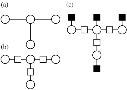
Figure 1: (a) Graph expression of a network. (b) Bipartite graph expression of the graph in (a). A square node is assigned for each edge in (a). (c) Bipartite graph expression of a damaged network. Black square nodes attached to each circle represent whether site $i$, denoted by the circle, is active $(s_{i}=1)$ or inactive $(s_{i}=0)$.

In general, the cavity equations are expressed as message passing algorithms on the bipartite graph corresponding to a given network Mezard 1987 . For this, we denote $1-s_{j}+s_{j}m_{j\to i}$ in two ways: $M_{j\to a}$ and $M_{a\to i}$, where $a$ represents a square connected to two circles $i$ and $j$. Using these, Eqs. (14) and (13) can also be expressed as

$$M_{a\to i} = M_{j\to a}\quad(\partial a=\{i,j\})$$ (15)

$$M_{i\to a} = 1-s_{i}+s_{i}\prod_{b\in\partial i\backslash a}M_{b\to i},$$ (16)

and

$$\sigma_{i}=\prod_{a\in\partial i}M_{a\to i},$$ (17)

respectively.

One advantage of this expression is that the influence of $s_{i}$ can be expressed graphically as an additional square node attached to circle $i$ (Fig. 1 (c)), which enables us to interpret Eqs. (15) and (16) as an algorithm that computes an outgoing message along a link from a node on the basis of incoming messages along the other links to the node. This type of interpretation is useful for constructing cavity equations to handle more advanced settings such as interdependent networks.

III.3 Macroscopic description

We turn now to an evaluation of the typical size of the GC when the networks are generated from an ensemble and damaged by RFs or TAs. We assume that, as a consequence of the failures, each site of degree $l$ is active only with a degree dependent probability $q_{l}$. We employ the bipartite graph expression, classify every site by its degree $l$, and define $I_{l}$ to be the frequency that sites of degree $l$ receive $M_{a\to i}=1$ among all links of the bipartite graph. Namely, $I_{l}$ is evaluated as $I_{l}=\left(l\sum_{i}\delta_{|\partial i|,l}\right)^{-1}\sum_{i}(\delta_{|\partial i|,l}\sum_{a\in\partial i}M_{a\to i})$, where the denominator is the number of links that connect to sites of degree $l$, and the numerator is the number of links for which $M_{a\to i}=1$ is received by sites of degree $l$.

Although $I_{l}$ has sample-to-sample fluctuations that depend on the network realizations, the strength of the fluctuations tends to zero as $N$ becomes larger. For typical samples, this indicates that the samples are expected to converge to their average as $N\to\infty$, a property known as self-averaging Mezard 1987 . In the current problem, because of the tree-like property of the random networks, $I_{l}$ can be evaluated as the expectations with respect to the graph and failure generations. In the bipartite graph expression, given a circle of degree $l$, the conditional distribution that the circle is coupled to a circle of degree $k$ through a square is given by $r(k|l)$. In addition, the probability that the circle of degree $k$ is active is $q_{k}$. Averaging Eq. (16) with respect to $r(k|l)$ and $q_{k}$ for a fixed value of $l$ and utilizing Eq. (15) leads to

$$I_{l}=\sum_{k}r(k|l)(1-q_{k}+q_{k}I_{k}^{k-1}).$$ (18)

Here, we have employed the property that the average of $\prod_{b\in\partial i\backslash a}M_{b\to i}$ on the right-hand side of Eq. (16) can be taken independently of the indices $b\in\partial i\backslash a$ because of the tree-like nature of random graphs. The whole set in Eq. (18) determines $I_{l}$ for $\forall{l}$. After solving the equations, the typical size of the GC is evaluated as

$$\mu=\sum_{l}p(l)q_{l}(1-I_{l}^{l}),$$ (19)

which corresponds to Eq. (12).

Equation (18) always allows a trivial solution $I_{l}=1$ for $\forall{l}$ yielding $\mu=0$. The local stability of this trivial solution can be evaluated by linearizing the equations, which gives

$$\delta I_{l}=\sum_{k}(k-1)q_{k}r(k|l)\delta I_{k},$$ (20)

or the alternative expression

$$\delta{\bf I}={\bf A}\delta{\bf I},$$ (21)

where $\bf A$ is a matrix defined as

$$A_{lk}=(k-1)q_{k}r(k|l).$$ (22)

Equation (21) states that the trivial solution is stable provided $\mu=0$ if and only if all eigenvalues of $\bf A$ are placed inside the unit circle centered at the origin in the complex plane. As $A_{lk}\geq 0$ is guaranteed for $\forall{l}$ and $\forall{k}$, the Perron-Frobenius theorem indicates that the critical condition changing this situation is given as

$${\rm det}\left({\bf E}-{\bf A}\right)=0,$$ (23)

which determines the percolation threshold for a given set of control parameters, where $\bf E$ is the identity matrix.

When the active probabilities $q_{l}$ are sufficiently small for $\forall{l}$, the absolute values of the eigenvalues of $\bf A$ become so small that the trivial solution is guaranteed to be stable, yielding a vanishingly small GC size of $\mu=0$. However, as the values of $q_{l}$ become larger in a certain manner, Eq. (23) is satisfied at the percolation threshold, and a solution of $\mu>0$ comes continuously from the trivial solution. In this way, the emergence of a large GC is always described as a continuous phase transition for single networks.

III.4 Connection between the cavity method and generating function formalism

Before proceeding further, we mention briefly the relationship between the cavity method and the GFF.

Consider the cases of no degree correlations $r(k|l)=r(k)$ for arbitrary pairs of ${k,l}$ and no site dependence of the active probability $q_{l}=q$ for $\forall{l}$. In such cases, Eq. (18) becomes independent of $l$, and therefore we can set $I_{l}=I$. This makes it possible to summarize Eq. (18) as

$$\sum_{l}r(l)I^{l-1}=\sum_{l}r(l)\left(1-q+q\sum_{k}r(k)I^{k-1}\right)^{l-1},$$ (24)

which can be expressed more concisely as

$$f=H(1-q+qf),$$ (25)

where we have defined

$$G(x) = \sum_{k}p(k)x^{k},$$ (26)

$$H(x) = \sum_{k}r(k)x^{k-1}=\frac{G^{\prime}(x)}{G^{\prime}(1)},$$ (27)

and set $f\equiv\sum_{k}r(k)I^{k-1}=H(I)$. Using the solution of Eq. (25), Eq. (19) is evaluated as

$$\mu=q\left(1-G(1-q+qf)\right).$$ (28)

Equation (25) is nothing but a transcendental equation for the GFF Buldyrev 2011 . Namely, the cavity method is reduced to the GFF in the simplest cases. However, when degree–degree correlations exist, $I_{l}$ generally depends on the degree $l$, and therefore the cavity equations, Eq. (18), cannot be summarized as a nonlinear equation of a single variable. As a consequence, one cannot exploit the compact expression of the GFF and has to directly deal with the cavity equations for evaluating the size of the GC Shiraki ; Tanizawa . A similar idea has been implemented in the GFF by handling a set of coupled generating functions for evaluating the GC of networks free from failures Newman 2002 .

IV Cavity approach for interdependent networks

In this section, we develop the cavity method for analyzing the cascade phenomena in interdependent networks that occurs as a result of RFs or TAs.

IV.1 Cascade phenomena of interdependent networks

Consider the pair of interdependent networks introduced in Sec. II. Each pair of sites in networks A and B is interdependent so that both sites become inactive and lose their functions if one site becomes inactive. In addition, each active site in A also loses its function if it is disconnected from the GC of A, which brings about functional failure of the coupled site in B, and vice versa. In each network, the GC is defined as the largest subset of functional sites.

We assume initial conditions of all sites being active and functional in both networks. In the initial step, sites in A suffer from RFs or TAs, and only a portion of the sites remain active. Further, an additional portion of sites lose their functions because they were disconnected from the GC of A. In the second step, the sites in B that are coupled with the sites in A that were disconnected from the GC also lose their functions due to the properties of interdependent networks noted above. This reduces the size of the GC in B, and an extra potion of sites in B lose their functions. In the third step, functional failure in B is propagated back to A causing further functional failure in A, and this process is repeated until convergence. This is the cascade phenomena.

At convergence, every site of the GC in A is coupled with a site of the GC in B on a one-to-one basis. The resulting GC of the site pairs is often termed the mutual GC. Earlier studies reported that unlike the case of single networks, the size of the mutual GC relative to the network size vanishes discontinuously from $O(1)$ to zero at a critical condition as the strength of the failures in the initial step becomes larger Buldyrev 2010 ; Parshani PRL . We develop here a methodology for examining this phenomena on the basis of the cavity method by taking degree–degree correlations into account.

IV.2 Microscopic description

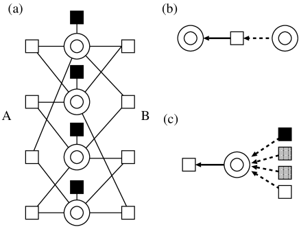
Figure 2: (a) Bipartite graph expression of interdependent networks. Double circles represent site pairs connected by internetwork links. White squares represent links in each network, while each black square represents whether the site in A of the site pairs is removed in the initial failure or not. (b) Graphical expression of Eq. (30) in A and Eq. (33) in B. (c) Graphical expression of Eq. (31) in A and Eq. (34) in B. Shaded squares indicate square nodes in the counterpart network, messages from which are evaluated in the previous step and fixed in the current update. Messages from the black squares are fixed as $s_{i}$ in all steps. Contributions from the shaded and black squares are summarized as $\tau_{{\rm A},i}^{2t-1}$ and $\tau_{{\rm B},i}^{2t}$ in Eq. (31) and Eq. (34), respectively. In (b) and (c), the message of the full line is computed from message(s) of the broken line(s).

Let us denote a site pair of the interdependent networks as $i$. We employ a binary variable $s_{i}\in\{0,1\}$ to represent whether $i$ is kept active in the initial stage $(s_{i}=1)$ or fails $(s_{i}=0)$. We also introduce the state variable $\sigma_{{\rm A},i}^{t}\in\{0,1\}$ that indicates whether $\exists{j}\in\partial_{\rm A}i$ belongs to the GC in A $(\sigma_{i}^{\rm A}=0)$ or does not $(\sigma_{i}^{\rm A}=1)$ when $i$ is left out after the $t$-th $(t=1,2,\ldots)$ step, with $\sigma_{{\rm B},i}$ being the equivalent state variable for B. Using these, the size of the mutual GC after the $2t$-th step is expressed as

$$S^{2t}=\frac{1}{N}\sum_{i=1}^{N}s_{i}(1-\sigma_{{\rm A},i}^{2t-1})(1-\sigma_{{\rm B},i}^{2t}).$$ (29)

For a given $t$, $\sigma_{{\rm A},i}^{2t-1}$ and $\sigma_{{\rm B},i}^{2t}$ can be obtained by the cavity method. To do this, we note that the state variables in A after the $2t-1$-th step can be evaluated by the scheme for single networks by handing $\tau_{{\rm A},i}^{2t-1}=s_{i}(1-\sigma_{{\rm B},i}^{2t-2})$ as a binary variable for representing whether $i$ is active $(\tau_{{\rm A},i}^{2t-1}=1)$ or inactive $(\tau_{{\rm A},i}^{2t-1}=0)$, where $\sigma_{{\rm B},i}^{0}$ is set to zero from the assumption. Using the bipartite graph expression (Fig. 2), we get

$$M_{a\to i}^{\rm A} = M_{j\to a}^{\rm A}\quad\left(\partial_{\rm A}a=\{i,j\}\right),$$ (30)

$$M_{i\to a}^{\rm A} = \!1\!-\!\tau_{{\rm A},i}^{2t-1}\!+\!\tau_{{\rm A},i}^{2t-1}\!\prod_{b\in\partial_{\rm A}i\backslash a}M_{b\to i}^{\rm A},$$ (31)

and the solution of these yields

$$\sigma_{{\rm A},i}^{2t-1}=\prod_{a\in\partial_{\rm A}i}M_{a\to i}^{\rm A}.$$ (32)

Similarly, those in B after the $2t$-th step are

$$M_{a\to i}^{\rm B} = M_{j\to a}^{\rm B}\quad\left(\partial_{\rm B}a=\{i,j\}\right),$$ (33)

$$M_{i\to a}^{\rm B} = \!1\!-\!\tau_{{\rm B},i}^{2t}\!+\!\tau_{{\rm B},i}^{2t}\!\prod_{b\in\partial_{\rm B}i\backslash a}M_{b\to i}^{\rm B},$$ (34)

and

$$\sigma_{{\rm B},i}^{2t}=\prod_{a\in\partial_{\rm B}i}M_{a\to i}^{\rm B},$$ (35)

where we set $\tau_{{\rm B},i}^{2t}=s_{i}(1-\sigma_{{\rm A},i}^{2t-1})$. Solving these with the initial conditions $M_{i\to a}^{\rm A}=0$ or $M_{i\to a}^{\rm B}=0$ at each step and inserting the resultant values of Eqs. (32) and (35) into Eq. (29) offer the size of the GC after the $2t$-th step for a given sample of interdependent networks and initial failures.

IV.3 Macroscopic description

To evaluate the typical size of the mutual GC when the interdependent networks are generated as mentioned in Sec. II and suffer from RFs or TAs, we assume that each site pair of degrees $l_{\rm A}$ in A and $l_{\rm B}$ in B is kept active with a degree pair dependent probability $q_{l_{\rm A}l_{\rm B}}$ as a consequence of the failures that are brought about in network A at the initial stage. For RFs, we set

$$\!q_{l_{\rm A}l_{\rm B}}\!=q,$$ (36)

which implies that failures are generated randomly irrespectively of the values of $l_{\rm A}$ and $l_{\rm B}$. On the other hand, TAs are made preferentially for sites of the larger degrees in network A. Therefore, for a given value of the average active rate $q$, we assign the values of $q_{l_{\rm A}l_{\rm B}}$ as

$$q_{l_{\rm A}l_{\rm B}}=\left\{\begin{array}[]{ll}0&(l_{\rm A}>\Theta)\cr\Delta&(l_{\rm A}=\Theta),\\ 1&(l_{\rm A}<\Theta)\end{array}\right.$$ (40)

where $\Theta$ and $\Delta$ are uniquely determined so that

$$q=\sum_{l_{\rm B}}\left(\Delta P(\Theta,l_{\rm B})+\sum_{l_{\rm A}<\Theta}P(l_{\rm A},l_{\rm B})\right)$$ (41)

holds.

The key idea of our analysis is basically the same as that for single networks; namely, we describe the system using conditional frequencies that a site pair characterized by a pair of degrees $l_{\rm A}$ in A and $l_{\rm B}$ in B receives messages of unity from connected links in A and B. For this, we define $I^{\rm A}_{l_{\rm A}l_{\rm B}}\!=\!\left(l_{\rm A}\!\sum_{i}\delta_{|\partial_{\rm A}i|,l_{\rm A}}\delta_{|\partial_{\rm B}i|,l_{\rm B}}\right)^{-1}\!\left(\!\sum_{i}\!\delta_{|\partial_{\rm A}i|,l_{\rm A}}\!\sum_{a\in\partial i}\!M_{a\to i}^{\rm A}\!\right)$, and similarly define $I^{\rm B}_{l_{\rm A}l_{\rm B}}$ for B.

Let us denote $q_{{\rm A},l_{\rm A}l_{\rm B}}^{2t-1}$ as the conditional probability that $\tau_{{\rm A},i}^{2t-1}$ takes a value of unity for site pairs of degrees $l_{\rm A}$ in A and $l_{\rm B}$ in B at the $2t-1$-th step. The self-averaging property and the tree-like nature of random graphs allow us to macroscopically describe Eqs. (30) and (31) as

$$I^{\rm A}_{l_{\rm A}l_{\rm B}}=\!\sum_{k_{\rm A},k_{\rm B}}\!r_{\rm A}\!(k_{\rm A},\!k_{\rm B}|l_{\rm A},\!l_{\rm B})$$ (42)

$$\hskip 42.67912pt\times\left(\!1\!-\!q_{{\rm A},k_{\rm A}k_{\rm B}}^{2t\!-\!1}\!+\!q_{{\rm A},k_{\rm A}k_{\rm B}}^{2t\!-\!1}(I^{\rm A}_{k_{\rm A}k_{\rm B}})^{k_{\rm A}-1}\!\right).$$ (43)

Equation (32) states that the conditional probability of a site pair of degrees $l_{\rm A}$ in A and $l_{\rm B}$ in B having $\sigma_{{\rm A},i}^{2t-1}=1$ after the $2t-1$-th step is $\left(I^{\rm A}_{l_{\rm A}l_{\rm B}}\right)^{l_{\rm A}}$. Among these sites, only the fraction of $q_{l_{\rm A}l_{\rm B}}$ is active. Therefore, the conditional probability that a site pair of degrees $l_{\rm A}$ in A and $l_{\rm B}$ in B has $\tau_{{\rm B},i}^{2t}=1$ in B at the $2t$-th step is evaluated as

$$q_{{\rm B},l_{\rm A}l_{\rm B}}^{2t}=q_{l_{\rm A}l_{\rm B}}\left(1-\left(I^{\rm A}_{l_{\rm A}l_{\rm B}}\right)^{l_{\rm A}}\right),$$ (44)

using the solution of Eq. (43). Equation (44) makes it possible to macroscopically describe the cavity equation in B at the $2t$-th step in a similar manner to Eq. (43) as

$$I^{\rm B}_{l_{\rm A}l_{\rm B}}=\!\sum_{k_{\rm A},k_{\rm B}}\!r_{\rm B}\!(k_{\rm A},\!k_{\rm B}|l_{\rm A},\!l_{\rm B})$$ (45)

$$\hskip 42.67912pt\times\left(\!1\!-\!q_{{\rm B},k_{\rm A}k_{\rm B}}^{2t}\!+\!q_{{\rm B},k_{\rm A}k_{\rm B}}^{2t}(I^{\rm B}_{k_{\rm A}k_{\rm B}})^{k_{\rm B}-1}\!\right).$$ (46)

Using the solution of Eq. (46), the conditional probability that a site pair of degrees $l_{\rm A}$ in A and $l_{\rm B}$ in B has $\tau_{{\rm A},i}^{2t+1}=1$ in A at the $2t+1$-step is evaluated as

$$q_{{\rm A},l_{\rm A}l_{\rm B}}^{2t+1}=q_{l_{\rm A}l_{\rm B}}\left(1-\left(I^{\rm B}_{l_{\rm A}l_{\rm B}}\right)^{l_{\rm B}}\right).$$ (47)

Equation (29) gives the expectation of the size of the mutual GC after the $2t$-th step as

$$\mu^{2t}=\sum_{l_{\rm A},l_{\rm B}}P(l_{\rm A},l_{\rm B})q_{l_{\rm A}l_{\rm B}}\left(1-\left(I^{\rm A}_{l_{\rm A}l_{\rm B}}\right)^{l_{\rm A}}\right)$$ (48)

$$\hskip 56.9055pt\times\left(1-\left(I^{\rm B}_{l_{\rm A}l_{\rm B}}\right)^{l_{\rm B}}\right)$$ (49)

$$\phantom{\mu^{2t}}=\sum_{l_{\rm A},l_{\rm B}}P(l_{\rm A},l_{\rm B})\left(q_{l_{\rm A}l_{\rm B}}\right)^{-1}q_{{\rm A},l_{\rm A}l_{\rm B}}^{2t-1}q_{{\rm B},l_{\rm A}l_{\rm B}}^{2t}.$$ (50)

Equations (43)–(50) constitute the main result of the present paper.

One thing is noteworthy here. Similar to the case of single networks, Eq. (43) always allows a trivial solution of $I_{l_{\rm A}l_{\rm B}}^{\rm A}=1$, which becomes stable when sufficiently small $q_{{\rm A},l_{\rm A}l_{\rm B}}^{2t-1}$ values are set for all pairs of $l_{\rm A}$ and $l_{\rm B}$. This yields $q_{{\rm B},l_{\rm A}l_{\rm B}}^{2t}=0$ for all pairs of $l_{\rm A}$ and $l_{\rm B}$ in Eq. (44), which makes $I_{l_{\rm A}l_{\rm B}}^{\rm B}=1$ the unique and stable solution of Eq. (46) at the $2t$-th step, offering $\mu^{2t}=0$. In addition, at the subsequent $2t+1$-th step, $q_{{\rm A},l_{\rm A}l_{\rm B}}^{2t+1}=0$ holds for all pairs of $l_{\rm A}$ and $l_{\rm B}$, which once more guarantees that the trivial solution is stable. This means that unlike the case of single networks, the trivial solution of $\mu^{*}=\lim_{t\to\infty}\mu^{2t}=0$ is always locally stable in the dynamics of Eqs. (43)–(47) irrespective of the strength of the RFs. A finite $\mu^{*}$ is obtained when sufficiently large $q_{{\rm A},l_{\rm A}l_{\rm B}}^{1}=q_{l_{\rm A}l_{\rm B}}$ values are set in the initial step for all pairs of $l_{\rm A}$ and $l_{\rm B}$. As a consequence, the transition of a finite value of $\mu^{*}$ to zero generally occurs in a discontinuous manner for interdependent networks even when degree–degree correlations are taken into account. Earlier studies, however, have already reported the occurrence of the discontinuous transition for a few specific examples Buldyrev 2010 ; Buldyrev 2011 ; Zhou 2012 .

IV.4 Relationship with earlier studies

In Ref. Buldyrev 2011 , the case involving the highest internetwork degree–degree correlation ($P(k_{\rm A},k_{\rm B})=\delta_{k_{\rm B},k_{\rm A}}p(k_{\rm A})$) and no intranetwork degree–degree correlation ($r_{\rm A}(k,l)=r_{\rm B}(k,l)=r(k)r(l)$) is examined for degree-independent RFs characterized by $q_{l_{\rm A}l_{\rm B}}=q$. In such a case, we can assume that $I_{l_{\rm A}l_{\rm B}}^{\rm A}=I_{l_{\rm A}l_{\rm B}}^{\rm B}=I$, ignoring the dependence on the degree and network. Further, we can set $\lim_{t\to\infty}q_{{\rm A},ll}^{2t-1}=\lim_{t\to\infty}q_{{\rm B},ll}^{2t}=q(1-I^{l})$ because of the symmetry between networks A and B. Inserting these into Eq. (43), in conjunction with $r_{\rm A}(k_{\rm A},k_{\rm B}|l_{\rm A},l_{\rm B})=\delta_{k_{\rm B},k_{\rm A}}r(k_{\rm A})\delta_{l_{\rm A},l_{\rm B}}$, we obtain an equation concerning $I$:

$$I = 1-q\left(1-IH(I)\right)+q\left(H(I)-IH(I^{2})\right)$$ (51)

$$= 1-q\left(1-(I+1)H(I)+IH(I^{2})\right),$$ (52)

which is equivalent to Eq. (36) in Ref. Buldyrev 2011 . The size of the mutual GC for $t\to\infty$ is evaluated by inserting $I_{l_{\rm A}l_{\rm B}}^{\rm A}=I_{l_{\rm A}l_{\rm B}}^{\rm B}=I$ into Eq. (50) for $P(k_{\rm A},k_{\rm B})=\delta_{k_{\rm B},k_{\rm A}}p(k_{\rm A})$. This provides the expression

$$\mu^{*}=q\left(1-2G(I)+G(I^{2})\right),$$ (53)

which is also equivalent to Eq. (35) in Ref. Buldyrev 2011 .

In Ref. Buldyrev 2010 , the case of no intranetwork degree–degree correlation ($r_{\rm A}(k,l)=r_{\rm A}(k)r_{\rm A}(l)$, $r_{\rm B}(k,l)=r_{\rm B}(k)r_{\rm B}(l)$) and no internetwork degree–degree correlation ($P(k_{\rm A},k_{\rm B})=p_{\rm A}(k_{\rm A})p_{\rm B}(k_{\rm B})$) is discussed. In such a case, one can set $I_{l_{\rm A}l_{\rm B}}^{\rm A}=I_{\rm A}$ and $I_{l_{\rm A}l_{\rm B}}^{\rm B}=I_{\rm B}$ by ignoring the site dependence. Let us focus on the case of degree independent RFs $q_{l_{\rm A}l_{\rm B}}=q$ and the convergent state. Inserting $r_{\rm A}(k_{\rm A},k_{\rm B}|l_{\rm A},l_{\rm B})=p_{\rm B}(k_{\rm B})r_{\rm A}(k_{\rm A})$ into Eq. (43) yields

$$I_{\rm A} = 1-q_{\rm B}+q_{\rm B}\left(\sum_{k_{\rm A}}r_{\rm A}(k_{\rm A})I_{\rm A}^{k_{\rm A}-1}\right)$$ (54)

$$= 1-q_{\rm B}+q_{\rm B}f_{\rm A},$$ (55)

or alternatively

$$f_{\rm A}=H_{\rm A}(1-q_{\rm B}+q_{\rm B}f_{\rm A}),$$ (56)

where $H_{\rm A}(x)=\sum_{k}r_{\rm A}(k)x^{k-1}$ and $f_{\rm A}=H_{\rm A}(I_{\rm A})$. In a similar manner, Eq. (46) offers

$$f_{\rm B}=H_{\rm B}(1-q_{\rm A}+q_{\rm A}f_{\rm B}),$$ (57)

where $H_{\rm B}(x)=\sum_{k}r_{\rm B}(k)x^{k-1}$. Equations (47) and (44) provide $q_{\rm A}$ and $q_{\rm B}$ in Eqs. (56) and (57) in a self-consistent manner as

$$q_{\rm A} = q\left(1-\sum_{k}p_{\rm A}(k)I_{\rm A}^{k}\right)$$ (58)

$$= q\left(1-G_{\rm A}(1-q_{\rm B}+q_{\rm B}f_{\rm A})\right)$$ (59)

and

$$q_{\rm B}=q\left(1-G_{\rm B}(1-q_{\rm A}+q_{\rm A}f_{\rm B})\right),$$ (60)

respectively, where $G_{\rm A}(x)=\sum_{k}p_{\rm A}(k)x^{k}$ and $G_{\rm B}(x)=\sum_{k}p_{\rm B}(k)x^{k}$. Equations (56)–(60) constitute a set of conditions for determining four variables: $f_{\rm A},f_{\rm B},q_{\rm A}$, and $q_{\rm B}$. Using these variables, the size of the mutual GC is evaluated as

$$\mu^{*}=q\left(1-G_{\rm A}(1-q_{\rm B}+q_{\rm B}f_{\rm A})\right)$$ (61)

$$\hskip 56.9055pt\times\left(1-G_{\rm B}(1-q_{\rm A}+q_{\rm A}f_{\rm B})\right).$$ (62)

For Erdös-Renyi ensembles in particular, which are characterized by $p_{\rm A}(k)=e^{-a}a^{k}/k!$ and $p_{\rm B}(k)=e^{-b}b^{k}/k!$, Eqs. (56)–(60) can be summarized as two equations, since $G_{\rm A}(x)$ and $G_{\rm B}(x)$ accord to $H_{\rm A}(x)$ and $H_{\rm B}(x)$, respectively, as $G_{\rm A}(x)=H_{\rm A}(x)=\exp(a(x-1))$ and $G_{\rm B}(x)=H_{\rm B}(x)=\exp(b(x-1))$. The resultant coupled equations can be read as

$$f_{\rm A}=\exp\left(-a(f_{\rm A}-1)(f_{\rm B}-1)\right)$$ (63)

and

$$f_{\rm B}=\exp\left(-b(f_{\rm A}-1)(f_{\rm B}-1)\right),$$ (64)

which are identical to Eq. (14) in the Supplemental Material of Ref. Buldyrev 2010 .

These two examples show that our scheme can be expressed compactly using the generating functions when the macroscopic cavity variables $I^{\rm A}_{l_{\rm A}l_{\rm B}}$ and $I^{\rm B}_{l_{\rm A}l_{\rm B}}$ are independent of the degrees $l_{\rm A}$ and $l_{\rm B}$ as a consequence of the assumed statistical features of objective systems and failures. However, correlations of the degrees and/or site dependence of the failures induces degree dependence of the macroscopic cavity variables. In such cases, one has no choice but to directly handle Eqs. (43)–(50) to theoretically describe the behavior of interdependent networks.

V Numerical tests and results

V.1 The flow

To confirm the validity of the analytical scheme, we carried out numerical experiments using interdependent networks of $N=10000$ characterized by a set of joint degree distributions $P(k_{\rm A},k_{\rm B})$, $r_{\rm A}(k_{\rm A},l_{\rm A})$, and $r_{\rm B}(k_{\rm B},l_{\rm B})$ on the basis of the Monte Carlo algorithm proposed in Ref. Newman 2002 . We measured the size of the GC, using the algorithm proposed in Ref. Hoshen ; Al-Futaisi . To trigger the cascade phenomena, sites in the constructed network A were removed randomly (RF) or preferentially (TA). In each case, we evaluated the size of the mutual GC after convergence and compared it with the analytical solution obtained by the cavity method.

As a simple but nontrivial example, we focused on two-peak models where the fractions of larger and smaller degrees are fifty-fifty. We set the values of the larger and smaller degrees as $6$ and $4$, respectively, for both of networks A and B. In such models, the intranetwork degree–degree correlations can be uniquely specified by the Pearson coefficient, which is denoted as $C_{\rm A}$ and $C_{\rm B}$ for sub-networks A and B, respectively. However, the influence of the internetwork degree–degree correlations between networks A and B cannot be fully characterized by only the Pearson coefficient of $P(k_{\rm A},k_{\rm B})$, denoted as $C_{\rm I}$, because pairs of $(k_{\rm A}=4,k_{\rm B}=6)$ and $(k_{\rm A}=6,k_{\rm B}=4)$ are affected by the initial removal in different ways for TAs. However, for brevity, we suppose that the fraction of these pairs are the same, which enables us to characterize the intra- and internetwork degree–degree correlations by three parameters” $(C_{\rm A},C_{\rm B},C_{\rm I})$.

The manner in which the failures occur also influences the size of the mutual GC. In the case of RF, the randomness of the initial removal means that the initial survival probability of the site pairs does not depend on their degree pairs. For a TA, however, site pairs that have a higher degree in A are removed preferentially, and how the removal influences the sites in B in the first stage depends on the internetwork degree–degree correlation. This implies that the robustness of the interdependent networks can depend on the internetwork degree–degree correlations in a nontrivial manner.

V.2 Results and discussion

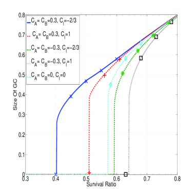
Figure 3: (Color online) Cascade phenomena of two-peak interdependent networks triggered by a TA. Each symbol represents the size of the mutual GC evaluated from 50 experiments for networks of $N=10000$. Statistical errors are smaller than the size of the symbols.

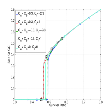
Figure 4: (Color online) Cascade phenomena of two-peak interdependent networks triggered by a RF. Each symbol represents the size of the mutual GC evaluated from 50 experiments for networks of $N=10000$. Statistical errors are smaller than the size of the symbols.

Figures 3 and 4 show how the size of the mutual GC depends on the fraction of initial failures in the cases of TAs and RFs, respectively. The solid lines represent estimates obtained from the cavity method, while the symbols denote the results of the numerical experiments. The results are in agreement with an excellent accuracy, which validates our cavity-based analytical scheme. The figures indicate that the percolation transition of the interdependent networks remains discontinuous irrespective of the introduction of the intra- and/or internetwork degree–degree correlations.

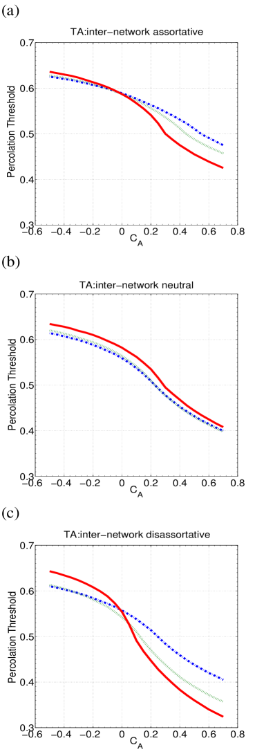
Figure 5: (Color online) Percolation threshold as a function of the Pearson coefficient of network A, $C_{\rm A}$, in the case of a TA; (a), (b), and (c) correspond to three different values of the Pearson coefficient for the internetwork degree–degree correlations $C_{\rm I}=0.5$, $0$, and $-0.5$, respectively. Results are shown for different values of the Pearson coefficient of network B $C_{\rm B}$: $0.7$ (solid red line; assortative), $0$ (dashed green line; neutral), and $-0.5$ (dash-dotted blue line: disassortative).

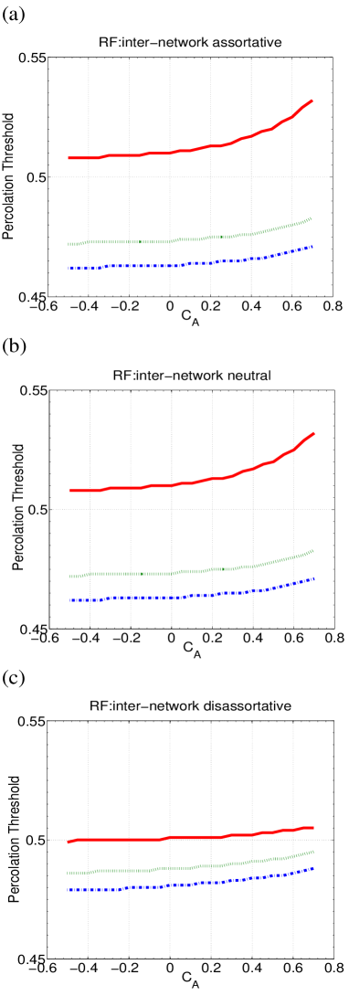
Figure 6: (Color online) Percolation threshold as a function of the Pearson coefficient of network A, $C_{\rm A}$, in the case of RF. The same lines as those described in the legend of Fig. 5 are used.

Figures 5 (a)–(c) show how the percolation threshold depends on the intranetwork degree correlations for a TA. The results indicate that the percolation threshold depends strongly on the various degree correlations, and the interdependent networks become more tolerant by introducing assortative intranetwork degree–degree correlations to each network in the presence of the internetwork degree–degree correlations, whether they are assortative [Fig. 5 (a)] or disassortative [Fig. 5 (c)]. In the absence of internetwork degree–degree correlations [Fig. 5 (b)], however, the networks are the most tolerant when the intranetwork degree–degree correlations in A are assortative and those in B are disassortative.

A significantly different dependence on the intranetwork degree–degree correlations is observed for RF. Figures 6 (a)–(c) indicate that whatever type of internetwork degree–degree correlation is introduced, disassortative intranetwork degree–degree correlations in both networks A and B provide the highest robustness. However, as a whole, the change in the percolation threshold as a function of the various degree–degree correlations is relatively small. This indicates that the role of the degree–degree correlations is not significant in the case of RF, which is in contrast to the case of TA.

Finally, we tested cases of various degree combinations using the cavity method. Tables 1 and 2 show the obtained values of the percolation threshold for TA and RF, respectively. The results indicate the network robustness depends on the inter- and intranetwork correlations and the degree combinations in a complicated manner.

First, we focus on the effects of the internetwork correlations. Table 1 indicates that the strong assortative internetwork correlations raise the robustness for RF lowering the threshold values except for the case of the minimal degree difference ($k_{\rm A,B}^{1}=5,k_{\rm A,B}^{2}=6$). Due to the interdependency, a site pair is disconnected from the mutual GC unless it belongs to the GCs in the both networks. For RF, sites of the larger degrees are more likely to belong to GC in each sub-network. The internetwork assortativity increases the fraction of the site pairs that have the larger degrees in both networks A and B. These imply that the probability that a site pair randomly picked up belongs to the mutual GC gets higher as the internetwork assortativity is stronger and, therefore, the interdependent network becomes more robust. However, the role of such effects becomes weaker as the degree difference is smaller. This is probably the reason why the strongest internetwork assortativity ($C_{\rm I}=1$) does not yield the highest robustness for the case of disassortative intranetwork correlations ($C_{\rm A}=C_{\rm B}=-0.3$) of the minimal degree difference.

The robustness for RFs sometimes leads to the fragility for TAs in the case of single networks, e.g., scale free networks Barabasi . Table 2 shows that this is also the case as a whole for the interdependent networks. However, the case of the minimal degree difference again exhibits an exceptional behavior. This is supposed to be due to a similar reason as mentioned for RF.

Next, let us turn to the influences of the intra-network correlations and the degree combinations. Table 1 indicates that the network robustness for RF does not depend significantly on the intranetwork assortativity $(C_{\rm A}=C_{\rm B})$ for all degree combinations, which is consistent with the results suggested in Fig. 6. On the other hand, Table 2 shows that the robustness for TA can be influenced largely by the intranetwork assortativity. As a rule of thumb, the stronger intranetwork assortativity is likely to raise the robustness for TA, which however does not hold for the case of the large degree difference ($k_{\rm A,B}^{1}=3,k_{\rm A,B}^{2}=8$) and the strongest internetwork assortativity $(C_{\rm I}=1)$.

The results obtained above imply that designing the most robust interdependent network taking into account the various degree–degree correlations is a highly nontrivial and challenging task.

$k_{\rm A}^{1}(k_{\rm B}^{1})$	$k_{\rm A}^{2}(k_{\rm B}^{2})$	$C_{\rm A}$	$C_{\rm B}$	$C_{\rm I}$	survival ratio
3	8	0.3	0.3	1	0.361
3	8	0.3	0.3	0	0.475
3	8	0.3	0.3	-1	0.543
3	8	-0.3	-0.3	1	0.389
3	8	-0.3	-0.3	0	0.432
3	8	-0.3	-0.3	-1	0.512
4	7	0.3	0.3	1	0.413
4	7	0.3	0.3	0	0.457
4	7	0.3	0.3	-1	0.466
4	7	-0.3	-0.3	1	0.419
4	7	-0.3	-0.3	0	0.428
4	7	-0.3	-0.3	-1	0.458
5	6	0.3	0.3	1	0.431
5	6	0.3	0.3	0	0.444
5	6	0.3	0.3	-1	0.436
5	6	-0.3	-0.3	1	0.431
5	6	-0.3	-0.3	0	0.426
5	6	-0.3	-0.3	-1	0.435

Table 1: Percolation thresholds of two-peak interdependent networks for RF

$k_{\rm A}^{1}(k_{\rm B}^{1})$	$k_{\rm A}^{2}(k_{\rm B}^{2})$	$C_{\rm A}$	$C_{\rm B}$	$C_{\rm I}$	survival ratio
3	8	0.3	0.3	1	0.659
3	8	0.3	0.3	0	0.626
3	8	0.3	0.3	-1	0.577
3	8	-0.3	-0.3	1	0.657
3	8	-0.3	-0.3	0	0.639
3	8	-0.3	-0.3	-1	0.631
4	7	0.3	0.3	1	0.538
4	7	0.3	0.3	0	0.495
4	7	0.3	0.3	-1	0.397
4	7	-0.3	-0.3	1	0.633
4	7	-0.3	-0.3	0	0.6
4	7	-0.3	-0.3	-1	0.585
5	6	0.3	0.3	1	0.383
5	6	0.3	0.3	0	0.408
5	6	0.3	0.3	-1	0.339
5	6	-0.3	-0.3	1	0.582
5	6	-0.3	-0.3	0	0.546
5	6	-0.3	-0.3	-1	0.550

Table 2: Percolation thresholds of two-peak interdependent networks for TA

VI Summary

In summary, we have developed an analytical methodology for evaluating the size of the mutual GC for basic interdependent networks composed of two sub-networks A and B. The methodology is based on the cavity method, which makes it possible to evaluate the size of the GC against TAs and RFs by solving a set of macroscopic nonlinear equations derived from a local tree approximation in conjunction with the self-averaging property. We have shown that the cavity-based methodology is reduced to the widely known GFF in the absence of any degree correlations and that solving the full cavity equations is indispensable for evaluating the size of the GC in the presence of degree–degree correlations.

We compared the estimates of the size of the mutual GC with the results of numerical experiments on two-peak degree distribution models for site removal processes of TAs and RFs; there was excellent consistency between the theory and experiments, which validated the developed methodology. The utility of the methodology was demonstrated by analyzing the degree correlation dependence of the percolation threshold, which indicated that the network robustness for TAs is sensitive to the intra- and internetwork degree–degree correlations, whereas the significance of the degree–degree correlations is relatively small for RFs.

Promising directions for future work include exploring the most robust structure of an interdependent network system and more general models that exemplify real-world systems.

References

- (1) P. Erdös and A. Réyni, Publ. Math. 6, 290 (1959).
- (2) B. Bollobás, S. Janson and O. Riordan, Random Struct. Alg. 31, 3 (2007)
- (3) S. Janson , D. E. Knuth, T. Łuczak, and B. Pittel, Random Struct. Alg. 4, 233 (1993).
- (4) S. Kirkpatrick, Rev. Mod. Phys. 45, 574 (1973).
- (5) D. S. Callaway, M. E. J. Newman, S. H. Strogatz, and D. J. Watts, Phys. Rev. Lett. 85, 5468 (2000).
- (6) A. X. C. N. Valente, A. Sarkar, and H. A. Stone, Phys. Rev. Lett. 92, 118702 (2004).
- (7) G. Paul, T. Tanizawa, S. Havlin, and H. E. Stanley, Eur. Phys. J. B 38, 187 (2004).
- (8) Y. Shiraki and Y. Kabashima, Phys. Rev. E 82, 036101 (2010).
- (9) E. Agliari, C. Cioli, and E. Guadagnini, Phys. Rev. E 84, 031120 (2011).
- (10) T. Tanizawa, S. Havlin, and H. E. Stanley, Phys. Rev. E 85, 046109 (2012).
- (11) S. V. Buldyrev, R. Parshani, G. Paul, H. E. Stanley, and S. Havlin, Nature 464, 1025 (2010).
- (12) R. Parshani, S. V. Buldyrev, and S. Havlin, Phys. Rev. Lett. 105, 048701 (2010).
- (13) J. Gao, S. V. Buldyrev, S. Havlin, and H. E. Stanley, Phys. Rev. Lett. 107, 195701 (2011).
- (14) S. W. Son, P. Grassberger, M. Paczuski, Phys. Rev. Lett. 107, 195702 (2011).
- (15) R. G. Morris and M. Barthelemy, Phys. Lett. 109, 128703 (2012).
- (16) G. J. Baxter, S. N. Dorogovtsev, A. V. Goltsev, and J. F. F. Mendes, Phys. Lett. 109, 248701 (2012).
- (17) S. V. Buldyrev, N. W. Shere, and G. A. Cwilich, Phys. Rev. E 83, 016112 (2011).
- (18) R. R. Liu, W. X. Wang, Y. C. Lai, and B. H. Wang, Phys. Rev. E 85, 026110 (2012).
- (19) D. Zhou, H. E. Stanley, G. D’Agostino, and A. Scala, Phys. Rev. E 86, 066103 (2012).
- (20) C. M. Schneider, N. A. M. Araújo, and H. J. Herrmann, Phys. Rev. E 87, 043302 (2013).
- (21) R. Parshani, C. Rozenblat, D. Ietri, C. Ducruet, and S. Havlin, Europhys. Lett. 92, 68002 (2010) .
- (22) Z. Wang, A. Szolnoki, and M. Perc, Europhys. Lett. 97, 48001 (2012).
- (23) B. Min, S. D. Yi, K.-M. Lee, K.-I. Goh, arXiv:1307.1253v1
- (24) D. Cellai, E. López, J. Zhou, J. P. Gleeson, and G. Bianconi, arXiv:1307.6359v3
- (25) M. Mézard, G. Parsi, and M. Virasoro, Spin Glass Theory and Beyond (World Scientific, Singapore, 1987).
- (26) M. Mézard and G. Parsi, Eur. Phys. J. B 20, 217 (2001).
- (27) M. Mézard and Montanari, Information, Physics, and Computation (Oxford University Press, Oxford, 2009).
- (28) M. E. J. Newman, S. H. Strogatz, and D. J. Watts, Phys. Rev. E 64, 026118 (2001).
- (29) M. E. J. Newman, Phys. Rev. Lett. 89, 208701 (2002).
- (30) J. Hoshen and R. Kopelman, Phys. Rev. B 14, 3438 (1976).
- (31) A. Al-Futaisi and T. W. Patzek, Physica A 321, 665 (2003).
- (32) R. Albert and A.-L. Barabási, Rev. Mod. Phys. 74, 47 (2002).