Metrics and Algorithms for Controllability of Complex Networks

Controllability Metrics, Limitations and Algorithms
for Complex Networks

Abstract

This paper studies the problem of controlling complex networks, that is, the joint problem of selecting a set of control nodes and of designing a control input to steer a network to a target state. For this problem (i) we propose a metric to quantify the difficulty of the control problem as a function of the required control energy, (ii) we derive bounds based on the system dynamics (network topology and weights) to characterize the tradeoff between the control energy and the number of control nodes, and (iii) we propose an open-loop control strategy with performance guarantees. In our strategy we select control nodes by relying on network partitioning, and we design the control input by leveraging optimal and distributed control techniques. Our findings show several control limitations and properties. For instance, for Schur stable and symmetric networks: (i) if the number of control nodes is constant, then the control energy increases exponentially with the number of network nodes, (ii) if the number of control nodes is a fixed fraction of the network nodes, then certain networks can be controlled with constant energy independently of the network dimension, and (iii) clustered networks may be easier to control because, for sufficiently many control nodes, the control energy depends only on the controllability properties of the clusters and on their coupling strength. We validate our results with examples from power networks, social networks, and epidemics spreading.

I Introduction

Networks accomplish complex behaviors via local interactions of simple units. Electrical power grids, mass transportation systems, and cellular networks are instances of modern technological networks, while metabolic and brain networks are biological examples. The ability to control and reconfigure complex networks via external controls is fundamental to guarantee reliable and efficient network functionalities. Despite important advances in the theory of control of dynamical systems, several questions regarding the control of complex networks are largely unexplored including, for instance, the relation between network topology and its degree of controllability.

The control problem of complex networks consists of the selection of a set of control nodes, and the design of a control law to steer the network to a target state. Inspired by classic controllability notions for dynamical systems [1, 2, 3, 4], we adopt the worst-case energy to drive a network from the origin to a target state as controllability metric. By combining this controllability notion with graph theory, we characterize tradeoffs between the energy to control a network (with first-order dynamics) and the number of control nodes, and develop an open-loop distributed control strategy with guaranteed performance and computational complexity.

Related work The notion of controllability of a dynamical system was first introduced in [2], and it refers to the possibility of driving the state of a dynamical system to a specific target state by means of a control input. Several structural conditions ensuring controllability have been proposed; see for instance [1, 3, 4]. The concept of controllability has received recent interest in the context of complex networks, where classic methods are often inapplicable due to the system dimension, and where a graph-inspired understanding of controllability rather than a matrix-theoretical one is preferable.

Controllability of complex networks is addressed in [5] by means of graph-theoretic tools from structured control theory [4]. In [5] the application of standard control results to real networks reveals that the number of control nodes is mainly related to the network degree distribution, and that sparse inhomogeneous networks are most difficult to control, while dense and homogeneous networks require only a few control nodes. Analogous results are derived in [6] for observability of complex networks. The approach to controllability and observability undertaken in [5, 6] has several shortcomings. First, the presented results are generic, in the sense that they hold for almost every choice of the network parameters [7], but they may fail to hold if certain symmetries or constraints are present [4, Section 15], [8]. Second, most results in [5, 6] rely on particular interconnection properties of the considered networks, perhaps the absence of self-loops around the network nodes. In fact, it follows from [4, Theorem 14.2], equivalently from [9, Theorem 1], that every strongly connected network with self-loops is generically controllable by any single node, which contradicts the conclusions drawn in [5]. This discrepancy is underlined in [10] for the case of biological networks, and more generally in [11]. Third, the binary notion of controllability proposed in [2] and adopted in [5] does not characterize the difficulty of the control task. In practice, although a network may be generically controllable by any single node, the actual control input may not be implementable due to actuator constraints and limitations. Finally, the design of the actual control input to drive a network to a particular state is not specified in [5], and it remains to date an outstanding problem for complex networks, due to their dimension and absence of a central controller.

We depart from [5, 6, 8, 11], and analogously from [12, 13, 14], by adopting a quantitative measure of network controllability, namely the worst-case control energy, by characterizing tradeoffs between the difficulty of the control task and the number of control nodes and, finally, by proposing an open-loop control strategy suitable for complex networks.

A quantitative approach to network controllability has recently been adopted in [15, 16, 17, 18]. With respect to [15], although our measures of network controllability coincide, we focus on the tradeoffs between control energy and number of control nodes, and on the design of a distributed control strategy, as opposed to scaling laws for the control energy as a function of the control horizon. With respect to [16] we provide a rigorous framework for network controllability and, in fact, our findings are aligned and mathematically support the discussions in [16]. With respect to [17] we adopt a different network controllability measure, which we show to be more appropriate for the control of most complex networks. Finally, with respect to [18], we consider a more general class of network dynamics, interconnection graphs, and bounds.

Paper contributions The main contributions of this paper are threefold. First, we study network controllability from an energy perspective, which we quantify with the smallest eigenvalue of the controllability Gramian (Section II). We show that, if the number of control nodes is constant, then certain controllable networks are practically uncontrollable, as the control energy depends exponentially on the ratio between the network cardinality and the number of control nodes.

Second, we characterize a tradeoff between the control energy and the number of control nodes (Section III). In particular, we derive an upper bound for the smallest eigenvalue of the controllability Gramian as a function of the number of control nodes, and a lower bound on the number of control nodes when the control energy is fixed. Our bounds show for instance that the control of stable and symmetric networks with constant energy requires the number of control nodes to grow linearly with the network dimension. These results provide a quantitative measure of the numerical findings in [16], and are in accordance with existing results in control theory [19].

Third, we propose the decoupled control strategy for the control of stable complex networks (Section IV). The decoupled control strategy consists of network partitioning, selection of the control nodes, and the design of an open-loop distributed control law to steer the network from the origin to a target state. We characterize the performance of the decoupled control strategy and we show that, with sufficiently many control nodes, the energy to control a network depends only on the controllability properties of its parts, and on their coupling strength. Conversely, we prove that certain networks admit a distributed control strategy where the control energy is independent of the network dimension. Our decoupled control strategy constitutes a first scalable open-loop solution for the distributed control of complex networks, and it leads to a novel network centrality notion inspired by systems controllability.

Finally, we compare the effectiveness of our decoupled control law with other network control methods through examples from power networks, social networks, and epidemics (Section V). Our numerical studies show that our decoupled control strategy outperforms existing control techniques while being scalable, and amenable to distributed implementation.

Our bounds and techniques apply to diagonalizable networks, and are simpler and tighter for normal networks, that is, networks with normal weighted adjacency matrix [20].

This paper contains three additional minor contributions. First, we show that the problem of selecting control nodes to maximize the trace of the controllability Gramian admits a closed-form solution (Appendix). Second, we generalize our results to the observability problem of complex networks (Remark 2). Third, we describe a heuristic strategy based on modal controllability [21] to select control nodes (Remark 3).

Notation The following notation is adopted throughout the paper. For a vector $v\in\mathbb{R}^{n}$, we let $\|v\|_{2}$ denote its Euclidean norm, that is,

$$\|v\|_{2}:=\sqrt{v^{\mathsf{T}}v},$$

where ^T denotes transposition. For a matrix $M\in\mathbb{R}^{n\times n}$, let $\text{spec}(M)$ denote the set of eigenvalues of $M$, and let

$$\lambda_{\text{min}}(M) :=\min\{|\lambda|\;:\;\lambda\in\text{spec}(M)\},$$

$$\lambda_{\text{max}}(M) :=\max\{|\lambda|\;:\;\lambda\in\text{spec}(M)\}.$$

Let $\sigma(M)$ be the set of the singular values of $M$, that is,

$$\sigma(M):=\{\lambda^{1/2}\;:\;\lambda\in\text{spec}(M^{\mathsf{T}}M)\}.$$

Let $\sigma_{\text{max}}(M):=\max\{\lambda\;:\;\lambda\in\sigma(M)\}$. The spectral norm of $M$ is denoted by $\|M\|_{2}$, where

$$\|M\|_{2}:=\sigma_{\text{max}}(M).$$

For the vector valued signal $s:\mathbb{N}_{\geq 0}\rightarrow\mathbb{R}^{n}$, we use $\|s\|_{2,T}$ to denote its norm, that is,

$$\|s\|_{2,T}:=\sqrt{\sum_{t=0}^{T-1}\|s(t)\|_{2}}.$$

Vector norms, matrix norms, and signal norms will be distinguished from the context.

II Network Model and Preliminary Results

Consider a network represented by the directed graph $\mathcal{G}:=(\mathcal{V},\mathcal{E})$, where $\mathcal{V}:=\{1,\dots,n\}$ and $\mathcal{E}\subseteq\mathcal{V}\times\mathcal{V}$ are the vertices and the edges sets, respectively. Let $a_{ij}\in\mathbb{R}$ be the weight associated with the edge $(i,j)\in\mathcal{E}$, and define the weighted adjacency matrix of $\mathcal{G}$ as $A=[a_{ij}]$, where $a_{ij}=0$ whenever $(i,j)\not\in\mathcal{E}$. We assume the matrix $A$ to be diagonalizable, that is, $A$ admits a basis of eigenvectors [20]. We associate a real value (state) with each node, collect the nodes states into a vector (network state), and define the map $x:\mathbb{N}_{\geq 0}\rightarrow\mathbb{R}^{n}$ to describe the evolution (network dynamics) of the network state over time. We consider the discrete time, linear, and time-invariant network dynamics described by the equation

$$x(t+1)=Ax(t).$$ (1)

Controllability of the network $\mathcal{G}$ refers to the possibility of steering the network state to an arbitrary configuration by means of external controls. We assume that a set

$$\mathcal{K}:=\{k_{1},\dots,k_{m}\}\subseteq\mathcal{V}$$

of nodes can be independently controlled, and we let

$$B_{\mathcal{K}}:=\begin{bmatrix}e_{k_{1}}&\cdots&e_{k_{m}}\end{bmatrix}$$ (2)

be the input matrix, where $e_{i}$ denotes the $i$-th canonical vector of dimension $n$. The network with control nodes $\mathcal{K}$ reads as

$$x(t+1) =Ax(t)+B_{\mathcal{K}}u_{\mathcal{K}}(t),$$ (3)

where $u_{\mathcal{K}}:\mathbb{N}_{\geq 0}\rightarrow\mathbb{R}$ is the control signal injected into the network via the nodes $\mathcal{K}$. A network is controllable in $T\in\mathbb{N}$ steps by the set of control nodes $\mathcal{K}$ if and only if for every state ${x}_{\textup{f}}\in\mathbb{R}^{n}$ there exists an input $u_{\mathcal{K}}$ such that $x(T)={x}_{\textup{f}}$ with $x(0)=0$ [1]. Controllability of dynamical systems is a well-understood property, and it can be ensured by different structural conditions [2, 3, 4]. For instance, let $\mathcal{C}_{\mathcal{K},T}$, with $T\in\mathbb{N}_{\geq 1}$, be the controllability matrix defined as

$$\mathcal{C}_{\mathcal{K},T}:=\begin{bmatrix}B_{\mathcal{K}}&AB_{\mathcal{K}}&\cdots&A^{T-1}B_{\mathcal{K}}\end{bmatrix}.$$

The network (3) is controllable in $T$ steps by the nodes $\mathcal{K}$ if and only if the controllability matrix $\mathcal{C}_{\mathcal{K},T}$ is of full row rank.

The above notion of controllability is qualitative, and it does not quantify the difficulty of the control task as measured, for instance, by the control energy needed to reach a desired state. As a matter of fact, many controllable networks require very large control energy to reach certain states [16]. To formalize this discussion, define the $T$-steps controllability Gramian by

$$\mathcal{W}_{\mathcal{K},T}:=\sum_{\tau=0}^{T-1}A^{\tau}B_{\mathcal{K}}B_{\mathcal{K}}^{\mathsf{T}}(A^{\mathsf{T}})^{\tau}=\mathcal{C}_{\mathcal{K},T}\mathcal{C}_{\mathcal{K},T}^{\mathsf{T}},$$

It can be verified that the controllability Gramian $\mathcal{W}_{\mathcal{K},T}$ is positive definite if and only if the network is controllable in $T$ steps by the nodes $\mathcal{K}$ [1].

Let the network be controllable in $T$ steps, and let ${x}_{\textup{f}}$ be the desired final state at time $T$, with $\|{x}_{\textup{f}}\|_{2}=1$. Define the energy of the control input $u_{\mathcal{K}}$ as

$$\text{E}(u_{\mathcal{K}},T):=\|u_{\mathcal{K}}\|_{2,T}^{2}=\sum_{\tau=0}^{T-1}\|u_{\mathcal{K}}(\tau)\|_{2}^{2},$$

where $T$ is the control horizon. The unique control input that steers the network state from $x(0)=0$ to $x(T)={x}_{\textup{f}}$ with minimum energy is [1]

$$u_{\mathcal{K}}^{*}(t):=B_{\mathcal{K}}^{\mathsf{T}}(A^{\mathsf{T}})^{T-t-1}\mathcal{W}_{\mathcal{K},T}^{-1}\,{x}_{\textup{f}},$$ (4)

with $t\in\{0,\dots,T-1\}$. Then, it can be seen that

$$\text{E}(u_{\mathcal{K}}^{*},T)=\sum_{\tau=0}^{T-1}\|u_{\mathcal{K}}^{*}(\tau)\|_{2}^{2}={x}_{\textup{f}}^{\mathsf{T}}\mathcal{W}_{\mathcal{K},T}^{-1}{x}_{\textup{f}}\leq\lambda_{\text{min}}^{-1}(\mathcal{W}_{\mathcal{K},T}),$$ (5)

where equality is achieved whenever ${x}_{\textup{f}}$ is an eigenvector of $\mathcal{W}_{\mathcal{K},T}$ associated with $\lambda_{\text{min}}(\mathcal{W}_{\mathcal{K},T})$. Because the control energy is limited in practical applications, controllable networks featuring small Gramian eigenvalues cannot be steered to certain states.

Example 1

(Controllable networks may exhibit practically uncontrollable states) Consider the network $\mathcal{G}$ with $n$ nodes, weighted adjacency matrix $A:=[a_{ij}]$ defined as

$$a_{ij}:=\begin{cases}\frac{1}{2},&\text{if }j=i-1\text{ and }i\in\{2,\dots,n\},\\ 0,&\text{otherwise},\end{cases}$$

and control node $\mathcal{K}=\{1\}$. Notice that the controllability matrix $\mathcal{C}_{\mathcal{K},n}$ is diagonal and nonsingular, and its $i$-th diagonal entry equals $2^{-i+1}$. Since $A^{t}B_{\mathcal{K}}=0$ for all $t\geq n$, we have $\mathcal{W}_{\mathcal{K},\tau}=\mathcal{C}_{\mathcal{K},n}\mathcal{C}_{\mathcal{K},n}^{\mathsf{T}}$ for all $\tau\geq n$, and the smallest eigenvalue of the controllability Gramian $\mathcal{W}_{\mathcal{K},\tau}$ equals $2^{-2n+2}$ for all $\tau\geq n$. We conclude that the network $\mathcal{G}$ with control node $\mathcal{K}$ is controllable in $T\geq n$ steps, yet the control energy grows exponentially with the network cardinality. $\square$

In this work we measure controllability of a network based on the smallest eigenvalue of the controllability Gramian. With this choice we study controllability from a worst-case perspective, looking at the target states requiring the largest control energy to be reached; see also [22]. We conclude this section by discussing alternative controllability metrics.

Remark 1

(Controllability metrics) Different quantitative measures of controllability of dynamical systems have been considered in the last years [23]. In addition to the smallest eigenvalue of the controllability Gramian $\lambda_{\text{min}}(\mathcal{W}_{\mathcal{K},T})$, the trace of the inverse of the controllability Gramian $\text{Trace}(\mathcal{W}_{\mathcal{K},T}^{-1})$, and the determinant of the controllability Gramian $\text{Det}(\mathcal{W}_{\mathcal{K},T})$ have been proposed. It can be shown that, while $\text{Trace}(\mathcal{W}_{\mathcal{K},T}^{-1})$ measures the average control energy over random target states, $\text{Det}(\mathcal{W}_{\mathcal{K},T})$ is proportional to the volume of the ellipsoid containing the states that can be reached with a unit-energy control input. The selection of the control nodes for the optimization of these metrics is usually a computationally hard combinatorial problem [13], for which heuristics without performance guarantees and non-scalable optimization procedures have been proposed [21, 24, 25].

Motivated by the relation

$$\frac{\text{Trace}(\mathcal{W}_{\mathcal{K},T}^{-1})}{n}\geq\frac{n}{\text{Trace}(\mathcal{W}_{\mathcal{K},T})},$$

the trace of the controllability Gramian $\text{Trace}(\mathcal{W}_{\mathcal{K},T})$ has also been used as an overall measure of controllability in [26, 27], and recently in [17]. Unlike the controllability metrics $\lambda_{\text{min}}(\mathcal{W}_{\mathcal{K},T})$, $\text{Trace}(\mathcal{W}_{\mathcal{K},T}^{-1})$, and $\text{Det}(\mathcal{W}_{\mathcal{K},T})$, the selection of the control nodes to maximize $\text{Trace}(\mathcal{W}_{\mathcal{K},T})$ admits a closed-form solution (see Appendix). Unfortunately, the maximization of $\text{Trace}(\mathcal{W}_{\mathcal{K},T})$ does not automatically ensure controllability and, as we show in Sections IV-C and V, it often leads to a poor selection of the control nodes with respect to the worst-case control energy to reach a target state. $\square$

III Control Nodes and Control Energy

In this section we characterize a tradeoff between the number of control nodes and the energy required to drive a network to a target state. Recall that the condition number of an invertible matrix $M$ is $\text{cond}(M)=\|M\|_{2}\|M^{-1}\|_{2}$.

Theorem III.1

(Control energy and number of control nodes for unstable networks) Consider a network $\mathcal{G}=(\mathcal{V},\mathcal{E})$ with $|\mathcal{V}|=n$, weighted adjacency matrix $A$, and control set $\mathcal{K}$. Assume that $A$ is diagonalizable by the eigenvector matrix $V$, and let $\lambda_{\text{min}}(A)<1$. Let $\mu\in\mathbb{R}_{\geq 0}$, and let

$$n_{\mu}=\left|\{\lambda\;:\;\lambda\in\text{spec}(A),|\lambda|\leq\mu\}\right|.$$

For all $T\in\mathbb{N}_{>0}$ and for all $\mu\in[\lambda_{\text{min}}(A),1)$ it holds

$$\lambda_{\text{min}}(\mathcal{W}_{\mathcal{K},T})\leq\text{cond}^{2}(V)\frac{\mu^{2\left(\left\lceil\frac{n_{\mu}}{|\mathcal{K}|}\right\rceil-1\right)}}{1-\mu^{2}}.$$

Proof:

Let $V$ be an eigenvector matrix for $A$, and assume that the columns of $V$ are ordered such that

$$V^{-1}AV=\begin{bmatrix}A_{1}&0\\ 0&A_{2}\end{bmatrix},\;V^{-1}B_{\mathcal{K}}=\begin{bmatrix}B_{1}\\ B_{2}\end{bmatrix},$$

where $A_{1}\in\mathbb{R}^{n_{\mu}\times n_{\mu}}$ and $A_{2}$ are diagonal matrices, and $\text{spec}(A_{1})=\{\lambda\;:\;\lambda\in\text{spec}(A),|\lambda|\leq\mu\}$. Observe that

$$\mathcal{W}_{\mathcal{K},T} =\sum_{\tau=0}^{T-1}A^{\tau}B_{\mathcal{K}}B_{\mathcal{K}}^{\mathsf{T}}(A^{\mathsf{T}})^{\tau}$$

$$=V\underbrace{\sum_{\tau=0}^{T-1}\begin{bmatrix}A_{1}&0\\ 0&A_{2}\end{bmatrix}^{\tau}\begin{bmatrix}B_{1}\\ B_{2}\end{bmatrix}\begin{bmatrix}B_{1}\\ B_{2}\end{bmatrix}^{\mathsf{T}}\begin{bmatrix}A_{1}&0\\ 0&A_{2}\end{bmatrix}^{\tau}}_{\tilde{W}_{\mathcal{K},T}}V^{\mathsf{T}},$$

where we have used the fact that $A_{1}$ and $A_{2}$ are symmetric. Since $\mathcal{W}_{\mathcal{K},T}$ is symmetric, we have

$$\lambda_{\text{min}}(\mathcal{W}_{\mathcal{K},T}) =\min_{\|x\|=1}x^{\mathsf{T}}\mathcal{W}_{\mathcal{K},T}x=\min_{\|x\|=1}x^{\mathsf{T}}V\tilde{\mathcal{W}}_{\mathcal{K},T}V^{\mathsf{T}}x$$

$$\leq\|V\|^{2}_{2}\min_{\|y\|=1}y^{\mathsf{T}}\tilde{\mathcal{W}}_{\mathcal{K},T}y$$

$$\leq\|V\|_{2}^{2}\min_{\|y_{1}\|=1}\begin{bmatrix}y_{1}^{\mathsf{T}}&0\end{bmatrix}\tilde{\mathcal{W}}_{\mathcal{K},T}\begin{bmatrix}y_{1}\\ 0\end{bmatrix}$$

$$=\|V\|^{2}_{2}\lambda_{\text{min}}\left(\sum_{\tau=0}^{T-1}A_{1}^{\tau}B_{1}B_{1}^{\mathsf{T}}A_{1}^{\tau}\right).$$

Let $T_{\text{max}}=\left\lceil\frac{n_{\mu}}{|\mathcal{K}|}\right\rceil-1$, and notice that the matrix

$$\sum_{\tau=0}^{T_{\text{max}}-1}A_{1}^{\tau}B_{1}B_{1}^{\mathsf{T}}A_{1}^{\tau}=\mathcal{C}_{1,T_{\text{max}}}\mathcal{C}_{1,T_{\text{max}}}^{\mathsf{T}}$$

is singular, where $\mathcal{C}_{1,T_{\text{max}}}$ is the controllability matrix of $(A_{1},B_{1})$ at $T_{\text{max}}$ steps. In fact, $\mathcal{C}^{1}_{\mathcal{K},T_{\text{max}}}\in\mathbb{R}^{n_{\mu}\times m}$ with

$$m=T_{\text{max}}|\mathcal{K}|<\left(\frac{n_{\mu}}{|\mathcal{K}|}+1\right)|\mathcal{K}|-|\mathcal{K}|=n_{\mu}.$$

An application of the Bauer-Fike theorem [20, 28] for the location of eigenvalues of perturbed matrices yields

$$\lambda_{\text{min}}(\mathcal{W}_{\mathcal{K},T})\leq\|V\|_{2}^{2}\left(\lambda_{\text{min}}\left(\sum_{\tau=0}^{T-1}A_{1}^{\tau}B_{1}B_{1}^{\mathsf{T}}A_{1}^{\tau}\right)\right)$$

$$\leq\|V\|_{2}^{2}\Bigg{(}\lambda_{\text{min}}\left(\sum_{\tau=0}^{T_{\text{max}}-1}A_{1}^{\tau}B_{1}B_{1}^{\mathsf{T}}A_{1}^{\tau}\right)$$

$$\quad+\left\|\sum_{\tau=T_{\text{max}}}^{T-1}A_{1}^{\tau}B_{1}B_{1}^{\mathsf{T}}A_{1}^{\tau}\right\|_{2}\Bigg{)}$$

$$\leq\|V\|_{2}^{2}\sum_{\tau=T_{\text{max}}}^{T-1}\|A_{1}\|^{2\tau}_{2}\|B_{1}\|^{2}_{2}\leq\underbrace{\|V\|_{2}^{2}\|V^{-1}\|_{2}^{2}}_{\text{cond}^{2}(A)}\frac{\mu^{2\left(\left\lceil\frac{n_{\mu}}{|\mathcal{K}|}\right\rceil-1\right)}}{1-\mu^{2}},$$

where we have used the facts that $A_{1}$ is diagonal, $\lambda_{\text{max}}(A_{1})\leq\mu$, and $\|B_{1}\|_{2}\leq\|V^{-1}B_{\mathcal{K}}\|_{2}\leq\|V^{-1}\|_{2}$. ∎

In Theorem III.1 we provide an upper bound on the smallest eigenvalue of the controllability Gramian or, equivalently, a lower bound on the worst-case energy needed to control a network to an arbitrary target state, as a function of the eigenvalues distribution of $A$ and the condition number of the set of its eigenvectors. The bound in Theorem III.1 needs to be regarded as a performance limitation: independently of the control strategy adopted by the control nodes, the least amount of energy needed to steer the network to an arbitrary unit-norm state is bounded by the inverse of the expression in Theorem III.1. Notice that Theorem III.1 contains a family of bounds, because equation (6) holds for all values $\mu\in[\lambda_{\text{min}}(A),1)$. Finally, equation (6) simplifies when $A$ is normal (in particular when $A$ is symmetric) due to the existence of an orthonormal eigenvector matrix $V$ yielding $\text{cond}(V)=1$. Indeed, in the case of stable and symmetric networks simpler and sharper bounds can be obtained as a corollary of Theorem III.1. Recall that a matrix $M$ is Schur stable if $\lambda_{\text{max}}(M)<1$ [20].

Corollary III.2

(Control energy and number of control nodes for stable and symmetric networks) Consider a network $\mathcal{G}=(\mathcal{V},\mathcal{E})$ with $|\mathcal{V}|=n$, weighted adjacency matrix $A$, and control set $\mathcal{K}$. Assume that $A$ is Schur stable and symmetric. For all $T\in\mathbb{N}_{>0}$ it holds

$$\lambda_{\text{min}}(\mathcal{W}_{\mathcal{K},T})\leq\min\left\{\frac{1-\lambda_{\text{min}}^{2T}(A)}{1-\lambda_{\text{min}}^{2}(A)},\frac{\lambda_{\text{max}}^{2\left(\left\lceil\frac{n}{|\mathcal{K}|}\right\rceil-1\right)}(A)}{1-\lambda_{\text{max}}^{2}(A)}\right\}.$$ (6)

Proof:

We start by showing the first part of the inequality. Notice that $B_{\mathcal{V}}=[B_{\mathcal{K}}\;B_{\mathcal{V}\setminus\mathcal{K}}]$, and that $\mathcal{W}_{\mathcal{V},T}=\mathcal{W}_{\mathcal{K},T}+\mathcal{W}_{\mathcal{V}\setminus\mathcal{K},T}$. Since both $\mathcal{W}_{\mathcal{K},T}$ and $\mathcal{W}_{\mathcal{V}\setminus\mathcal{K},T}$ are positive semi-definite, we conclude that $\lambda_{\text{min}}(\mathcal{W}_{\mathcal{K},T})\leq\lambda_{\text{min}}(\mathcal{W}_{\mathcal{V},T})$. Then,

$$\lambda_{\text{min}}(\mathcal{W}_{\mathcal{V},T})=\lambda_{\text{min}}\left(\sum_{\tau=0}^{T-1}A^{2\tau}\right)=\frac{1-\lambda_{\text{min}}(A)^{2T}}{1-\lambda_{\text{min}}(A)^{2}},$$

where we have used the assumption $A=A^{\mathsf{T}}$. The second part of the inequality follows from Theorem III.1 with $\mu=\lambda_{\text{max}}<1$, and the fact that symmetric matrices admit an orthonormal eigenvector matrix $V$, so that $\text{cond}(V)=1$. ∎

Figure 1: For the network in Example 2, this figure compares (in a logarithmic scale) the upper bound (6) (solid red) with the largest $\lambda_{\text{min}}$ of the controllability Gramian (dashed-dot blue) over all possible sets $\mathcal{K}$. For each value $|\mathcal{K}|$ from $1$ to $n$, a combinatorial search determines the value $\lambda_{\text{min}}^{*}=\max_{\mathcal{K}}\lambda_{\text{min}}(\mathcal{W}_{\mathcal{K},\infty})$. The two quantities in the right hand side of equation (6) are also reported in dashed green and dotted black, respectively. It can be shown that the bound (6) tends to be conservative as the $\rho$ increases.

Example 2

(Tightness of the bound in Theorem III.1) Consider a network with $n=20$ nodes and adjacency matrix

$$A:=\frac{\rho}{3}\begin{bmatrix}1&1&0&\cdots&1\\ 1&1&1&\cdots&0\\ \vdots&\ddots&\ddots&\ddots&\vdots\\ 0&\cdots&1&1&1\\ 1&\cdots&0&1&1\end{bmatrix},$$

where $\rho\in\mathbb{R}_{>0}$. In Fig. 1 we select $\rho=0.75$ and compare the upper bound in Corollary III.2 with the value $\max\{\lambda_{\text{min}}(\mathcal{W}_{\mathcal{K},T})\;:\;\mathcal{K}\subseteq\{1,\dots,12\},|\mathcal{K}|=k\}$, as a function of the number $k$ of control nodes. $\square$

In what follows we consider two asymptotic control scenarios, where the network cardinality grows, and either the number of control nodes or the desired control energy remain constant. From Corollary III.2 we conclude that for stable and symmetric networks, if $|\mathcal{K}|$ is constant, then the controllability energy $\lambda_{\text{min}}^{-1}(\mathcal{W}_{\mathcal{K},T})$ grows at least exponentially as the cardinality $n$ grows. This reasoning provides a quantitative measure of the findings in [16], and it is in accordance with [19]. We next consider the case of bounded control energy.

Corollary III.3

(Lower bound on the cardinality of the control set) Consider a network $\mathcal{G}=(\mathcal{V},\mathcal{E})$ with $|\mathcal{V}|=n$, weighted adjacency matrix $A$, and control set $\mathcal{K}$. Let $T\in\mathbb{R}_{>0}$ and $\varepsilon\in\mathbb{R}_{>0}$. If $\lambda_{\text{min}}(\mathcal{W}_{\mathcal{K},T})\geq\varepsilon$, then

$$|\mathcal{K}|\geq R_{\varepsilon}n_{\mu},$$

where $\mu$, $n_{\mu}$ and $V$ are as in Theorem III.1, and

$$R_{\varepsilon}:=\frac{2\log(\mu)}{\log(\varepsilon)+\log(\mu^{2}(1-\mu^{2}))-2\log(\text{cond}(V))}.$$

Proof:

From Theorem III.1 it follows that $\lambda_{\text{min}}(\mathcal{W}_{\mathcal{K},T})\geq\varepsilon$ only if

$$\varepsilon\left(1-\mu^{2}\right)\text{cond}^{-2}(V)\leq\mu^{2\left(\lceil n_{\mu}/|\mathcal{K}|\rceil-1\right)},$$

or, equivalently, only if $|\mathcal{K}|\geq R_{\varepsilon}n_{\mu}$. ∎

The previous result has interesting consequences. For instance for stable and symmetric networks, Corollary III.3 with $\mu=\lambda_{\text{max}}$ and $\text{cond}(V)=1$ implies that, in order to guarantee a certain bound on the control energy, the number of control nodes must be a linear function of the total number of nodes. Instead, classic controllability [2, 5] is (generically) ensured by the presence of a single control node, independently of the network dimension [4, Theorem 14.2], [9, Theorem 1]. In fact, Corollary III.3 can also be used to show that a similar behavior might appear also for unstable and/or asymmetric networks. We show this fact through two examples.

Example 3

(Control nodes for circulant marginally stable network) Consider the circulant network in Example 2 with $\rho=1$ and $n$ nodes. Let $\mu=1/3$, and let $\varepsilon$ be a desired lower bound for the smallest eigenvalue of the controllability Gramian. From Corollary III.3 the number of control nodes satisfies

$$|\mathcal{K}|\geq\frac{\log(3)}{\log(1/\varepsilon)+\log(81/8)}(n-1),$$

where we have used that, for $\mu=1/3$, $n_{\mu}\geq\frac{1}{2}(n-1)$. $\square$

Example 4

(Bound for asymmetric line network) Consider a network with $n$ nodes and weighted adjacency matrix

$$A:=\frac{1}{3}\begin{bmatrix}1&1/2&0&0&\cdots\\ 2&1&2&0&\cdots\\ 0&1/2&1&1/2&\cdots\\ 0&0&2&1&\ddots\\ \vdots&\vdots&\vdots&\ddots&\ddots&\\ \end{bmatrix}.$$

Define the diagonal matrix $D=\text{diag}(1,2,1,2,\dots)$. It can be verified that $D^{-1}AD$ is symmetric. Let $\tilde{V}$ be an orthonormal eigenvector matrix of $D^{-1}AD$, and notice that $D\tilde{V}$ is an eigenvector matrix of $A$ with $\text{cond}(D\tilde{V})=2$. Notice moreover that the eigenvalues of $A$ are

$$\lambda_{h}=\frac{1}{3}\left(1+2\cos\frac{h\pi}{n+1}\right),\qquad h\in\{1,\ldots,n\},$$

so that for $\mu=1/3$ it holds $n_{\mu}\geq n/2$. Then, Corollary III.3 implies that the number of control nodes satisfies

$$|\mathcal{K}|\geq\frac{\log(3)}{\log(1/\varepsilon)+\log(81/2)}n.$$

$\square$

We remark that the technique used in the previous examples can be used to determine bounds on the number of control nodes in more general unstable and marginally stable networks with known eigenvalues distribution, such as the case of consensus dynamics over random geometric networks [29].

Remark 2

(Observability of Complex Networks) The observability problem of complex networks consists of selecting a set of sensor nodes, and designing an estimation strategy to reconstruct the network state from measurements collected by the sensor nodes [6]. Our quantitative analysis of the controllability of complex networks in Section III, and our decoupled control strategy in Section IV can be directly applied to the problem of observability of complex networks. To see this, define the $T$-steps observability Gramian by

$$\mathcal{O}_{\mathcal{K},T}:=\sum_{\tau=0}^{T-1}(A^{\mathsf{T}})^{\tau}C_{\mathcal{K}}^{\mathsf{T}}C_{\mathcal{K}}A^{\tau},$$

where $\mathcal{K}$ denotes the set of sensor nodes, and $C_{\mathcal{K}}:=B_{\mathcal{K}}^{\mathsf{T}}$. The energy associated with the network state $x$ with sensor nodes $\mathcal{K}$ and observation horizon $T$ is

$$\text{E}(x,T):=\sum_{\tau=0}^{T-1}\|y_{\mathcal{K}}(\tau)\|_{2}^{2}=x^{\mathsf{T}}\mathcal{O}_{\mathcal{K},T}x\geq\lambda_{\text{min}}(\mathcal{O}_{\mathcal{K},T}),$$

where $y_{\mathcal{K}}:\mathbb{N}_{\geq 0}\rightarrow\mathbb{R}$ contains the measurements taken by the observing nodes $\mathcal{K}$ [30]. Thus, the smallest eigenvalue of the observability Gramian is a suitable metric to measure observability of a network. The results in Section III are readily applicable to the network observability problem. For instance, from Corollary III.2 we conclude that the smallest eigenvalue of the observability Gramian of a stable and symmetric network decreases exponentially as the ratio of the network cardinality and the number of sensor nodes grows. $\square$

IV Decoupled Control of Complex Networks

In this section we provide a solution to the problem of controlling a complex network, that is, the problems of both selecting the control nodes, and designing a distributed control law to drive the network to a target state. Our approach is different from classic solutions, as it exploits the network structure to jointly select the control nodes and to design an open-loop control law amenable to distributed implementation.

The problem of selecting control nodes in a dynamical system to optimize a controllability metric is a classic control problem [24]. Most existing solutions either rely on combinatorial or non-scalable optimization techniques, being therefore not suited for large networks [25], or are heuristic, in that they exploit the specific structure of the system at hand, and do not offer guarantees on the control energy [21, 24, 31, 32]. See Remark 3 for a heuristic method to select control nodes.

IV-A Setup and definition of the decoupled control strategy

Our open-loop decoupled control strategy can be divided into three parts: (i) network partitioning, (ii) selection of the control nodes, and (iii) definition of the decoupled control law.

Network partitioning Consider an undirected network $\mathcal{G}:=(\mathcal{V},\mathcal{E})$ with weighted adjacency matrix $A:=[a_{ij}]$. Partition $\mathcal{V}$ into $N$ disjoint sets $\mathcal{P}:=\{\mathcal{V}_{1},\dots,\mathcal{V}_{N}\}$, and let $\mathcal{G}_{i}:=(\mathcal{V}_{i},\mathcal{E}_{i})$ be the $i$-th subgraph of $\mathcal{G}$ with vertices $\mathcal{V}_{i}$ and edges $\mathcal{E}_{i}:=\mathcal{E}\cap(\mathcal{V}_{i}\times\mathcal{V}_{i})$. According to this partition, and possibly after relabeling states and inputs, the network matrices read as

$$A=\begin{bmatrix}A_{1}&\cdots&A_{1N}\\ \vdots&\vdots&\vdots\\ A_{N1}&\cdots&A_{N}\end{bmatrix},\;B_{\mathcal{K}}=\begin{bmatrix}B_{\mathcal{K}_{1}}&\cdots&0\\ \vdots&\ddots&\vdots\\ 0&\cdots&B_{\mathcal{K}_{N}}\end{bmatrix},$$ (7)

where $\mathcal{K}_{i}\subseteq\mathcal{V}_{i}$ for all $i\in\{1,\dots,N\}$, and the networks dynamics can be written as the interconnection of $N$ subsystems of the form

$$x_{i}(t+1)=A_{i}x_{i}(t)+\sum_{j\in\mathcal{N}_{i}}A_{ij}x_{j}(t)+B_{\mathcal{K}_{i}}u_{\mathcal{K}_{i}}(t),$$ (8)

where $i\in\{1,\dots,N\}$ and $\mathcal{N}_{i}:=\{j\;:\;A_{ij}\neq 0\}$.

Selection of the control nodes For a network $\mathcal{G}:=(\mathcal{V},\mathcal{E})$ with partition $\mathcal{P}:=\{\mathcal{V}_{1},\dots,\mathcal{V}_{N}\}$, we say that a node $i\in\mathcal{V}_{k}$ is a boundary node if $a_{ij}\neq 0$ for some node $j\in\mathcal{V}_{\ell}$, with $k,\ell\in\{1,\dots,N\}$ and $k\neq\ell$. Let $\Psi_{i}\subseteq\mathcal{V}_{i}$ be the set of boundary nodes of the $i$-th cluster, and let $\Psi=\bigcup_{i=1}^{N}\Psi_{i}$ be the set of all the boundary nodes of the partition $\mathcal{P}$. We select the set of control nodes $\mathcal{K}=\mathcal{K}_{1}\cup\cdots\cup\mathcal{K}_{N}$ to satisfy $\Psi_{i}\subseteq\mathcal{K}_{i}\subseteq\mathcal{V}_{i}$ for all $i\in\{1,\dots,N\}$, and so that each pair $(A_{i},B_{i})$ is controllable. See Fig. 2 for an example.

We remark that the set of boundary nodes may not be sufficient to guarantee controllability of each pair $(A_{i},B_{i})$. However, if each cluster is connected and every diagonal entry of the network matrix is nonzero then, due to genericity of the controllability property [4, Theorem 14.2], [9, Theorem 1], each cluster and the whole network are generically controllable by the boundary nodes. For networks where generic controllability is not sufficient, existing graph-theoretical algorithms can be used to select extra control nodes to ensure controllability [4, 5, 12].

The decoupled control law For a network $\mathcal{G}:=(\mathcal{V},\mathcal{E})$ with partition $\mathcal{P}:=\{\mathcal{V}_{1},\dots,\mathcal{V}_{N}\}$, let ${x}_{\textup{f}}^{\mathsf{T}}:=\begin{bmatrix}x_{\text{f}1}^{\mathsf{T}}&\cdots&x_{\text{f}N}^{\mathsf{T}}\end{bmatrix}$ be the target state, where $\|{x}_{\textup{f}}\|_{2}=1$, and $x_{\text{f}i}\in\mathbb{R}^{|\mathcal{V}_{i}|}$ for $i\in\{1,\dots,N\}$. Let $\|x_{\text{f},i}\|_{2}=\alpha_{i}$, and notice that $\sum_{i=1}^{N}\alpha_{i}^{2}=1$. Define the control input $u_{\mathcal{K}_{i}}$ by

$$u_{\mathcal{K}_{i}}(t) :=\underbrace{B_{\mathcal{K}_{i}}^{\mathsf{T}}(A_{i}^{\mathsf{T}})^{T-t-1}\mathcal{W}_{i,T}^{-1}x_{\text{f}i}}_{v_{i}(t)}-\sum_{j\in\mathcal{N}_{i}}\underbrace{B_{\mathcal{K}_{i}}^{\mathsf{T}}A_{ij}x_{j}(t)}_{f_{ij}(t)},$$ (9)

where, with a slight abuse of notation, $\mathcal{W}_{i,T}$ is the $i$-th controllability Gramian defined by

$$\mathcal{W}_{i,T}:=\sum_{\tau=0}^{T-1}A_{i}^{T-\tau-1}B_{\mathcal{K}_{i}}B_{\mathcal{K}_{i}}^{\mathsf{T}}(A_{i}^{\mathsf{T}})^{T-\tau-1},$$

and the control horizon $T$ is chosen large enough so that $\mathcal{W}_{i,T}$ is positive definite for all $i\in\{1,\dots,N\}$. We refer to the above control law as to the decoupled control law.

Before analyzing the performance of our decoupled control law we discuss its implementation properties. First, notice that the control input $u_{\mathcal{K}_{i}}$ is the sum of an open-loop control signal $v_{i}$, and a feedback control signal $\sum_{j\in\mathcal{N}_{i}}f_{ij}$. Second, if each cluster is equipped with a control center, then our decoupled control law can be implemented via distributed computation by the control centers. In fact, the control signal $v_{i}$ depends on the dynamics of only the $i$-th cluster, and the feedback control signals $f_{ij}$ can be determined upon communication of the $i$-th control center with its neighboring control centers $\mathcal{N}_{i}$. Third, our decoupled control law is scalable, in the sense that the complexity of the control law does not depend upon the network cardinality, but only on its partition. We further discuss this property in Section IV-C and Section V. Finally, the decoupled control strategy relies on an open-loop mechanism. As such, the application of the decoupled control strategy to real networks would require the presence of a feedback mechanism to account for unmodeled dynamics and noise in the system dynamics and measurements.

IV-B Analysis of the decoupled control law

We start our analysis by noticing that the decoupled control law (9) steers the network to the target state ${x}_{\textup{f}}$. In fact, from equation (8) and the definition of $f_{ij}$ in equation (9), the network dynamics with decoupled control law can be written as the collection of $N$ decoupled subsystems

$$x_{i}(t+1)=A_{i}x_{i}(t)+B_{\mathcal{K}_{i}}v_{i}(t),\;i\in\{1,\dots,N\}.$$ (10)

Since $v_{i}$ in equation (9) equals the minimum energy input to drive the $i$-th subsystem (10) from $x_{i}(0)=0$ to $x_{i}(T)=x_{\text{f}i}$, we conclude that $x(T)={x}_{\textup{f}}$.

We next study the energy properties of our decoupled control law. Observe that the state evolution of the $i$-th cluster can be written as

$$x_{i}(t)=\sum_{\tau=0}^{t-1}A_{i}^{t-\tau-1}B_{\mathcal{K}_{i}}B_{\mathcal{K}_{i}}^{\mathsf{T}}(A_{i}^{\mathsf{T}})^{t-\tau-1}\mathcal{W}_{i,T}^{-1}x_{\text{f}i}.$$

In this work we assume that the matrix $A_{i}$ is Schur stable for all $i\in\{1,\dots,N\}$, and we leave the case of unstable networks as the subject of future investigation. Observe that, if $A$ is Schur stable and nonnegative, then each matrix $A_{i}$ is Schur stable and $\lambda_{\text{max}}(A_{i})\leq\lambda_{\text{max}}(A)$. We define the local energy matrix $\Lambda\in\mathbb{R}^{N\times N}$ and the $\mathcal{L}_{2}$ gains matrix $\Gamma\in\mathbb{R}^{N\times N}$ by

$$\Lambda :=\text{diag}(\lambda_{\text{min}}^{-1}(\mathcal{W}_{1,T}),\dots,\lambda_{\text{min}}^{-1}(\mathcal{W}_{N,T})),$$ (11)

$$\Gamma :=\begin{bmatrix}1&\gamma_{12}&\cdots&\gamma_{1N}\\ \gamma_{21}&1&\cdots&\gamma_{2N}\\ \vdots&\vdots&\ddots&\vdots\\ \gamma_{N1}&\gamma_{N2}&\ddots&1\end{bmatrix},$$ (12)

where $\gamma_{ij}$, for $i,j\in\{1,\dots,N\}$ and $i\neq j$, is the $\mathcal{L}_{2}$ gain of the input-output system $(A_{j},B_{\mathcal{K}_{j}},B_{\mathcal{K}_{i}}^{\mathsf{T}}A_{ij})$ or, equivalently, the $H_{\infty}$ gain of the transfer matrix $B_{\mathcal{K}_{i}}^{\mathsf{T}}A_{ij}(zI-A_{j})^{-1}B_{\mathcal{K}_{j}}$ [34].

Theorem IV.1

(Energy of the decoupled control law) Consider a network $\mathcal{G}=(\mathcal{V},\mathcal{E})$ with weighted adjacency matrix $A$, control set $\mathcal{K}$, and partition $\mathcal{P}$. Assume that $\mathcal{K}$ contains all boundary nodes of $\mathcal{P}$, every $A_{i}$ is stable, and every pair $(A_{i},B_{i})$ is controllable, where $A_{i}$ and $B_{i}$ are the submatrices associated with the partition $\mathcal{P}$. The decoupled control law $u_{\mathcal{K}}^{\text{d}}$ with control horizon $T$ satisfies

$$\text{E}(u_{\mathcal{K}}^{\text{d}},T)\leq\|\Gamma\Lambda^{1/2}\|_{2}^{2},$$ (13)

where $\Lambda$ and $\Gamma$ are the local energy matrix and the $\mathcal{L}_{2}$ gains matrix defined in (11) and (12), respectively.

Proof:

Let $x_{\text{f}i}$ be the target state of the $i$-th cluster, and let $\|x_{\text{f}i}\|_{2}=\alpha_{i}$. From equations (5) and (9), and from the definition of $\mathcal{L}_{2}$ gain [34] it follows that

$$\|v_{i}\|_{2,T} \leq\frac{\alpha_{i}}{\lambda_{\text{min}}^{1/2}(\mathcal{W}_{i,T})},\;\;\|f_{ij}\|_{2,T}\leq\frac{\gamma_{ij}\alpha_{j}}{\lambda_{\text{min}}^{1/2}(\mathcal{W}_{j,T})}.$$

Moreover, due to the triangle inequality, we have

$$\|u_{i}\|_{2,T} \leq\|v_{i}\|_{2,T}+\sum_{j\in\mathcal{N}_{i}}\|f_{ij}\|_{2,T}$$

$$\leq\frac{\alpha_{i}}{\lambda_{\text{min}}^{1/2}(\mathcal{W}_{i,T})}+\sum_{j\in\mathcal{N}_{i}}\frac{\gamma_{ij}\alpha_{j}}{\lambda_{\text{min}}^{1/2}(\mathcal{W}_{j,T})}=\Gamma_{i}\Lambda^{1/2}\alpha,$$

where $\Gamma_{i}$ is the $i$-th row of $\Gamma$ defined in (12), and $\alpha$ is the vector of $\alpha_{i}$ with $i\in\{1,\dots,N\}$. By using (12) and the fact that $\|u_{\mathcal{K}}^{\text{d}}\|_{2,T}^{2}=\sum_{i=1}^{N}\|u_{i}\|_{2,T}^{2}$, we obtain

$$\|u_{\mathcal{K}}^{\text{d}}\|_{2,T}^{2}\leq\max_{\|\alpha\|=1}\alpha^{\mathsf{T}}\Lambda^{1/2}\Gamma^{\mathsf{T}}\Gamma\Lambda^{1/2}\alpha=\lambda_{\text{max}}\left(\Lambda^{1/2}\Gamma^{\mathsf{T}}\Gamma\Lambda^{1/2}\right),$$

from which the statement follows. ∎

In Theorem IV.1 we derive a bound on the energy needed to control a network via our decoupled control law. Theorem IV.1 has several general consequences which we now describe. First, due to equation (5), if the set $\mathcal{K}$ of control nodes includes the boundary nodes of a network partition $\mathcal{P}$, then

$$\lambda_{\text{min}}(\mathcal{W}_{\mathcal{K},T})\geq\frac{1}{\|\Gamma\Lambda^{1/2}\|_{2}^{2}},$$ (14)

where $\Lambda$ and $\Gamma$ are the local energy matrix and the $\mathcal{L}_{2}$ gains matrix for the partition $\mathcal{P}$. This bound on the smallest eigenvalue of the controllability Gramian is novel (see [35]), and it highlights that the controllability of a clustered network depends on the controllability of the isolated clusters via the matrix $\Lambda$, and on their interconnections strength via the $\mathcal{L}_{2}$ gains matrix $\Gamma$. Second, the control energy for our decoupled control law does not depend on the cardinality of the whole network. In fact, notice that

$$\|\Gamma\Lambda^{1/2}\|_{2}^{2} \leq\|\Gamma\|_{2}^{2}\|\Lambda\|_{2}\leq\|\Gamma\|_{1}\|\Gamma\|_{\infty}\|\Lambda\|_{\infty},$$ (15)

and that, independently of the network dimension, $\|\Gamma\|_{1}$ and $\|\Gamma\|_{\infty}$ remain bounded if, for instance, the network weights and the nodes degrees are bounded. A related example is in Section IV-C. Third, our decoupled control strategy is best suited for inherently clustered networks, consisting of weakly coupled components. Finally, since the energy to control a network via the decoupled control law depends on local properties of the network partitions, an appropriate partitioning method may be developed to optimize the performance of the decoupled control law. To this aim, we state the following corollary of Theorem IV.1, where we derive a bound on the control energy for our decoupled control law, which is proportional to the interconnection strength among clusters. Let $\Delta$ be the interconnection matrix defined by

$$\Delta:=\begin{bmatrix}1&\|A_{12}\|_{2}&\cdots&\|A_{1N}\|_{2}\\ \|A_{21}\|_{2}&1&\cdots&\|A_{2N}\|_{2}\\ \vdots&\vdots&\ddots&\vdots\\ \|A_{N1}\|_{2}&\|A_{N2}\|_{2}&\cdots&1\end{bmatrix}.$$ (16)

Corollary IV.2

(Bound for network partitioning) Let $\gamma_{ij}$ be the $\mathcal{L}_{2}$ gain of the system $(A_{j},B_{\mathcal{K}_{j}},B_{\mathcal{K}_{i}}^{\mathsf{T}}A_{ij})$, and let $\bar{\lambda}_{\text{max}}=\max\{\lambda_{\text{max}}(A_{i})\;:\;i\in\{1,\dots,N\}\}<1$. Then,

$$\gamma_{ij}\leq\frac{\|A_{ij}\|_{2}}{1-\bar{\lambda}_{\text{max}}},\text{ for }j\in\{1,\dots,N\}\setminus\{i\},$$

and, being $T$ the control horizon,

$$\text{E}(u_{\mathcal{K}}^{\text{d}},T)\leq\frac{\|\Lambda\|_{\infty}\|\Delta\|_{1}\|\Delta\|_{\infty}}{(1-\bar{\lambda}_{\text{max}})^{2}},$$

where $\Lambda$ is the local energy matrix defined in equation (11), and $\Delta$ is the interconnection matrix defined in equation (16).

Proof:

Recall that $\gamma_{ij}$ equals the $H_{\infty}$ gain of the transfer matrix of the system $(A_{j},B_{\mathcal{K}_{j}},B_{\mathcal{K}_{i}}^{\mathsf{T}}A_{ij})$, that is,

$$\gamma_{ij}:=\left\|B_{\mathcal{K}_{i}}^{\mathsf{T}}A_{ij}(zI-A_{j})^{-1}B_{\mathcal{K}_{j}}\right\|_{H_{\infty}},$$

where $\left\|\cdot\right\|_{H_{\infty}}$ denotes the $H_{\infty}$ norm [34]. Since the $H_{\infty}$ norm satisfies the submultiplicative property, we have

$$\gamma_{ij}\leq\left\|B_{\mathcal{K}_{i}}^{\mathsf{T}}\right\|_{H_{\infty}}\left\|A_{ij}\right\|_{H_{\infty}}\left\|(zI-A_{j})^{-1}\right\|_{H_{\infty}}\left\|B_{\mathcal{K}_{j}}\right\|_{H_{\infty}}.$$

Notice that the $H_{\infty}$ norm of a constant transfer matrix coincides with its induced $2$-norm. Finally we have $\left\|B_{\mathcal{K}_{i}}^{\mathsf{T}}\right\|_{2}=\left\|B_{\mathcal{K}_{j}}\right\|_{2}=1$, and

$$\left\|(zI-A_{j})^{-1}\right\|_{H_{\infty}}:=\max_{\theta}\;\sigma_{\text{max}}\left((e^{-{\textit{i}\theta}}I-A_{j})^{-1}\right)$$

$$=\max_{\theta}\left[\lambda_{\text{max}}\left((e^{{\textit{i}\theta}}I-A_{j})^{-1}(e^{-{\textit{i}\theta}}I-A_{j})^{-1}\right)\right]^{1/2}$$

$$=\max_{\theta}\left[\lambda_{\text{max}}\left(I-2\cos(\theta)A_{j}+A_{j}^{2})^{-1}\right)\right]^{1/2}$$

$$=\frac{1}{1-\lambda_{\text{max}}(A_{j})}\leq\frac{1}{1-\bar{\lambda}_{\text{max}}},$$

from which the first part of the statement follows. The second statement follows from (13) and (15) and from the fact that $(1-\bar{\lambda}_{\text{max}})\|\Gamma\|_{\infty}\leq\|\Delta\|_{\infty}$ and $(1-\bar{\lambda}_{\text{max}})\|\Gamma\|_{1}\leq\|\Delta\|_{1}$. ∎

Analogously to equation (14), from Corollary IV.2 we conclude that, if the set $\mathcal{K}$ of control nodes includes the boundary nodes of a network partition $\mathcal{P}$, then

$$\lambda_{\text{min}}(\mathcal{W}_{\mathcal{K},T})\geq\frac{(1-\bar{\lambda}_{\text{max}})^{2}}{\|\Lambda\|_{\infty}\|\Delta\|_{1}\|\Delta\|_{\infty}},$$

where $\Lambda$ and $\Delta$ are the local energy matrix and the interconnection matrix for the partition $\mathcal{P}$, respectively, and $\bar{\lambda}_{\text{max}}$ is a bound on the spectral radius of the clusters of $\mathcal{P}$.

We conclude this part by noting that our results lead to a novel notion of network controllability centrality, a fundamental concept in network analysis [36], where network nodes are ranked according to the product of their local controllability degree and their interconnection strength with neighboring nodes. Our notion of network controllability centrality is motivated by Corollary IV.2, where the control energy is bounded by the scaled product of the worst-case control energy of the isolated clusters $\|\Lambda\|_{\infty}$ (least controllable cluster), and the worst-case clusters interconnection strength $\|\Delta\|_{1}\|\Delta\|_{\infty}$ (strongest interconnection strength). A comparison between controllability centrality and other centrality notions is left as the subject of future research.

IV-C An example of network control via decoupled control law

Figure 2: A circulant network with $n=24$ nodes. The network is partitioned into $N=6$ clusters with ${n}_{\textup{b}}=4$ nodes each. Controlled nodes are in black.

Figure 3: In this figures we study circulant networks partitioned as in Section IV-C, and we compare (in a logarithmic scale) the performance of our decoupled control law against the minimum energy control law. In the left figure we maintain constant the number of nodes in each cluster, and we report as a function of the number clusters (see Section IV-C) (i) the smallest eigenvalue of the controllability Gramian with $T=\infty$ and boundary nodes as control nodes (solid red), (ii) the bound (14) for the energy performance (see Theorem IV.1) achieved by our decoupled control law (dashed blue), and (iii) the smallest eigenvalue of the controllability Gramian with $T=\infty$ and control nodes selected randomly (dashed-dotted green). Notice that the energy needed by our decoupled control law remains constant when the network cardinality grows (the number of control nodes grows as $2N$ and that the number of nodes in each cluster remains constant). This property is not maintained if the control nodes are chosen randomly. In the right figure we report the same quantities as in the left figure, while maintaining constant the number of clusters and letting the number of nodes in each cluster grow. Notice that the smallest eigenvalue of the controllability Gramian and our bound (14) degrade with the same rate, while randomly selected control nodes require more energy.

In this section we demonstrate our technique to control large networks with an example. Consider a circulant network $\mathcal{G}$ with $n={n}_{\textup{b}}N$ nodes, ${n}_{\textup{b}},N\in\mathbb{N}$, and adjacency matrix as in Example 2 with $\rho=0.5$. We partition $\mathcal{G}$ into $N$ clusters, so that each cluster contains ${n}_{\textup{b}}$ nodes. In particular, we label the nodes in increasing order, and for $i\in\{1,\ldots,N\}$ we define the $i$-th cluster to have vertices $\mathcal{V}_{i}:=\{(i-1){n}_{\textup{b}}+1,(i-1){n}_{\textup{b}}+2,\dots,i{n}_{\textup{b}}\}$ and control nodes $\mathcal{K}_{i}:=\{(i-1){n}_{\textup{b}}+1,i{n}_{\textup{b}}\}$.

See Fig. 2 for an example with ${n}_{\textup{b}}=4$ and $N=6$. It can be numerically verified that the set $\mathcal{K}$ of control nodes is optimal, in the sense that it solves the maximization problem

$$\begin{split}&\max_{\mathcal{K}\subseteq\{1,\dots,n\}}\;\;\;\lambda_{\text{min}}(\mathcal{W}_{\mathcal{K},\infty}),\\ &\text{subject to}\;\;\;\;\;|\mathcal{K}|=2N.\end{split}$$ (17)

In Fig. 3 we validate Theorem IV.1 and equation (14). Notice that, although conservative, our bound (14) captures the fact that circulant networks can be driven with constant energy to any (unit norm) target state independently of the network dimension; this result is compatible with our analysis in Corollary III.2 and in Section IV-B. Moreover, our decoupled control law is a distributed control law achieving this performance. Finally, it can be shown that for circulant networks, and in fact for all $d$-dimensional torus networks, the diagonal entries of $(I-AA^{\mathsf{T}})^{-1}$ are all equal to each other. Thus, the selection of the control nodes for the maximization of the trace of the controllability Gramian is in this case equivalent to a random positioning of the control nodes (see the Appendix and [18, Lemma 3.1]).

V Examples of Control of Complex Networks

The main purpose of this section is to illustrate the effectiveness of our decoupled control law to control complex networks. To this aim, we first develop a method to select the control nodes based on network partitioning, and then compare the performance of the decoupled control law with alternative control schemes. The design of optimal partitioning algorithms to minimize the energy of the decoupled control law, and a thorough comparison with existing partitioning methods [33] are beyond the scope of this work.

V-A Selection of the control nodes

Input : Network $\mathcal{G}:=(\mathcal{V},\mathcal{E})$, Number of control nodes $m$;

Output : Control nodes $\mathcal{K}$;

1Define an empty set of control nodes $\mathcal{K}:=\emptyset$;

2Initialize trivial partition $\mathcal{P}:=\mathcal{V}$ with no boundary nodes ${\Psi}_{\textup{f}}:=\emptyset$;

while $|\mathcal{K}|<m$ do

      

      

      3Select least controllable cluster $\ell=\arg\min\{\lambda_{\text{min}}(\mathcal{W}_{i,T})\;:\;i\in\{1,\dots,|\mathcal{P}|\}\}$ ;

      

      

      4Compute Fiedler two-partition ${\mathcal{P}}_{\textup{f}}$ of $\ell$-th cluster;

      

      

      5Compute boundary nodes ${\Psi}_{\textup{f}}$ of ${\mathcal{P}}_{\textup{f}}$;

      

      

      6Update partition $\mathcal{P}$ with ${\mathcal{P}}_{\textup{f}}$;

      

      

      7Update control nodes with boundary nodes $\mathcal{K}=\mathcal{K}\cup{\Psi}_{\textup{f}}$;

      

8if $|\mathcal{K}|>m$ then  Remove boundary nodes of last partition $\mathcal{K}=\mathcal{K}\setminus{\Psi}_{\textup{f}}$;

9if $|\mathcal{K}|<m$ then  Add $m-|\mathcal{K}|$ control nodes to $\mathcal{K}$ as in Remark 3;

10return $\mathcal{K}$;

Algorithm 1 Selection of the control nodes

For a connected network $\mathcal{G}:=(\mathcal{V},\mathcal{E})$ with weighted adjacency matrix $A$, let ${\mathcal{P}}_{\textup{f}}:=\{\mathcal{V}_{1},\mathcal{V}_{2}\}$ be the two-partition of $\mathcal{G}$ determined by its Fiedler eigenvector [33, 37], and let ${\Psi}_{\textup{f}}$ be the boundary nodes of the partition ${\mathcal{P}}_{\textup{f}}$. Our method to select control nodes in a connected network is described in Algorithm 1. Loosely speaking, our method consists of recursively computing Fielder partitions of subnetworks of $\mathcal{G}$, and selecting the boundary nodes of each partition as control nodes. Notice that (i) the algorithm repetitively selects control nodes in the least controllable cluster to improve local controllability (line $3$), (ii) the set of control nodes contains the boundary nodes of a network partition (lines $4,5,7$), so that our decoupled control law can be implemented, and (iii) the set of control nodes $\mathcal{K}$ is increasing throughout the execution of the algorithm. Consequently, the smallest eigenvalue of the controllability Gramian is nondecreasing throughout the execution of the algorithm. In the last part of the algorithm (line $9$) remaining control nodes are assigned according to a heuristic procedure. Notice that Algorithm 1 may return a set of control nodes from which the network is not controllable. See Section IV-A for a discussion of this issue.

Remark 3

(Heuristic selection of control nodes) Different methods can be used to select control nodes in a network. Combinatorial methods, heuristic procedures, or random selection methods should be employed depending on the network dimension and the available computational power. We propose the following heuristic method inspired by the notion of modal controllability [21] to select control nodes within each cluster.

Let $V=[v_{ij}]$ be the matrix of normalized eigenvectors of the network adjacency matrix $A$. The entry $v_{ij}$ is a measure of the controllability of the mode $\lambda_{j}(A)$ from the control node $i$. In fact, an application of the classic PBH test to symmetric matrices shows that $v_{ij}=0$ implies that the mode $\lambda_{j}(A)$ is not controllable from node $i$ [1]. By extension, if $v_{ij}$ is small, then the $j$-th mode is poorly controllable from node $i$. Let $\phi_{i}=\sum_{j=1}^{n}(1-\lambda_{j}^{2}(A))v_{ij}^{2}$, and notice that $\phi_{i}$ is a scaled measure of the controllability of all $n$ modes $\lambda_{1}(A),\dots,\lambda_{n}(A)$ from the control node $i$. We heuristically select the set $\mathcal{K}$ of control nodes to maximize the smallest controllability parameter $\phi_{i}$, that is, the set $\mathcal{K}$ of control nodes is the solution to the maximization problem

$$\begin{split}&\max_{\mathcal{K}\subseteq\{1,\dots,n\}}\min\;\{\phi_{1},\dots,\phi_{k}\},\\ &\text{subject to}\;\;\;|\mathcal{K}|=k,\end{split}$$ (18)

for a given cardinality $k\in\mathbb{N}$. We remark that our heuristic is computationally as hard as computing the eigenvectors of each cluster, as the maximization problem (18) can be solved by simply ordering the controllability parameters $\phi_{i}$. $\square$

V-B Illustrative examples

In this section we validate our method to control complex networks with three examples from power networks, social networks, and epidemics spreading.

Power network We consider a network of $n$ generators, and we describe the dynamics of the $i$-th generator by the linearized swing equation [38]

$$m_{i}\ddot{\delta}_{i}+d_{i}\dot{\delta}_{i}=-\sum_{j\in\mathcal{N}_{i}}k_{ij}(\delta_{i}-\delta_{j}),$$

where, for the $i$-th generator, $m_{i}>0$ and $d_{i}>0$ are the inertia and damping coefficients, $\delta_{i}:\mathbb{R}\rightarrow\mathbb{R}_{[0,2\pi]}$ is the phase angle, and $k_{ij}$ is the susceptance of the power line $(i,j)$. As in [39] we assume that $m_{i}/d_{i}\ll 1$, and we approximate the generator dynamics with a first-order equation. Finally, we discretize the network by using the Euler method with discretization accuracy $h$, so that the dynamics of the $i$-th generator read as

$$\delta_{i}(t+1)=\delta_{i}(t)-\frac{h}{d_{i}}\sum_{j\in\mathcal{N}_{i}}k_{ij}(\delta_{i}(t)-\delta_{j}(t)).$$

For our numerical study we consider the standard IEEE 118 bus system with numerical parameters taken from [40]. We assume that every bus is connected to a generator, and we let the discretization accuracy be $h=10^{-7}$. The results of this numerical study are in Fig. 5(a).

(a) IEEE 118 bus system

(b) Klavzar bibliography

(c) Pajek network GD99c

Figure 4: In this figure we report a representation of the example networks in Section V-B: Fig. 4(a) represents the standard IEEE 118 bus system (118 nodes); Fig. 4(b) represents the Klavzar bibliography network (86 nodes); Fig. 4(c) represents the GD99c Pajek network (105 nodes). Networks parameters are available at http://www.cise.ufl.edu/research/sparse/matrices/, and their layout is obtained via the graph drawing algorithm described in [41].

(a) IEEE 118 bus system

(b) Klavzar bibliography

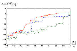
(c) Pajek network GD99c

Figure 5: In this figure we compare (in a logarithmic scale) the smallest eigenvalue of the controllability Gramian for different choices of the set of control nodes. The set of control nodes $\mathcal{K}$ is selected according to Algorithm 1 (solid red), trace optimization as in Appendix (dashed green), and randomly (dashed-dot blue). The cardinality of the control set varies from $1$ to $n$. Our decoupled control law algorithm outperforms the two counterparts, while being amenable to distributed implementation as discussed in Section IV-A.

Social network Inspired by the seminal work [42], the opinion dynamics of a group of individuals forming a network $\mathcal{G}=(\mathcal{V},\mathcal{E})$ can be modeled by the consensus system

$$x(t+1)=Ax(t),$$

where $x:\mathbb{N}\rightarrow\mathbb{R}$ is the vector of the individual opinions, and the matrix $A=[a_{ij}]$ is row stochastic and satisfies $a_{ij}=0$ whenever the edge $(i,j)$ is not in the edge set $\mathcal{E}$. Besides the description of opinion dynamics, consensus models have found broad applicability in several domains [43].

For our numerical study we consider the social network describing the Klavzar bibliography (see Fig. 4(b)), and we construct a consensus system by assigning a random nonzero weight to each edge in the network. The results of this numerical study are in Fig. 5(b).

Remark 4

(Controllability of consensus networks) Connected consensus networks feature a simple unit eigenvalue [43], so that the controllability Gramian is not defined for the infinite control horizon, as the series $\sum_{\tau=0}^{\infty}A^{\tau}B_{\mathcal{K}}B_{\mathcal{K}}^{\mathsf{T}}(A^{\mathsf{T}})^{\tau}$ is not convergent. On the other hand, it can be shown that the unit eigenvalue is controllable at $T=\infty$ by any nonempty set of control nodes with zero energy. Then, without loss of generality, the infinite horizon controllability Gramian of consensus networks can be defined by restricting the dynamics to the subspace orthogonal to the consensus space, where the matrix $A$ is Schur stable. $\square$

Epidemics spreading The N-intertwined SIS model for the dynamics of a viral infection over a network with $n$ nodes and adjacency matrix $A=[a_{ij}]$ reads as [44]

$$\dot{p}_{i}=-\alpha_{i}p_{i}+(1-p_{i})\beta_{i}\sum_{j\in\mathcal{N}_{i}}a_{ij}p_{j},\;i\in\{1,\dots,n\},$$

where $p_{i}:\mathbb{R}_{\geq 0}\rightarrow\mathbb{R}_{[0,1]}$ is the map describing the infection probability of node $i$, and $\alpha_{i}\in\mathbb{R}_{\geq 0}$, $\beta_{i}\in\mathbb{R}_{\geq 0}$ are the curing and infection rates of the $i$-th node. It is known that, for certain values of the ratios $\alpha_{i}/\beta_{i}$, an initial infection $p(0)$ may spread to all the nodes in the network or converge to zero. We consider the simplified model

$$\dot{p}_{i}=-\alpha_{i}p_{i}+\beta_{i}\sum_{j\in\mathcal{N}_{i}}a_{ij}p_{j},$$ (19)

which is a good approximation of the N-intertwined SIS model at the initial phase of the epidemics spreading when $p_{i}$ is small. We discretize the system (19) as

$$p_{i}(t+1)=(1-h\alpha_{i})p_{i}(t)+h\beta_{i}\sum_{j\in\mathcal{N}_{i}}a_{ij}p_{j}(t),$$ (20)

where $h\in\mathbb{R}_{>0}$ is a sufficiently small discretization parameter, and we study the problem of controlling the spreading of the infection throughout the network. Notice that an infection can be controlled for instance by distributing vaccines.

For our numerical study we consider the Pajek social network GD99c (see Fig. 4(c)), we let $h=10^{-2}$, and we select the parameters $\alpha_{i}$ and $\beta_{i}$ randomly so that the network (20) is unstable. Due to the instability of the network, we select a finite control horizon of $n/2$ control steps. The results of this numerical study are in Fig. 5(c).

From our numerical analysis we draw the following conclusions. First, the smallest eigenvalue of the controllability Gramian increases abruptly when the number of control nodes overcomes a certain threshold, or, equivalently, the control energy decreases abruptly when the number of control nodes overcomes a certain threshold. This phenomena is aligned with the numerical controllability transition identified in [16] via numerical simulation. Second, our decoupled control law outperforms the control strategies dictated by the optimization of the trace of the controllability Gramian and by random positioning of the control nodes, while allowing for a distributed and local implementation of the control law. The difference between the three compared strategies becomes more evident when the number of control nodes is large. Third and finally, since our decoupled control law relies on network partitioning, and computations are performed only on the obtained subnetworks, it is scalable with the network cardinality and thus suitable for application to large networks.

We conclude this section with the following consideration. In Algorithm 1 we partition each subnetwork by computing its Fiedler eigenvector. For large networks, this partitioning scheme may be inefficient, and it may be replaced by a partitioning scheme with linear complexity, such as the Louvain method [45, 46]. In this case, our method to control complex networks has linear complexity, since the decoupled control law requires only the inversion of local controllability Gramians whose dimension is independent of the network cardinality. On the other hand, assuming that the Gauss-Jordan elimination algorithm is used for the inversion of the controllability Gramian [47], the computational complexity of the minimum energy control law (4) grows at least cubically with the network cardinality.

VI Conclusion

In this work we study the problem of controlling complex networks to a target state. We adopt the smallest eigenvalue of the controllability Gramian as measure of network controllability, which quantifies the worst-case control energy. We characterize tradeoffs between the number of control nodes and the control energy as a function of the network dynamics. We develop a control strategy with performance guarantees, consisting of a method to select control nodes based on network partitioning, and a distributed control law to reach the target state. Finally, we validate our findings with power systems, social networks, and epidemics spreading examples.

Important aspects requiring further investigation include (i) the derivation of tighter bounds for the tradeoff between the number of control nodes and the control energy, as a function of network properties, (ii) the study of different controllability measures, possibly capturing the distributed nature of the problem, and (iii) the design of an efficient partitioning method to optimize the performance of our decoupled control law, and (iv) the extension of our bounds to the design of optimal $\mathcal{H}_{2}$ feedback controllers.

APPENDIX

In this section we derive a closed-form solution to the problem of selecting control nodes to maximize the trace of the controllability Gramian, as considered for instance in [17]. To simplify notation we focus on symmetric networks, although analogous results hold for asymmetric networks. Specifically, we consider the maximization problem

$$\begin{split}&\max_{\mathcal{K}\subseteq\{1,\dots,n\}}\text{Trace}(\mathcal{W}_{\mathcal{K},T}),\\ &\text{subject to}\;\;\;|\mathcal{K}|=m,\end{split}$$ (A-1)

where $m\leq n$ and $T\in\mathbb{N}_{\geq 1}$. Notice that

$$\text{Tr}(\mathcal{W}_{\mathcal{K},T}) =\text{Tr}\left(\sum_{\tau=0}^{T-1}A^{\tau}B_{\mathcal{K}}B_{\mathcal{K}}^{\mathsf{T}}A^{\tau}\right)=\sum_{\tau=0}^{T-1}\text{Tr}\left(B_{\mathcal{K}}B_{\mathcal{K}}^{\mathsf{T}}A^{2\tau}\right)$$

$$=\text{Tr}\left(B_{\mathcal{K}}B_{\mathcal{K}}^{\mathsf{T}}\sum_{\tau=0}^{T-1}A^{2\tau}\right)=\sum_{i\in\mathcal{K}}\left(\sum_{\tau=0}^{T-1}A^{2\tau}\right)_{ii},$$

where we have used that trace is a linear map and is invariant under cyclic permutations [20], and where $\left(\sum_{\tau=0}^{T-1}A^{2\tau}\right)_{ii}$ denotes the $i$-th diagonal entry of the matrix $\sum_{\tau=0}^{T-1}A^{2\tau}$. We conclude that a solution to the maximization problem (A-1) is the set $\mathcal{K}^{*}$ containing the indices of the $m$ largest diagonal entries of $\left(\sum_{\tau=0}^{T-1}A^{2\tau}\right)$. Notice that, if $A$ is Schur stable, then $\sum_{\tau=0}^{\infty}A^{2\tau}=(I-A^{2})^{-1}$.

References

- [1] T. Kailath, Linear Systems. Prentice-Hall, 1980.
- [2] R. E. Kalman, Y. C. Ho, and S. K. Narendra, “Controllability of linear dynamical systems,” Contributions to Differential Equations, vol. 1, no. 2, pp. 189–213, 1963.
- [3] R. W. Brockett, Finite Dimensional Linear Systems. Wiley and Sons, 1970.
- [4] K. J. Reinschke, Multivariable Control: A Graph-Theoretic Approach. Springer, 1988.
- [5] Y. Y. Liu, J. J. Slotine, and A. L. Barabási, “Controllability of complex networks,” Nature, vol. 473, no. 7346, pp. 167–173, 2011.
- [6] Y.-Y. Liu, J.-J. Slotine, and A.-L. Barabási, “Observability of complex systems,” Proceedings of the National Academy of Sciences, vol. 110, no. 7, pp. 2460–2465, 2013.
- [7] W. M. Wonham, Linear Multivariable Control: A Geometric Approach, 3rd ed. Springer, 1985.
- [8] G. Parlangeli and G. Notarstefano, “On the reachability and observability of path and cycle graphs,” IEEE Transactions on Automatic Control, vol. 57, no. 3, pp. 743–748, 2012.
- [9] J. M. Dion, C. Commault, and J. van der Woude, “Generic properties and control of linear structured systems: a survey,” Automatica, vol. 39, no. 7, pp. 1125–1144, 2003.
- [10] F.-J. Müller and A. Sachuppert, “Few inputs can reprogram biological networks,” Nature, vol. 478, no. 7369, pp. E4–E4, 2011.
- [11] N. J. Cowan, E. J. Chastain, D. A. Vilhena, J. S. Freudenberg, and C. T. Bergstrom, “Nodal dynamics, not degree distributions, determine the structural controllability of complex networks,” PLOS ONE, vol. 7, no. 6, p. e38398, 2012.
- [12] A. Rahmani, M. Ji, M. Mesbahi, and M. Egerstedt, “Controllability of multi-agent systems from a graph-theoretic perspective,” SIAM Journal on Control and Optimization, vol. 48, no. 1, pp. 162–186, 2009.
- [13] A. Olshevsky, “The minimal controllability problem,” 2013, arXiv preprint arXiv:1304.3071.
- [14] G. Notarstefano and G. Parlangeli, “Controllability and observability of grid graphs via reduction and symmetries,” IEEE Transactions on Automatic Control, vol. 58, no. 7, pp. 1719–1731, 2013.
- [15] G. Yan, J. Ren, Y.-C. Lai, C.-H. Lai, and B. Li, “Controlling complex networks: How much energy is needed?” Physical Review Letters, vol. 108, no. 21, p. 218703, 2012.
- [16] J. Sun and A. E. Motter, “Controllability transition and nonlocality in network control,” Physical Review Letters, vol. 110, no. 20, p. 208701, 2013.
- [17] T. H. Summers and J. Lygeros, “Optimal sensor and actuator placement in complex dynamical networks,” 2013, arXiv preprint arXiv:1306.2491.
- [18] A. Chapman and M. Mesbahi, “System theoretic aspects of influenced consensus: Single input case,” IEEE Transactions on Automatic Control, vol. 57, no. 6, pp. 1505–1511, 2012.
- [19] A. C. Antoulas, D. C. Sorensen, and Y. Zhou, “On the decay rate of Hankel singular values and related issues,” Systems & Control Letters, vol. 46, no. 5, pp. 323–342, 2002.
- [20] R. A. Horn and C. R. Johnson, Matrix Analysis. Cambridge University Press, 1985.
- [21] A. M. A. Hamdan and A. H. Nayfeh, “Measures of modal controllability and observability for first-and second-order linear systems,” AIAA Journal of Guidance, Control, and Dynamics, vol. 12, no. 3, pp. 421–428, 1989.
- [22] I. Rajapakse, M. Groudine, and M. Mesbahi, “Dynamics and control of state-dependent networks for probing genomic organization,” Proceedings of the National Academy of Sciences, vol. 108, no. 42, pp. 17 257–17 262, 2011.
- [23] P. C. Müller and H. I. Weber, “Analysis and optimization of certain qualities of controllability and observability for linear dynamical systems,” Automatica, vol. 8, no. 3, pp. 237–246, 1972.
- [24] M. Van De Wal and B. De Jager, “A review of methods for input/output selection,” Automatica, vol. 37, no. 4, pp. 487–510, 2001.
- [25] P. L. Sharon and K. K. Rex, “Optimization strategies for sensor and actuator placement,” NASA Langley Technical Report, Tech. Rep., 1999.
- [26] B. Marx, D. Koenig, and D. Georges, “Optimal sensor and actuator location for descriptor systems using generalized Gramians and balanced realizations,” in American Control Conference, Boston, MA, USA, July 2004, pp. 2729–2734.
- [27] H. R. Shaker and M. Tahavori, “Optimal sensor and actuator location for unstable systems,” Journal of Vibration and Control, 2012. [Online]. Available: http://jvc.sagepub.com/cgi/content/abstract/1077546312451302v1
- [28] F. L. Bauer and C. Fike, “Norms and exclusion theorems,” Numerische Mathematik, vol. 2, no. 1, pp. 137–141, 1960.
- [29] S. Boyd, A. Ghosh, B. Prabhakar, and D. Shah, “Randomized gossip algorithms,” IEEE Transactions on Information Theory, vol. 52, no. 6, pp. 2508–2530, 2006.
- [30] D. Georges, “The use of observability and controllability Gramians or functions for optimal sensor and actuator location in finite-dimensional systems,” in IEEE Conf. on Decision and Control, New Orleans, LA, USA, Dec. 1995, pp. 3319–3324.
- [31] S. S. Rao, T.-S. Pan, and V. B. Venkayya, “Optimal placement of actuators in actively controlled structures using genetic algorithms,” AIAA Journal, vol. 29, no. 6, pp. 942–943, 1991.
- [32] K. B. Lim, “Method for optimal actuator and sensor placement for large flexible structures,” AIAA Journal of Guidance, Control, and Dynamics, vol. 15, no. 1, pp. 49–57, 1992.
- [33] S. Fortunato, “Community detection in graphs,” Physics Reports, vol. 486, no. 3-5, pp. 75–174, 2010.
- [34] S. Skogestad and I. Postlethwaite, Multivariable Feedback Control Analysis and Design, 2nd ed. Wiley, 2005.
- [35] W. H. Kwon, Y. S. Moon, and S. C. Ahn, “Bounds in algebraic Riccati and Lyapunov equations: a survey and some new results,” International Journal of Control, vol. 64, no. 3, pp. 377–389, 1996.
- [36] M. E. J. Newman, Networks: An Introduction. Oxford University Press, 2010.
- [37] M. Fiedler, “Algebraic connectivity of graphs,” Czechoslovak Mathematical Journal, vol. 23, no. 2, pp. 298–305, 1973.
- [38] P. Kundur, Power System Stability and Control. McGraw-Hill, 1994.
- [39] F. Dörfler and F. Bullo, “Synchronization and transient stability in power networks and non-uniform Kuramoto oscillators,” SIAM Journal on Control and Optimization, vol. 50, no. 3, pp. 1616–1642, 2012.
- [40] R. D. Zimmerman, C. E. Murillo-Sánchez, and D. Gan, “MATPOWER: Steady-state operations, planning, and analysis tools for power systems research and education,” IEEE Transactions on Power Systems, vol. 26, no. 1, pp. 12–19, 2011.
- [41] Y. Hu, “Efficient, high-quality force-directed graph drawing,” Mathematica Journal, vol. 10, no. 1, pp. 37–71, 2005.
- [42] M. H. DeGroot, “Reaching a consensus,” Journal of the American Statistical Association, vol. 69, no. 345, pp. 118–121, 1974.
- [43] F. Garin and L. Schenato, “A survey on distributed estimation and control applications using linear consensus algorithms,” in Networked Control Systems, ser. LNCIS, A. Bemporad, M. Heemels, and M. Johansson, Eds. Springer, 2010, pp. 75–107.
- [44] P. V. Mieghem, J. Omic, and R. Kooij, “Virus spread in networks,” IEEE/ACM Transactions on Networking, vol. 17, no. 1, pp. 1–14, 2009.
- [45] V. D. Blondel, J.-L. Guillaume, R. Lambiotte, and E. Lefebvre, “Fast unfolding of communities in large networks,” Journal of Statistical Mechanics: Theory and Experiment, vol. 2008, no. 10, p. P10008, 2008.
- [46] J.-C. Delvenne, S. N. Yaliraki, and M. Barahona, “Stability of graph communities across time scales,” Proceedings of the National Academy of Sciences, vol. 107, no. 29, pp. 12 755–12 760, 2010.
- [47] V. Strassen, “Gaussian elimination is not optimal,” Numerische Mathematik, vol. 13, no. 4, pp. 354–356, 1969.