Nonautonomous control of stable and unstable manifolds in two-dimensional flows

Abstract

We outline a method for controlling the location of stable and unstable manifolds in the following sense. From a known location of the stable and unstable manifolds in a steady two-dimensional flow, the primary segments of the manifolds are to be moved to a user-specified time-varying location which is near the steady location. We determine the nonautonomous perturbation to the vector field required to achieve this control, and give a theoretical bound for the error in the manifolds resulting from applying this control. The efficacy of the control strategy is illustrated via a numerical example.

1 Introduction

The role of stable and unstable manifolds in demarcating flow barriers in unsteady flows is well documented. Determining their location in a given unsteady flow regime is a problem which has attracted considerable attention, with many techniques continually being developed and refined in order to improve accuracy and efficiency [1, 2, 3, 4, 5, 6, 7, 8, 9, 10, 11, 12, 13, 14, 15, 16, 17, 18, 19].

Viewing this problem from the reverse viewpoint leads to an intriguing question: is it possible to force stable and unstable manifolds to lie along user-defined, time-varying locations? The time-variation here is arbitrarily specified, and not confined to the popular time-periodic situation. If possible, this would yield an invaluable tool in controlling transport in micro- and nano-fluidic devices, with innumerable applications. This article answers this question in a specific setting: that of a nonautonomously perturbed two-dimensional system, in which the issue is to determine the nonautonomous perturbation which gives rise to the primary parts of the stable and unstable manifolds lying along prescribed one-dimensional curves at each instance in time. The theory is couched in terms of the perturbation being ${\mathcal{O}}(\varepsilon)$, and results ensuring that the prescribed manifolds are achieved to leading-order in $\varepsilon$ are presented. Rigorous bounds for the errors in the manifolds are also established.

The derived control strategy is tested on a time-aperiodic modification of the Taylor-Green flow [20, 21, 22, 23, 24]. Numerical diagnostics are compared with the prescribed stable manifolds, and excellent results are obtained.

While the method developed in this article is confined to perturbations of autonomous flows, it is to our knowledge the first theoretical contribution towards developing a control strategy for stable and unstable manifolds in nonautonomous flows. As such, it may serve as an important initial step towards building a more complete theory for the nonautonomous control of flow barriers.

2 Controlling stable manifold

Consider for $x\in\Omega$, a two-dimensional open connected set, the system

$$\dot{x}=f(x)$$ (1)

in which $f:\Omega\rightarrow{\mathbb{R}}^{2}$, and sufficient smoothness will be assumed (to be characterised shortly).

Hypothesis 2.1 (Saddle point at $a$)

The system (1) possesses a saddle fixed point $a$, that is, $f(a)=0$ and $Df(a)$ possesses real eigenvalues $\lambda_{s}$ and $\lambda_{u}$ such that $\lambda_{s}<0<\lambda_{u}$.

Then, $a$ possesses corresponding one-dimensional stable and unstable manifolds. We will focus on segments of one branch of each of these manifolds, and denote them by $\Gamma_{s}$ and $\Gamma_{u}$ respectively. The segment of the stable manifold branch we will consider can be represented parametrically by

$$\Gamma_{s}:=\left\{x_{s}(p)~{}:~{}p\in[S,\infty)\right\}$$

in which $x_{s}(t)$ is a solution to (1) with initial condition $x_{s}(0)\in\Gamma_{s}$, and $S\in\left(-\infty,0\right]$ represents a finite backwards time until which the trajectory is evolved. Notice in particular that $x_{u}(t)\rightarrow a$ as $t\rightarrow\infty$, and so $\bar{\Gamma}_{s}$ contains $a$, while the other end of the curve segment comprising $\Gamma_{s}$ ends at the point $x_{s}(S)$. From this definition, it is clear that $\Gamma_{s}$ cannot be (i) a branch of a stable manifold which has infinite length, or (ii) a heteroclinic or homoclinic manifold associated with a fixed point since $x_{s}(t)$ cannot approach a fixed point in finite time. On the other hand, $\Gamma_{s}$ could be any other finite length restriction of a branch of the stable manifold emanating from $a$, including a segment of any of the above two entities, or a segment of a manifold which has many rotations as it spirals out from a limit cycle. Similarly, let $\Gamma_{u}$ be a restricted branch of the unstable manifold of $a$ which is parametrisable as

$$\Gamma_{u}:=\left\{x_{u}(p)~{}:~{}p\in(-\infty,U]\right\}$$

in which $x_{u}(t)$ is a solution to (1) with initial condition $x_{u}(0)\in\Gamma_{u}$, and which satisfies $x_{u}(t)\rightarrow a$ as $t\rightarrow-\infty$, and $U\in[0,\infty)$ is a finite forward time until which the trajectory is evolved. See Fig. 1 for an example of the finite segments $\Gamma_{s}$ and $\Gamma_{u}$.

Figure 1: The restricted stable manifold $\Gamma_{s}$ (thick blue curve) and unstable manifold $\Gamma_{u}$ (thick red curve) of the fixed point $a$, in the situation in which the stable manifold exhibits spiralling and the unstable manifold escapes to infinity.

The goal is to determine a nonautonomous perturbation to the vector field in the form

$$\dot{x}=f(x)+\varepsilon g(x,t)$$ (2)

in which $\varepsilon\in[0,\varepsilon_{0})$ where $\varepsilon_{0}\ll 1$, such that $\Gamma_{s}$ and $\Gamma_{u}$ perturb to $\varepsilon$-close time-dependent entities which are specified. The following smoothness hypotheses on the functions $f$ and $g$ will be assumed, in which $D$ represents the spatial (matrix) derivative operator in $\Omega$.

Hypothesis 2.2 (Smoothness of $f$ and $g$)

The functions $f:\Omega\rightarrow{\mathbb{R}}^{2}$ and $g:\Omega\times{\mathbb{R}}\rightarrow{\mathbb{R}}^{2}$ satisfy the following smoothness and boundedness assumptions.

• $f\in{\mathrm{C}}^{2}\left(\Omega\right)$, and is such that there exists a constant $C_{f}$ satisfying

  $$\left\|f\left(x\right)\right\|+\left\|Df\left(x\right)\right\|+\left\|D^{2}f\left(x\right)\right\|\leq C_{f}~{}~{}{\mathrm{for~{}all}}~{}x\in\Omega\,.$$ (3)

• $g\in{\mathrm{C}}^{2}\left(\Omega\right)$ for each $t\in{\mathbb{R}}$, and $g\in{\mathrm{C}}^{1}\left({\mathbb{R}}\right)$ for each $x\in\Omega$, and moreover there exists a constant $C_{g}$ satisfying

  $$\left\|g\left(x,t\right)\right\|+\left\|Dg\left(x,t\right)\right\|+\left\|\frac{\partial g}{\partial t}\left(x,t\right)\right\|\leq C_{g}~{}~{}{\mathrm{for~{}all}}~{}(x,t)\in\Omega\times{\mathbb{R}}\,.$$ (4)

A note on the norms used in (3) and (4) is in order. The norm on ${\mathbb{R}}^{2}$ is the standard Euclidean norm; we could have stated the relevant norms on $f$, $g$ and $\partial g/\partial t$ by using the modulus $\left|\centerdot\right|$ instead. The norm on the $2\times 2$ matrices $Df$ and $Dg$ is the operator norm induced by the Euclidean norm. The norm on the $2\times 2\times 2$ entity $D^{2}f$ is the induced operator norm associated with the above norms on vectors and matrices, i.e.,

$$\left\|\left(D^{2}f\right)\right\|=\sup_{v\in{\mathbb{R}}^{2}\setminus 0}\frac{\left\|\left(D^{2}f\right)\,v\right\|}{\left\|v\right\|}\,,$$ (5)

in which the previously mentioned operator norm definition for $2\times 2$ matrices is used in the numerator.

Now, the smooth function $g(x,t)$ will be the control which achieves the desired stable and unstable manifolds, which can be now represented by $\Gamma_{s}^{\varepsilon}(t)$ and $\Gamma_{u}^{\varepsilon}(t)$ respectively. In viewing these restrictions to the manifolds in this nonautonomous setting, it makes sense to represent (2) in the augmented form

$$\left.\begin{array}[]{l}\dot{x}=f(x)+\varepsilon g(x,t)\\ \dot{t}=1\end{array}\right\}\,$$ (6)

with phase space now being $\Omega\times{\mathbb{R}}$. For (6) when $\varepsilon=0$, the conditions stated for (1) provide for the presence of a hyperbolic trajectory $\left(a,t\right)$ with two-dimensional stable and unstable manifolds.

From this point onwards, this Section will focus only on controlling the stable manifold, with the unstable manifold control description postponed to the subsequent Section. It will be necessary to restrict the stable manifold in time in the following sense. Let $T_{s}<0$ be a time-value beyond which the restricted stable manifold is to be defined. This signs for $T_{s}$ is chosen to ensure that $t=0$ is a legitimate choice for both the restricted stable and unstable manifolds. Restricting time in this way will be necessary when $\varepsilon\neq 0$ because the restrictions on $p$ mean that only segments of the relevant manifolds are defined in each time-slice, and since these segments evolve with time further restrictions will arise. The restricted two-dimensional stable manifold of (6) when $\varepsilon=0$ will be represented in parametric form by

$$\Gamma_{s}:=\left\{\left(x_{s}(t-T_{s}+p),t\right)~{}:~{}(p,t)\in[S,\infty)\times[T_{s},\infty)\right\}\,,$$ (7)

in which the notation $\Gamma_{s}$ is retained with an abuse of notation. This parametrisation with respect to $(p,t)$ has been chosen such that the parameter $p$ selects the specific trajectory on the relevant manifold of (6) when $\varepsilon=0$, and $t$ represents the time-evolution of that trajectory. So for example if a point $x_{s}(p)$ is chosen in the time-slice $t=T_{s}$, then $\left(x_{s}(t-T_{s}+p),t\right)$ represents the corresponding forward trajectory on $\Gamma_{s}$ as it evolves with time $t$. In the time-slice $T_{s}$, the restriction $p\geq S$ implies the relevant segment of the unperturbed stable manifold goes from $x_{s}(S)$ to $a$. Now, in a time-slice $t>T_{s}$, the trajectory through $x_{s}(S)$ would have evolved to the location $x_{s}(S+t-T_{s})$, and information on $x_{s}(p)$ for $p$ values less than $S+t-T_{s}$ cannot be available since such would correspond to points on the stable manifold which were beyond $x_{s}(S)$ at time $T_{s}$. As time $t$ evolves for the unperturbed steady flow (1), $x_{s}(S+t-T_{s})$ approaches the saddle fixed point $a$, and therefore the length of the restricted stable manifold in each time-slice gets shorter. In other words, the restrictions implied in (7) results are actually associated with shorter and shorter segments of the stable manifold as time gets larger. This is illustrated in Fig. 2, in which trajectories associated with five $p$ values are shown beginning with an “initial” point in the time-slice $T_{s}$. The “furthest” of these corresponds to the initial point $x_{s}(S)$ (i.e., $p=S$), and after three intermediate $p$ values, the dashed trajectory is $(a,t)$, which can be thought of as $p=\infty$ in (7). The stable manifold in the time-slice $T_{s}$ is the curve segment (heavy magenta curve) which connects together all five starting points. In time-slices $t$ as time evolves, all trajectories get closer together (indeed, they get closer to the dashed hyperbolic trajectory $(a,t)$), which means that the restricted stable manifold are becoming curves of smaller and smaller length in each time-slice. These are indicated at two later time values in Fig. 2, also as heavy magenta curves. A similar description works for the restricted unstable manifolds in (7), but in this case the manifold segments in each time-slice becomes shorter curves as $t$ decreases.

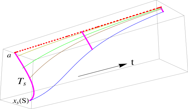
Figure 2: The evolution of the restricted stable manifold curve (heavy magenta curves), and the hyperbolic trajectory (dashed red line).

Now, when $\varepsilon\neq 0$, and for any $g$ satisfying the smoothness assumptions in Hypothesis 2.2, the hyperbolic trajectory $\left(a,t\right)$ of (6) perturbs to an ${\mathcal{O}}(\varepsilon)$-close trajectory $\left(a_{\varepsilon}(t),t\right)$ which retains hyperbolicity. The proof of this is via exponential dichotomies [25, 26, 27], and as a consequence this trajectory retains stable and unstable manifolds which are $\varepsilon$-close to the original ones. In particular, it retains a stable manifold $\varepsilon$-close to (7). The locations of the manifold will depend on the choice of $g$, but here we specify the perturbed restricted manifolds, and find additional conditions on $g$ in order to achieve these. The desired restricted stable manifold will be represented parametrically by

$$\Gamma_{s}^{\varepsilon}:=\left\{\left(x_{s}^{\varepsilon}(p,t),t\right)~{}:~{}(p,t)\in[S,\infty)\times[T_{s},\infty)\right\}\,,$$ (8)

where the parametrisation $x_{s}^{\varepsilon}$ is assumed given, but satisfies several conditions to ensure consistency. To express these conditions, we first define

$$J=\left(\begin{array}[]{lr}0&-1\\ 1&0\end{array}\right)\,,$$ (9)

the premultiplicative matrix which rotates vectors in ${\mathbb{R}}^{2}$ by $+\pi/2$.

Hypothesis 2.3 (Stable manifold requirements)

For each $t\geq T_{s}$, the quantity $\left\{x_{s}^{\varepsilon}(p,t)~{}:~{}p\geq S\right\}$ is a curve in $\Omega$. These restricted stable manifold curves satisfy the following conditions.

• [Smoothness] There exists a constant $K_{s}>0$ such that for all $(p,t)\in[S,\infty)\times[T_{s},\infty)$ and for all $\varepsilon\in(0,\varepsilon_{0})$,

  $$\left|x_{s}^{\varepsilon}(p,t)\right|+\left|\frac{\partial}{\partial t}x_{s}^{\varepsilon}(p,t)\right|+\left|\frac{\partial}{\partial p}x_{s}^{\varepsilon}(p,t)\right|+\left|\frac{\partial}{\partial\varepsilon}x_{s}^{\varepsilon}(p,t)\right|+\left|\frac{\partial^{2}}{\partial\varepsilon^{2}}x_{s}^{\varepsilon}(p,t)\right|+\left|\frac{\partial^{3}}{\partial\varepsilon^{3}}x_{s}^{\varepsilon}(p,t)\right|<K_{s}\,.$$ (10)

• [Closeness] There exists a constant $C_{s}>0$ such that for all $(p,t)\in[S,\infty)\times[T_{s},\infty)$,

  $$\left|x_{s}^{\varepsilon}(p,t)-x_{s}(t-T_{s}+p)\right|+\left|\frac{\partial}{\partial p}\left(x_{s}^{\varepsilon}(p,t)-x_{s}(t-T_{s}+p)\right)\right|\leq C_{s}\,\varepsilon\,.$$ (11)

• [Limit] For each $t\geq T_{s}$, $\displaystyle\lim_{p\rightarrow\infty}x_{s}^{\varepsilon}(p,t)$ is well defined.

• [Mappability] For each $t\geq T_{s}$, there exist intervals $\left[S_{1}(t),S_{2}(t)\right)$ and $\left[S_{1}^{\varepsilon}(t),S_{2}^{\varepsilon}(t)\right)$ —both of which are contained in $[S,\infty)$— and a scalar function $r_{s}(\centerdot,t)$ defined on $\left[S_{1}(t),S_{2}(t)\right)$ which satisfies

  $$x_{s}^{\varepsilon}(p^{\varepsilon},t)=x_{s}(t-T_{s}+p)+r_{s}(p,t)\frac{Jf\left(x_{s}(t-T_{s}+p)\right)}{\left|Jf\left(x_{s}(t-T_{s}+p)\right)\right|}\,,$$ (12)

  such that the mapping $p\rightarrow p^{\varepsilon}$ from $\left[S_{1}(t),S_{2}(t)\right)$ to $\left[S_{1}^{\varepsilon}(t),S_{2}^{\varepsilon}(t)\right)$ defined through (12) is a diffeomorphism.

• [Congruence at time zero] The $p$ parameters in the time-slice $t=0$ between the unperturbed and the required restricted stable manifold curves match up, i.e., for all $p\in\left[S_{1}(0),S_{2}(0)\right)$,

  $$\left[f\left(x_{s}(-T_{s}+p)\right)\right]^{T}\left[x_{s}^{\varepsilon}(p,0)-x_{s}(-T_{s}+p)\right]=0\,.$$ (13)

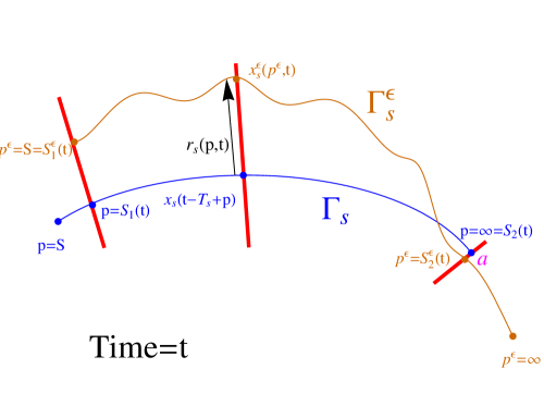
Figure 3: An illustration of the mappability condition (12) in the time-slice $t$. The heavy lines are in the normal direction $Jf$ to $\Gamma_{s}$. The interval $\left[S_{1}(t),S_{2}(t)\right)$ is the $p$-interval for which the it is possible to map from $\Gamma_{s}$ to $\Gamma_{s}^{\varepsilon}$ by going in the normal direction $\Gamma_{s}$, while $\left[S_{1}^{\varepsilon}(t),S_{2}^{\varepsilon}(t)\right)$ is the corresponding interval for $p^{\varepsilon}$ which parametrises $\Gamma_{s}^{\varepsilon}$. In this pictured situation, $S_{2}(t)=\infty$ and $S_{1}^{\varepsilon}(t)=S$.

These hypotheses require some explanation. The condition (10) is a straightforward requirements on the smoothness and boundedness of the required restricted manifold. The condition (11) is a ${\mathcal{O}}(\varepsilon)$-closeness requirements between $x_{s}^{\varepsilon}(p,t)$ and $x_{s}(t-T_{s}+p)$ at each $(p,t)$ value. In particular, for each fixed $t\in[T_{s},\infty)$, the curves $x_{s}^{\varepsilon}(p,t)$ and $x_{s}(t-T_{s}+p)$ and their tangents in the $t$ time-slice are assumed to remain $\varepsilon$-close. Condition (c) requires that the end of the curve – that purportedly is on the hyperbolic trajectory $a_{\varepsilon}(t)$ – is well-defined. While becoming unbounded is already precluded by condition (a), condition (c) prevents $x_{s}^{\varepsilon}(p,t)$ behaving like, say, $\cos p$ for large $p$.

The condition in Hypothesis 2.3(d) prevents for example choosing $x_{s}^{\varepsilon}(p,t)$ such that a self-intersecting curve is generated in a time-slice. The intuition is that in each time slice $t$ the restricted autonomous stable manifold segment and the required restricted nonautonomous stable manifold segment are mappable to one another by proceeding in the normal direction to each point $x_{s}(t-T_{s}-p)$, by a signed distance $r_{s}(p,t)$. The restriction of $p$ and $p^{\varepsilon}$ to these subintervals of $[S,\infty)$ is since some parts of the required $\Gamma_{s}^{\varepsilon}$ may venture “beyond” the span of the normal direction to $\left\{x_{s}(t-T_{s}+p)~{};~{}p\in[S,\infty)\right\}$. This condition is illustrated by example in Fig. 3. This mapping from $\Gamma_{s}$ to $\Gamma_{s}^{\varepsilon}$ by going along the normal direction $Jf$ from each point on $\Gamma_{s}$ parametrised by $p$ must be a diffeomorphism from $\left[S_{1}(t),S_{2}(t)\right)$ to $\left[S_{1}^{\varepsilon}(t),S_{2}^{\varepsilon}(t)\right)$, which prevents $\Gamma_{s}^{\varepsilon}$ having self-intersections or twists which make the inverse function undefined.

Finally, the congruence condition (e) reflects a choice of parametrisation taken in the time-slice $t=0$, which is shown in Fig. 4 for the restricted stable manifold. For any fixed $p$, consider the point $x_{s}(-T_{s}+p)$ on the unperturbed stable manifold, and suppose we draw a line perpendicular to $f\left(x_{s}(-T_{s}+p)\right)$ in this time-slice $t=0$, as shown in Fig. 4. Now, the intersections of $\Gamma_{s}^{\varepsilon}$ and $\tilde{\Gamma}_{s}^{\varepsilon}$ in the time-slice $0$ are also shown in this figure, and the normal line intersects each of these curves. The congruence condition (13) in the time-slice $t=0$ means that the $p$-parametrisation of $x_{s}^{\varepsilon}(p,0)$ is chosen such that $x_{s}^{\varepsilon}(p,0)$ lies exactly on this normal line drawn at $x_{s}(-T_{s}+p)$. We have the freedom to do this for all mappable $p$ in this one particular time-slice; it is merely a choice of parametrisation of the one dimensional curve obtained by intersecting $\Gamma_{s}^{\varepsilon}$ with the time-slice $\left\{t=0\right\}$.

Figure 4: The congruence condition (13) in the time-slice $t=0$: at each $p$, the normal vector at $x_{s}(-T_{s}+p)$ meets $\Gamma_{s}^{\varepsilon}$ at the point $x_{s}^{\varepsilon}(p,0)$.

Figure 5: The congruence conditions (13) and (21) in the time-slice $t=0$, illustrating that both the required ($\Gamma_{s}^{\varepsilon}$) and the real ($\tilde{\Gamma}_{s}^{\varepsilon}$) stable manifolds have a congruent $p$-paramatrisation at time zero.

While the desired restricted stable manifold is given by (8), Hypotheses 2.3 further restricts the $(p,t)$ values to lie in the set

$$\Xi_{s}:=\left\{\left(p,t\right)~{}:~{}t\geq T_{s}~{}{\mathrm{and}}~{}S_{1}(t)\leq p<S_{2}(t)\right\}\,.$$ (14)

We will assume that the largest interval $\left[S_{1}(t),S_{2}(t)\right)$ has been chosen for each $t$ in order to fulfil the mappability condition of Hypothesis 2.3.

For $(p,t,\varepsilon)\in\Xi_{s}\times(0,\varepsilon_{0})$, we define

$$M_{s}^{\varepsilon}(p,t):=\left[Jf\left(x_{s}(t-T_{s}+p)\right)\right]^{T}\frac{x_{s}^{\varepsilon}(p,t)-x_{s}(t-T_{s}+p)}{\varepsilon}$$ (15)

and

$$B_{s}^{\varepsilon}(p,t):=\left[f\left(x_{s}(t-T_{s}+p)\right)\right]^{T}\frac{x_{s}^{\varepsilon}(p,t)-x_{s}(t-T_{s}+p)}{\varepsilon}\,,$$ (16)

which respectively represent projections of the difference between the unperturbed and the desired restricted stable manifold in the normal and tangential directions to the original manifold $\Gamma_{s}$ in the time-slice $t$ . Note that for a specified $x_{s}^{\varepsilon}(p,t)$, both $M_{s}^{\varepsilon}$ and $B_{s}^{\varepsilon}$ can be computed numerically based on the above expressions. Now, the required values of $g$ (to leading-order) shall be expressed in terms of an orthogonal basis formed by projecting normally and tangentially to the autonomous stable manifold at $x_{s}(t-T_{s}+p)$ in the time-slice $t$.

Definition 2.1 (Control velocity for stable manifold)

The control velocity $g$ satisfies the smoothness conditions of Hypothesis 2.2, and moreover is specified by

$$g^{\perp}\left(x_{s}(t-T_{s}+p),t\right) := \frac{\left[Jf\left(x_{s}(t-T_{s}+p)\right)\right]^{T}}{\left|f\left(x_{s}(t-T_{s}+p)\right)\right|}g\left(x_{s}(t-T_{s}+p),t\right)$$ (17)

$$= \frac{\frac{\partial M_{s}^{\varepsilon}}{\partial t}(p,t)-{\mathrm{Tr}}\,\left(Df\right)M_{s}^{\varepsilon}(p,t)}{\left|f\right|}$$

and

$$g^{\|}\left(x_{s}(t-T_{s}+p),t\right) := \frac{\left[f\left(x_{s}(t-T_{s}+p)\right)\right]^{T}}{\left|f\left(x_{s}(t-T_{s}+p)\right)\right|}g\left(x_{s}(t-T_{s}+p),t\right)$$ (18)

$$=\frac{\left|f\right|^{2}\frac{\partial B_{s}^{\varepsilon}(p,t)}{\partial t}-f^{T}\left[(Df)+(Df)^{T}\right]\left[JfM_{s}^{\varepsilon}(p,t)+fB_{s}^{\varepsilon}(p,t)\right]}{\left|f\right|^{3}}$$

in which $f$ and $Df$ in the above expressions are evaluated at $x_{s}(t-T_{s}+p)$,

By choosing $g$ as above, it will be possible to achieve the desired nonautonomous stable manifold correct to ${\mathcal{O}}(\varepsilon)$. We will in Theorem 27 specify the error precisely. First, let us describe how to apply this control velocity computationally to achieve the desired stable manifold. Suppose we are given the parametrised form $x_{s}^{\varepsilon}(p,t)$ of the restricted manifold $\Gamma_{s}^{\varepsilon}$, and full knowledge of the nearby unperturbed steady flow (1). To compute the control condition required to obtain the restricted stable manifold to leading-order, we proceed as follows.

1. Since full knowledge of the unperturbed steady flow (1) is presumed known, compute $x_{s}(p)$, and hence compute $f\left(x_{s}(t-T_{s}+p)\right)$, $Df\left(x_{s}(t-T_{s}+p)\right)$ and ${\mathrm{Tr}}\,Df\left(x_{s}(t-T_{s}+p)\right)$ as functions of $(p,t)$;

2. Since the restricted perturbed manifold $\Gamma_{s}^{\varepsilon}$ is presumed specified through its parametrisation $x_{s}^{\varepsilon}(p,t)$, compute $M_{s}^{\varepsilon}(p,t)$ and $B_{s}^{\varepsilon}(p,t)$ from (15) and (16), recalling the restriction $(p,t)\in\Xi_{s}$;

3. Determine the $t$-derivatives of both $M_{s}^{\varepsilon}(p,t)$ and $B_{s}^{\varepsilon}(p,t)$, using a numerical method if needed;

4. Substitute these values into (17) and (18) to determine $g_{s}^{\perp}$ and $g_{s}^{\|}$, where in each time-slice $t$, the values are found along the restricted part of $\Gamma_{s}$ lying between $x_{s}(t-T_{s}+S)$ and $a$;

5. Since $g^{\perp}$ and $g^{\|}$ give the components of $g$ in the directions $Jf$ and $f$ respectively, this determines $g$ at the locations $x_{s}(t-T_{s}+p)$ in time-slices $t$;

6. Extend $g$ in any suitably relevant fashion to the spatial domain while being consistent with this requirement.

To characterise the fact that this procedure results in a nonautonomous stable manifold which is correct to ${\mathcal{O}}(\varepsilon)$, and to additionally quantify the error resulting from this process, we need to compare the desired stable manifold as specified in Hypothesis 2.3 with the true stable manifold resulting from applying the control velocity of Def. 2.1. We define this true stable manifold by

$$\tilde{\Gamma}_{s}^{\varepsilon}:=\left\{\left(\tilde{x}_{s}^{\varepsilon}(p,t),t\right)~{}:~{}(p,t)\in\Xi_{s}\right\}\,,$$ (19)

rather than (8), in which the $\tilde{x}_{s}^{\varepsilon}(p,t)$ is an exact trajectory of (2) in which $g$ is as specified in Def. 2.1. For each $p$, the trajectory $\tilde{x}_{s}^{\varepsilon}(p,t)$ lies on the associated true perturbed manifold $\tilde{\Gamma}_{s}^{\varepsilon}$, with the $t$ parametrising the time evolution. Thus, $\left|\tilde{x}_{s}^{\varepsilon}(p,t)-a_{\varepsilon}(t)\right|\rightarrow 0$ as $t\rightarrow\infty$ for any $p$. Moreover, the parametrisation $p$ can be chosen so that $\tilde{x}_{s}^{\varepsilon}(p,t)$ is ${\mathcal{O}}(\varepsilon)$-close to $x_{s}(t-T_{s}+p)$, that is, there exists a constant $\tilde{C}_{s}$ such that

$$\left|\tilde{x}_{s}^{\varepsilon}(p,t)-x_{s}(t-T_{s}+p)\right|+\left|\frac{\partial}{\partial p}\left(\tilde{x}_{s}^{\varepsilon}(p,t)-x_{s}(t-T_{s}+p)\right)\right|\leq\varepsilon\tilde{C}_{s}$$ (20)

for $(p,t,\varepsilon)\in\Xi_{s}\times[0,\varepsilon_{0})$. The expectation is that $\tilde{C}_{s}\approx C_{s}$ as given in (11), since the purported $\Gamma_{s}^{\varepsilon}$ as given in (8) and parametrised by $x_{s}^{\varepsilon}(p,t)$ will be forced to be close to the true restricted stable manifold $\tilde{\Gamma}_{s}^{\varepsilon}$ which is parametrised by $\tilde{x}_{s}^{\varepsilon}(p,t)$. We note from Fig. 5 that it is possible to choose the parametrisation $p$ on $\tilde{x}_{s}^{\varepsilon}(p,t)$ such that it too lies exactly on the normal vector drawn at $x_{s}(-T_{s}+p)$ in the time-slice $t=0$. Essentially, we can choose the points $\tilde{x}_{s}^{\varepsilon}(p,0)$ on the normal vector as initial conditions for (2), thereby defining the parameter values $p$ which identify each trajectory in this way. That is, analogous to the congruence condition (13) at time zero for the desired stable manifold, we require that

$$\left[f\left(x_{s}(-T_{s}+p)\right)\right]^{T}\left[\tilde{x}_{s}^{\varepsilon}(p,0)-x_{s}(-T_{s}+p)\right]=0$$ (21)

for the true stable manifold. (For more details about characterising such tangential movement of perturbed manifolds, see [12].)

Figure 6: The intersections of the unperturbed ($\Gamma_{s}$), required ($\Gamma_{s}^{\varepsilon}$) and true ($\tilde{\Gamma}_{s}^{\varepsilon}$) restricted stable manifolds in a general time-slice $t$.

Now, we write

$$\tilde{x}_{s}^{\varepsilon}(p,t)=x_{s}^{\varepsilon}(p,t)+e_{s}(p,t)\,,$$ (22)

in which the $e_{s}(p,t)$s represent the error in the restricted stable manifold at time $t$ and associated with the parametrisation $p$. An illustration of $e_{s}(p,t)$ is provided in Fig. 6. We note that while in the time-slice $t=0$ the parameter $p$ was chosen to ensure that all three points corresponding to the same parameter value $p$ lie on the normal line to the unperturbed manifolds drawn at $x_{s}(t-T_{s}+p)$, this is not necessary so in a general time-slice. This is because the $t$-evolution of $\tilde{x}_{s}^{\varepsilon}(p,t)$ is generated by the flow (2), and because the $t$-evolution of $x_{s}^{\varepsilon}(p,t)$ is specified. Thus, the error term $e_{s}(p,t)$ has in general both a normal and a tangential term. Bounds for these components of the error can be stated precisely as follows.

Theorem 2.1 (Error in stable manifold)

Assume the control velocity $g$ satisfies Def. 2.1, and define

$$e_{s}^{\perp}(p,t):=\frac{Jf\left(x_{s}(t-T_{s}+p)\right)}{\left|f\left(x_{s}(t-T_{s}+p)\right)\right|}e_{s}(p,t)~{}~{}{\mathrm{and}}~{}~{}e_{s}^{\|}(p,t):=\frac{f\left(x_{s}(t-T_{s}+p)\right)}{\left|f\left(x_{s}(t-T_{s}+p)\right)\right|}e_{s}(p,t)\,.$$ (23)

The normal component is bounded by

$$\left|e_{s}^{\perp}(p,t)\right|\leq\left[C_{s}C_{g}+\frac{C_{s}^{2}C_{f}}{2}\right]\varepsilon^{2}\frac{\int_{t}^{\infty}\left|f\left(x_{s}(\tau\!-\!T_{s}\!+\!p)\right)\right|\exp\left[\int_{\tau}^{t}{\mathrm{Tr}}\left[Df\left(x_{s}(\xi\!-\!T_{s}\!+\!p)\right)\right]\mathrm{d}\xi\right]\mathrm{d}\tau}{\left|f\left(x_{s}(t\!-\!T_{s}\!+\!p)\right)\right|}\,,$$ (24)

for $(p,t,\varepsilon)\in\Xi_{s}\times(0,\varepsilon_{0})$, and satisfies the limits

$$\lim_{t\rightarrow\infty}\left|e_{s}^{\perp}(p,t)\right|\leq-\frac{\left[C_{s}C_{g}+\frac{C_{s}^{2}C_{f}}{2}\right]\varepsilon^{2}}{\lambda_{s}}\,,\,\lim_{p\rightarrow\infty}\left|e_{s}^{\perp}(p,t)\right|\leq\frac{\left[C_{s}C_{g}+\frac{C_{s}^{2}C_{f}}{2}\right]\varepsilon^{2}}{\lambda_{u}}\,,$$ (25)

as long as these limits can be taken within the domain $\Xi_{s}$. The tangential component of the error is bounded by

$$\left|e_{s}^{\|}(p,t)\right| \leq \varepsilon^{2}\left(C_{s}C_{g}+\frac{C_{s}^{2}C_{f}}{2}\right)\left|f\left(x_{s}(t-T_{s}+p)\right)\right|$$

$$\times\left|\int_{0}^{t}\frac{\left|f\left(x_{s}(\tau\!-\!T_{s}\!+\!p)\right)\right|+2C_{f}\int_{\tau}^{\infty}\left|f\left(x_{s}(\zeta\!-\!T_{s}\!+\!p)\right)\right|\exp\left[\int_{\zeta}^{\tau}{\mathrm{Tr}}\left[Df\left(x_{s}(\xi\!-\!T_{s}\!+\!p)\right)\right]\mathrm{d}\xi\right]\mathrm{d}\zeta}{\left|f\left(x_{s}(\tau\!-\!T_{s}\!+\!p)\right)\right|^{2}}\mathrm{d}\tau\right|$$

for $(p,t,\varepsilon)\in\Xi_{s}\times(0,\varepsilon_{0})$, and (subject to being in $\Xi_{s}$) obeys the limiting behaviour

$$\lim_{t\rightarrow\infty}\left|e_{s}^{\|}(p,t)\right|=0\,,\,\lim_{p\rightarrow\infty}\left|e_{s}^{\|}(p,t)\right|\leq\varepsilon^{2}\frac{\left(2C_{g}C_{s}+C_{s}^{2}C_{f}\right)\left(\lambda_{u}+2C_{f}\right)}{-2\lambda_{s}\lambda_{u}}\left|1-e^{\lambda_{s}t}\right|\,.$$ (27)

Proof: See Section 4. $\Box$

Theorem 27 provides a precise statement on why $e_{s}$ is ${\mathcal{O}}(\varepsilon^{2})$ for $(p,t,\varepsilon)\in\Xi_{s}\times(0,\varepsilon_{0})$. It should be noted that the improper integral in (24) is convergent, since as shown in the proof the integrand exhibits exponential decay. Consequently, so is the interior integral in (LABEL:eq:stableerrorboundparallel). The limiting behaviour in (25) indicates how the perpendicular component of the restricted stable manifold error remains bounded in the limits as time goes to infinity, or in each time-slice as the foot of the manifold (i.e., the hyperbolic trajectory $a_{\varepsilon}(t)$) is approached. The fact that the tangential component of the error approaches zero as $t\rightarrow\infty$ is a consequence of the restricted nature of the stable manifold. As $t\rightarrow\infty$, the length of the restricted stable manifold in each time-section $t$ goes to zero. All points on these one-dimensional curves—corresponding to all relevant $p$ values—collapse together in the tangential direction, and as a consequence there is no error in this direction as $t\rightarrow\infty$. Put another way, both $x_{s}^{\varepsilon}$ and $\tilde{x}_{s}^{\varepsilon}$ undergo exponentially contracting behaviour in the form $e^{\lambda_{s}t}$ in the tangential direction, and so this is no surprise.

The detailed derivation of all this result is given in Section 4, with a numerical example demonstrating the accuracy of the control strategy given in Section 6.

3 Controlling unstable manifold

We now focus on determining the control velocity $g$ in controlling the unstable manifold to have user-specified behaviour. The results are analogous to those of the stable manifold but require careful statement since there is no requirement for the unstable manifold to have any relationship to the stable one.

Let $T_{u}>0$ be a time-value before which the restricted unstable manifold is to be quantified. We represent the restricted two-dimensional unstable manifold of (6) when $\varepsilon=0$ by

$$\Gamma_{u}:=\left\{\left(x_{u}(t-T_{u}+p),t\right)~{}:~{}(p,t)\in(-\infty,U]\times(-\infty,T_{u}]\right\}\,,$$ (28)

in which $x_{u}\left(\centerdot\right)$ is the trajectory lying along the unstable manifold. The restricted unstable manifold which we desire to achieve in the $\varepsilon\neq 0$ system will be represented by

$$\Gamma_{u}^{\varepsilon}:=\left\{\left(x_{u}^{\varepsilon}(p,t),t\right)~{}:~{}(p,t)\in(-\infty,U]\times(-\infty,T_{u}]\right\}\,,$$ (29)

for which we impose the conditions:

Hypothesis 3.1 (Unstable manifold requirements)

For each $t\leq T_{u}$, the quantity $\left\{x_{u}^{\varepsilon}(p,t)~{}:~{}p\leq U\right\}$ is a curve in $\Omega$. These restricted unstable manifold curves satisfy the following conditions.

• [Smoothness] There exists a constant $K_{u}>0$ such that for all $(p,t)\in(-\infty,U]\times(-\infty,T_{u}]$, and all $\varepsilon\in(0,\varepsilon_{0})$,

  $$\left|x_{u}^{\varepsilon}(p,t)\right|+\left|\frac{\partial}{\partial t}x_{u}^{\varepsilon}(p,t)\right|+\left|\frac{\partial}{\partial p}x_{u}^{\varepsilon}(p,t)\right|+\left|\frac{\partial}{\partial\varepsilon}x_{u}^{\varepsilon}(p,t)\right|+\left|\frac{\partial^{2}}{\partial\varepsilon^{2}}x_{u}^{\varepsilon}(p,t)\right|+\left|\frac{\partial^{3}}{\partial\varepsilon^{3}}x_{u}^{\varepsilon}(p,t)\right|<K_{u}\,.$$ (30)

• [Closeness] There exists a constant $C_{u}>0$ such that for all $(p,t)\in(-\infty,U]\times(-\infty,T_{u}]$,

  $$\left|x_{u}^{\varepsilon}(p,t)-x_{u}(t-T_{u}+p)\right|+\left|\frac{\partial}{\partial p}\left(x_{u}^{\varepsilon}(p,t)-x_{u}(t-T_{u}+p)\right)\right|\leq C_{u}\,\varepsilon\,.$$ (31)

• [Limit] For each $t\leq T_{u}$, $\displaystyle\lim_{p\rightarrow-\infty}x_{u}^{\varepsilon}(p,t)$ is well defined.

• [Mappability] For each $t\leq T_{u}$, there exist intervals $\left(U_{1}(t),U_{2}(t)\right]$ and $\left(U_{1}^{\varepsilon}(t),U_{2}^{\varepsilon}(t)\right]$ —both of which are contained in $(\infty,U]$— and a scalar function $r_{u}(\centerdot,t)$ defined on $\left(U_{1}(t),U_{2}(t)\right]$ which satisfies

  $$x_{u}^{\varepsilon}(p^{\varepsilon},t)=x_{u}(t-T_{u}+p)+r_{u}(p,t)\frac{Jf\left(x_{u}(t-T_{u}+p)\right)}{\left|Jf\left(x_{u}(t-T_{u}+p)\right)\right|}\,,$$ (32)

  such that the mapping $p\rightarrow p^{\varepsilon}$ from $\left(U_{1}(t),U_{2}(t)\right]$ to $\left(U_{1}^{\varepsilon}(t),U_{2}^{\varepsilon}(t)\right]$ defined through (32) is a diffeomorphism.

• [Congruence at time zero] The $p$ parameters in the time-slice $t=0$ between the unperturbed and the required restricted stable manifold curves match up, i.e., for all $p\in\left(U_{1}(0),U_{2}(0)\right]$,

  $$\left[f\left(x_{u}(-T_{u}+p)\right)\right]^{T}\left[x_{u}^{\varepsilon}(p,0)-x_{u}(-T_{u}+p)\right]=0\,.$$ (33)

The set of $(p,t)$ for which control is to be achieved is restricted to the set

$$\Xi_{u}^{:}=\left\{\left(p,t\right)~{}:~{}t\leq T_{u}~{}{\mathrm{and}}~{}U_{1}(t)<p\leq U_{2}(t)\right\}\,,$$ (34)

where the largest intervals $\left(U_{1}(t),U_{2}(t)\right]$ is chosen for each $t$ in order to fulfil the mappability condition of Hypothesis 3.1. Now, for a prescribed restricted unstable manifold $x_{u}^{\varepsilon}(p,t)$ we define the functions

$$M_{u}^{\varepsilon}(p,t):=\left[Jf\left(x_{u}(t-T_{u}+p)\right)\right]^{T}\frac{x_{u}^{\varepsilon}(p,t)-x_{u}(t-T_{u}+p)}{\varepsilon}$$ (35)

and

$$B_{u}^{\varepsilon}(p,t):=\left[f\left(x_{u}(t-T_{u}+p)\right)\right]^{T}\frac{x_{u}^{\varepsilon}(p,t)-x_{u}(t-T_{u}+p)}{\varepsilon}\,,$$ (36)

valid for $(p,t,\varepsilon)\in\Xi_{u}\times(0,\varepsilon_{0})$.

Definition 3.1 (Control velocity for unstable manifold)

The control velocity $g$ satisfies the smoothness conditions of Hypothesis 2.2, and moreover is specified in normal and tangential components on the original unstable manifold by

$$g^{\perp}\left(x_{u}(t-T_{u}+p),t\right) := \frac{\left[Jf\left(x_{u}(t-T_{u}+p)\right)\right]^{T}}{\left|f\left(x_{u}(t-T_{u}+p)\right)\right|}g\left(x_{u}(t-T_{u}+p),t\right)$$ (37)

$$= \frac{\frac{\partial M_{u}^{\varepsilon}}{\partial t}(p,t)-{\mathrm{Tr}}\,\left(Df\right)M_{u}^{\varepsilon}(p,t)}{\left|f\right|}$$

and

$$g^{\|}\left(x_{u}(t-T_{u}+p),t\right) := \frac{\left[f\left(x_{u}(t-T_{u}+p)\right)\right]^{T}}{\left|f\left(x_{u}(t-T_{u}+p)\right)\right|}g\left(x_{u}(t-T_{u}+p),t\right)$$ (38)

$$=\frac{\left|f\right|^{2}\frac{\partial B_{u}^{\varepsilon}(p,t)}{\partial t}-f^{T}\left[(Df)+(Df)^{T}\right]\left[JfM_{u}^{\varepsilon}(p,t)+fB_{u}^{\varepsilon}(p,t)\right]}{\left|f\right|^{3}}$$

in which $f$ and $Df$ in the above expressions are evaluated at $x_{u}(t-T_{u}+p)$.

Using the control velocity as defined in Def. 3.1 results in the required nonautonomous unstable manifold to leading-order. To characterise the resulting error, we define the true unstable manifold by

$$\tilde{\Gamma}_{u}^{\varepsilon}:=\left\{\left(\tilde{x}_{u}^{\varepsilon}(p,t),t\right)~{}:~{}(p,t)\in\Xi_{u}\right\}\,,$$ (39)

rather than (29), in which $\tilde{x}_{u}^{\varepsilon}(p,t)$ is an exact trajectory of (2) which lies on the associated true perturbed manifold $\tilde{\Gamma}_{u}^{\varepsilon}$. Analogous to the congruence condition (33) at time zero for the desired unstable manifold, we require that

$$\left[f\left(x_{u}(-T_{u}+p)\right)\right]^{T}\left[\tilde{x}_{u}^{\varepsilon}(p,0)-x_{u}(-T_{u}+p)\right]=0$$ (40)

for the true unstable manifold. The error in the restricted unstable manifold at time $t$ and parameter value $p$ by $e_{u}(p,t)$ is defined through

$$\tilde{x}_{u}^{\varepsilon}(p,t)=x_{u}^{\varepsilon}(p,t)+e_{u}(p,t)\,.$$ (41)

Theorem 3.1 (Error in unstable manifold)

Assume the control velocity $g$ satisfies Def. 3.1, and define

$$e_{u}^{\perp}(p,t):=\frac{Jf\left(x_{u}(t-T_{u}+p)\right)}{\left|f\left(x_{u}(t-T_{u}+p)\right)\right|}e_{u}(p,t)~{}~{}{\mathrm{and}}~{}~{}e_{u}^{\|}(p,t):=\frac{f\left(x_{u}(t-T_{u}+p)\right)}{\left|f\left(x_{u}(t-T_{u}+p)\right)\right|}e_{u}(p,t)\,.$$ (42)

The normal component is bounded by

$$\left|e_{u}^{\perp}(p,t)\right|\leq\left[C_{u}C_{g}+\frac{C_{u}^{2}C_{f}}{2}\right]\varepsilon^{2}\frac{\int_{-\infty}^{t}\left|f\left(x_{u}(\tau\!-\!T_{u}\!+\!p)\right)\right|\exp\left[\int_{\tau}^{t}{\mathrm{Tr}}\left[Df\left(x_{u}(\xi\!-\!T_{u}\!+\!p)\right)\right]\mathrm{d}\xi\right]\mathrm{d}\tau}{\left|f\left(x_{u}(t\!-\!T_{u}\!+\!p)\right)\right|}\,,$$ (43)

for $(p,t,\varepsilon)\in\Xi_{u}\times(0,\varepsilon_{0})$, and satisfies

$$\lim_{t\rightarrow-\infty}\left|e_{u}^{\perp}(p,t)\right|\leq\frac{\left[C_{u}C_{g}+\frac{C_{u}^{2}C_{f}}{2}\right]\varepsilon^{2}}{\lambda_{u}}\,,\,\lim_{p\rightarrow-\infty}\left|e_{u}^{\perp}(p,t)\right|\leq-\frac{\left[C_{u}C_{g}+\frac{C_{u}^{2}C_{f}}{2}\right]\varepsilon^{2}}{\lambda_{s}}\,,$$ (44)

as long as these limits can be taken within the domain $\Xi_{u}$. The tangential component of the error is bounded by

$$\left|e_{u}^{\|}(p,t)\right| \leq \varepsilon^{2}\left(C_{u}C_{g}+\frac{C_{u}^{2}C_{f}}{2}\right)\left|f\left(x_{u}(t\!-\!T_{u}\!+\!p)\right)\right|$$

$$\times\left|\int_{0}^{t}\frac{\left|f\left(x_{u}(\tau\!-\!T_{u}\!+\!p)\right)\right|+2C_{f}\int_{-\infty}^{\tau}\left|f\left(x_{u}(\zeta\!-\!T_{u}\!+\!p)\right)\right|\exp\left[\int_{\zeta}^{\tau}{\mathrm{Tr}}\left[Df\left(x_{u}(\xi\!-\!T_{u}\!+\!p)\right)\right]\mathrm{d}\xi\right]\mathrm{d}\zeta}{\left|f\left(x_{u}(\tau-T_{u}+p)\right)\right|^{2}}\mathrm{d}\tau\right|$$

for $(p,t,\varepsilon)\in\Xi_{u}\times(0,\varepsilon_{0})$, and (subject to being in $\Xi_{u}$) obeys the limiting behaviour

$$\lim_{t\rightarrow-\infty}\left|e_{u}^{\|}(p,t)\right|=0\,,\,\lim_{p\rightarrow-\infty}\left|e_{u}^{\|}(p,t)\right|\leq\varepsilon^{2}\frac{\left(2C_{g}C_{u}+C_{u}^{2}C_{f}\right)\left(-\lambda_{s}+2C_{f}\right)}{-2\lambda_{s}\lambda_{u}}\left|1-e^{\lambda_{u}t}\right|\,.$$ (46)

Proof: See Section 5. $\Box$

4 Proof of Theorem 27

We begin by introducing the notation

$$y(t):=x_{s}\left(t-T_{s}+p\right)\,,$$ (47)

which will be frequently needed in what follows. We first argue that $e_{s}(p,t)$ is bounded for $(p,t,\varepsilon)\in\Xi_{s}\times(0,\varepsilon_{0})$. This is since

$$\left|e_{s}(p,t)\right| = \left|\tilde{x}_{s}^{\varepsilon}(p,t)-x_{s}^{\varepsilon}(p,t)\right|$$

$$= \left|\tilde{x}_{s}^{\varepsilon}(p,t)-a_{\varepsilon}(t)+a_{\varepsilon}(t)-a+a-y(t)+y(t)-x_{s}^{\varepsilon}(p,t)\right|$$

$$\leq \left|\tilde{x}_{s}^{\varepsilon}(p,t)-a_{\varepsilon}(t)\right|+\left|a_{\varepsilon}(t)-a\right|+\left|a-y(t)\right|+\left|y(t)-x_{s}^{\varepsilon}(p,t)\right|$$

We note that the first term goes to zero as $t\rightarrow\infty$, since $\tilde{x}_{s}^{\varepsilon}(p,t)$ is an exact solution to the perturbed equation (2) which lies on the stable manifold of $a_{\varepsilon}(t)$. The $p$ selects a particular trajectory on this stable manifold, and thus this limit holds for any $p\geq S$. Similarly, since $y(t)=x_{s}(t-T_{s}+p)$ is on the stable manifold of $a$, the third term also goes to zero as $t\rightarrow\infty$. Thus, these two terms are bounded. The term $\left|a_{\varepsilon}(t)-a\right|\leq\varepsilon C$ for some constant $C$ for $t\in[T_{s},\infty)$ since the hyperbolic trajectory remains ${\mathcal{O}}(\varepsilon)$-close to the unperturbed one [25, 26]. Finally, the term $\left|y(t)-x_{s}^{\varepsilon}(p,t)\right|\leq C_{s}\varepsilon$ by Hypothesis 2.3. Therefore, $\left|e_{s}(p,t)\right|$ is bounded.

In contrast to $M_{s}^{\varepsilon}(p,t)$ in (15), we define on $\Xi_{s}$ an “$M_{s}^{\varepsilon}$ with error” function

$$\hat{M}_{s}^{\varepsilon}(p,t) := \left[Jf\left(x_{s}(t-T_{s}+p)\right)\right]^{T}\frac{\tilde{x}_{s}^{\varepsilon}(p,t)-x_{s}(t-T_{s}+p)}{\varepsilon}$$ (48)

$$= \left[Jf\left(y(t)\right)\right]^{T}\frac{\tilde{x}_{s}^{\varepsilon}(p,t)-y(t)}{\varepsilon}=\left[Jf\left(y(t)\right)\right]^{T}\frac{\left[x_{s}^{\varepsilon}(p,t)+e_{s}(p,t)\right]-y(t)}{\varepsilon}\,.$$

The smoothness assumptions on $f$ and $g$ (Hypothesis 2.2) ensure that the trajectory $\tilde{x}_{s}^{\varepsilon}(p,t)$ of (2) is differentiable in $t$ for any $p$, and so differentiating $\hat{M}_{s}^{\varepsilon}$ with respect to $t$ leads to

$$\varepsilon\frac{\partial\hat{M}_{s}^{\varepsilon}}{\partial t}(p,t) = \left[Jf\left(y(t)\right)\right]^{T}\left[\frac{\partial\left[x_{s}^{\varepsilon}(p,t)+e_{s}(p,t)\right]}{\partial t}-\frac{\partial y(t)}{\partial t}\right]+\left[J\,\frac{\partial f\left(y(t)\right)}{\partial t}\right]^{T}\left[x_{s}^{\varepsilon}(p,t)+e_{s}(p,t)-y(t)\right]$$ (49)

$$= \left[Jf\left(y(t)\right)\right]^{T}\left[f\left(x_{s}^{\varepsilon}(p,t)+e_{s}(p,t)\right)+\varepsilon g\left(x_{s}^{\varepsilon}(p,t)+e_{s}(p,t),t\right)-f\left(y(t)\right)\right]$$

$$+\left[J\,Df\left(y(t)\right)\frac{\partial y(t)}{\partial t}\right]^{T}\left[x_{s}^{\varepsilon}(p,t)-y(t)+e_{s}(p,t)\right]$$

$$= \varepsilon\left[Jf\left(y(t)\right)\right]^{T}g\left(x_{s}^{\varepsilon}(p,t)+e_{s}(p,t),t\right)+\left[Jf\left(y(t)\right)\right]^{T}\left[f\left(x_{s}^{\varepsilon}(p,t)+e_{s}(p,t)\right)-f\left(y(t)\right)\right]$$

$$+\left[J\,Df\left(y(t)\right)f\left(y(t)\right)\right]^{T}\left[x_{s}^{\varepsilon}(p,t)-y(t)\right]+\left[J\,Df\left(y(t)\right)f\left(y(t)\right)\right]^{T}e_{s}(p,t)$$

In the above calculations, the facts that $x_{s}^{\varepsilon}(p,t)+e_{s}(p,t)$ is an exact solution to the nonautonomous equation (2), and $y(t)=x_{s}(t-T_{s}+p)$ similarly satisfies the autonomous equation (1) have been used. We note from Taylor’s theorem that

$$f\left(x_{s}^{\varepsilon}(p,t)+e_{s}(p,t)\right) = f\left(y(t)\right)+Df\left(y(t)\right)\left(x_{s}^{\varepsilon}(p,t)+e_{s}(p,t)-y(t)\right)$$ (50)

$$+\frac{1}{2}\left(x_{s}^{\varepsilon}(p,t)+e_{s}(p,t)-y(t)\right)^{T}D^{2}f\left(\xi_{1}\right)\left(x_{s}^{\varepsilon}(p,t)+e_{s}(p,t)-y(t)\right)\,.$$

and that

$$g\left(x_{s}^{\varepsilon}(p,t)+e_{s}(p,t),t\right)=g\left(y(t),t\right)+Dg\left(\xi_{2},t\right)\left(x_{s}^{\varepsilon}(p,t)+e_{s}(p,t)-y(t)\right)$$ (51)

for some points $\xi_{1,2}\in\Omega$. We substitute these expansions into (49) and divide by $\varepsilon$, thereby arriving at

$$\frac{\partial\hat{M}_{s}^{\varepsilon}}{\partial t}(p,t) = \left[Jf\left(y(t)\right)\right]^{T}g\left(y(t),t\right)+\left[Jf\left(y(t)\right)\right]^{T}Df\left(y(t)\right)\frac{x_{s}^{\varepsilon}(p,t)+e_{s}(p,t)-y(t)}{\varepsilon}$$

$$+\left[J\,Df\left(y(t)\right)f\left(y(t)\right)\right]^{T}\frac{x_{s}^{\varepsilon}(p,t)-y(t)}{\varepsilon}+\left[J\,Df\left(y(t)\right)f\left(y(t)\right)\right]^{T}\frac{e_{s}(p,t)}{\varepsilon}$$

$$+\left[Jf\left(y(t)\right)\right]^{T}E_{s}(p,t)\,.$$

Here $E_{s}(p,t)$ is a higher-order term satisfying

$$\left|E_{s}(p,t)\right|\leq\varepsilon\left[\tilde{C}_{s}C_{g}+\frac{\tilde{C}_{s}^{2}C_{f}}{2}\right]$$ (52)

using (20) and the bounds in Hypotheses 2.2 and 2.3, valid for $(p,t,\varepsilon)\in\Xi_{s}\times(0,\varepsilon_{0})$. Using the easily verifiable identity $\left[Jb\right]^{T}A+\left[JAb\right]^{T}=\left({\mathrm{Tr}}\,A\right)\left[Jb\right]^{T}$ for $2\times 1$ vectors $b$ and $2\times 2$ matrices $A$, we get $\left[Jf\right]^{T}(Df)+\left[J(Df)f\right]^{T}={\mathrm{Tr}}\,\left(Df\right)\left[Jf\right]^{T}$, and hence

$$\frac{\partial\hat{M}_{s}^{\varepsilon}}{\partial t}(p,t) = \left[Jf\left(y(t)\right)\right]^{T}g\left(y(t),t\right)+{\mathrm{Tr}}\left[Df\left(y(t)\right)\right]\left[Jf\left(y(t)\right)\right]^{T}\frac{x_{s}^{\varepsilon}(p,t)-y(t)}{\varepsilon}$$

$$+{\mathrm{Tr}}\left[Df\left(y(t)\right)\right]\left[Jf\left(y(t)\right)\right]^{T}\frac{e_{s}(p,t)}{\varepsilon}+\left[Jf\left(y(t)\right)\right]^{T}E_{s}(p,t)\,.$$

Now, noting the definition of $M_{s}^{\varepsilon}(p,t)$ in comparison to $\hat{M}_{s}^{\varepsilon}(p,t)$, the above can be written as

$$\frac{\partial M_{s}^{\varepsilon}}{\partial t}(p,t)+\frac{1}{\varepsilon}\frac{\partial}{\partial t}\left\{\left[Jf\left(y(t)\right)\right]^{T}e_{s}(p,t)\right\}=\left[Jf\left(y(t)\right)\right]^{T}E_{s}(p,t)+\left[Jf\left(y(t)\right)\right]^{T}g\left(y(t),t\right)$$

$$+{\mathrm{Tr}}\left[Df\left(y(t)\right)\right]M_{s}^{\varepsilon}(p,t)+{\mathrm{Tr}}\left[Df\left(y(t)\right)\right]\left[Jf\left(y(t)\right)\right]^{T}\frac{e_{s}(p,t)}{\varepsilon}\,.$$ (53)

The intuition now is that we would like $e_{s}$ to be ${\mathcal{O}}(\varepsilon^{2})$, which is yet to be established. So we choose what we intend to be ${\mathcal{O}}(\varepsilon^{0})$ terms above to be zero, that is, we set

$$\frac{\partial M_{s}^{\varepsilon}}{\partial t}(p,t)=\left[Jf\left(y(t)\right)\right]^{T}g\left(y(t),t\right)+{\mathrm{Tr}}\left[Df\left(y(t)\right)\right]M_{s}^{\varepsilon}(p,t)\,.$$

Under this condition, we note that

$$g^{\perp}\left(y(t),t\right):=\frac{\left[Jf\left(y(t)\right)\right]^{T}}{\left|f\left(y(t)\right)\right|}g\left(y(t),t\right)=\frac{\frac{\partial M_{s}^{\varepsilon}}{\partial t}(p,t)-{\mathrm{Tr}}\left[Df\left(y(t)\right)\right]M_{s}^{\varepsilon}(p,t)}{\left|f\left(y(t)\right)\right|}\,,$$

which is exactly the control strategy defined in (17). Setting the normal control velocity to equal this means that the remaining terms in (53) must also be zero, that is

$$\frac{\partial}{\partial t}\left\{\left[Jf\left(y(t)\right)\right]^{T}e_{s}(p,t)\right\}-{\mathrm{Tr}}\left[Df\left(y(t)\right)\right]\left[Jf\left(y(t)\right)\right]^{T}e_{s}(p,t)=\varepsilon\left[Jf\left(y(t)\right)\right]^{T}E_{s}(p,t)\,.$$

Recalling the definition of $y(t)$ in (47), we multiply through by the integrating factor

$$\mu(p,t):=\exp\left[\int_{t}^{0}{\mathrm{Tr}}\left[Df\left(y(\xi)\right)\right]\mathrm{d}\xi\right]\,,$$ (54)

giving the expression

$$\frac{\partial}{\partial t}\left\{\mu(p,t)\left[Jf\left(y(t)\right)\right]^{T}e_{s}(p,t)\right\}=\varepsilon\mu(p,t)\left[Jf\left(y(t)\right)\right]^{T}E_{s}(p,t)$$

which we integrate from a general $t$ value to a large value $L$ to obtain

$$\mu(p,L)\left[Jf\left(y(L)\right)\right]^{T}e_{s}(p,L)-\mu(p,t)\left[Jf\left(y(t)\right)\right]^{T}e_{s}(p,t)=\varepsilon\int_{t}^{L}\mu(p,\tau)\left[Jf\left(y(\tau)\right)\right]^{T}E_{s}(p,\tau)\mathrm{d}\tau\,.$$ (55)

We plan to take the limit $L\rightarrow\infty$ in (55), but first need to argue that this limit is defined. Now

$$\left|\mu(p,L)\left[Jf\left(y(L)\right)\right]^{T}\right| = e^{\int_{L}^{0}{\mathrm{Tr}}\left[Df\left(y(\xi)\right)\right]\mathrm{d}\xi}\left|f\left(y(L)\right)\right|$$

$$\rightarrow e^{\int_{L}^{0}\left(\lambda_{s}+\lambda_{u}\right)\mathrm{d}\xi}\,K\,e^{\lambda_{s}(L-T_{s}+p)}$$

$$= Ke^{-(\lambda_{u}+\lambda_{s})L}e^{\lambda_{s}(L-T_{s}+p)}$$

$$= Ke^{\lambda_{s}(p-T_{s})}e^{-\lambda_{u}L}$$

where we have used the facts that ${\mathrm{Tr}}\,\left(Df\right)$ approaches the sum of the eigenvalues at $a$ as its argument approaches $a$, and that $|f|$ has exponential decay with rate $\lambda_{s}$ as its argument approaches $a$ along the stable manifold. Here, $K$ is some constant, and since $p\geq S$ and $\lambda_{s}<0$, the first exponential term is bounded by $e^{\lambda_{s}(S-T_{s})}$. Thus, the quantity $\left|\mu(p,L)\left[Jf\left(y(L)\right)\right]^{T}\right|$ decays exponentially in $L$ with rate $-\lambda_{u}$ as $L\rightarrow\infty$. We have at the beginning of this section argued that $e_{s}(p,t)$ is bounded, and thus when taking the limit $L\rightarrow\infty$ in (55), the first term on the left-hand side disappears. On the other hand, the boundedness of $E_{s}(p,t)$ given in (52) in conjunction with the fact that the other terms inside the integrand have $e^{-\lambda_{u}\tau}$ behaviour (by the same argument used above) implies that the improper integral on the right converges. Thus we get

$$-\mu(p,t)\left[Jf\left(y(t)\right)\right]^{T}e_{s}(p,t)\\ =\varepsilon\int_{t}^{\infty}\mu(p,\tau)\left[Jf\left(y(\tau)\right)\right]^{T}E_{s}(p,\tau)\mathrm{d}\tau\,.$$

Now we note from (52) that

$$-\varepsilon\left[\tilde{C}_{s}C_{g}+\frac{\tilde{C}_{s}^{2}C_{f}}{2}\right]\left|f\left(y(\tau)\right)\right|\leq\left[Jf\left(y(\tau)\right)\right]^{T}E_{s}(p,t)\leq\varepsilon\left[\tilde{C}_{s}C_{g}+\frac{\tilde{C}_{s}^{2}C_{f}}{2}\right]\left|f\left(y(\tau)\right)\right|\,.$$

Dividing (4) by $\mu(p,t)\left|f\left(y(\tau)\right)\right|$ and utilising the above bounds, we get

$$\left|e_{s}^{\perp}(p,t)\right|\leq\left[\tilde{C}_{s}C_{g}+\frac{\tilde{C}_{s}^{2}C_{f}}{2}\right]\varepsilon^{2}\frac{\int_{t}^{\infty}\left|f\left(y(\tau)\right)\right|e^{\int_{\tau}^{t}{\mathrm{Tr}}\left[Df\left(y(\xi)\right)\right]\mathrm{d}\xi}\mathrm{d}\tau}{\left|f\left(y(t)\right)\right|}\,,$$

which is a genuine bound since the integrand of the improper integral exhibits exponential decay, and hence the integral is bounded. Now, from (11) and (20) we see that it is possible to choose $\tilde{C}_{s}$ such that $\left|\tilde{C}_{s}-C_{s}\right|\rightarrow 0$ as $\varepsilon\rightarrow 0$, and hence for sufficiently small $\varepsilon_{0}$ is it possible to replace $\tilde{C}_{s}$ above with $C_{s}$, which leads directly to (24). Moreover, the value of $\left|e_{s}^{\perp}(p,t)\right|$ is bounded as $t\rightarrow\infty$, which is seen by a L’Hôpital’s rule application to the above:

$$\lim_{t\rightarrow\infty}\left|e_{s}^{\perp}(p,t)\right| \leq \left[C_{s}C_{g}+\frac{C_{s}^{2}C_{f}}{2}\right]\varepsilon^{2}\lim_{t\rightarrow\infty}\frac{-\left|f\left(y(t)\right)\right|}{\frac{\partial}{\partial t}\left|f\left(y(t)\right)\right|}$$

$$= -\left[C_{s}C_{g}+\frac{C_{s}^{2}C_{f}}{2}\right]\varepsilon^{2}\lim_{t\rightarrow\infty}\frac{1}{\frac{\partial}{\partial t}\ln\left|f\left(y(t)\right)\right|}\,.$$

But since $\left|f\left(y(t)\right)\right|\sim e^{\lambda_{s}(t-T_{s}+p)}$, the limit above is $1/\lambda_{s}$, and we obtain the result in (25). The limit $p\rightarrow\infty$ at each fixed $t$ is easiest computed with the formal replacements $\left|f\left(y(t)\right)\right|\sim e^{\lambda_{s}(t-T_{s}+p)}$ and ${\mathrm{Tr}}\,Df\left(y(\xi)\right)\sim\lambda_{u}+\lambda_{s}$. Thus,

$$\lim_{p\rightarrow\infty}\left|e_{s}^{\perp}(p,t)\right| \leq \left[C_{s}C_{g}+\frac{C_{s}^{2}C_{f}}{2}\right]\varepsilon^{2}\int_{t}^{\infty}\frac{e^{\lambda_{s}(\tau-T_{s}+p)}}{e^{\lambda_{s}(t-T_{s}+p)}}\exp\left[\int_{\tau}^{t}\left(\lambda_{s}+\lambda_{u}\right)\,\mathrm{d}\xi\right]\mathrm{d}\tau$$

$$= \left[C_{s}C_{g}+\frac{C_{s}^{2}C_{f}}{2}\right]\varepsilon^{2}e^{\lambda_{u}t}\int_{t}^{\infty}e^{-\lambda_{u}\tau}\,\mathrm{d}\tau=\left[C_{s}C_{g}+\frac{C_{s}^{2}C_{f}}{2}\right]\varepsilon^{2}\frac{1}{\lambda_{u}}\,.$$

Hence $\left|e^{\perp}(p,t)\right|$ exhibits the limiting behaviour in (25).

To evaluate the velocity requirement in the direction tangential to the manifold, we proceed analogously and define

$$\hat{B}_{s}^{\varepsilon}(p,t) := \left[f\left(x_{s}(t-T_{s}+p)\right)\right]^{T}\frac{\tilde{x}_{s}^{\varepsilon}(p,t)-x_{s}(t-T_{s}+p)}{\varepsilon}$$ (56)

$$= \left[f\left(y(t)\right)\right]^{T}\frac{\tilde{x}_{s}^{\varepsilon}(p,t)-y(t)}{\varepsilon}=\left[f\left(y(t)\right)\right]^{T}\frac{\left[x_{s}^{\varepsilon}(p,t)+e_{s}(p,t)\right]-y(t)}{\varepsilon}$$

which differs from $B_{s}^{\varepsilon}$ in (16) through the inclusion of the error term $e_{s}(p,t)$. Taking the $t$-derivative of $\hat{B}_{s}^{\varepsilon}$ leads to

$$\varepsilon\frac{\partial\hat{B}_{s}^{\varepsilon}}{\partial t}(p,t) = \left[f\left(y(t)\right)\right]^{T}\left[\frac{\partial}{\partial t}\left[x_{s}^{\varepsilon}(p,t)+e_{s}(p,t)\right]-\frac{\partial y(t)}{\partial t}\right]+\left[\frac{\partial f\left(y(t)\right)}{\partial t}\right]^{T}\left[x_{s}^{\varepsilon}(p,t)+e_{s}(p,t)-y(t)\right]$$

$$= \left[f\left(y(t)\right)\right]^{T}\left[f\left(x_{s}^{\varepsilon}(p,t)+e_{s}(p,t)\right)+\varepsilon g\left(x_{s}^{\varepsilon}(p,t)+e_{s}(p,t),t\right)-f\left(y(t)\right)\right]$$

$$+\left[Df\left(y(t)\right)\frac{\partial y(t)}{\partial t}\right]^{T}\left[x_{s}^{\varepsilon}(p,t)+e_{s}(p,t)-y(t)\right]$$

$$= \varepsilon\left[f\left(y(t)\right)\right]^{T}g\left(x_{s}^{\varepsilon}(p,t)+e_{s}(p,t),t\right)+\left[f\left(y(t)\right)\right]^{T}\left[f\left(x_{s}^{\varepsilon}(p,t)+e_{s}(p,t)\right)-f\left(y(t)\right)\right]$$

$$+\left[Df\left(y(t)\right)f\left(y(t)\right)\right]^{T}\left[x_{s}^{\varepsilon}(p,t)+e_{s}(p,t)-y(t)\right]\,.$$

Applying the expansions (50) and (51) and dividing by $\varepsilon$ gives

$$\frac{\partial\hat{B}_{s}^{\varepsilon}}{\partial t}(p,t) = \left[f\left(y(t)\right)\right]^{T}g\left(y(t),t\right)+\left[f\left(y(t)\right)\right]^{T}E_{s}(p,t)$$

$$+\left\{\left[f\left(y(t)\right)\right]^{T}Df\left(y(t)\right)+\left[Df\left(y(t)\right)f\left(y(t)\right)\right]^{T}\right\}\frac{x_{s}^{\varepsilon}(p,t)+e_{s}(p,t)-y(t)}{\varepsilon}$$

in which $E_{s}(p,t)$ takes the same meaning as before, and satisfies the bound (52). Therefore,

$$\frac{\partial B_{s}^{\varepsilon}}{\partial t}(p,t)+\frac{1}{\varepsilon}\frac{\partial}{\partial t}\left\{\left[f\left(y(t)\right)\right]^{T}e_{s}(p,t)\right\}=\left[f\left(y(t)\right)\right]^{T}E_{s}(p,t)+\left[f\left(y(t)\right)\right]^{T}g\left(y(t),t\right)$$

$$+\left.f^{T}\left[Df+\left(Df\right)^{T}\right]\right|_{y(t)}\frac{x_{s}^{\varepsilon}(p,t)-y(t)}{\varepsilon}+\left.f^{T}\left[Df+\left(Df\right)^{T}\right]\right|_{y(t)}\frac{e_{s}(p,t)}{\varepsilon}\,.$$ (57)

Now we write

$$\frac{x_{s}^{\varepsilon}(p,t)-y(t)}{\varepsilon}=\frac{Jf\left(y(t)\right)}{\left|f\left(y(t)\right)\right|^{2}}M_{s}^{\varepsilon}(p,t)+\frac{f\left(y(t)\right)}{\left|f\left(y(t)\right)\right|^{2}}B_{s}^{\varepsilon}(p,t)\,,$$ (58)

which is possible by (15) and (16) since $M_{s}^{\varepsilon}/\left|f\right|$ and $B_{s}^{\varepsilon}/\left|f\right|$ are the projections of the vector on the left-hand side of (58) into the orthogonal directions given by $Jf/\left|f\right|$ and $f/\left|f\right|$ respectively. Substituting into (57) yields

$$\frac{\partial B_{s}^{\varepsilon}}{\partial t}(p,t)+\frac{1}{\varepsilon}\frac{\partial}{\partial t}\left\{\left[f\left(y(t)\right)\right]^{T}e_{s}(p,t)\right\} = \left[f\left(y(t)\right)\right]^{T}E_{s}(p,t)+\left[f\left(y(t)\right)\right]^{T}g\left(y(t),t\right)$$ (59)

$$+\left.\frac{f^{T}\left[Df+\left(Df\right)^{T}\right]Jf}{\left|f\right|^{2}}\right|_{y(t)}M_{s}^{\varepsilon}(p,t)+\left.\frac{f^{T}\left[Df+\left(Df\right)^{T}\right]f}{\left|f\right|^{2}}\right|_{y(t)}B_{s}^{\varepsilon}(p,t)$$

$$+\left.f^{T}\left[Df+\left(Df\right)^{T}\right]\right|_{y(t)}\frac{e_{s}(p,t)}{\varepsilon}\,.$$

We select the terms we plan to be ${\mathcal{O}}(\varepsilon^{0})$ above to be zero, giving

$$\left[f\left(y(t)\right)\right]^{T}g\left(y(t),t\right) = \frac{\partial B_{s}^{\varepsilon}}{\partial t}(p,t)-\left.\frac{f^{T}\left[Df+\left(Df\right)^{T}\right]Jf}{\left|f\right|^{2}}\right|_{y(t)}M_{s}^{\varepsilon}(p,t)$$

$$-\left.\frac{f^{T}\left[Df+\left(Df\right)^{T}\right]f}{\left|f\right|^{2}}\right|_{y(t)}B_{s}^{\varepsilon}(p,t)$$

Thus

$$g_{s}^{\|}\left(y(t),t\right) := \frac{\left[f\left(y(t)\right)\right]^{T}}{\left|f\left(y(t)\right)\right|}g\left(y(t),t\right)$$

$$= \frac{1}{\left|f\left(y(t)\right)\right|}\frac{\partial B_{s}^{\varepsilon}}{\partial t}(p,t)-\left.\frac{f^{T}\left[Df+\left(Df\right)^{T}\right]}{\left|f\right|^{3}}\right|_{y(t)}\left(JfM_{s}^{\varepsilon}(p,t)+fB_{s}^{\varepsilon}(p,t)\right)\,,$$

which is the tangential component of the control velocity required, as given in equation (18). Under this choice, the remaining terms in (59) must equal zero, and hence

$$\frac{\partial}{\partial t}\left\{\left[f\left(y(t)\right)\right]^{T}e_{s}(p,t)\right\} = \varepsilon\left[f\left(y(t)\right)\right]^{T}E_{s}(p,t)+\left.f^{T}\left[Df+\left(Df\right)^{T}\right]\right|_{y(t)}e_{s}(p,t)\,.$$ (60)

We now write $e_{s}(p,t)$ in terms of the orthogonal unit vectors $Jf/|f|$ and $f/|f|$ as

$$e_{s}(p,t)=\left\{\left[Jf\right]^{T}\left(y(t)\right)e_{s}(p,t)\right\}\frac{Jf\left(y(t)\right)}{\left|f\left(y(t)\right)\right|^{2}}+\left\{f^{T}\left(y(t)\right)e_{s}(p,t)\right\}\frac{f\left(y(t)\right)}{\left|f\left(y(t)\right)\right|^{2}}\,,$$

enabling (60) to be written as

$$\frac{\partial}{\partial t}\left[f^{T}e_{s}(p,t)\right]=\varepsilon f^{T}E_{s}(p,t)+\frac{f^{T}\left[Df+\left(Df\right)^{T}\right]Jf}{\left|f\right|^{2}}\left(Jf\right)^{T}e_{s}+\frac{f^{T}\left[Df+\left(Df\right)^{T}\right]f}{\left|f\right|^{2}}f^{T}e_{s}$$

where the argument $y(t)$ in each of the $f$ terms has been suppressed for convenience. Thus we have the equation

$$\frac{\partial}{\partial t}\left[f^{T}e_{s}(p,t)\right]-\frac{f^{T}\left[Df+\left(Df\right)^{T}\right]f}{\left|f\right|^{2}}\left[f^{T}e_{s}(p,t)\right]=\varepsilon f^{T}E_{s}(p,t)+\frac{f^{T}\left[Df+\left(Df\right)^{T}\right]Jf}{\left|f\right|}\frac{\left(Jf\right)^{T}}{\left|f\right|}e_{s}$$ (61)

We will consider this a linear equation for $f^{T}e_{s}$, since we will show that the right-hand side can be bounded. The left-hand side can be simplified with the observation

$$\frac{\partial}{\partial t}\left[f\left(y(t)\right)\right] = Df\left(y(t)\right)\frac{\partial}{\partial t}\left[y(t)\right]$$ (62)

$$= Df\left(y(t)\right)f\left(y(t)\right)\,,$$

and that its transpose yields

$$\frac{\partial}{\partial t}\left[f^{T}\left(y(t)\right)\right]=f^{T}\left(y(t)\right)\left[Df\right]^{T}\left(y(t)\right)\,.$$ (63)

Therefore, we note that

$$\frac{\partial}{\partial t}\left[f^{T}\left(y(t)\right)f\left(y(t)\right)\right]=f^{T}\left[Dff\right]+\left[f^{T}(Df)^{T}\right]f=f^{T}\left[Df+(Df)^{T}\right]f$$

Hence,

$$\frac{f^{T}\left[Df+\left(Df\right)^{T}\right]f}{\left|f\right|^{2}}=\frac{1}{\left|f\right|^{2}}\frac{\partial}{\partial t}\left[f^{T}f\right]=\frac{1}{\left|f\right|^{2}}\frac{\partial}{\partial t}\left|f\right|^{2}=\frac{\partial}{\partial t}\ln\left|f\right|^{2}\,,$$

and therefore (61) can be written as

$$\frac{\partial}{\partial t}\left[f^{T}e_{s}(p,t)\right]-\frac{\partial}{\partial t}\left[\ln\left|f\right|^{2}\right]\left[f^{T}e_{s}(p,t)\right]=\varepsilon f^{T}E_{s}(p,t)+\frac{f^{T}\left[Df+\left(Df\right)^{T}\right]Jf}{\left|f\right|}e_{s}^{\perp}\,.$$ (64)

where we have used the fact that $e_{s}^{\perp}=\left(Jf\right)^{T}e_{s}/\left|f\right|$. Multiplying (64) through by the integrating factor $\left|f\left(y(t)\right)\right|^{-2}$, and integrating from $0$ to a general $t$ value yields

$$\frac{f^{T}\left(y(t)\right)}{\left|f\left(y(t)\right)\right|^{2}}e_{s}(p,t)=\int_{0}^{t}\frac{\varepsilon f^{T}E_{s}(p,\tau)+\frac{f^{T}\left[Df+\left(Df\right)^{T}\right]Jf}{\left|f\right|}\Big{|}_{y(\tau)}e_{s}^{\perp}}{\left|f\left(y(\tau)\right)\right|^{2}}\mathrm{d}\tau\,,$$ (65)

in which the congruence condition (13) has been used to get rid of the boundary term at $t=0$. Now, we bound the integrand in (65) using (24), (52) and Hypothesis 2.2, and with the understanding that $\tilde{C}_{s}$ can be replaced with $C_{s}$ for suitably small $\varepsilon_{0}$:

$$\left|\frac{\varepsilon f^{T}E_{s}(p,\tau)+\frac{f^{T}\left[Df+\left(Df\right)^{T}\right]Jf}{\left|f\right|}e_{s}^{\perp}}{\left|f\right|^{2}}\right|$$

$$\leq \frac{\left|f^{T}\right|}{\left|f\right|^{2}}\left|\varepsilon\left|E_{s}\right|+\left|Df+\left(Df\right)^{T}\right|\left|e_{s}^{\perp}\right|\right|$$

$$\leq \left|f\right|^{-1}\left|\varepsilon^{2}\left(C_{s}C_{g}+\frac{C_{s}^{2}C_{f}}{2}\right)+2C_{f}\left|e_{s}^{\perp}\right|\right|$$

$$\leq \left|f\right|^{-1}\varepsilon^{2}\left(C_{s}C_{g}+\frac{C_{s}^{2}C_{f}}{2}\right)\left[1+2C_{f}\frac{\int_{\tau}^{\infty}\left|f\left(y(\zeta)\right)\right|e^{\int_{\zeta}^{\tau}{\mathrm{Tr}}\left[Df\left(y(\xi)\right)\right]\mathrm{d}\xi}\mathrm{d}\zeta}{\left|f\left(y(\tau)\right)\right|}\right]$$

$$=: \left|f\right|^{-1}\varepsilon^{2}\left(C_{s}C_{g}+\frac{C_{s}^{2}C_{f}}{2}\right)H(p,\tau)$$

which defines $H$ as the term in the square brackets, and we note that $H$ is bounded in $\tau$ since the $\tau$-dependent quotient in $H$ has a finite limit as established in (25). Therefore from (65),

$$\left|e_{s}^{\|}(p,t)\right| = \left|\frac{f^{T}\left(y(t)\right)}{\left|f\left(y(t)\right)\right|}e_{s}(p,t)\right|$$

$$\leq \varepsilon^{2}\left(C_{g}C_{s}+\frac{C_{s}^{2}C_{f}}{2}\right)\left|f\left(y(t)\right)\right|\left|\int_{0}^{t}\frac{H(p,\tau)}{\left|f\left(y(\tau)\right)\right|}\mathrm{d}\tau\right|$$

$$= \varepsilon^{2}\left(C_{g}C_{s}+\frac{C_{s}^{2}C_{f}}{2}\right)\left|f\left(y(t)\right)\right|\left|\int_{0}^{t}\frac{\left|f\left(y(\tau)\right)\right|+2C_{f}\int_{\tau}^{\infty}\left|f\left(y(\zeta)\right)\right|e^{\int_{\zeta}^{\tau}{\mathrm{Tr}}\left[Df\left(y(\xi)\right)\right]\mathrm{d}\xi}\mathrm{d}\zeta}{\left|f\left(y(\tau)\right)\right|^{2}}\mathrm{d}\tau\right|\$$

Writing in the $\infty/\infty$ form, L’Hôpital’s Rule can be used to show that the above goes to zero as $t\rightarrow\infty$:

$$\lim_{t\rightarrow\infty}\frac{\int_{0}^{t}\frac{H(p,\tau)}{\left|f\left(y(\tau)\right)\right|}\mathrm{d}\tau}{\left|f\left(y(t)\right)\right|^{-1}}=\lim_{t\rightarrow\infty}\frac{\frac{H(p,t)}{\left|f\left(y(t)\right)\right|}}{-\left|f\left(y(t)\right)\right|^{-2}}=-\lim_{t\rightarrow\infty}H(p,t)\left|f\left(y(t)\right)\right|=0\,,$$

since $H$ is bounded and $\left|f\left(y(t)\right)\right|\rightarrow\left|f(a)\right|=0$. To take the $p\rightarrow\infty$ limit, we proceed as before and replace each term with its appropriate limiting behaviour, and thus

$$\lim_{p\rightarrow\infty}\left|e_{s}^{\|}(p,t)\right| \leq \varepsilon^{2}\left(C_{g}C_{s}+\frac{C_{s}^{2}C_{f}}{2}\right)e^{\lambda_{s}(t-T_{s}+p)}\left|\int_{0}^{t}\frac{e^{\lambda_{s}(\tau-T_{s}+p)}+2C_{f}\int_{\tau}^{\infty}e^{\lambda_{s}(\zeta-T_{s}+p)}e^{(\lambda_{s}+\lambda_{u})(\tau-\zeta)}\mathrm{d}\zeta}{e^{2\lambda_{s}(\tau-T_{s}+p)}}\,\mathrm{d}\tau\right|$$

$$= \varepsilon^{2}\left(C_{g}C_{s}+\frac{C_{s}^{2}C_{f}}{2}\right)e^{\lambda_{s}(t-T_{s}+p)}\left|\int_{0}^{t}\frac{e^{\lambda_{s}(\tau-T_{s}+p)}+2C_{f}e^{\lambda_{s}(\tau-T_{s}+p)}e^{\lambda_{u}\tau}\int_{\tau}^{\infty}e^{-\lambda_{u}\zeta}\mathrm{d}\zeta}{e^{2\lambda_{s}(\tau-T_{s}+p)}}\,\mathrm{d}\tau\right|$$

$$= \varepsilon^{2}\left(C_{g}C_{s}+\frac{C_{s}^{2}C_{f}}{2}\right)e^{\lambda_{s}(t-T_{s}+p)}\left|\int_{0}^{t}e^{-\lambda_{s}(\tau-T_{s}+p)}\left[1+2C_{f}e^{\lambda_{u}\tau}\int_{\tau}^{\infty}e^{-\lambda_{u}\zeta}\mathrm{d}\zeta\right]\,\mathrm{d}\tau\right|$$

$$= \varepsilon^{2}\left(C_{g}C_{s}+\frac{C_{s}^{2}C_{f}}{2}\right)e^{\lambda_{s}t}\left|\int_{0}^{t}e^{-\lambda_{s}\tau}\left[1+\frac{2C_{f}}{\lambda_{u}}\right]\,\mathrm{d}\tau\right|$$

$$= \varepsilon^{2}\left(C_{g}C_{s}+\frac{C_{s}^{2}C_{f}}{2}\right)\left(1+\frac{2C_{f}}{\lambda_{u}}\right)e^{\lambda_{s}t}\left|\frac{1-e^{-\lambda_{s}t}}{\lambda_{s}}\right|$$

$$= \varepsilon^{2}\frac{\left(2C_{g}C_{s}+C_{s}^{2}C_{f}\right)\left(\lambda_{u}+2C_{f}\right)}{2\left|\lambda_{s}\right|\lambda_{u}}\left|e^{\lambda_{s}t}-1\right|$$

which is (27) as required. Thus, $e^{\|}$ remains ${\mathcal{O}}(\varepsilon^{2})$ just as $e^{\perp}$ does, implying that $e_{s}(p,t)$ is ${\mathcal{O}}(\varepsilon^{2})$ as desired.

5 Proof of Theorem 46

The proof is analogous to the stable manifold results, and requires the definitions

$$\hat{M}_{u}^{\varepsilon}(p,t):=\left[Jf\left(x_{u}(t-T_{u}+p)\right)\right]^{T}\frac{\left[x_{u}^{\varepsilon}(p,t)+e_{u}(p,t)\right]-x_{u}(t-T_{u}+p)}{\varepsilon}$$ (66)

and

$$\hat{B}_{u}^{\varepsilon}(p,t):=\left[f\left(x_{u}(t-T_{u}+p)\right)\right]^{T}\frac{\left[x_{u}^{\varepsilon}(p,t)+e_{u}(p,t)\right]-x_{u}(t-T_{u}+p)}{\varepsilon}\,.$$ (67)

The proof then proceeds exactly as in Theorem 27, with the only substantive changes being that the subscript $s$ (for stable) needs to be replaced with the subscript $u$ (for unstable), and that integration occurs from $-\infty$ to a general time as opposed to from a general time to $+\infty$ when working with the normal component of $g$. Details will not be provided.

6 Taylor-Green flow example

Figure 7: The stable manifold branch of $(L,0)$ in the Taylor-Green flow (68) which is to be controlled.

We will present a short example to demonstrate the efficacy of the theoretical method, postponing an extensive numerical analysis to a future article. Consider the Taylor-Green flow

$$\left.\begin{array}[]{c}\dot{x}=-\pi U\sin\left(\frac{\pi x}{L}\right)\cos\left(\frac{\pi y}{L}\right)\\ \dot{y}=\pi U\cos\left(\frac{\pi x}{L}\right)\sin\left(\frac{\pi y}{L}\right)\end{array}\right\}\,,$$ (68)

in which $U$ and $L$ are positive parameters with dimensions of velocity and length respectively. This flow is equivalent to the steady limit of the popular double-gyre model [7]. The autonomous system (68) possesses a heteroclinic trajectory from the fixed point $(L,L)$ to that at $(L,0)$, which is given by

$$x_{s,u}(t)=\left(\begin{array}[]{c}L\\ \frac{2L}{\pi}\tan^{-1}e^{-\pi^{2}Ut/L}\end{array}\right)\,.$$

The above notation has been used since this is the stable manifold of $(L,0)$, but is the unstable manifold of $(L,L)$. See Fig. 7. Here, we will focus only on controlling the stable manifold $x_{s}$ of the fixed point $a\equiv(L,0)$. Note in particular that since the manifold is downwards along the line $x=L$, the perpendicular and parallel components required in Def. 2.1 relate exactly to the $x$ and $-y$ directions at every point on the heteroclinic. As an example, we shall try to move this stable manifold to the nonautonomous location

$$x_{s}^{\varepsilon}(p,t)=\left(\begin{array}[]{l}L\\ \frac{2L}{\pi}\tan^{-1}e^{-\pi^{2}U(t-T_{s}+p)/L}\end{array}\right)+\varepsilon L\left(\begin{array}[]{l}e^{-Up/L}\cos\frac{U(t-p)}{L}\\ 0\end{array}\right)\,,$$ (69)

by introducing a control velocity $g(x,y,t)$, which we shall in this case insist on being incompressible to be consistent with the incompressibility of the Taylor-Green flow. The $\varepsilon=0$ version of (69) is exactly $x_{s}(t-T_{s}+p)$; we have built in the ${\mathcal{O}}(\varepsilon)$-closeness of the desired manifold to the unperturbed one directly. To determine the form of this curve in each time-slice $t$, we can think (69) at each fixed $t$ value subject to $t\geq T_{s}$. This would then be a parametric representation in terms of the parameter $p\geq S$; we can take $S_{1}(t)=S$ for all $t$ and $S_{2}(t)=\infty$ for this chosen form. Thus, the theory will work on $\Xi_{s}=\left\{(p,t)~{}:~{}p\geq S~{}{\mathrm{and}}~{}t\geq T_{s}\right\}$. The beginning of this manifold in the time-slice $t$, that is, the location of the hyperbolic trajectory associated with the unperturbed saddle point $(L,0)$, can be obtained by taking the limit as $p\rightarrow\infty$, which yields $(L,0)$ for all $t$. We can indeed find the required stable manifold curve in each time-slice $t$ by eliminating $p$ from the parametric equation (69); since

$$y(p,t)=\frac{2L}{\pi}\tan^{-1}e^{-\pi^{2}U(t-T_{s}+p)/L}$$ (70)

we have the relationship

$$p(y,t)=-\frac{L}{\pi^{2}U}\ln\left(\tan\frac{\pi y}{2L}\right)+T_{s}-t\,,$$ (71)

and thus the stable manifold curve in each time-slice $t$ in $(x,y)$-coordinates is

$$x=L\left\{1+\varepsilon\exp\left[-\frac{Up(y,t)}{L}\right]\cos\frac{U\left(t-p(y,t)\right)}{L}\right\}\,,$$ (72)

subject to the restrictions $t\geq T_{s}$ and $p\geq S$. The condition on $p$ can be translated to

$$0<y<y_{m}(t):=\frac{2L}{\pi}\tan^{-1}\exp\left[-\frac{\pi^{2}U(t-T_{s}+S)}{L}\right]\,$$ (73)

where $y_{m}(t)$ is the maximum value of $y$ attainable in the time-slice $t$. We observe that (69) also satisfies the congruence condition (13) since the ${\mathcal{O}}(\varepsilon)$ term in (69) is in the $x$-direction at $t=0$, and is thus perpendicular to the unperturbed stable manifold. Now, in this case the components of the control $g(x,y,t)$ we need are $g^{\perp}$ (in the $+x$ direction) and $g^{\|}$ (in the $-y$ direction). By utilising the requirements in Def. 2.1 and doing the relevant algebra (not shown), we find that the control $g$ needs to satisfy

$$g\left(L,\frac{2L}{\pi}\tan^{-1}e^{-\pi^{2}U(t-T_{s}+p)/L},t\right)=-Ue^{-Up/L}\left(\begin{array}[]{l}\sin\frac{U(t-p)}{L}+\pi^{2}\tanh\frac{\pi^{2}U(t-T_{s}+p)}{L}\cos\frac{U(t-p)}{L}\\ 0\end{array}\right)\,.$$

Any control velocity $g(x,y,t)$ satisfying (74) is appropriate. We note that there are infinitely many ways to do this, since it is only the value of $g$ on the stable manifold which needs to be specified. We choose the following strategy to find one such $g$. By replacing $p$ with (71), we realise that we have the relationship

$$\tanh\left[\frac{\pi^{2}U(t-T_{s}+p)}{L}\right]=\cos\frac{\pi y}{L}$$

resulting in

$$g\left(L,y,t\right)=U\left(\begin{array}[]{l}-e^{-Up(y,t)/L}\left[\sin\frac{U(t-p(y,t))}{L}+\pi^{2}\cos\frac{\pi y}{L}\cos\frac{U(t-p(y,t))}{L}\right]\\ 0\end{array}\right)\,.$$ (74)

Now, any form for $g(x,y,t)$ which is consistent with (74) will result in our desired restricted stable manifold, correct to ${\mathcal{O}}(\varepsilon)$. The easiest option would be to extend uniformly in $x$, which can be seen to preserve incompressibility. We will choose an alternative $g$, determined by adding a divergence-free term to the above which yields zero when evaluated on $x=L$, that is, we choose the control

$$g\left(x,y,t\right)=U\left(\begin{array}[]{l}-e^{-Up(y,t)/L}\left[\sin\frac{U(t-p(y,t))}{L}+\pi^{2}\cos\frac{\pi y}{L}\cos\frac{U(t-p(y,t))}{L}\right]\\ \sin\frac{\pi x}{L}\sin\frac{Ut}{L}\end{array}\right)\,.$$ (75)

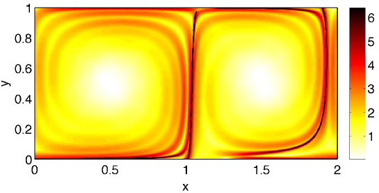
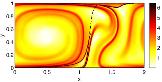
Figure 8: Finite-time Lyapunov exponent fields at $t=-0.9$ for (76) with $U=1$, $L=1$ and $T_{s}=-1$. The desired stable manifold (72) is shown by the black dashed curve, and the panels are respectively for the choices $\varepsilon=0.05,\,0.1,\,0.2$.

Thus, the claim is that (72) is the restricted stable manifold of the system

$$\left.\begin{array}[]{l}\dot{x}=-\pi U\sin\left(\frac{\pi x}{L}\right)\cos\left(\frac{\pi y}{L}\right)-\varepsilon Ue^{-Up(y,t)/L}\left[\sin\frac{U(t-p(y,t))}{L}+\pi^{2}\cos\frac{\pi y}{L}\cos\frac{U(t-p(y,t))}{L}\right]\\ \dot{y}=\pi U\cos\left(\frac{\pi x}{L}\right)\sin\left(\frac{\pi y}{L}\right)+\varepsilon U\sin\frac{\pi x}{L}\sin\frac{Ut}{L}\end{array}\right\}\,,$$ (76)

in which $p(y,t)$ is given in (71). The restrictions on the parameters are $U>0$, $L>0$, $\left|\varepsilon\right|\ll 1$, $-\infty<T_{s}<0$ and $-\infty<S$. The $p$ restriction for describing the manifold could alternatively be given as $y$-restriction $0<y<y_{m}(t)$, with $y_{m}(t)$ defined in (73). This is only a limitation of $y$ in describing the ${\mathcal{O}}(\varepsilon)-$close manifold; there is no restriction of $y$ in the flow (76).

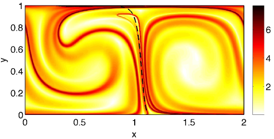
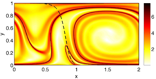
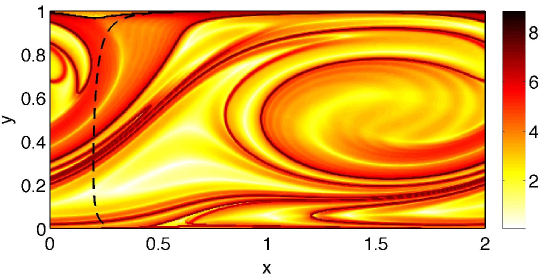
Figure 9: Finite-time Lyapunov exponent fields for (76) with $U=1$, $L=1$, $T_{s}=-1$ and $\varepsilon=0.1$. The desired stable manifold (72) is shown by the black dashed curve, and the panels are respectively for the choices $t=0.2,\,0.5,\,1.5$.

In order to test the validity of the analytical results, we compare them with numerically approximated manifolds for the system (76). For this we approximate the respective finite-time Lyapunov (FTLE) fields, choosing an integration interval $[t,t+1]$. Ridges in the FTLE field at $t$ indicate—under certain additional assumptions [6]—the location of stable manifolds. We refer to [28] for a brief explanation of the computational scheme used in this paper. Recent work by Haller [6] sets the heuristical FTLE approach on a sound mathematical basis.

In Fig. 8 we show the finite-time Lyapunov fields computed for the system (76) at $t=-0.9$, with the choice of parameters $U=1$, $L=1$ and $T_{s}=-1$. The black dashed curve indicates the desired stable manifold (72). This desired stable manifold matches up well with a ridge of the FTLE field, in particular, when $\varepsilon$ is sufficiently small. One clearly sees deviations for $y$ being close to $1$ in the two upper panels of Fig. 8. In the bottom panel, we have chosen a larger value of $\varepsilon$; here the alignment of the desired manifold and the numerically observed one breaks down already for small $y$. The lack of control of the manifold for larger $y$ is a reflection of the condition (73); the $\mathcal{O}(\varepsilon^{2})$-closeness of the desired manifold to the true manifold breaks down beyond this value.

In contrast, we investigate the worsening of the control strategy with time (at fixed $\varepsilon$) in Fig. 9. These and other experiments indicate that the control strategy works well in the range $T_{s}\leq t<T_{s}+1.3$ for this example. The reason for the worsening which occurs for larger values of t in this example can be explained by viewing the last panel ($t=1.5$) in Fig. 9. Here, the mappability of the required stable manifold is being compromised near the hyperbolic point along the $y=0$ line; the black dashed curve is becoming perpendicular to the line $x=1$ (which is the unperturbed stable manifold). Therefore, the domain $[S_{1}(t),S_{2}(t))$ associated with the legitimacy of the control strategy appears to be shrinking at such larger $t$ values.

7 Concluding remarks

We have in this article developed a theoretical framework based on which it is possible to move a stable/unstable manifold in a two-dimensional autonomous system, to a desired nonautonomous location which is subjected to certain mappability conditions to the original manifold. A rigorous error estimate for the procedure was developed. A numerical example is used to demonstrate the efficacy of the manifold control method. To our knowledge, this is the first study which furnishes a method for controlling stable and unstable manifolds nonautonomously in the sense of making them follow a user-specified time-variation.

In a forthcoming article, we will develop methods for simplifying the hypotheses required for the restricted stable and unstable manifolds, in order to address the computationally natural situation of attempting to achieve a desired stable/unstable manifold which is given in the form $f(x,y,t)=0$, as opposed to having to work through the parameter $p$. Preliminary results indicate that the control strategy can be implemented, for example, to achieve highly wiggly user-specified nonautonomous invariant manifolds. We expect to obtain insights into a more natural implementation of the mappability condition, so that unreasonable expectations from our control strategy (such as the dashed curve we tried to require in the final panel in Fig. 9) are avoided. Extensive numerical analyses will be performed in all these situations.

This article complements the authors’ work on controlling hyperbolic trajectories (that is, the “beginning of stable/unstable manifolds”). In ongoing research, recent two-dimensional control strategies [29] are being extended to arbitrary dimensions, and to arbitrarily high-order accuracy. Building on the present article, similarly extending control strategies to stable/unstable manifolds in high dimensions shall be our next focus.

Acknowledgements: This work was partially supported by a grant from the Simons Foundation (#236923 to SB), and by TU Dresden, in sponsoring a visit by SB to Dresden. A start-up grant from the University of Adelaide to SB is also gratefully acknowledged.

References

Haller and Beron-Vera [2012]
G. Haller, F. Beron-Vera,
Geodesic theory of transport barriers in
two-dimensional flows,
Phys. D 241
(2012) 1680–1702.
Blazevski and Haller [2013]
D. Blazevski, G. Haller,
Hyperbolic and elliptic transport barriers in
three-dimensional unsteady flows (2013).
arXiv: submit/0752347 (submitted).
Allshouse and Thiffeault [2012]
M. Allshouse, J.-L. Thiffeault,
Detecting coherent structures using braids,
Phys. D 241
(2012) 95–105.
Froyland and Padberg [2012]
G. Froyland, K. Padberg,
Finite-time entropy: a probabilistic method for
measuring nonlinear stretching,
Phys. D 241
(2012) 1612–1628.
Budis̆ić and Mezić [2012]
M. Budis̆ić, I. Mezić,
Geometry of ergodic quotient reveals coherent
structures in flows,
Phys. D 241
(2012) 1255–1269.
Haller [2011]
G. Haller,
A variational theory for Lagrangian Coherent
Structures,
Phys. D 240
(2011) 574–598.
Shadden et al. [2005]
S. Shadden, F. Lekien,
J. Marsden,
Definition and properties of Lagrangian coherent
structures from finite-time Lyapunov exponents in two-dimensional aperiodic
flows,
Phys. D 212
(2005) 271–304.
Dellnitz and Junge [1997]
M. Dellnitz, O. Junge,
Almost invariant sets in Chua’s circuit,
Int. J. Bif. Chaos 7
(1997) 2475–2485.
Froyland et al. [2010a]
G. Froyland, S. Lloyd,
N. Santitissadeekorn,
Coherent sets for nonautonomous dynamical systems,
Phys. D 239
(2010a) 1527–1541.
Froyland et al. [2010b]
G. Froyland, N. Santitissadeekorn,
A. Monahan,
Transport in time-dependent dynamical systems:
finite-time coherent sets,
Chaos 20
(2010b) 043116.
Mezić et al. [2010]
I. Mezić, S. Loire,
V. Fonoberov, P. Hogan,
A new mixing diagnostic and Gulf oil spill
movement,
Science 330
(2010) 486–489.
Balasuriya [2011]
S. Balasuriya,
A tangential displacement theory for locating
perturbed saddles and their manifolds,
SIAM J. Appl. Dyn. Sys. 10
(2011) 1100–1126.
Balasuriya [2013]
S. Balasuriya,
Nonautonomous flows as open dynamical sytems:
characterising escape rates and time-varying boundaries,
in: Ergodic Theory, Open Dynamics and
Structures, Springer, 2013.
In press.
Balasuriya [2012]
S. Balasuriya,
Explicit invariant manifolds and specialised
trajectories in a class of unsteady flows,
Phys. Fluids 24
(2012) 127101.
Farazmand and Haller [2012]
M. Farazmand, G. Haller,
Computing Lagrangian Coherent Structures from
variational LCS theory,
Chaos 22 (2012)
013128.
Peacock and Dabiri [2010]
T. Peacock, J. Dabiri,
Introduction to focus issue: Lagrangian Coherent
Structures,
Chaos 20 (2010)
017501.
Boffetta et al. [2001]
G. Boffetta, G. Lacorata,
G. Radaelli, A. Vulpiani,
Detecting barriers to transport: a review of
different techniques,
Phys. D 159
(2001) 58–70.
Krauskopf et al. [2005]
B. Krauskopf, H. Osinga,
E. Doedel, M. Henderson,
J. Guckenheimer, A. Vladimirsky,
M. Dellnitz, O. Junge,
A survey of method’s for computing (un)stable
manifold of vector fields,
Int. J. Bif. Chaos 15
(2005) 763–791.
Froyland [2013]
G. Froyland,
An analytic framework for identifying finite-time
coherent sets in time-dependent dynamical systems,
Phys. D 250
(2013) 1–19.
Radko [2011]
T. Radko,
On the generation of large-scale structures in a
homogeneous eddy field,
J. Fluid Mech. 668
(2011) 76–99.
Chandrasesekhar [1961]
S. Chandrasesekhar, Hydrodynamics and
hydrodynamic stability, Dover, New
York, 1961.
Balasuriya [2005a]
S. Balasuriya,
Approach for maximizing chaotic mixing in
microfluidic devices,
Phys. Fluids 17
(2005a) 118103.
Balasuriya [2005b]
S. Balasuriya,
Direct chaotic flux quantification in perturbed
planar flows: general time-periodicity,
SIAM J. Appl. Dyn. Sys. 4
(2005b) 282–311.
Balasuriya and Finn [2012]
S. Balasuriya, M. Finn,
Energy constrained transport maximization across a
fluid interface,
Phys. Rev. Lett. 108
(2012) 244503.
Coppel [1978]
W. A. Coppel, Dichotomies in Stability
Theory, number 629 in Lecture Notes in
Mathematics, Springer-Verlag,
Berlin, 1978.
Yi [1993]
Y. Yi,
A generalized integral manifold theorem,
J. Differential Equations 102
(1993) 153–187.
Yagasaki [2008]
K. Yagasaki,
Invariant manifolds and control of hyperbolic
trajectories on infinite- or finite-time intervals,
Dyn. Sys. 23
(2008) 309–331.
Padberg et al. [2007]
K. Padberg, T. Hauff,
F. Jenko, O. Junge,
Lagrangian structures and transport in turbulent
magnetized plasmas,
New J. Phys. 9
(2007) 400.
Balasuriya and Padberg-Gehle [2013]
S. Balasuriya, K. Padberg-Gehle,
Controlling the unsteady analogue of saddle
stagnation points,
SIAM J. Appl. Math. 73
(2013) 1038–1057.