Atom-molecule conversion system subject to phase noises

Abstract

The dynamics of atom-molecule conversion system subject to dephasing noises is studied in this paper. With the dephasing master equation and the mean-field theory, we drive a Bloch equation for the system, this equation is compared with the Bloch equation derived by the Bogoliubov-Born-Green-Kirkwood-Yvon (BBGKY) hierarchy truncation approach. Fixed points of the system are calculated by solving both the Bloch equations and the master equation, comparison between these two calculations suggests that while in a short time the mean-field theory is a good approximation for the atom-molecule conversion system, a high order hierarchy truncation approach is necessary for the system in a long time scale. Although the MFT can not predict correctly the fixed points, its prediction on the stability of the fixed points are consistent with the BBGKY theory for a wide range of parameters.

I Introduction

In the realm of ultracold atom-molecule physics, association of ultracold atoms into diatomic molecules is an attractive subject. It inspires many interests due to its applications ranging from the production of molecule Bose-Einstein condensates (BECs) to the study of chemical reaction and permanent electric dipole moments Greiner2003 ; Heinzen2000 ; Zwierlein2003 ; Regal2004 ; Junker2008 ; Jing2009 ; Qian2010 ; Inouye1998 . Coherent oscillations between an atomic BEC and a molecular BEC have been theoretically predictedTimmermans1999prl2691 ; Javanainen1999 by the use of Gross-Pitaevskii (GP) equations Vardi2001pra1 ; Santos2006 ; Li2009 ; Liu2010 ; Santos2010 ; Fu2010 , the results suggest that the mean-field theory is a good formalism to describe the conversion of atoms to molecules in the absence of noise Timmermans1999prl199 ; Kohler2006 .

The noise may come from the inelastic collisions between the atoms in the condensates and that in the non-condensate atoms, local fluctuations and non-local fluctuations. The noise may also come from the random variation of the atom-molecule detuning or magnetic field fluctuations in the Feshbach-resonance setupKhripkov2011 ; Timmermans1999prl199 ; Duine2004 ; Brouard2005 . The presence of noise can dephase the Bose-Einstein condensates and strongly limit the validity of the Gross-Pitaevskii(GP) equations. There have been several theoretical studied going beyond the GP equations, for example, based on the time-dependent field theory, the dynamics of the atom-molecule conversion system was studied in Javanainen2002 ; Naidon2008 , where the noise comes from nonlocal fluctuations due to the time-dependent pair correlations, and within the two-model approximation, the authors in Ref. Khripkov2011 ; Cui2012 explored the master equation to investigate the atom-molecule conversion system.

Earlier study on a bimodal decoherence-free condensate show that the mean-field theory(MFT) may fail near the dynamical instabilityAnglin2001 ; Vardi2001prl568 , this inspires us to explore whether the MFT is valid for the atom-molecule conversion system with noise (dissipation and dephasing). The effect of dissipation on the dynamics of the atom-molecule conversion system was studied in Cui2012 . In this paper we will focus on the effect of dephasing within the two-mode approximation. We show that the dynamics of the dephasing atom-molecule conversion system is well treated by the MFT in a short time scale, but it fails to give a correct prediction about the system at a long time scale. This suggests us to use the high order of BBGKY hierarchy truncationAnglin2001 ; Vardi2001prl568 to explore the atom-molecule conversion system subject to dephasing noises.

The remainder of the paper is organized as follows. In Sec. II, we introduce the dephasing master equation and derive a Bloch equation for the system, the solution of the Bloch equation without dephasing is presented and discussed. In Sec. III, we calculate the fixed points of the system with the MFT and compare these fixed points with that by analytically solving the master equation. The Bloch equation derived from the BBGKY hierarchy equation is presented in Sec. IV. In Sec. V, we discuss the stability and the feature of the fixed points from both the MFT and the BBGKY hierarchy truncation. Discussion and conclusions are given in Sec. VI.

II Model

We consider the simplest model for the atom-molecule conversion system. By the two-mode approximation, the model Hamiltonian can be written asKhripkov2011 ; Vardi2001pra1 ; Kostrun2000

$$\hat{H}=\frac{\varepsilon}{2}\hat{a}^{\dagger}\hat{a}+\frac{g}{2}(\hat{a}^{\dagger}\hat{a}^{\dagger}\hat{b}+\hat{b}^{\dagger}\hat{a}\hat{a}),$$ (1)

where $\hat{a}$ and $\hat{b}$ represent annihilation operators for atom and molecule, respectively, $g$ denotes the strength of the atom-molecule conversion, and $\varepsilon$ is the atomic binding energy.

The master equation taking only the dephasing noise into account may be written into the following formKhripkov2011 ; Anglin1997

$$\dot{\rho}=-i[\hat{H},\rho]-\Gamma[\hat{\ell},[\hat{\ell},\rho]],$$ (2)

where $\hat{\rho}$ is the density matrix of system, $\Gamma$ is the dephasing rate, the Lindblad operator $\hat{\ell}$ is the population difference,

$$\hat{\ell}=2\hat{b}^{\dagger}\hat{b}-\hat{a}^{\dagger}\hat{a}.$$ (3)

The total atom number operator $\hat{N}=2\hat{b}^{\dagger}\hat{b}+\hat{a}^{\dagger}\hat{a}$ is conserved since $\frac{\partial\left\langle\hat{N}\right\rangle}{\partial t}=0,$ so the total atom number $N$ is a constant that does not change with time in the dynamics. Define,

$${{\hat{L}}_{x}} = \sqrt{2}\frac{{{{\hat{a}}^{\dagger}}{{\hat{a}}^{\dagger}}\hat{b}+{{\hat{b}}^{\dagger}}\hat{a}\hat{a}}}{{{N^{3/2}}}},$$

$${{\hat{L}}_{y}} = \sqrt{2}i\frac{{{{\hat{a}}^{\dagger}}{{\hat{a}}^{\dagger}}\hat{b}-{{\hat{b}}^{\dagger}}\hat{a}\hat{a}}}{{{N^{3/2}}}},$$

$${{\hat{L}}_{z}} = \frac{{2{{\hat{b}}^{\dagger}}\hat{b}-{{\hat{a}}^{\dagger}}\hat{a}}}{N},$$ (4)

where $\hat{L}_{z}$ denotes the number difference between the atoms and the molecules in the system, $\hat{L}_{x}$ and $\hat{L}_{y}$ can be used to characterize the coherence of atom-molecule conversion. It is easy to prove that,

$$\left[\hat{L}_{z},\hat{L}_{x}\right] = \frac{4i}{N}\hat{L}_{y},$$

$$\left[\hat{L}_{z},\hat{L}_{y}\right] = -\frac{4i}{N}\hat{L}_{x},$$

$$\left[\hat{L}_{x},\hat{L}_{y}\right] = \frac{i}{N}(1-\hat{L}_{z})(1+3\hat{L}_{z})+\frac{4i}{N^{2}}.$$ (5)

Notice that $\hat{L}_{x},\hat{L}_{y},\hat{L}_{z}$ are not the SU(2) generators, because their commutation relations contain quadratic terms of $\hat{L}_{z}.$ Nevertheless, in the small atom-molecule number difference and large $N$ limit ($N\rightarrow\infty$), $\hat{L}_{x}$, $\hat{L}_{y}$ and $\hat{L}_{z}$ really form a sphere since they satisfy,

$${({{\hat{L}}_{x}})^{2}}+{({{\hat{L}}_{y}})^{2}} = \frac{1}{2}(1+{{\hat{L}}_{z}}){(1-\hat{L}{\ {}_{z}})^{2}}$$ (6)

$$+ \frac{2}{N}(1-{{\hat{L}}_{z}})+\frac{4}{{{N^{2}}}}{{\hat{L}}_{z}}.$$

We will call this sphere the generalized Bloch sphere even when the system is far from the limits. With these definitions, the Hamiltonian becomes $\hat{H}=-\frac{\varepsilon}{4}N\hat{L}_{z}+\frac{g}{2\sqrt{2}}N^{3/2}\hat{L}_{x},$ and the master equation can be rewritten as

$$\dot{\rho}=-i[\hat{H},\rho]-\Gamma{N^{2}}[{\hat{L}_{z}},[{\hat{L}_{z}},\rho]].$$ (7)

From this master equation, the expectation values defined by $F_{i}=$ $\langle{\hat{L}_{i}}\rangle=Tr(\rho{\hat{L}_{i}}),i=x,y,z$ follow,

$$\frac{{\partial{F_{x}}}}{{\partial t}} = \varepsilon{F_{y}}-16\Gamma{F_{x}},$$

$$\frac{{\partial{F_{y}}}}{{\partial t}} = -\varepsilon{F_{x}}-\Delta{F_{z}}+\frac{3}{2}\Delta\langle\hat{L}_{z}^{2}\rangle-16\Gamma{F_{y}}-R,$$

$$\frac{{\partial{F_{z}}}}{{\partial t}} = 2\Delta{F_{y}},$$ (8)

where $\Delta=g\sqrt{\frac{N}{2}},$ and $R=\frac{1}{2}\Delta+\frac{2\Delta}{N}.$ The lowest-order truncation of Eq. (8) is acquired by approximating the second-order expectation values $\langle\hat{L}_{i}\hat{L}_{j}\rangle$ as products of the first-order expectations $\langle\hat{L}_{i}\rangle$ and $\langle\hat{L}_{j}\rangle$ Anglin2001 , namely,

$$\langle\hat{L}_{i}\hat{L}_{j}\rangle\approx\langle\hat{L}_{i}\rangle\langle\hat{L}_{j}\rangle,$$ (9)

with this approximation, Eq. (8) reduces to,

$$\frac{{\partial{F_{x}}}}{{\partial t}} = \varepsilon{F_{y}}-16\Gamma{F_{x}},$$

$$\frac{{\partial{F_{y}}}}{{\partial t}} = -\varepsilon{F_{x}}-\Delta{F_{z}}+\frac{3}{2}\Delta F_{z}^{2}-16\Gamma{F_{y}}-R,$$

$$\frac{{\partial{F_{z}}}}{{\partial t}} = 2\Delta{F_{y}}.$$ (10)

Next we discuss the situation with zero dephasing rate, $\Gamma=0$, Eq. (10) follows,

$$\frac{{\partial{F_{x}}}}{{\partial t}} = \varepsilon{F_{y}},$$

$$\frac{{\partial{F_{y}}}}{{\partial t}} = -\varepsilon{F_{x}}-\Delta{F_{z}}+\frac{3}{2}\Delta F_{z}^{2}-R,$$

$$\frac{{\partial{F_{z}}}}{{\partial t}} = 2\Delta{F_{y}}.$$ (11)

Define $a=\varepsilon^{2}+g^{2}N,$ $b=-\frac{3}{2}g^{2}N,$ and $c=\frac{g^{2}N}{2}+2g^{2}-\varepsilon^{2}F_{z0}$ with $F_{z0}$ the initial value of $F_{z}$, the solution of Eq. (11) can be obtained by solving,

$$\frac{\partial^{2}F_{z}}{\partial^{2}t}+aF_{z}+bF_{z}^{2}+c=0.$$ (12)

We notice that $b$ must not be zero here, otherwise $g=0$, which would result in $\Delta=0$ leading to ${\dot{F}_{z}(t)}=0,$ then $F(t)_{z}\equiv F_{z0}$, i.e., the state of system remains unchanged. The solution of Eq. (12) is,

$$F_{z}=u_{2}-(u_{2}-u_{3})cn^{2}(k(t-t_{0}),m)-\frac{a-A}{2b},$$ (13)

where $cn(k(t-t_{0}),m)$ is the Jacobi elliptic cosine function. $u_{1}>u_{2}>u_{3}$ and $u_{1}=n\cos\theta-\frac{A}{{2B}},$ $u_{2}=n\cos(\theta+\frac{4\pi}{3})-\frac{A}{{2B}},$ $u_{3}=n\cos(\theta+\frac{2\pi}{3})-\frac{A}{{2B}},$ $n=\frac{{A}}{{B}},$ $\cos(3\theta)=-\frac{1}{2}\left({d{{\left({\frac{{2B}}{A}}\right)}^{3}}+2}\right),$ $A=\sqrt{a^{2}-4bc},$ $B=b,$ $d=-u_{0}^{3}-\frac{{3A}}{{2B}}u_{0}^{2}$, and ${u_{0}}={F_{z0}}+\frac{{a-A}}{{2b}}$.

$F_{z}(t)$ is a periodic function of time with period $T=\frac{2K(m)}{k}$, $k=\sqrt{\frac{{-B({u_{1}}-{u_{3}})}}{6}}$, and $K(m)=\int_{0}^{\frac{\pi}{2}}{\frac{1}{{\sqrt{1-{m^{2}}{{\sin}^{2}}(\varphi)}}}}d\varphi$ being the first kind Legendre’s complete elliptic integral. ${t_{0}}$ denotes the time when $F_{z}$ takes $F_{z0}$ that can be determined by solving Eq. (13). Eq.  (11) describes a rotation of the Bloch vector $\mathbf{F}$, obviously the norm $\left|\mathbf{F}\right|$ is conserved in the MFT when the dephasing rate is zero.

In Fig. 1, we plot the ratio of $N_{a}$ to $N$ as a function of time. Two results are presented, one comes from Eq. (13), and another is obtained by solving the master equation with $\Gamma=0$ numerically. We find that at a short time scale, the two results are in good agreement, however, at a long time scale, the two results are evidently different. This suggests that the MFT is a good approximation to describe the dynamics of the atom-molecule conversion system at a short time scale. Besides, the binding energy of the atom can turn the system from self-trapping regime (Fig 1 (a)) to tunneling regime (Fig 1 (b)). This can be understood as a conversion blockage due to the energy difference between the atoms and molecules. Note that the binding energy of the molecules is zero.

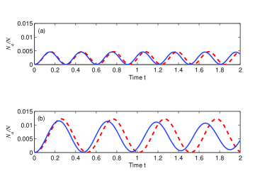
Figure 1: (Color online) The number of atoms in the atomic mode as a function of time. The red-dashed line represents Eq. (13), which is an analytical solution of the Bloch equation with $\Gamma=0$ based on the mean-field theory. In contrast, the numerical simulation of the Liouville equation (2) with $\Gamma=0$ is shown by the blue-solid line with ${F_{z0}}=1,{F_{x0}}={F_{y0}}=0$ at time $t=0$. Here and hereafter, $\varepsilon$ and $\Gamma$ are rescaled in units of $g$, and $t$ is then in units of $1/g$. Hence all parameters are of dimensionless. $N=100$. (a) and (b) are for different $\varepsilon$. (a) $\varepsilon=25,$ and (b) $\varepsilon=19.$

III Steady state and fixed points

The fixed point of the system is defined by

$${{\dot{F}}_{x}}={{\dot{F}}_{y}}={{\dot{F}}_{z}}=0.$$ (14)

By this definition, we can obtain the fixed points in the MFT,

$${F_{xf}}={F_{yf}}=0,{F_{zf}}=\frac{1}{3}\left({1-\sqrt{1+3\left({1+{4\mathord{\left/{\vphantom{4N}}\right.\kern-1.2pt}N}}\right)}}\right).$$ (15)

On the other hand, we can obtain the steady state by analytically solving the master equation Eq. (2). Once we have the steady state of the system, the fixed points can be calculated by the definition of $F_{j}.$ The steady state ${\rho_{s}}$ satisfies the following equation,

$${{\dot{\rho}}_{s}}=-i[\hat{H},{\rho_{s}}]{\rm{+}}\Gamma\left({2\hat{\ell}{\rho_{s}}\hat{\ell}-\hat{\ell}\hat{\ell}{\rho_{s}}-{\rho_{s}}\hat{\ell}\hat{\ell}}\right)=0.$$ (16)

It is easy to prove that the off-diagonal elements of density matrix vanish in the steady state due to the dephasing. The proof is as follows. Define Fock states $\left|n\right\rangle\equiv\left|{N-2n,n}\right\rangle$ denoting $(N-2n)$ atoms and $n$ molecules (${{n=0,1,2,}}\cdots{{N/2}}$), we have the following equation for the off-diagonal elements of the density matrix,

$$\frac{{\partial{\rho_{mn}}}}{{\partial t}}+i\left({{a_{m}}-{a_{n}}}\right){\rho_{mn}}$$

$$+16\Gamma{\left({m-n}\right)^{2}}{\rho_{mn}}+\xi\left(t\right)=0,$$ (17)

where $\xi\left(t\right)=i({b_{m}}{\rho_{m-1n}}+{c_{m}}{\rho_{m+1n}}-{b_{n}}{\rho_{mn-1}}-{c_{n}}{\rho_{mn+1}})$, ${a_{n}}=\frac{\varepsilon}{2}(N-2n)$, ${b_{n}}=\frac{g}{2}(\sqrt{\left({N-2n+1}\right)\left({N-2n+2}\right)\left(n\right)})$, and ${c_{n}}=\frac{g}{2}(\sqrt{\left({N-2n}\right)\left({N-2n-1}\right)\left({n+1}\right)})$. The formal solution of Eq. (17) is

$${\rho_{mn}}={e^{-\left({i\left({{a_{m}}-{a_{n}}}\right)+16\Gamma{{\left({m-n}\right)}^{2}}}\right)t}}[\Xi-\int\xi(t){e^{\left({i\left({{a_{m}}-{a_{n}}}\right)+16\Gamma{{\left({m-n}\right)}^{2}}}\right)t}}dt],$$ (18)

where $\Xi$ is a constant determined by the initial condition of ${{\rho_{mn}}}$. We find that when $t\to\infty$, ${\rho_{mn}}\to 0\left({m\neq n}\right)$. This gives the steady state,

$${\rho_{s}}=\sum\limits_{n=0}^{N/2}{{\rho_{n}}}\left|n\right\rangle\left\langle n\right|.$$ (19)

For the steady state, it is required that $[\hat{H},{\rho_{s}}]=0$, from which we obtain ${\rho_{j}}={\rho_{j-1}}$. This together with $Tr{\rho_{s}}=1$, we obtain ${\rho_{0}}={\rho_{1}}={\rho_{2}}=\cdots={\rho_{N/2}}=\frac{1}{{N/2+1}}$. Collecting all together, we have,

$${\rho_{s}}=\sum\limits_{n=0}^{N/2}{\left({\frac{1}{{N/2+1}}}\right)\left|n\right\rangle\left\langle n\right|,}$$ (20)

The fixed points ${F_{is}},\ (i=x,y,z)$ of the system can be given by the steady state Eq. (20) as ${{F_{zs}}=Tr({\rho_{s}}{{\hat{L}}_{z}})=\sum\limits_{n=0}^{N/2}{{{\hat{L}}_{z}}}(\frac{1}{{N/2+1}})\left|n\right\rangle\langle n|=0}.$ In the same way, ${F_{xs}}={F_{ys}}=0$. Namely, the fixed point given by solving the master equation is,

$${F_{xs}}={F_{ys}}={F_{zs}}=0.$$ (21)

It is easy to find that the fixed points given by the MFT and the master equation are different. This indicates that the MFT is not a good approach to describe the atom-molecule conversion system at a long time scale. This stimulates us to use the BBGKY hierarchy truncationAnglin2001 ; Vardi2001prl568 to study the system.

IV The BBGKY hierarchy of equations of motion

As aforementioned, the differential equation for the Bloch vector up to the first order is not a good treatment at a long time scale. Thus high order expectation values is required. In this section, we will obtain an improved theory to the MFT using the next order of the Bogoliubov-Born-Green-Kirkwood-Yvon (BBGKY) hierarchy of equation of motion.

Writing $\langle\hat{L}_{z}^{2}\rangle$ in Eq. (8) in terms of the following expectation value,

$$K_{ij}=\langle\hat{L}_{i}\hat{L}_{j}+\hat{L}_{j}\hat{L}_{i}\rangle-2\langle\hat{L}_{i}\rangle\langle\hat{L}_{j}\rangle,i,j=x,y,z,$$ (22)

and truncating the BBGKY hierarchy of equations of motion for the first- and second-order operators $\hat{L}_{i},\hat{L}_{i}\hat{L}_{j}$ Anglin2001 ; Vardi2001prl568 ,

$$\langle{{\hat{L}}_{i}}{{\hat{L}}_{j}}{{\hat{L}}_{k}}\rangle \approx \langle{{\hat{L}}_{i}}{{\hat{L}}_{j}}\rangle\langle{{\hat{L}}_{k}}\rangle+\langle{{\hat{L}}_{i}}\rangle\langle{{\hat{L}}_{j}}{{\hat{L}}_{k}}\rangle$$ (23)

$$+ \langle{{\hat{L}}_{i}}{{\hat{L}}_{k}}\rangle\langle{{\hat{L}}_{j}}\rangle-2\langle{{\hat{L}}_{i}}\rangle\langle{{\hat{L}}_{j}}\rangle\langle{{\hat{L}}_{k}}\rangle,$$

we get the following set of equations for the first- and second-order moments,

$$\frac{{\partial{F_{x}}}}{{\partial t}} = \varepsilon{F_{y}}-16\Gamma{F_{x}},$$

$$\frac{{\partial{F_{y}}}}{{\partial t}} = -\varepsilon{F_{x}}-\Delta{F_{z}}+\frac{3}{2}\Delta\left({\frac{1}{2}{K_{zz}}+F_{z}^{2}}\right)-16\Gamma{F_{y}}-R$$

$$\frac{{\partial{F_{z}}}}{{\partial t}} = 2\Delta{F_{y}},$$

$$\frac{{\partial{K_{xx}}}}{{\partial t}} = 2\varepsilon{K_{xy}}-32\Gamma{K_{xx}}+32\Gamma{K_{yy}}+64\Gamma F_{y}^{2},$$

$$\frac{{\partial{K_{yy}}}}{{\partial t}} = -2\varepsilon{K_{xy}}-2\Delta{K_{yz}}+6\Delta{F_{z}}{K_{yz}}-32\Gamma{K_{yy}}$$

$$+ 32\Gamma{K_{xx}}+64\Gamma F_{x}^{2},$$

$$\frac{{\partial{K_{zz}}}}{{\partial t}} = 4\Delta{K_{yz}},$$

$$\frac{{\partial{K_{xy}}}}{{\partial t}} = -\varepsilon{K_{xx}}-\Delta{K_{xz}}+3\Delta{F_{z}}{K_{xz}}+\varepsilon{K_{yy}}-64\Gamma{K_{xy}}$$

$$- 64\Gamma{F_{x}}{F_{y}},$$

$$\frac{{\partial{K_{yz}}}}{{\partial t}} = 2\Delta{K_{yy}}-\varepsilon{K_{xz}}-\Delta{K_{zz}}+3\Delta{F_{z}}{K_{zz}}-16\Gamma{K_{yz}}$$

$$\frac{{\partial{K_{xz}}}}{{\partial t}} = 2\Delta{K_{xy}}+\varepsilon{K_{yz}}-16\Gamma{K_{xz}}.$$ (24)

Eq. (24) was called Bogoliubov backreaction equationsAnglin2001 ; Vardi2001prl568 (BBR), because the fluctuations $K_{ij}$ are driven by the mean-field Bloch vector F, which is physically described by the Bogoliubov theory. In turn, the Bloch vector is affected by the fluctuations $K_{\text{ij}}$. This backreaction makes the trajectory of the system not confined to the surface of the generalized Bloch sphere, which is a reminiscence of the effect of dephasing.

We plot the time evolution of the atom number ${N_{a}}$ and the fluctuation ${K_{{{zz}}}}$ given by BBR and MFT in Fig. 2. The results from numerically solving the master equation Eq. (2) is also presented. To plot the figure, the following initial condition

$$\begin{array}[]{l}{F_{z}}=-1,\\ {K_{xx}}={K_{yy}}=4\left({N-1}\right)/{N^{2}},\\ {F_{x}}={F_{y}}={K_{zz}}={K_{xy}}={K_{xz}}={K_{yz}}=0\end{array}$$ (28)

is taken, the corresponding quantum state is the molecular vacuum state $\left|N,0\right\rangle$.

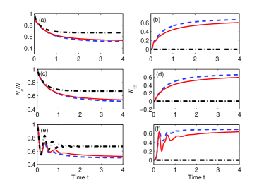
Figure 2: (Color online) $N_{a}/N$ and $K_{zz}$ versus time. The results are obtained by the mean-field theory (black-dash-dotted line), Bogoliubov backreaction equations (red-solid line), and the numerical solution of the master equation (blue-dashed line). The initial condition of the system are the same as in Eq. (28). Parameters chosen are $g=1,N=100,\varepsilon=30,\Gamma=1$ for (a) and (b), $\varepsilon=40,\Gamma=1.8$ for (c) and (d), and $\varepsilon=10,\Gamma=0.2$ for (e) and (f).

We find that the results given by the BBR equations are in good agreement with that by numerically solving the master equation. The results by the MFT are different from those at a long time scale. This difference comes from the fluctuations $K_{ij}$, which are ignored in the MFT. Noticing the fixed points given by the BBR equations are the same as that by the numerical method but different from those by MFT, we emphasize that the stability of the fixed points by MFT and BBR equations are the same for a wide range of parameters in the space spanned by $F_{x}$, $F_{y}$ and $F_{z}$, this is due to the linear coupling between the Bloch vector F and the fluctuations $K_{ij}$ in F, see the first three equations in Eq.(24).

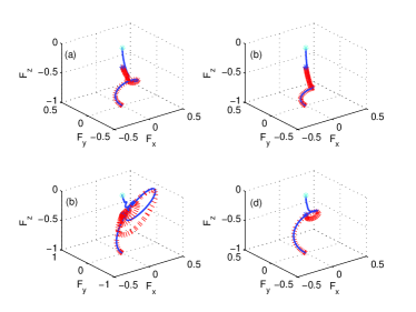
Figure 3: (Color online) $F_{z}$ as a function of time by the mean-field theory (red-dotted line) and Bogoliubov backreaction equation (blue-solid line). The black-star denotes the fixed point by the MFT in Eq. (10) and the green-star denotes the fixed point by BBR in Eq. (24). The parameters of (a), (b) and (c) are the same as in Fig. 2. In figure (d), $g=1,\varepsilon=15,\Gamma=0.8,N=100$.

V Stability of the fixed points with $\varepsilon=0$

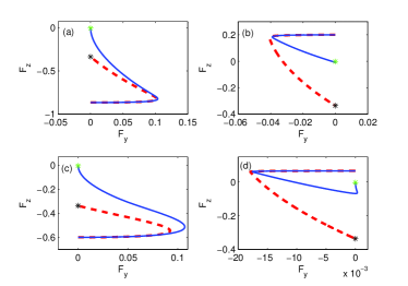
Figure 4: (Color online) This plot shows the fixed points and how the system approaches the fixed points. The black and green stars denote the location of the stable junction fixed point by the MFT and by the BBR (see, Eq. (40)), respectively. The red-dashed line (MFT) and the blue-solid line(BBR) show how the system approaches the fixed points. The initial state of the system is $\left|{{\psi_{0}}}\right\rangle=\left|n\right\rangle$. Parameters chosen are $g=1,\Gamma=10,N=300$, $\left|{{\psi_{0}}}\right\rangle=\left|{10}\right\rangle$ for (a), $\Gamma=12,$ $\left|{{\psi_{0}}}\right\rangle=\left|{90}\right\rangle$ for (b), $\Gamma=4$, $\left|{{\psi_{0}}}\right\rangle=\left|{30}\right\rangle$ for (c) and $\Gamma=24$, $\left|{{\psi_{0}}}\right\rangle=\left|{80}\right\rangle$ for (d).

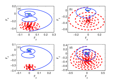
Figure 5: (Color online) Black star and green star denote the location of the stable focus fixed points predicted by MFT and BBR, respectively. The red-dashed (MFT) and the blue-solid (BBR) show the trajectories for the system from initial state to fixed points. Parameters chosen are $g=1,\Gamma=0.12,N=300$, $\left|{{\psi_{0}}}\right\rangle=\left|{40}\right\rangle$ for (a), $\Gamma=0.2$, $\left|{{\psi_{0}}}\right\rangle=\left|{82}\right\rangle$ for (b), $\Gamma=0.16$, $\left|{{\psi_{0}}}\right\rangle=\left|{45}\right\rangle$ for (c), and $\Gamma=0.1$, $\left|{{\psi_{0}}}\right\rangle=\left|{100}\right\rangle$ for (d).

In this section, we will discuss stability of the fixed points from both the MFT and the BBGKY hierarchy. For the reason of simplicity, let us consider the situation of zero atomic binding energy, $\varepsilon=0$. In this case, Eq. (10) reduces to,

$$\begin{array}[]{l}\frac{{\partial{F_{y}}}}{{\partial t}}=-\Delta{F_{z}}+\frac{3}{2}\Delta F_{z}^{2}-16\Gamma{F_{y}}-R,\\ \frac{{\partial{F_{z}}}}{{\partial t}}=2\Delta{F_{y}}.\end{array}$$ (31)

By the Jacobian matrix defined by

$$J={\left({\begin{array}[]{*{20}{c}}{\frac{{\partial P}}{{\partial{F_{y}}}}}&{\frac{{\partial P}}{{\partial{F_{z}}}}}\\ {\frac{{\partial Q}}{{\partial{F_{y}}}}}&{\frac{{\partial Q}}{{\partial{F_{z}}}}}\end{array}}\right)_{\left({{F_{xf}},{F_{yf}},{F_{zf}}}\right)}},$$ (34)

we can study the stability of the fixed points in the MFT. Here $P=-\Delta F_{z}+\frac{3}{2}\Delta F_{z}^{2}-16\Gamma F_{y}-R$, $Q=2\Delta F_{y}$. The eigenvalues of the Jacobi matrix $J$ would determine the stability of the fixed points, which can be given by simple calculations, $\lambda_{\pm}=\frac{1}{2}(-16\Gamma\pm\sqrt{256{\Gamma^{2}}-4N{g^{2}}(1-3{F_{zf}})})=\frac{1}{2}(-16\Gamma\pm\sqrt{256{\Gamma^{2}}-{\rm{4}}N{g^{2}}\sqrt{1{\rm{+}}3(1{\rm{+}}4/N)}})$. If it is satisfied that

$$64{\Gamma^{2}}\geq N{g^{2}}\sqrt{1{\rm{+}}3\left({1{\rm{+}}4/N}\right)},$$ (35)

Jacobi matrix $J$ has two negative roots, the fixed point (15) is a stable junction fixed point. When

$$64{\Gamma^{2}}\leq N{g^{2}}\sqrt{1{\rm{+}}3\left({1{\rm{+}}4/N}\right)},$$ (36)

Jacobi matrix $J$ has two conjugate complex roots, in this case the fixed point (15) is a stable focus fixed point.

Now we turn our discussion to the fixed points given by the BBGKY hierarchy of equation of motion. To compare the stability of fixed points by the BBGKY with the prediction by the MFT, we restrict the discussion in the space spanned by $F_{x}$, $F_{y}$ and $F_{z}$. This means that the fluctuations which drive the system away from the fixed points (steady state) occur only in $F_{x}$, $F_{y}$ and $F_{z}$. We start with the fixed points in the 9-dimensional space. By the same definition as in the MFT, we obtain the fixed point in the BBGKY Eq. (24) ($\varepsilon=0$)

$$\begin{array}[]{l}{F_{xB}}={F_{yB}}={F_{zB}}={K_{xzB}}={K_{xyB}}={K_{yzB}}=0,\\ {K_{zzB}}=\frac{2}{3}+\frac{8}{{3N}},\\ {K_{xxB}}={K_{yyB}}=\frac{1}{2}{K_{zzB}}.\end{array}$$ (40)

As mentioned, we discuss the case where fluctuations are only in $F_{x}$, $F_{y}$ and $F_{z}$. For $\varepsilon=0$, $F_{x}$ decouples with $F_{y}$ and $F_{z}$, then the discussion reduce to discuss fluctuations only in $F_{y}$ and $F_{z}$,

$$\begin{array}[]{l}{F_{y}}\to{F_{yB}}+\delta{f_{y}},\\ {F_{z}}\to{F_{zB}}+\delta{f_{z}},\end{array}$$ (43)

Substituting Eq. (43) into Eq. (24), we have,

$$\frac{{\partial\delta{f_{y}}}}{{\partial t}} = -\varepsilon\delta{f_{x}}-\Delta\delta{f_{z}}+\frac{3}{2}\Delta\left({\frac{1}{2}{K_{zzB}}+2{F_{zB}}\delta{f_{z}}}\right)$$

$$- 16\Gamma\delta{f_{y}}-R,$$

$$\frac{{\partial\delta{f_{z}}}}{{\partial t}} = 2\Delta\delta{f_{y}}.$$ (44)

By the same discussion as in Eq. (34), the Jacobian matrix in this case is,

$$J^{\prime}={\left({\begin{array}[]{*{20}{c}}{\frac{{\partial P^{\prime}}}{{\partial\delta{f_{y}}}}}&{\frac{{\partial P^{\prime}}}{{\partial\delta{f_{z}}}}}\\ {\frac{{\partial Q^{\prime}}}{{\partial\delta{f_{y}}}}}&{\frac{{\partial Q^{\prime}}}{{\partial\delta{f_{z}}}}}\end{array}}\right)_{\left({{F_{xB}},{F_{yB}},{F_{zB}}}\right)}},$$ (47)

where

$$P^{\prime}=-\varepsilon\delta{f_{x}}-\Delta\delta\ {f_{z}}+\frac{3}{2}\Delta\left({\frac{1}{2}{K_{zzB}}+2\ {F_{zB}}\delta{f_{z}}}\right)$$

$$-16\Gamma\delta{f_{y}}-R,$$

and $Q^{\prime}=2\Delta\delta{f_{y}},$ the eigenvalues of the Jacobi matrix $J^{\prime}$ are $\lambda^{\prime}_{\pm}=\frac{1}{2}(-16\Gamma\pm\sqrt{256{\Gamma^{2}}-4N{g^{2}}(1-3{F_{zB}}})=\frac{1}{2}(-16\Gamma\pm\sqrt{256{\Gamma^{2}}-4N{g^{2}}}).$ If

$$64{\Gamma^{2}}\geq N{g^{2}},$$ (48)

all $\lambda^{\prime}_{\pm}$ are negative, the fixed point (40) is a stable junction fixed point. Otherwise if

$$64{\Gamma^{2}}\leq N{g^{2}},$$ (49)

$\lambda^{\prime}_{\pm}$ are complex and their real parts are negative, the fixed point (40) is then a stable focus fixed point.

When the parameters satisfy simultaneously Eq. (35) and Eq. (48), the stability of the fixed points are the same in the MFT and the BBGKY, i.e., the fixed points are stable junction point, see Fig. 4. In this situation, the system approaches the fixed points straightforwardly. When the parameters satisfy both Eq. (36) and Eq. (49), the stability of the fixed points in the MFT and the BBGKY are also the same. The fixed points in this case are stable focus fixed point. The system go to the fixed points wavily.

When the parameters fall in the range of

$$N{g^{2}}<64{\Gamma^{2}}<N{g^{2}}\sqrt{1{\rm{+}}3\left({1{\rm{+}}4/N}\right)},$$ (50)

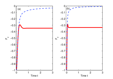
Figure 6: (Color online) Red-thick line shows how the system goes to the stable focus fixed points by MFT, while blue-dashed line shows how the system goes to the stable junction fixed point by the BBGKY in Eq. (24). Parameters chosen satisfying the Eq. (50) are $g=1,N=80$, $\Gamma=1.1192$, $\left|{{\psi_{0}}}\right\rangle=\left|{0}\right\rangle$ for (a), and $\Gamma=3.9568,N=1000$, $\left|{{\psi_{0}}}\right\rangle=\left|{0}\right\rangle$ for (b).

the system in the BBGKY theory Eq. (24) would go to a stable junction fixed point , but by the MFT, the system would approach to a stable focus fixed point. We plot the time evolution of ${F_{z}}$ in Fig. 6. From the figure, we can see that the population difference ${F_{z}}$ in BBGKY theory increases monotonously as $t$ increases (the blue-dashed line), but it increases first then decreases and finally reaches the stable state in the MFT. In addition, comparing Fig. (6) (a) and (b), we can learn that in (a) $F_{z}$ changes slowly, while in (b) it is faster, this is due to the difference of the dephasing rate $\Gamma$.

Before concluding the paper, we present a discussion on the time-dependent many-body theory Javanainen2002 ; Naidon2008 and the master equation approach in the two-mode approximation. We start with the many-body description for the photoassociation in a uniform Bose-Einstein condensate Naidon2008 . In the two-body case, the system model reduces to a set of coupled modes, two of them are atoms in condensate and molecules. The other modes represent the noncondensate atom pairs. This treatment is very similar to the master equation description, when the noncondensate atom pairs are treated as an environment. Then the elimination of the modes of noncondensate atom pairs in the two-body theory would lead to equations of motion (almost) equivalent to that in the master equation description.

To be specific, we take the photoassociation of a Bose-Einstein condensate Javanainen2002 as an example. The equation of motion of the system reads,

$$\dot{\alpha} = i\frac{\Omega}{\sqrt{2}}\,\alpha^{*}\beta,$$

$$\dot{\beta} = i\delta\beta+i\frac{\Omega^{*}}{\sqrt{2}}\,\alpha^{2}+i\int d\epsilon\,\xi(\epsilon)\,c_{\epsilon},$$

$$\dot{c}_{\epsilon} = -i\epsilon\,c_{\epsilon}+i\xi^{*}(\epsilon)\beta\,$$ (51)

where $\alpha=a/\sqrt{N}$, $\beta=\sqrt{2/N}b$, and $c_{\epsilon}$ represent the c-number atomic, molecular and non-condensate atom pair amplitudes, respectively. Formally integrating the third equation of Eq. (51) and substituting it into the second, with the Wigner-Weisskopf approximation we have,

$$\dot{\alpha} = i\frac{\Omega}{\sqrt{2}}\,\alpha^{*}\beta,$$

$$\dot{\beta} = i\delta\beta+i\frac{\Omega^{*}}{\sqrt{2}}\,\alpha^{2}-\Gamma\beta,$$ (52)

where $\Gamma=\pi|\xi(0)|^{2}.$ On the other hand, under the mean-field approximation, the coupled equations of $\alpha$ and $\beta$ can be derived from a master equation with a dissipation part,

$$\frac{\Gamma}{2}(2b\rho b^{\dagger}-\rho b^{\dagger}b-b^{\dagger}b\rho).$$

Although the descriptions based on the master equation and the many-body theory yield a very similar equation of motion for the condensed atoms and molecules in the photoassociation, the master equation loses (almost all) information of the non-condensate atoms, as it is traced out as an environment. The benefit we gain from the master equation description is that it reduces the calculation complexity. Nevertheless, eliminating the environmental degree of freedoms in the many-body theory in the mean-field approximation can not give a mixed state for the reduced system.

VI Conclusion

In this paper, the dynamics of the atom-molecule conversion system subject to dephasing noises has been explored. We find that the fixed points given by the mean-field theory (MFT) and by numerically solving the master equation are different, this indicates that the mean-field theory is not a good treatment at a long time scale for the atom-molecule conversion system. We further develop the BBGKY hierarchy truncation approach to study the atom-molecule conversion system, fixed points are calculated and the stability around the fixed points are discussed. We observe that for a wide range of parameters the stability around the fixed points are the same in the MFT and the BBGKY hierarchy truncation approach. The dynamics of the atom-molecule conversion system is also explored, the results suggest that the second-order of BBGKY hierarchy is a good approach for the atom-molecule conversion system.   
This work is supported by the NSF of China under Grants Nos 61078011, 10935010 and 11175032.

References

• (1) M. Greiner, C. A. Regal, and D. S. Jin, Nature (London) 426, 537 (2003).
• (2) D. J. Heinzen, R. Wynar, P. D. Drummond, and K. V. Kheruntsyan, Phys. Rev. Lett. 84, 5029 (2000).
• (3) M. W. Zwierlein, C. A. San, C. H. Schunck, S. M. F. Raupach, S. Gupta, Z. Hadzibabic, and W. Ketterle, Phys. Rev. Lett. 91, 250401 (2003).
• (4) C. A. Regal, M. Greiner, and D. S. Jin, Phys. Rev. Lett. 92, 040403 (2004).
• (5) M. Junker, D. Dries, C. Welford, J. Hitchcock, Y. P. Chen, and R. G. Hulet, Phys. Rev. Lett. 101, 060406 (2008).
• (6) H. Jing, Y. G. Deng, and W. P. Zhang, Phys. Rev. A 80, 025601 (2009).
• (7) J. Qian, W. P. Zhang, and H. Y. Ling, Phys. Rev. A 81, 013632 (2010).
• (8) S. Inouye, M. R. Andrews, J. Stenger, H.-J. Miesner, D. M. Stamper-Kurn, and W. Ketterle, Nature (london) 392, 151 (1998).
• (9) E. Timmermans, P. Tommasini, R. Côté, M. Hussein, and A. Kerman, Phys. Rev. Lett. 83, 2691(1999).
• (10) J. Javanainen and M. Mackie, Phys. Rev. A 59, R3186 (1999).
• (11) A. Vardi, V. A. Yurovsky, and J. R. Anglin, Phys. Rev. A 64, 063611 (2001).
• (12) G. Santos, A. Tonel, A. Foerster, and J. Links, Phys. Rev. A 73, 023609 (2006).
• (13) J. Li, D.-F. Ye, C. Ma, L.-B. Fu, and J. Liu, Phys. Rev. A 79, 025602 (2009).
• (14) B. Liu, L.-B. Fu, and J. Liu, Phys. Rev. A 81, 013602 (2010).
• (15) G. Santos, A. Foerster, J. Links, E. Mattei, and S. R. Dahmen, Phys. Rev. A 81, 063621 (2010).
• (16) L. -B. Fu and J. Liu, Ann. Phys, 325, 2425 (2010).
• (17) E. Timmermans, P. Tommasini, M. Hussein, A. Kerman, Phys. Rep. 315, 199 (1999).
• (18) T. Köhler, K. Góral, and P. S. Julienne, Rev. Mod. Phys. 78, 1311 (2006).
• (19) C. Khripkov and A. Vardi, Phys. Rev. A 84, 021606(R) (2011).
• (20) R. A. Duine and H. T. C. Stoof, Phys. Rep. 396, 115 (2004).
• (21) S. Brouard and J. Plata, Phys. Rev. A 72, 023620 (2005).
• (22) J. Javanainen and M. Mackie, Phys. Rev. Lett. 88, 090403 (2002).
• (23) P. Naidon, E. Tiesinga, and P. S. Julienne, Phys. Rev. Lett. 100, 093001 (2008).
• (24) B. Cui, L. C. Wang, and X. X. Yi, Phys. Rev. A 85, 013618 (2012).
• (25) J. R. Anglin and A. Vardi, Phys. Rev. A 64, 013605 (2001).
• (26) A. Vardi and J. R. Anglin, Phys. Rev. Lett. 86, 568 (2001).
• (27) M. Koštrun, M. Mackie, R. Côté, and J. Javanainen, Phys. Rev. A 62, 063616 (2000).
• (28) J. Anglin, Phys. Rev. Lett. 79, 6 (1997).