Momentum dependence in K-edge resonant inelastic x-ray scattering and
its application to screening dynamics in CE-phase La_0.5Sr_1.5MnO₄

Abstract

We present a formula for the calculation of K-edge resonant inelastic x-ray scattering on transition metal compounds, based on a local interaction between the valence shell electrons and the $1s$ core hole. Extending a previous result, we include explicit momentum dependence and a basis with multiple core-hole sites. We apply this formula to a single-layered charge, orbital and spin ordered manganite, La_0.5Sr_1.5MnO₄, and obtain good agreement with experimental data, in particular with regards to the large variation of the intensity with momentum. We find that the screening in La_0.5Sr_1.5MnO₄ is highly localized around the core-hole site and demonstrate the potential of K-edge resonant inelastic x-ray scattering as a probe of screening dynamics in materials.

I Introduction

There has been a great interest recently in K-edge resonant inelastic x-ray scattering (RIXS), Hasan00 ; Devereaux03 ; Ishii04 ; Grenier05 ; Markiewicz06 ; Takahashi07 ; Tyson07 ; Ament11 particularly in transition metal oxides, because of its unique advantages over other probes. In this spectroscopy, hard x-rays with energies of the order of 10 keV excite transition-metal $1s$ electrons into empty $4p$ levels, which decay back to the $1s$ levels. In addition to the elastic process, inelastic processes occur that result in low energy excitations of the order of 1 eV near the Fermi energy, the cross section of which is enhanced by the resonant condition. The K-edge RIXS spectrum provides information on the momentum dependence of the excitations, is sensitive to the bulk properties because of the high energy of hard x-rays, and directly probes valance-shell excitations because there is no core hole in the final states. Since early studies on nickel-based compounds, Kao96 ; Platzman98 K-edge RIXS has been a useful probe for novel excitations in transition metal oxides, in particular, high-T_c cuprates. Hill98 ; Abbamonte99

Theoretically, it has been proposed that the K-edge RIXS spectrum reflects different aspects of the electronic structure depending on the size of the core-hole potential, $U_{\rm core}$, between the $1s$ core hole and the $3d$ electrons, relative to the $3d$ band width. Ament11 In the weak or strong limit of $U_{\rm core}$, the ultra-short core-hole lifetime expansion is applicable vandenBrink06 and it has been shown that the K-edge RIXS spectrum corresponds to the dynamic structure factor, $S({\bf q},\omega)$. Some experimental results indeed show K-edge RIXS spectra similar to $S({\bf q},\omega)$, but others show deviations. Kim09 In the intermediate case of $U_{\rm core}$, numerical calculations show asymmetric electron-hole excitations and that the RIXS spectrum is substantially modified from $S({\bf q},\omega)$. Ahn09

One of the main conclusions of Ref. Ahn09, is that the K-edge RIXS intensity for transition metal oxides essentially represents the dynamics of electrons near the Fermi energy, which screen the $1s$ core hole created by the x-ray. Ahn09 ; Semba08 Tuning the incoming x-ray energy to the absorption edge allows an approximation in which the sum over the intermediate states is replaced with the single lowest-energy intermediate state. The study further showed that expanding K-edge RIXS intensity according to the number of final-state electron-hole pairs is a fast-converging expansion where the one-electron-hole-pair states dominate, particularly for insulators. The calculation further shows that the electron excitation is from the unoccupied band throughout entire first Brillouin zone, reflecting the localized nature of the core-hole screening by electrons in real space. In contrast, the hole excitations are mostly from occupied states close to the gap to minimize the kinetic energy, particularly when the gap energy is smaller than the band width.

In Ref. Ahn09, , the focus was on the energy dependence of electron-hole excitations and the case of one core-hole site per unit cell. The momentum dependence of the RIXS spectrum and the possibility of multiple core-hole sites within a unit cell were not considered explicitly. In the current paper, we derive a formula that includes the full momentum dependence as well as multiple core-hole sites within a unit cell in the tight-binding approach. The formula is expressed in terms of the intermediate states with a completely localized $1s$ core hole, and we show that the RIXS spectrum in reciprocal space can be readily compared with the screening cloud in real space.

As a specific example, we calculate the K-edge RIXS spectrum for La_0.5Sr_1.5MnO₄ and make a comparison with experimental results. This material has a layered perovskite structure, which includes two-dimensional MnO₂ planes with eight Mn sites per unit cell in the low-temperature spin, orbital, charge, and structure ordered state. Sternlieb96 ; Moritomo95 ; Bao96 Experimental results show a dramatic variation of the RIXS intensity in reciprocal space in spite of the fact that there is almost no change in the peak energy of the energy-loss feature. Liu13 We find good agreement between theory and experiment. By varying the parameter values, we find a correlation between the variation of the K-edge RIXS spectrum in reciprocal space and the size and shape of the screening cloud in real space. We further examine the periodicity of the K-edge RIXS spectrum. Kim07

The paper is organized as follows. Section II presents the derivation of the K-edge RIXS formula in the limit of a completely localized $1s$ core hole. We present the experimental results and the theoretical model for La_0.5Sr_1.5MnO₄ in Sec. III and Sec. IV, respectively. Section V presents the results of our calculations and comparison with experimental results. Section VI includes further discussion on our results and Sec. VII summarizes. Appendix A shows details of the K-edge RIXS formula derivation. Appendix B shows the RIXS formula in terms of eigenstates with and without the core hole. Appendix C includes the expression of the tight-binding Hamiltonian for La_0.5Sr_1.5MnO₄ in reciprocal space. We discuss the actual electron numbers at nominal “Mn³⁺” and “Mn⁴⁺” sites in La_0.5Sr_1.5MnO₄ in Appendix D. The programs used for our calculations are available online. note-program

II K-edge RIXS formula in the limit of localized 1s core hole

II.1 Derivation of the K-edge RIXS formula

The Kramers-Heisenberg formula Ament11 ; Kramers25 is the starting point for the derivation of our K-edge RIXS formula:

$$I(\omega,{\bf k},{\bf k}^{\prime},\boldsymbol{\epsilon},\boldsymbol{\epsilon}^{\prime})\propto\sum_{f} \left|\sum_{n}\frac{\langle f|\mathcal{D^{\prime}}^{{\dagger}}|n\rangle\langle n|\mathcal{D}|g\rangle}{E_{g}+\hbar\omega_{\bf k}-E_{n}+i\Gamma_{n}}\right|^{2}\ \times$$ (1)

$$\delta(E_{g}-E_{f}+\hbar\omega),$$

where $|f\rangle$, $|n\rangle$, and $|g\rangle$ represent the final, intermediate and initial states, $E_{f}$, $E_{n}$ and $E_{g}$ their energies, $\Gamma_{n}$ the inverse of the intermediate state lifetime, $\hbar\omega_{\bf k}$ the energy of incoming x-ray with wavevector ${\bf k}$, and $\hbar\omega$ the x-ray energy loss. $\mathcal{D^{\prime}}^{{\dagger}}$ and $\mathcal{D}$ are the electric multipole operators, which include the incoming and outgoing x-ray wavevectors and polarization vectors, $({\bf k},\boldsymbol{\epsilon})$ and $({\bf k}^{\prime},\boldsymbol{\epsilon}^{\prime})$.

In general, the $1s$ core-hole component of the intermediate eigenstates $|n\rangle$ can be chosen as a delocalized momentum eigenstate. Semba08 In the limit of the $1s$ electron hopping amplitude approaching zero, the intermediate energy eigenstates with different core hole momenta become degenerate, and the appropriate linear combinations can be made to form intermediate energy eigenstates with a $1s$ core hole completely localized at a chosen site. Ahn09 ; Davis79 ; Feldkamp80 Therefore, the state $|n\rangle$ can be chosen as $|n^{{\bf R}+{\bf d}}\rangle$, the intermediate energy eigenstate with the core hole at a site ${\bf R}+{\bf d}$, where ${\bf R}$ and ${\bf d}$ represent the lattice point and the relative position of core-hole site within the unit cell, respectively. The summation over intermediate states $\sum_{n}$ can then be written as three summations, $\sum_{\bf R}\sum_{\bf d}\sum_{n^{{\bf R}+{\bf d}}}$.

We take the dipole approximation Ament11 for the electric multipole operators $\mathcal{D^{\prime}}^{{\dagger}}$ and $\mathcal{D}$. By analyzing how the phases of the intermediate and final eigenstates change following a translation by the lattice vector ${\bf R}$, we find that the sum over ${\bf R}$ gives rise to conservation of crystal momentum. Under the appropriate experimental conditions, such as for the experiments reported in this paper in which the scattering plane is fixed with respect to the crystal and the incoming x-ray polarization vectors remain perpendicular to the scattering plane as shown in Fig. 1, the polarization effect in the K-edge RIXS is a constant factor. We can then effectively remove the $4p$ creation and annihilation operators and replace the dipole operators by the core-hole creation and annihilation operators. This results in the following expression,

$$I(\omega,{\bf k},{\bf k}^{\prime})\propto$$

$$\sum_{\bf K}\sum_{f}\left|\sum_{\bf d}\sum_{n^{\bf d}}\frac{e^{-i({\bf k}^{\prime}-{\bf k})\cdot{\bf d}}\langle f|\underline{s}_{\bf d}|n^{\bf d}\rangle\langle n^{\bf d}|\underline{s}_{\bf d}^{\dagger}|g\rangle}{E_{g}+\hbar\omega_{\bf k}-E_{n^{\bf d}}+i\Gamma_{n^{\bf d}}}\right|^{2}\times$$

$$\delta(E_{g}-E_{f}+\hbar\omega)\ \delta({\bf k}_{f}+{\bf k}^{\prime}-{\bf k}+{\bf K}),$$ (2)

where $\underline{s}_{\bf d}^{\dagger}$ is the creation operator of the $1s$ core-hole at site ${\bf d}$, ${\bf K}$ represents a reciprocal lattice vector, and ${\bf k}_{f}$ denotes the net momentum of the final state. Details of the derivation of the above formula are presented in Appendix A.

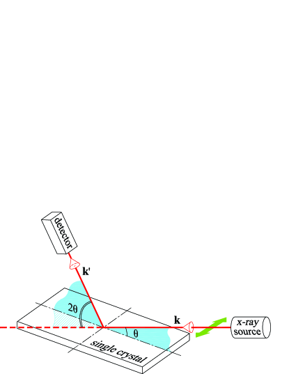
Figure 1: (Color online) Schematic drawing of the geometry for the K-edge RIXS experiment reported in this paper. The polarization direction is orthogonal to the scattering plane and is depicted with a green arrow.

We make further approximations to simplify the numerical calculation of RIXS spectrum. First, we replace the sum $\sum_{n^{\bf d}}$ by a single term with $n^{\bf d}=n^{\bf d}_{\rm low}$, that is, the lowest energy eigenstate with the core hole at a site ${\bf d}$. This is justified for two reasons: Ahn09 First, $\langle n^{\bf d}|\underline{s}_{\bf d}^{\dagger}|g\rangle$ is largest for $n^{\bf d}_{\rm low}$, the well-screened state. Second, the incoming x-ray energy is tuned to the absorption edge, which makes the lowest energy intermediate state the most probable, while higher energy intermediate states, in particular, the unscreened state, Ahn09 are less likely to be excited by the incoming x-rays in a K-edge RIXS process. The lowest energy intermediate state $|n^{\bf d}_{\rm low}\rangle$ is dominated by the single-pair electron-hole excitations, especially in insulators, because of the higher energies necessary for multiple-pair electron-hole excitations. Ahn09 We therefore consider single-pair final states $\langle l_{e}{\bf k}_{e}l_{h}{\bf k}_{h}\sigma|$ with an electron with wavevector ${\bf k}_{e}$, band index $l_{e}$, and energy $\varepsilon_{l_{e}{\bf k}_{e}}$ and a hole with wavevector ${\bf k}_{h}$, band index $l_{h}$, and energy $\varepsilon_{l_{h}{\bf k}_{h}}$, both with spin $\sigma$. Finally, if the resonant energies $E_{n^{\bf d}}-E_{g}$ and core-hole lifetime broadenings $\Gamma_{n^{\bf d}}$ are similar for different core-hole sites within the unit cell, then we can neglect the denominator in Eq. (2) for fixed incoming x-ray energy, because it becomes a constant factor in the overall K-edge RIXS spectrum. These approximations lead to the following formula, which we use for the numerical calculation of the K-edge RIXS spectrum.

$$I(\omega,{\bf Q})\propto$$

$$\sum_{\bf K}\sum_{l_{e}{\bf k}_{e}l_{h}{\bf k}_{h}\sigma}\left|\sum_{\bf d}e^{-i{\bf Q}\cdot{\bf d}}\langle l_{e}{\bf k}_{e}l_{h}{\bf k}_{h}\sigma|\underline{s}_{\bf d}|n^{\bf d}_{\rm low}\rangle\langle n^{\bf d}_{\rm low}|\underline{s}_{\bf d}^{\dagger}|g\rangle\right|^{2}\!\!\!\!\times$$

$$\delta(\varepsilon_{l_{h}{\bf k}_{h}}-\varepsilon_{l_{e}{\bf k}_{e}}+\hbar\omega)\ \delta({\bf k}_{e}-{\bf k}_{h}+{\bf Q}+{\bf K}),$$ (3)

where ${\bf Q}={\bf k}^{\prime}-{\bf k}$. This formula relates the K-edge RIXS spectrum to the response of the system to a localized charge. The reasonable approximations we have taken significantly reduce the time for numerical calculations, and therefore, this formula can be used with the density functional approach as well as the tight-binding approach. Details on how we numerically calculate $I(\omega,\bf{Q})$ with Eq. (3) are presented in Appendix B.

II.2 Periodicity of K-edge RIXS in reciprocal space

Understanding the periodicity of the K-edge RIXS spectrum is useful, for example, in determining where to probe in reciprocal space. Also, as we will show below, there is useful information in the momentum dependence. First, it should be noted that periodicity in reciprocal space is not inherent in inelastic x-ray scattering. For example, off resonance, an increase in transferred momentum changes the transition matrix elements, since higher order terms in the multipole expansion of the vector potential ${\bf A}$ are no longer negligible. Ament11 However, on resonance, the matrix elements are all in the dipole limit and should not depend on the momenta of the incoming and outgoing photons. The only relevant momentum is then the crystal momentum, and the K-edge RIXS cross section follows the symmetry of the Brillouin zone. This was noted experimentally by Kim et al. Kim07 in their study of high-T_c cuprates. However, these materials have only one transition metal site in the unit cell. Such periodicity may not be generally applicable to crystals with multiple core-hole sites within a unit cell, such as charge-orbital ordered manganites.

We look into the formula in Eq. (3) to learn about the periodicity of K-edge RIXS spectrum. For solid systems with one core-hole site per unit cell, we can choose ${\bf d}=0$ and simplify Eq. (3) by omitting a constant factor $\langle n^{\bf d}_{\rm low}|\underline{s}_{\bf d}^{\dagger}|g\rangle$ to obtain,

$$I(\omega,{\bf Q})\propto \sum_{\bf K}\sum_{l_{e}{\bf k}_{e}l_{h}{\bf k}_{h}\sigma}\left|\langle l_{e}{\bf k}_{e}l_{h}{\bf k}_{h}\sigma|\underline{s}_{{\bf d}=0}|n^{{\bf d}=0}_{\rm low}\rangle\right|^{2}\ \times$$ (4)

$$\delta(\varepsilon_{l_{h}{\bf k}_{h}}-\varepsilon_{l_{e}{\bf k}_{e}}+\hbar\omega)\ \delta({\bf k}_{e}-{\bf k}_{h}+{\bf Q}+{\bf K}),$$

which makes the RIXS calculations even simpler for materials with one core-hole site per unit cell. If the x-ray wavevector change ${\bf Q}$ is altered by a reciprocal lattice vector ${\bf K}^{\prime}$, i.e., ${\bf Q}^{\prime}={\bf Q}+{\bf K}^{\prime}$, then the RIXS intensity will be unchanged, since ${\bf K}^{\prime\prime}={\bf K}^{\prime}+{\bf K}$ in the second $\delta$-function is also a reciprocal lattice vector. This is consistent with the experimental result for La₂CuO₄ (Ref. Kim07, ).

On the other hand, if a solid has multiple core-hole sites per unit cell due to the ordering of spin, charge, orbital, or local lattice distortions, then the following argument shows that the symmetry of the K-edge RIXS spectrum is with respect to the lattice without ordering, rather than the actual lattice. We represent the lattice without ordering by ${\bf R}_{\rm core}$, which includes the actual lattice ${\bf R}$ as well as ${\bf d}$. Then ${\bf K}_{\rm core}$, the reciprocal lattice vector of ${\bf R}_{\rm core}$, satisfies the condition of $e^{i{\bf K}_{\rm core}\cdot{\bf d}}=1$, which results in the symmetry of K-edge RIXS spectrum in Eq. (3), that is, $I(\omega,{\bf Q}+{\bf K}_{\rm core})=I(\omega,{\bf Q})$. We shall see this explicitly in Sec. V.6 for La_0.5Sr_1.5MnO₄.

III Experimental results for La_0.5Sr_1.5MnO₄

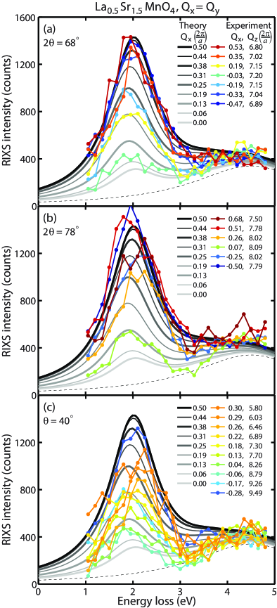
Figure 2: (Color online) Experimental and theoretical K-edge RIXS intensities for La_0.5Sr_1.5MnO₄ with CE-type charge-orbital-spin ordering. The symbols in panels (a), (b) and (c) represent the experimental data, taken at $2\theta=68^{\circ}$, $2\theta=78^{\circ}$, and $\theta=40^{\circ}$ respectively, and $Q_{x}=Q_{y}=H_{\rm ex}\frac{2\pi}{a}$ and $Q_{z}=L_{\rm ex}\frac{2\pi}{a}$. The elastic peaks are subtracted from data. Liu13 Dashed line represents a momentum-independent peak, presumably from a O-Mn transition. Solid curves in gray scale represent the RIXS intensity calculated at $Q_{x}=Q_{y}=H_{\rm th}\frac{2\pi}{a}$ for the Mn-Mn transition for the parameter set with $t_{0}$ = 0.9 eV, added to the dashed line, as discussed in Sec. V D.

Mn K-edge RIXS from La_0.5Sr_1.5MnO₄ was measured at the Advanced Photon Source on beamlines 30-ID and 9-ID at temperature $T$ = 20 K, well below CE-type magnetic, charge, orbital, and structural ordering temperatures. The instrumental energy resolution was of about 270 meV (FWHM). As shown in Fig. 1, a single crystal grown in traveling solvent floating zone method is aligned so that when the x-ray wavevector transfer ${\bf Q}$ is in the scattering plane, it has $Q_{x}=Q_{y}$ with the $x$ and $y$ axes along the Mn-O bond direction and the $z$ axis perpendicular to the MnO₂ plane. The scattering plane was fixed with respect to the crystal and the polarization of the incoming and outgoing x-rays was perpendicular to the scattering plane, so that the polarization factor is a constant factor in the RIXS formula, as assumed in the derivation of Eq. (3). Data taken either at a fixed sample angle, $\theta$, or a fixed detector angle, 2$\theta$, are shown as connected dots in Fig. 2. The elastic peak has been subtracted from the data. Liu13 The main focus in this paper is the intensity variation of the 2 eV peak, which is known to arise from transitions between Mn $3d$ $e_{g}$ bands from optical measurements. Ishikawa99 ; Jung00 The intensity of the 2 eV peak increases rapidly from $Q_{x}=Q_{y}=0$ to $Q_{x}=Q_{y}=\pm\frac{\pi}{a}$, where $a$ represent the average Mn-Mn distance within the MnO₂ plane, but is almost independent of $Q_{z}$. While the latter supports the two-dimensional character of the $e_{g}$ electrons confined within each MnO₂ layer, the former cannot be explained by dynamic structure factor $S({\bf q},\omega)$. This, combined with the fact that there are eight core-hole sites per two-dimensional unit cell, makes the experimental results for La_0.5Sr_1.5MnO₄ an ideal case to test the validity of our theory.

IV Tight binding Hartree-Fock Hamiltonian and core-hole potential for $e_{g}$ electrons in La_0.5Sr_1.5MnO₄

La_0.5Sr_1.5MnO₄ has a layered two-dimensional perovskite structure with negligible hopping of the Mn $3d$ $e_{g}$ electrons between the MnO₂ layers. This is consistent with the experimental observation of K-edge RIXS spectrum being independent of the momentum transfer perpendicular to MnO₂ layers. We therefore consider a Hamiltonian for a single MnO₂ layer. La_0.5Sr_1.5MnO₄ undergoes a structural and orbital ordering transition at 230 K, and a CE-type magnetic ordering transition at 110 K, schematically shown in Fig. 3 for the MnO₂ layer. In this figure, “Mn³⁺” and “Mn⁴⁺” are used to indicate the two sites not related by symmetry, rather than controversial charge ordering. Herrero04 ; Brey04 ; Coey04 The strong Hund’s coupling between the $e_{g}$ electron spin and the $t_{2g}$ electron spin confines most of the $e_{g}$ electron hopping along the zigzag chain. The distortion of the oxygen octahedron surrounding the Mn ions splits the $e_{g}$ energy levels through the Jahn-Teller electron-lattice coupling.

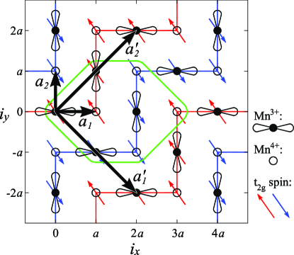
Figure 3: (Color online) In-plane structural layout of Mn ions for La_0.5Sr_1.5MnO₄ in CE-type ordering. Red and blue arrows represent the $t_{2g}$ spin alignment. ${\bf a}^{\prime}_{1}$ and ${\bf a}^{\prime}_{2}$ represent the primitive lattice vectors for CE-phase. ${\bf a}_{1}$ and ${\bf a}_{2}$ are primitive vectors for lattice without charge, orbital, and spin ordering. The rounded hexagon encloses the Mn ions in the basis.

Our tight-binding Hamiltonian considers the effective Mn $3d$ $e_{g}$ levels only, because the RIXS peak at around 2 eV is due to transitions between the bands from these levels. Ishikawa99 ; Jung00 We note that these effective Mn $3d$ $e_{g}$ levels are in fact linear combinations of atomic Mn $3d$ $e_{g}$ levels and atomic O $2p$ levels. Appendix D discusses this aspect in more detail, in particular, in relation to the electron numbers on the Mn ions.

Within this effective model, we define $d^{\dagger}_{{\bf i}\xi\sigma}$ as the creation operator of the $e_{g}$ electron with the spin state $\sigma$ = $\uparrow$, $\downarrow$ and orbital state $\xi=1$ for $(3z^{2}-r^{2})/2$ and $\xi=2$ for $\sqrt{3}(x^{2}-y^{2})/2$ at the Mn site ${\bf i}=(m_{x}a,m_{y}a)$, where $m_{x}$ and $m_{y}$ are integers, as shown in Fig. 3. The electron hopping term Ahn00 is

$$\hat{H}_{\rm hopping}=-\frac{1}{2}\sum_{{\bf i},\boldsymbol{\delta},\xi,\xi^{\prime},\sigma}\!\!\!t_{\boldsymbol{\delta}}^{\xi\xi^{\prime}}\left(d_{{\bf i}\xi\sigma}^{\dagger}d_{{\bf i}+\boldsymbol{\delta},\xi^{\prime},\sigma}+d_{{\bf i}+\boldsymbol{\delta},\xi^{\prime},\sigma}^{\dagger}d_{{\bf i}\xi\sigma}\right).$$ (5)

The vector $\boldsymbol{\delta}=\pm a\hat{x},\pm a\hat{y}$ represents the nearest neighbor sites of a Mn ion. The hopping matrices within the MnO₂ plane are

$$t_{a\hat{x}} = t_{-a\hat{x}}=t_{0}\left(\begin{array}[]{cc}1/4&-\sqrt{3}/4\\ -\sqrt{3}/4&3/4\end{array}\right),$$ (8)

$$t_{a\hat{y}} = t_{-a\hat{y}}=t_{0}\left(\begin{array}[]{cc}1/4&\sqrt{3}/4\\ \sqrt{3}/4&3/4\end{array}\right),$$ (11)

reflecting the symmetry of the $e_{g}$ orbitals. The parameter $t_{0}$ represents the effective hopping constant between the two $(3x^{2}-r^{2})/2$ orbitals along the $x$-direction.

The distortion of oxygen octahedron around a Mn ion at site ${\bf i}$ is parameterized as follows. $u_{\bf i}^{\zeta}$ ($\zeta$ = $x,y$) represents the $\hat{\zeta}$ directional displacement of an oxygen ion located between Mn ions at ${\bf i}$ and ${\bf i}+a\hat{\zeta}$ from the position for the ideal undistorted square MnO₂ lattice with the average in-plane Mn-O bond distance. The $u_{\bf i}^{+z}$ and $u_{\bf i}^{-z}$ represent the $z$ direction displacements of the oxygen ions above and below the Mn ion at site ${\bf i}$ from the location of the average in-plane Mn-O bond distance. The parameters, $Q_{1{\bf i}}$, $Q_{2{\bf i}}$, and $Q_{3{\bf i}}$, represent the distortion modes of the oxygen octahedron, shown in Fig. 4 and defined as follows.

$$Q_{1{\bf i}} = \frac{u^{x}_{\bf i}-u^{x}_{{\bf i}-a\hat{x}}+u^{y}_{\bf i}-u^{y}_{{\bf i}-a\hat{y}}+u^{+z}_{\bf i}-u^{-z}_{\bf i}}{\sqrt{3}},$$ (12)

$$Q_{2{\bf i}} = \frac{u^{x}_{\bf i}-u^{x}_{{\bf i}-a\hat{x}}-u^{y}_{\bf i}+u^{y}_{{\bf i}-a\hat{y}}}{\sqrt{2}},$$ (13)

$$Q_{3{\bf i}} = \frac{2u^{z}_{\bf i}-2u^{-z}_{\bf i}-u^{x}_{\bf i}+u^{x}_{{\bf i}-a\hat{x}}-u^{y}_{\bf i}+u^{y}_{{\bf i}-a\hat{y}}}{\sqrt{6}}.$$ (14)

The Mn-O bond distances estimated from structural refinement of high-resolution synchrotron x-ray powder diffraction data for La_0.5Sr_1.5MnO₄ in Ref. Herrero11, indicate $Q_{1}=0.0531$ Å, $Q_{2}=\pm 0.1089$ Å, and $Q_{3}=0.0955$ Å around the “Mn³⁺” sites and $Q_{1}=-0.0531$ Å, $Q_{2}=0$, and $Q_{3}=0.1192$ Å around the “Mn⁴⁺” sites.

Figure 4: Distortion modes $Q_{1}$, $Q_{2}$, and $Q_{3}$ of oxygen octahedron around Mn with arrows indicating directions of displacement.

The $Q_{2}$ and $Q_{3}$ distortions break the cubic symmetry of the oxygen octahedra and interact with the $e_{g}$ orbital state through the following Jahn-Teller Hamiltonian term, note-JT

$$\hat{H}_{\rm JT}=-\lambda\sum_{{\bf i},\sigma}\left(\begin{array}[]{c}d_{{\bf i}1\sigma}^{\dagger}\\ d_{{\bf i}2\sigma}^{\dagger}\end{array}\right)^{T}\left(\begin{array}[]{cc}Q_{3{\bf i}}&-Q_{2{\bf i}}\\ -Q_{2{\bf i}}&-Q_{3{\bf i}}\end{array}\right)\left(\begin{array}[]{c}d_{{\bf i}1\sigma}\\ d_{{\bf i}2\sigma}\end{array}\right),$$ (15)

where $\lambda$ corresponds to the Jahn-Teller coupling constant. The isotropic $Q_{1}$ distortion interacts with the total $e_{g}$ electron number through the following “breathing” electron-lattice Hamiltonian term, Millis96

$$\hat{H}_{\rm br}=-\beta\lambda\sum_{{\bf i},\sigma}\left(\begin{array}[]{c}d_{{\bf i}1\sigma}^{\dagger}\\ d_{{\bf i}2\sigma}^{\dagger}\end{array}\right)^{T}\left(\begin{array}[]{cc}Q_{1{\bf i}}&0\\ 0&Q_{1{\bf i}}\end{array}\right)\left(\begin{array}[]{c}d_{{\bf i}1\sigma}\\ d_{{\bf i}2\sigma}\end{array}\right),$$ (16)

where $\beta$ represents the ratio between the strengths of the breathing and the Jahn-Teller coupling.

We also include the Hund’s coupling of the $e_{g}$ electron spin state to the classical $t_{2g}$ spin direction,

$$\hat{H}_{\rm Hund}=-J_{H}\sum_{{\bf i},\xi,\sigma^{\prime},\sigma^{\prime\prime}}{\bf S}_{t_{2g}{\bf i}}\cdot d_{{\bf i}\xi\sigma^{\prime}}^{\dagger}\ \boldsymbol{\tau}_{\sigma^{\prime}\sigma^{\prime\prime}}\ d_{{\bf i}\xi\sigma^{\prime\prime}},$$ (17)

where $J_{H}$ represents the Hund’s coupling constant, ${\bf S}_{t_{2g}{\bf i}}$ the $t_{2g}$ spin vector ordered in CE-type structure and $\boldsymbol{\tau}$ is the Pauli matrix vector.

As in Ref. Ahn00, , we also include the $3d$-$3d$ on-site Coulomb interaction,

$$\hat{H}_{\rm dd}=U\sum_{\bf i}\sum_{(\eta,\sigma)\neq(\eta^{\prime},\sigma^{\prime})}\hat{n}_{{\bf i}\eta\sigma}\hat{n}_{{\bf i}\eta^{\prime}\sigma^{\prime}},$$ (18)

where $\hat{n}_{{\bf i}\eta\sigma}=d^{{\dagger}}_{{\bf i}\eta\sigma}d_{{\bf i}\eta\sigma}$ is the number operator and $U$ represents the size of the $3d$-$3d$ Coulomb interaction. The index $\eta=-,+$ represents the local orbital eigenstates of $\hat{H}_{\rm JT}$ with lower and higher energies, respectively, chosen for the following Hartree-Fock approximation:

$$\hat{H}_{\rm dd}^{\rm HF}=\sum_{\bf i}\bigg{(}U_{{\bf i}+\uparrow}d_{{\bf i}+\uparrow}^{\dagger}d_{{\bf i}+\uparrow}+U_{{\bf i}-\uparrow}d_{{\bf i}-\uparrow}^{\dagger}d_{{\bf i}-\uparrow}$$

$$+U_{{\bf i}+\downarrow}d_{{\bf i}+\downarrow}^{\dagger}d_{{\bf i}+\downarrow}+U_{{\bf i}-\downarrow}d_{{\bf i}-\downarrow}^{\dagger}d_{{\bf i}-\downarrow}\bigg{)},$$ (19)

where $U_{{\bf i}+\uparrow}=U(\langle\hat{n}_{{\bf i}-\uparrow}\rangle+\langle\hat{n}_{{\bf i}+\downarrow}\rangle+\langle\hat{n}_{{\bf i}-\downarrow}\rangle)$, etc. Ahn00

The total Hamiltonian for Mn $3d$ $e_{g}$ electrons for calculations of K-edge RIXS initial and final states is then the sum of the terms described so far,

$$\hat{H}_{\rm d}=\hat{H}_{\rm hopping}+\hat{H}_{\rm JT}+\hat{H}_{\rm br}+\hat{H}_{\rm Hund}+\hat{H}_{\rm dd}^{\rm HF}.$$ (20)

The CE type ordering of the $t_{2g}$ spins and the lattice distortions associated with charge and orbital ordering give rise to the primitive lattice vectors ${\bf a}^{\prime}_{1}$ and ${\bf a}^{\prime}_{2}$ shown in Fig. 3. The primitive reciprocal lattice vectors are ${\bf b}^{\prime}_{1}=(\frac{\pi}{2a},-\frac{\pi}{2a})$ and ${\bf b}^{\prime}_{2}=(\frac{\pi}{2a},\frac{\pi}{2a})$, and the first Brillouin zone is $\Omega_{\rm 1BZ}=\{{\bf k}|-\frac{\pi}{2a}<k_{x}+k_{y}\leq\frac{\pi}{2a}$, $-\frac{\pi}{2a}<k_{x}-k_{y}\leq\frac{\pi}{2a}\}$.

In the intermediate state, we must also account for the presence of the core hole. The $1s$-$3d$ on-site Coulomb interaction is generally expressed as

$$\hat{H}_{{\rm sd}}=-U_{\rm core}\sum_{{\bf i},\xi,\sigma,\sigma^{\prime}}d^{\dagger}_{{\bf i}\xi\sigma}\ d_{{\bf i}\xi\sigma}\ \underline{s}^{\dagger}_{{\bf i}\sigma^{\prime}}\ \underline{s}_{{\bf i}\sigma^{\prime}},$$ (21)

where $U_{\rm core}$ represents the size of the $1s$-$3d$ Coulomb interaction, and $\underline{s}^{\dagger}_{{\bf i}\sigma^{\prime}}$ is the creation operator for a $1s$ core hole with spin $\sigma^{\prime}$ at site ${\bf i}$. As discussed in Sec. II.1, in the limit of vanishing $1s$ electron hopping amplitude, the K-edge RIXS intermediate energy eigenstates can be chosen as states with a single completely localized $1s$ core hole, which can be found from

$$\hat{H}_{{\rm total},{\bf i}_{c}}=\hat{H}_{\rm d}+\hat{H}_{{\rm sd},{\bf i}_{c}},$$ (22)

with

$$\hat{H}_{{\rm sd},{\bf i}_{c}}=-U_{\rm core}\sum_{\xi,\sigma}d^{\dagger}_{{\bf i}_{c}\xi\sigma}\ d_{{\bf i}_{c}\xi\sigma},$$ (23)

${\bf i}_{c}$ representing the $1s$ core-hole site, and $\underline{s}^{\dagger}_{{\bf i}_{c}\sigma^{\prime}}\ \underline{s}_{{\bf i}_{c}\sigma^{\prime}}=1$ being used. To calculate the K-edge RIXS spectrum, we need to represent the eigenstates of $\hat{H}_{{\rm total},{\bf i}_{c}}$, as a linear combination of the eigenstates of $\hat{H}_{\rm d}$, as described in detail in Appendix B. The expression of the Hamiltonian $\hat{H}_{\rm d}$ and $\hat{H}_{{\rm total},{\bf i}_{c}}$ in reciprocal space for La_0.5Sr_1.5MnO₄ is presented in Appendix C.

Each Hamiltonian term has one parameter. Some of the parameter values are chosen by modifying corresponding values for LaMnO₃ found in Ref. Ahn00, . The chosen parameter values are $t_{0}$ = 0.9 eV, $\lambda$ = 7.41 eV/Å, $\beta$ = 1.5, $J_{H}|{\bf S}_{t_{2g},{\bf i}}|$ = 2.2 eV, $U$ = 3.5 eV, and $U_{\rm core}$ = 4.0 eV. In addition, we vary $t_{0}$ and $\lambda$ while maintaining the gap size around 2 eV to examine how the RIXS spectrum depends on the $e_{g}$ electron hopping amplitude.

V Results from theory and comparison with experiments

V.1 Electronic density of states in the absence and in the presence of the core hole

We first present our results on energy eigenstates and eigenvalues of the Hamiltonians for a 16$\times$16 Mn site cluster with periodic boundary conditions. The calculated density of states (DOS) is shown in Fig. 5(a) in the absence of a core hole. The occupied band mostly consists of the lower Jahn-Teller $e_{g}$ levels with spin parallel to the $t_{2g}$ spins at Mn³⁺ sites, whereas the lowest empty band mostly consists of similar $e_{g}$ levels at Mn⁴⁺ sites. The excitation between these two bands is responsible for the 2 eV RIXS peak, which is the focus of our comparison with experiment data. Due to spin degeneracy in CE-type antiferromagnetic ordering, the electronic DOS $D_{\downarrow}(\varepsilon)$ for spin $\downarrow$, is identical to that for spin $\uparrow$, $D_{\uparrow}(\varepsilon)$.

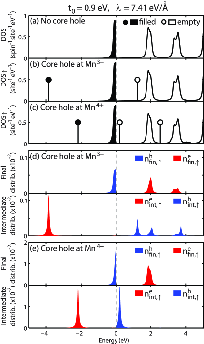
Figure 5: (Color online) Electronic density of states (DOS) per site, for $t_{0}=0.9$ eV and $\lambda=7.41$ eV/Å (a) without a core hole, (b) with a core hole at a Mn³⁺ site and (c) with a core hole at a Mn⁴⁺ site. The Lorentzian broadening of 2$\Gamma$ = 0.1 eV is used to make the DOS curve smooth. Vertical lines with a circle on top represent bound states. (d) and (e): Final (upper panel) and intermediate (lower panel) electron-hole distribution with a core hole at a (d) Mn³⁺ and (e) Mn⁴⁺ site.

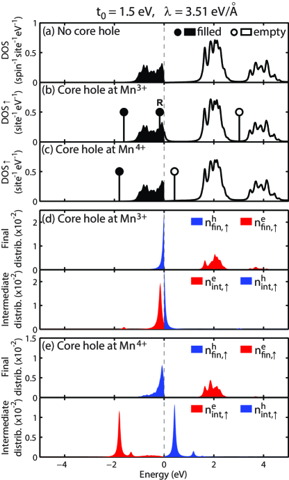
Figure 6: (Color online) Similar figures as Fig. 5 for $t_{0}=1.5$ eV and $\lambda=3.51$ eV/Å. “R” in (b) represents a resonant state, rather than a bound state. Note that a single state at the top of the lower band in (b) is empty.

We next analyze the Hamiltonian $\hat{H}_{{\rm total},{\bf i}_{c}}$ in the presence of the core hole at site ${\bf i}_{c}$. The $t_{2g}$ spin direction at ${\bf i}_{c}$ breaks the spin degeneracy in the DOS. The DOS $D_{\uparrow}^{{\bf i}_{c}=(0,0)}(\varepsilon)$ is displayed in Fig. 5(b), for the core hole site ${\bf i}_{c}=(0,0)$ in Fig. 3, which is a Mn³⁺ site with $t_{2g}$ spin $\uparrow$. The core-hole potential pulls out bound states from the band continuum, Ahn09 identified by vertical lines with circles on top in Fig. 5(b). The lowest bound state is at about $-4$ eV, that is, $U_{\rm core}$ below the lowest band with Mn³⁺ character. The second bound state is within the gap. The DOS for the band continuum is almost unchanged, except that the number of states within each band below and above the gap is reduced by one because of the bound states pulled out. Ahn09 By filling the states from the lowest energy with the same number of electrons in the intermediate states as in the ground state, as shown in Fig. 5(b), we obtain the lowest energy intermediate state, $\underline{s}|n_{\rm low}^{{\bf i}_{c}}\rangle$. Therefore, the bound state below the lowest band is occupied and the bound state within the gap is empty in the intermediate state. $D_{\downarrow}^{{\bf i}_{c}=(0,0)}(\varepsilon)$ is almost identical to the DOS without a core hole in Fig. 5(a), because the electrons with spin $\downarrow$ contribute very little to the screening of the core hole due to the strong Hund’s coupling.

The DOS $D_{\uparrow}^{{\bf i}_{c}=(a,0)}(\varepsilon)$, for the core hole at ${\bf i}_{c}=(a,0)$ in Fig. 3, which is a Mn⁴⁺ site with $t_{2g}$ spin $\uparrow$, is shown in Fig. 5(c) and has similar features. The lowest bound state is at around $-2$ eV, that is, $U_{\rm core}$ below the band with the Mn⁴⁺ site character, which is the lowest empty band. Again, the lowest bound state is filled and the bound state within the gap is empty for $\underline{s}|n_{\rm low}^{{\bf i}_{c}}\rangle$, as indicated in Fig. 5(c).

As a comparison, we carry out similar calculations for the parameter values of $t_{0}$ = 1.5 eV and $\lambda$ = 3.51 eV/Å, which keep the size of the gap approximately 2 eV, but result in a larger band width. Due to the larger electron hopping, the gap has more of a hybridization gap character, and the bands are wider, as shown in Fig. 6(a), which shows the DOS without a core hole. Similarly to the $t_{0}$ = 0.9 eV case, Figs. 6(b) and 6(c) show $D_{\uparrow}^{{\bf i}_{c}}(\varepsilon)$, in the presence of a core hole at ${\bf i}_{c}=(0,0)$ and ${\bf i}_{c}=(a,0)$, respectively. The bound states in Fig. 6(c) are qualitatively similar to those for $t_{0}$ = 0.9 eV in Fig. 5(c). However, qualitatively different behavior occurs for the core hole at a Mn³⁺ site, as shown in Fig. 6(b). In this case, the bound state that would be in the gap for smaller $t_{0}$ resides in the occupied band and becomes a resonant rather than bound state, as indicated by the vertical line with “R” on top. Such a resonant state hybridizes with delocalized states in the band, unlike bound states. With the bound state below the lower band and this resonant state occupied, the top of the lower band is empty in the lowest energy intermediate state $\underline{s}|n_{\rm low}^{{\bf i}_{c}}\rangle$, as indicated in Fig. 6(b). This will have a significant consequence in the screening dynamics, as discussed in following sections.

V.2 Electron and hole excitations by the core hole represented along energy axis

Understanding the distributions of the electrons and holes that are excited by the core hole is essential for the interpretation of RIXS spectrum. Excited electron and hole distributions with respect to the energy for the RIXS final state, $n_{{\rm fin},\sigma}^{e}(\varepsilon)$ with $\varepsilon>\varepsilon_{F}$ and $n_{{\rm fin},\sigma}^{h}(\varepsilon)$ with $\varepsilon<\varepsilon_{F}$, are defined as follows Ahn09

$$n_{{\rm fin},\sigma}^{e}(\varepsilon) = \!\!\!\!\!\sum_{l{\bf k}}^{\varepsilon_{l{\bf k}\sigma}>\varepsilon_{F}}\sum_{m=1}^{\frac{N_{e}}{2}}\left|\langle 0|b_{l{\bf k}\sigma}c_{m\sigma}^{\dagger}|0\rangle\right|^{2}\delta(\varepsilon-\varepsilon_{l{\bf k}\sigma}),$$ (24)

$$n_{{\rm fin},\sigma}^{h}(\varepsilon) = \!\!\!\!\!\sum_{l{\bf k}}^{\varepsilon_{l{\bf k}\sigma}<\varepsilon_{F}}\!\!\!\!\!\sum_{m=\frac{N_{e}}{2}+1}^{\frac{N_{e}}{2}}\!\!\!\!\!\left|\langle 0|b_{l{\bf k}\sigma}c_{m\sigma}^{\dagger}|0\rangle\right|^{2}\delta(\varepsilon-\varepsilon_{l{\bf k}\sigma}),$$ (25)

where $\varepsilon_{F}$ represents the Fermi energy in the absence of the core hole, $c_{m\sigma}^{\dagger}$ is the creation operator for the $m$-th lowest energy eigenstate of $\hat{H}_{{\rm total},{\bf i}_{c}}$ with spin $\sigma$ and energy $\varepsilon_{m\sigma}$, and $b_{l{\bf k}\sigma}^{\dagger}$ represents the creation operator for the energy eigenstate with wavevector ${\bf k}$ and energy $\varepsilon_{l{\bf k}\sigma}$ within the $l$-th lowest band of $\hat{H}_{\rm d}$, and $N_{e}$ represents total electron number. These are the electrons and holes that are moved by the scattering process. For example, $n_{\rm fin}^{e}(\varepsilon)$ corresponds to the projection of occupied intermediate states to unoccupied initial states. The $\delta$-function makes this distribution represented with respect to the energy without the core hole.

Similar electron and hole distributions with respect to the energy for the RIXS intermediate state, Ahn09 $n_{{\rm int},\sigma}^{e}(\varepsilon)$ and $n_{{\rm int},\sigma}^{h}(\varepsilon)$, are defined in the same way as Eqs. (24) and (25), except that the energy $\delta$-function is replaced by $\delta(\varepsilon-\varepsilon_{m\sigma})$. This difference also implies that we have $n_{{\rm int},\sigma}^{e}(\varepsilon)$ for $\varepsilon<\varepsilon_{F}^{\rm int}$ and $n_{{\rm int},\sigma}^{h}(\varepsilon)$ for $\varepsilon>\varepsilon_{F}^{\rm int}$, where $\varepsilon_{F}^{\rm int}$ represents the Fermi energy in the presence of the core hole.

These excited electron and hole distributions are plotted in Figs. 5(d), 5(e), 6(d), and 6(e) for $\sigma$ = $\uparrow$. Similar distributions for spin $\downarrow$ state are less than 10% of those for spin $\uparrow$ state. The plots of $n^{e}_{\rm int,\uparrow}(\varepsilon)$ and $n^{h}_{\rm int,\uparrow}(\varepsilon)$ in the lower panels of Figs. 5(d), 5(e), and 6(e) show that the bound states in the intermediate state, marked in Fig. 5(b), 5(c), and 6(c), respectively, make the dominant contribution to the electron-hole excitations.

The plots of $n^{h}_{\rm fin,\uparrow}(\varepsilon)$ and $n^{e}_{\rm fin,\uparrow}(\varepsilon)$ in the upper panels of Figs. 5(d), 5(e) and 6(e), show that, while $n_{{\rm fin},\sigma}^{e}(\varepsilon)$ resembles the DOS of the unoccupied band, $n_{{\rm fin},\sigma}^{h}(\varepsilon)$ shows a peak at the top of the occupied band, in particular, in Fig. 6(e). This represents asymmetric screening dynamics between electrons and holes.

For the exceptional case of $t_{0}$ = 1.5 eV and a core hole at Mn³⁺ site, the comparison between Fig. 6(b) and the lower panel in Fig. 6(d) reveals that the occupied resonant state within the lower band marked by “R” and the empty state at the top of the occupied band in Fig. 6(b) make dominant contributions to $n^{e}_{\rm int,\uparrow}(\varepsilon)$ and $n^{h}_{\rm int,\uparrow}(\varepsilon)$. The resonant state is dominant for electron excitations because this state is pulled from the initially unoccupied bands, whereas the lowest bound state comes mostly from the initially occupied band. The delocalized state at the top of the occupied band predominantly contributes to the hole excitation, because it is occupied in the initial state and empty in the intermediate state, which results in hole excitation very close to the gap shown in the upper panel in Fig. 6(d).

We note that these results are consistent with the conclusions of Ref. Ahn09, , thus validating the present study.

V.3 Electron and hole excitations by the core hole represented in real space

In this subsection, we present the distribution of electrons and holes excited by the core hole in real space.

First, in the absence of the core hole, the electron number $\langle\hat{n}_{{\bf i}\eta\sigma}\rangle$ is calculated for each spin state $\sigma=\uparrow,\downarrow$ and orbital state $\eta=+,-$ at each site ${\bf i}$ from the initial ground state $|g\rangle$ of the Hamiltonian $\hat{H}_{\rm d}$. The total $e_{g}$ electron numbers calculated for our $16\times 16$ cluster in the absence of the core hole are 0.87 at the nominal Mn³⁺ site and 0.13 at the nominal Mn⁴⁺ site for the parameter set with $t_{0}$ = 0.9 eV, indicating a difference of 0.74 in charge density between these two sites. We note that these numbers should not be directly compared with the local density approximation theory results or resonant x-ray scattering results, because our effective Mn $3d$ $e_{g}$ states are not pure atomic Mn orbital states but combinations of atomic Mn and O orbitals. Herrero10 A proper comparison is described in Appendix D, which shows that the electron numbers in our model are consistent with local density approximation and resonant x-ray scattering results. It is found that most of these electrons occupy the lower Jahn-Teller level $\eta=-$, approximately $\sqrt{3}(x^{2}-z^{2})/2$ or $\sqrt{3}(y^{2}-z^{2})/2$ orbital at the Mn³⁺ site and the $(3z^{2}-r^{2})/2$ orbital at the Mn⁴⁺ site, with spin parallel to $t_{2g}$ spin at each site, consistent with the orbital ordering proposed in Ref. Zeng08, .

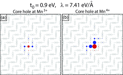
Figure 7: (Color online) Screening configuration in real space for $t_{0}=0.9$ eV with a core hole at a (a) Mn³⁺, and (b) Mn⁴⁺ site. The volume of the red and blue spheres is proportional to the excited electron and hole numbers, respectively. The excited electron number at the core-hole site (the site with the largest red sphere) is 0.11 for (a) and 0.92 for (b).

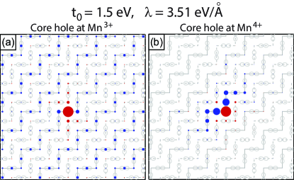
Figure 8: (Color online) Screening configuration in real space for $t_{0}=1.5$ eV with a core hole at a (a) Mn³⁺, and (b) Mn⁴⁺ site, similar to Fig. 7. The excited electron number at the core-hole site is 1.02 for (a) and 0.91 for (b).

In the intermediate state, these electron numbers change to screen the core hole. The changes in electron number, that is, excited electron and hole numbers, are shown in Fig. 7 for $t_{0}$ = 0.9 eV and in Fig. 8 for $t_{0}$ = 1.5 eV, where the volumes of red and blue spheres are proportional to the excited electron and hole numbers, respectively. Note that these changes in electron and hole numbers are consistent with the excited electron and hole distributions along the energy axis reported in Figs. 5(d), 5(e), 6(d) and 6(e). The site with the largest electron number in each panel corresponds to the core-hole site. The gray solid and dashed lines in the background represent the zigzag chain with $t_{2g}$ spin $\uparrow$ and $\downarrow$, respectively. For the $t_{0}$ = 0.9 eV case, Figs. 7(a) and 7(b) show that the excited electrons are mostly confined right at the core-hole site. The localization of the electrons in the intermediate state leads to the relatively broad electron distribution, $n^{e}_{\rm fin\uparrow}(\varepsilon)$, along the energy axis in the upper panels of Figs. 5(d) and 5(e). Comparison of the largest solid red spheres in Figs. 7(a) and 7(b) shows that more screening electrons accumulate at the core-hole site when the core hole is created at the Mn⁴⁺ site (0.92 electron) than at the Mn³⁺ (0.11 electron). This result can be understood from the orbital ordering pattern: Initially, the Mn⁴⁺ site has less $e_{g}$ electrons on the site itself but more electrons at its nearest neighbor Mn sites along the zigzag chain with orbitals pointing toward the Mn⁴⁺ site compared to the Mn³⁺ site, which allows the core hole at Mn⁴⁺ sites to attract more electrons. Hole distribution in Figs. 7(a) and 7(b) show that these screening electrons are mostly from the nearest neighbors along the zigzag chain, accounting for about 90% of the total hole number. The results show that even though the hole excitation is not as localized as the electron excitation and $n^{h}_{\rm fin\uparrow}(\varepsilon)$ is sharper along the energy axis than $n^{e}_{\rm fin\uparrow}(\varepsilon)$ in Fig. 5(d) and 5(e), the holes are still tightly bound to the core-hole site forming an exciton-like electron-hole-pair state.

The situation changes for the case of large electron hopping $t_{0}$ = 1.5 eV. Figure 8(a) shows the electron-hole excitations for a core hole at a Mn³⁺ site. In this case, the hole distribution becomes delocalized, and only about 8% of the hole is localized within the nearest neighbors of the core-hole site, while the majority of the hole is delocalized along the zigzag chains with the same spin direction as the core-hole site, consistent with the result in Figs. 6(b) and 6(d). The hole number does not decay with the distance from the core-hole site, indicating qualitatively different screening dynamics. Even for the case with a core hole at a Mn⁴⁺ site, Fig. 8(b), the hole distribution spreads to further neighbors along the zig-zag chain, reflecting the tendency toward delocalization.

As we shall see, such screening patterns in real space can be related to the variation of the RIXS intensity in reciprocal space. This will be discussed in Sec. V.5.

V.4 Calculated K-edge RIXS spectrum and comparison with experimental data

We calculate the RIXS intensity, $I(\omega,{\bf Q})$ according to Eq. (3). To make a comparison between the calculated results and the experimental data, we first examine the experimental data more closely. In addition to the momentum-dependent RIXS peak at around 2 eV, the experimental RIXS spectrum in Fig. 2 shows momentum-independent spectral weight, in particular above 3 eV. The shape of the experimental RIXS spectrum, particularly with small in-plane wavevector changes, such as $Q_{x}=Q_{y}=-0.03\times\frac{2\pi}{a}$ in Fig. 2(a), indicates that the RIXS spectral weight above 3 eV may have the same origin as the 4–5 eV O $2p$-Mn $3d$ transition observed in optical experiments in related manganites.Jung00 Based on this assumption, we model the experimental RIXS spectrum with a momentum-independent peak, shown in dashed lines in Fig. 2, centered at 4.5 eV and with a half-width at half-maximum of 1.5 eV similar to the optical peak, and a momentum-dependent Mn $3d$-$3d$ peak around 2 eV, calculated from Eq. (3) using $\hat{H}_{\rm d}$ and $\hat{H}_{{\rm total},{\bf i}_{c}}$. Here, although it does not affect the results much, we use the RIXS intensity averaged over twin domains in the crystal with zigzag chains along the [$110$] and [$\bar{1}10$] directions, $I_{\rm avg}(\omega,(Q_{x},Q_{y}))=[I(\omega,(Q_{x},Q_{y}))+I(\omega,(-Q_{x},Q_{y}))]/2$. The results in Fig. 2 demonstrate a reasonable agreement between the calculated spectra shown in solid lines and the experimental data shown in symbols, considering the experimental noise. The 4.5 eV peak has a substantial tail even in the range of 1–3 eV. Such momentum-independent tails have also been observed in bilayer manganites. Weber10

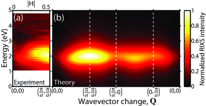
Figure 9: (Color online) (a) Experimental RIXS intensity. Here we take experimental data of Fig. 2, subtract the 4.5 eV peak, and fit the resulting data with a fifth order polynomial, which is plotted as a contour plot. (b) Contour plot of the calculated RIXS intensity for the $t_{0}=0.9$ eV case along the chosen path in reciprocal space.

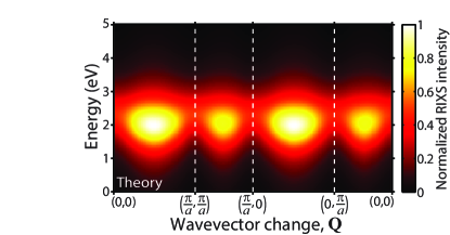
Figure 10: (Color online) Contour plot of the calculated RIXS intensity for $t_{0}=1.5$ eV along the chosen path in reciprocal space.

To compare just the 2 eV peak between the theory and experiment, we subtract the 4.5 eV peak from the experimental data and plot the intensity, as a contour plot in the plane of energy and $Q_{x}=Q_{y}=H_{\rm ex}\frac{2\pi}{a}$ in Fig. 9(a). This clearly shows the momentum dependence of the intensity of the 2 eV peak. The calculated RIXS intensity in Fig. 9(b) for $t_{0}$ = 0.9 eV shows good agreement with experimental data. In contrast, in Fig. 10, we show the calculated RIXS spectrum for $t_{0}$ = 1.5 eV, which is not consistent with the experimental data.

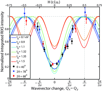
Figure 11: (Color online) K-edge RIXS intensity integrated from 1 to 3 eV as a function of wavevector change, normalized with respect to the maximum. Symbols with error bars represent experimental data. Lines represent the results from the theory, for several $t_{0}$ cases for comparison.

V.5 Energy-integrated RIXS intensity in reciprocal space

To make a more quantitative comparison between theory and experiment, we integrate the spectrum of the 2 eV peak from 1 eV to 3 eV after subtracting 4.5 eV peak, for both theory and experiment. The results are shown in Fig. 11 along the diagonal direction in reciprocal space, in which the theoretical results for the various parameter sets, and the experimental data are normalized with respect to the maximum integrated intensity. The parameter sets used for the calculations are $(t_{0},\lambda)$ = (0.1 eV, 10.79 eV/Å), (0.9 eV, 7.41 eV/Å), (1.1 eV, 4.81 eV/Å), (1.32 eV, 3.76 eV/Å), (1.35 eV, 3.73 eV/Å), and (1.50 eV, 3.51 eV/Å), chosen to keep the peak at around 2 eV. All other parameter values are unchanged. The experimental data in Fig. 11 shows that the integrated RIXS intensity increases 4–5 times as the wavevector ${\bf Q}$ varies from ${\bf Q}=(0,0)$ to ${\bf Q}=(\frac{\pi}{a},\frac{\pi}{a})$. Considering fluctuations in experimental data, the theoretical results for $t_{0}$ = 0.1, 0.9, 1.1 eV, all of which have exciton-like screening electron-hole excitations similar to Fig. 7, fit the experimental data reasonably well. In contrast, the theoretical results for $t_{0}$ = 1.35 and 1.5 eV, all of which have delocalized hole excitations similar to Fig. 8, are qualitatively different from experimental data with maximum intensity at around $(\pm\frac{\pi}{2a},\pm\frac{\pi}{2a})$ instead of $(\pm\frac{\pi}{a},\pm\frac{\pi}{a})$. This provides an upper limit of about 1.2 eV for the value of $t_{0}$.

This analysis indicates that, irrespective of the details of the model Hamiltonian and the particular parameter values, the rapid increase of the RIXS intensity with a maximum at $(\pm\frac{\pi}{a},\pm\frac{\pi}{a})$ observed in the experiment is indicative of highly localized screening dynamics note-PiPi in La_0.5Sr_1.5MnO₄, i.e., screening that is more like Fig. 7 than that of Fig. 8.

V.6 Periodicity of K-edge RIXS spectrum in reciprocal space for charge-orbital-spin ordered manganites

As mentioned in Sec. II.2, in earlier studies of La₂CuO₄, it was shown that the observed K-edge RIXS spectrum reflects the periodicity of the lattice and is a function of the reduced wavevector ${\bf q}$ within the first Brillouin zone, defined as ${\bf Q}={\bf q}+{\bf K}$, where ${\bf Q}$ is the total x-ray wavevector change and ${\bf K}$ is a reciprocal lattice vector. Kim07

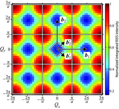
Figure 12: (Color online) K-edge RIXS intensity integrated from 1 eV to 3 eV, shown in a large reciprocal space for the $t_{0}=0.9$ eV case. ${\bf b}^{\prime}_{1}$ and ${\bf b}^{\prime}_{2}$ represent the primitive reciprocal lattice vectors of charge-orbital-spin ordered MnO₂ plane of Fig. 3. ${\bf b}_{1}$ and ${\bf b}_{2}$ are the primitive reciprocal lattice vectors for MnO₂ lattice without ordering.

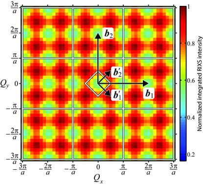
Figure 13: (Color online) Similar figure as Fig. 12 for the $t_{0}=1.5$ eV case.

The experimental data presented in this paper clearly indicates that such periodicity is not present for La_0.5Sr_1.5MnO₄. The measured RIXS intensity, as well as the calculated RIXS intensity, seen in Figs. 9 and 11, increases continuously past the boundary of the first Brillouin zone at $(\frac{\pi}{4a},\frac{\pi}{4a})$. As discussed in Sec. II.2, the periodicity seen in Ref. Kim07, applies only to solids with one core-hole site per unit cell, such as La₂CuO₄. For solids with multiple core hole sites per unit cell due to the ordering of spin, charge, orbital or local lattice distortions, the periodicity in K-edge RIXS spectrum follows the periodicity of the lattice without ordering, like the square Mn-site lattice in La_0.5Sr_1.5MnO₄, not the periodicity of the actual lattice with ordering. Our numerical calculations in Figs. 12 and 13 confirm such periodicity in La_0.5Sr_1.5MnO₄: Fig. 12 shows energy-integrated RIXS intensity calculated for the $t_{0}$ = 0.9 eV case in a larger region of reciprocal space of $-\frac{3\pi}{a}<Q_{x}\leq\frac{3\pi}{a}$ and $-\frac{3\pi}{a}<Q_{y}\leq\frac{3\pi}{a}$. The diamond around $(0,0)$ is the actual first Brillouin zone of the spin, charge and orbital ordered structure, whereas the outer square domain $-\frac{\pi}{a}<Q_{x}\leq\frac{\pi}{a}$ and $-\frac{\pi}{a}<Q_{y}\leq\frac{\pi}{a}$, denotes the first Brillouin zone of the lattice without ordering. It is evident that RIXS spectrum does not exhibit periodicity with respect to the actual primitive reciprocal lattice vectors, ${\bf b}^{\prime}_{1}$ and ${\bf b}^{\prime}_{2}$, shown in Fig. 12, but rather shows periodicity with respect to primitive reciprocal lattice vectors of the lattice without ordering, ${\bf b}_{1}$ and ${\bf b}_{2}$, shown in Fig. 12. Even though it is only a single data point, the experimental data at around $Q_{x}=Q_{y}=0.68\times\frac{2\pi}{a}$ in Fig. 11 is consistent with such periodicity. Further experimental data for $|Q_{x}|>\frac{\pi}{a}$, $|Q_{y}|>\frac{\pi}{a}$ are required for the verification of this periodicity. We note that careful examination of Fig. 12 reveals that the periodicity is only approximate. The small displacement of the Mn⁴⁺ ions of 0.0265 Å along the diagonal direction from the ideal square lattice, Zeng08 included in our calculations, makes the Mn sites deviate slightly from the exact square lattice. Figure 13 shows that, even for the $t_{0}$ = 1.5 eV case, the periodicity still does not follow the actual reciprocal lattice, even though the RIXS intensity oscillates more rapidly in reciprocal space.

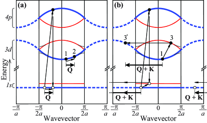
Figure 14: (Color online) Schematic diagrams of a band structure of a one-dimensional system with a lattice constant $a$, before [thick (blue) lines, both solid and dashed] and after [solid lines, both thick (blue) and thin (red)] artificial unit cell doubling. The thin black dotted lines in the $3d$ bands represent the modification of the band structure after real unit cell doubling due to charge-orbital ordering. Panels (a) and (b) represent the RIXS processes that result in x-ray wavevector transfers of ${\bf Q}$ and ${\bf Q+K}$, respectively, with ${\bf K}=-\frac{\pi}{a}$, a reciprocal lattice vector for the lattice with the doubled unit cell.

We next provide a physical explanation of why the K-edge RIXS spectrum from charge-orbital ordered manganites follows the periodicity of the Brillouin zone in the absence of charge-orbital order. We first consider artificial doubling of the unit cell for a one-dimensional chain with interatomic distance $a$. In Fig. 14, thick (blue) lines, both solid and dashed, and solid lines, both thick (blue) and thin (red), show a schematic diagram of the band structure before and after the artificial unit cell doubling, respectively. The arrows between $1s$ and $4p$ bands represent the core hole creation and annihilation by x-rays. Due to the interaction with the core-hole, electron-hole pairs can be excited into the valence shell, as indicated by the arrows within the $3d$ band. Excitations with a transferred crystal wavevector ${\bf Q}$ from the state $1$ can be either an intraband transition to the state $2$ shown in Fig. 14(a) or an interband transition to the state 3 shown in Fig. 14(b). However, the reduced Brillouin zone $[-\frac{\pi}{2a},\frac{\pi}{2a}]$ is an artificial construction and should give equivalent results to the real Brillouin zone $[-\frac{\pi}{a},\frac{\pi}{a}]$, in which the state $3^{\prime}$ in Fig. 14(b) should be considered instead of the state $3$. Therefore, the intraband and interband transitions correspond to wavevector transfers of ${\bf Q}$ and ${\bf Q+K}$, respectively, where ${\bf K}$ is $-\frac{\pi}{a}$, a reciprocal lattice vector of the doubled unit cell. This implies that they occur at two distinct wavevector transfers and should be distinguishable. The underlying reason is that not only the valence bands are backfolded due to the doubling of unit cell, but also the core level bands. An interband (intraband) transition in the valence band also leads to an interband (intraband) transition in the core level band, as shown in arrows in the $1s$ band in Fig. 14. We now consider real unit cell doubling due to charge-orbital order. For a finite but small charge-orbital order, the band structure would be modified mostly near the Brillouin zone boundary, as represented by the thin black dotted lines in the $3d$ bands in Fig. 14, and the RIXS that involves states far from the zone boundary, such as the states $1$, $2$ and $3$, should not dramatically change from those in the absence of charge-orbital order. Therefore, the K-edge RIXS spectrum $I(\omega,{\bf Q})$ and $I(\omega,{\bf Q+K})$ would remain different even after charge-orbital ordering. Obviously, the situation becomes more complex when the charge-orbital order becomes stronger leading to a further mixing of the bands. However, the schematic figure explains why the periodicity for charge-orbital ordered manganites occurs with the Brillouin zone in the absence of such order.

VI Discussion

In this section, we discuss what insights the RIXS spectrum in reciprocal space can provide on the screening dynamics. Figures 15(a) and 15(b) show $n_{h}/n_{h}^{\max}$, that is the hole density normalised to its maximum, versus distance $l$ from the core-hole site along the zig-zag chain for the case of core hole at a Mn³⁺ and Mn⁴⁺ site, respectively, in a semi-logarithmic plot. For $t_{0}\leq 1.3$ eV of Fig. 15(a) and all $t_{0}$ of Fig. 15(b), the hole density decreases exponentially and thus can be fit to $n_{h}/n_{h}^{\max}\propto\exp(-l/l_{s})$, where $l_{s}$ can be interpreted as the size of the screening cloud. We find that the sizes of the screening clouds are approximately $0.4$ and $0.5$ interatomic distances for the Mn³⁺ and Mn⁴⁺ sites, respectively, for $t_{0}$ = 0.9 eV, and become larger, as $t_{0}$ increases, as shown along the horizontal axis in Fig. 15(c), which includes the result for $t_{0}=0.6$ eV additionally.

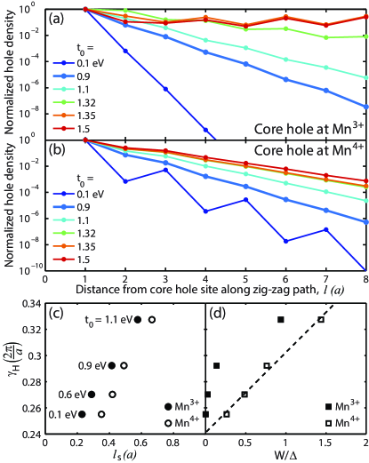
Figure 15: (Color online) (a) and (b): Semi-log plot of the excited hole number normalized to its maximum versus the distance from the core-hole site for a Mn³⁺, and a Mn⁴⁺ core hole site, respectively. (c) The width of the RIXS peak at $(\pm\frac{\pi}{a},\pm\frac{\pi}{a})$ in reciprocal space, $\gamma_{H}$, found from Fig. 11, versus screening cloud size in real space $l_{s}$, found from (a) and (b), for various $t_{0}$ values. (d) $\gamma_{\rm H}$ versus the ratio between the occupied band width $(W)$ and the in-gap bound state energy $(\Delta)$ from the occupied band edge, $W/\Delta$.

We next look for a correlation between the size of the screening cloud in real space and the features of the K-edge RIXS spectrum in reciprocal space. We define $\gamma_{H}$ as the half-width-at-half-maximum in reciprocal space of the energy-integrated RIXS peak for $t_{0}\leq 1.3$ eV in Fig. 11. The plot of $\gamma_{H}$ versus $l_{s}$ is displayed in Fig. 15(c), which shows a linear correlation. Therefore, the width of the energy-integrated RIXS peak in reciprocal space in Fig. 11 can be used to estimate the size of the screening hole cloud. This is an important result with general implications.

The size of the screening hole cloud depends on the competition between hole hopping and hole binding energies, which can be parameterized in terms of $W$, the width of the occupied band, and $\Delta$, the energy difference between the top of the occupied band and the unoccupied bound state within the gap, or, the hole binding energy. Therefore, from the connection between $l_{s}$ and $\gamma_{H}$ established above, we examine whether the width of the RIXS peak $\gamma_{H}$ can also provide insight on the ratio $W/\Delta$. The $\gamma_{H}$ versus $W/\Delta$ plot in Fig. 15(d) confirms a positive correlation between these quantities, in particular a linear correlation for the case of core hole at Mn⁴⁺ site. The results indicate that the width of the RIXS peak can be a measure of the size of the exciton-like screening cloud in real space, and a measure of the ratio between the occupied band width and the hole binding energy.

Recently, K-edge RIXS spectra for bilayer manganites La_2-2xSr_1+2xMn₂O₇ with $x$ = 0.36 and 0.5 have been reported by Weber et al. Weber10 Although not as pronounced as our results for single layered manganites, Ref. Weber10, shows an increase of the 2 eV peak intensity in A-type and CE-type antiferromagnetic LaSr₂Mn₂O₇, as the x-ray wavevector transfer increases from $(0,0,Q_{z})$ to $(\frac{\pi}{a},\frac{\pi}{a},Q_{z})$. In the context of our work above, such results can be interpreted as the formation of an exciton-like screening cloud in bi-layer manganites, the size of which is likely larger than that for the single-layer manganites discussed above, considering the less-pronounced increase of the 2 eV peak intensity.

Finally, we note that Semba et al. calculated the K-edge RIXS spectrum for LaMnO₃, based on the Keldysh-type Green’s function formalism.Semba08 The results in Ref. Semba08, show about a 10% increase of the 2 eV peak from $(0,0,0)$ to $(1,0,0)$ in their choice of $x$ and $y$ axes, which are equivalent to ${\bf Q}=(0,0,0)$ to ${\bf Q}=(\frac{\pi}{a},\frac{\pi}{a},0)$ in our notation. The results again can be interpreted as the formation of exciton-like screening clouds, consistent with our calculations, even though the core-hole state for the intermediate eigenstates is chosen as delocalised in Ref. Semba08, . The periodicity of the RIXS spectrum discussed in Sec. II.2 and Sec. V.6 was also identified in Ref. Semba08, , even though the association of such periodicity with the approximate square lattice of the core-hole sites was not specifically mentioned.

VII Summary

We have presented a formalism to calculate the K-edge RIXS spectra in transition metal oxides based on tight-binding Hamiltonians and a local $1s$–$3d$ Coulomb interaction, in which the choice of intermediate eigenstates with a completely localized $1s$ core hole allows for the interpretation of the data in terms of screening dynamics in real space. We have also found that the periodicity of K-edge RIXS spectrum follows the reciprocal lattice vectors of the lattice without the ordering of spin, charge, orbital, or local lattice distortions, rather than the reciprocal lattice vectors of the actual lattice with such ordering.

We have applied our formalism to the highly-momentum-dependent K-edge RIXS spectrum observed for La_0.5Sr_1.5MnO₄ in CE-type spin-orbital-structure ordering. It is found that the sharp increase of the 2 eV peak intensity from the center toward the corner of the first Brillouin zone of the lattice without ordering is an indication of a highly localized screening cloud in La_0.5Sr_1.5MnO₄ with a typical size of 0.4–0.5 Mn-Mn distances. We also showed that there exists a positive correlation between the width of the energy-integrated K-edge RIXS intensity peak in reciprocal space, the size of the exciton-like screening cloud in real space, and the ratio between occupied band width and hole binding energy.

The analysis in this paper was performed for the case of an intermediate strength core-hole potential, that is $U_{\rm core}$ comparable to the $3d$ electron bandwidth. In fact, this is appropriate for most transition metal oxides and therefore the present approach should have general applicability. One of the important results is that this approach highlights the connection between K-edge RIXS and the impurity problem in strongly correlated electron systems, and we show that this technique is a new probe of momentum-dependent screening dynamics of localized impurities.

Appendix A RIXS formula derivation

As explained in Sec. II.1, we get the following formula from the Kramers-Heisenberg formula, Eq. (1), in the limit of completely localized core hole,

$$I(\omega,{\bf k},{\bf k}^{\prime},\boldsymbol{\epsilon},\boldsymbol{\epsilon}^{\prime})\propto$$

$$\sum_{f}\left|\sum_{\bf R}\sum_{\bf d}\sum_{n^{{\bf R}+{\bf d}}}\frac{\langle f|\mathcal{D^{\prime}}^{{\dagger}}|n^{{\bf R}+{\bf d}}\rangle\langle n^{{\bf R}+{\bf d}}|\mathcal{D}|g\rangle}{E_{g}+\hbar\omega_{\bf k}-E_{n^{\bf d}}+i\Gamma_{n^{\bf d}}}\right|^{2}\times$$

$$\delta(E_{g}-E_{f}+\hbar\omega),$$ (26)

where $|n^{{\bf R}+{\bf d}}\rangle$ represents the intermediate energy eigenstate with the core hole at a site ${\bf R}+{\bf d}$ within the unit cell at a lattice point ${\bf R}$. Further applying the dipole approximation to the K-edge scattering amplitude, we obtain

$$\langle f|\mathcal{D^{\prime}}^{{\dagger}}|n^{{\bf R}+{\bf d}}\rangle\langle n^{{\bf R}+{\bf d}}|\mathcal{D}|g\rangle=e^{-i({\bf k}^{\prime}-{\bf k})\cdot({\bf R}+{\bf d})}\times$$

$$\boldsymbol{\epsilon}^{\prime}\cdot\langle f|{\bf r}|n^{{\bf R}+{\bf d}}\rangle\ \ \boldsymbol{\epsilon}\cdot\langle n^{{\bf R}+{\bf d}}|{\bf r}|g\rangle.$$ (27)

Two many-body states $|\Psi^{0}\rangle$ and $|\Psi^{{\bf R}}\rangle$, which have total momentum $\hbar\boldsymbol{\kappa}$ and identical wave functions in two different coordinate systems with the coordinates for $|\Psi^{{\bf R}}\rangle$ shifted with respect to the coordinates for $|\Psi^{0}\rangle$ by ${\bf R}$, are related to each other by a phase factor $|\Psi^{{\bf R}}\rangle$ = $e^{-i\boldsymbol{\kappa}\cdot{\bf R}}|\Psi^{0}\rangle$. Assuming that $|g\rangle$ and $|f\rangle$ have net momenta of zero and $\hbar{\bf k}_{f}$, respectively, we obtain the following relation, note-R

$$\langle f|{\bf r}|n^{{\bf R}+{\bf d}}\rangle = e^{-i{\bf k}_{f}\cdot{\bf R}}\langle f|{\bf r}|n^{\bf d}\rangle,$$ (28)

$$\langle n^{{\bf R}+{\bf d}}|{\bf r}|g\rangle = \langle n^{\bf d}|{\bf r}|g\rangle.$$ (29)

Therefore, the sum over lattice vectors ${\bf R}$ for the combined factor of $e^{-i({\bf k}^{\prime}-{\bf k}+{\bf k}_{f})\cdot{\bf R}}$ from Eqs. (27)–(29) leads to the conservation of the crystal momentum $\delta({\bf k}^{\prime}-{\bf k}+{\bf k}_{f}+{\bf K})$, where ${\bf K}$ represents the reciprocal lattice vectors. This results in the following expression for the RIXS intensity,

$$I(\omega,{\bf k},{\bf k}^{\prime},\boldsymbol{\epsilon},\boldsymbol{\epsilon}^{\prime})\propto\sum_{\bf K}\sum_{f}\left|\sum_{\bf d}\sum_{n^{\bf d}}\frac{e^{-i({\bf k}^{\prime}-{\bf k})\cdot{\bf d}}\ \boldsymbol{\epsilon}^{\prime}\cdot\langle f|{\bf r}|n^{\bf d}\rangle\;\boldsymbol{\epsilon}\cdot\langle n^{\bf d}|{\bf r}|g\rangle}{E_{g}+\hbar\omega_{\bf k}-E_{n^{\bf d}}+i\Gamma_{n^{\bf d}}}\right|^{2}\delta(E_{f}+\hbar\omega_{{\bf k}^{\prime}}-E_{g}-\hbar\omega_{\bf k})\ \delta({\bf k}_{f}+{{\bf k}^{\prime}}-{\bf k}+{\bf K}).$$ (30)

By further assuming special experimental setups in which the polarization vectors $\boldsymbol{\epsilon}^{\prime}$ and $\boldsymbol{\epsilon}$ give rise to a constant factor, as mentioned in Sec. II.1, and neglecting a constant factor from the dipole moment between $4p$ and $1s$ wave functions, we obtain Eq. (2) in Sec. II.1.

Appendix B Expression of the matrix elements in the K-edge RIXS formula in terms of eigenstates in the presence and absence of core hole

In general, we transform $\hat{H}_{\rm d}$ and $\hat{H}_{{\rm total},{\bf i}_{c}}$ into the reciprocal space as follows,

$$\hat{H}_{\rm d}=\sum_{{\bf k},{\bf k}^{\prime}}\sum_{{\bf K},{\bf K}^{\prime}}\sum_{\xi,\xi^{\prime}}\sum_{\sigma} H^{\rm d}_{{\bf k}+{\bf K},\xi,{\bf k}^{\prime}+{\bf K}^{\prime},\xi^{\prime},\sigma}\ \times$$ (31)

$$d_{{\bf k}+{\bf K},\xi,\sigma}^{{\dagger}}d_{{\bf k}^{\prime}+{\bf K}^{\prime},\xi^{\prime},\sigma},$$

and

$$\hat{H}_{{\rm total},{\bf i}_{c}}=\sum_{{\bf k},{\bf k}^{\prime}}\sum_{{\bf K},{\bf K}^{\prime}}\sum_{\xi,\xi^{\prime}}\sum_{\sigma} H^{{\rm total},{\bf i}_{c}}_{{\bf k}+{\bf K},\xi,{\bf k}^{\prime}+{\bf K}^{\prime},\xi^{\prime},\sigma}\ \times$$ (32)

$$d_{{\bf k}+{\bf K},\xi,\sigma}^{{\dagger}}d_{{\bf k}^{\prime}+{\bf K}^{\prime},\xi^{\prime},\sigma},$$

where ${\bf k}$ and ${\bf k}^{\prime}$ represent vectors within the first Brillouin zone $\Omega_{\rm 1BZ}$, ${\bf K}$ and ${\bf K}^{\prime}$ the reciprocal lattice vectors within the extended “first Brillouin zone” $\Omega_{\rm ExZ}$ defined by the core hole site ${\bf i}$. Spin states are represented by $\sigma$, and orbital states by $\xi$ and $\xi^{\prime}$.

From the eigenstates $|l{\bf k}\sigma\rangle$ of $\hat{H}_{\rm d}$ with the wavevector ${\bf k}\in\Omega_{\rm 1BZ}$ within the $l$-th lowest energy band, and the $m$-th lowest energy eigenstate $|m\sigma\rangle$ of $\hat{H}_{{\rm total},{\bf i}_{c}}$, we define $\beta_{l{\bf k}m\sigma}$ = $\langle l{\bf k}\sigma|m\sigma\rangle$.

In the RIXS formula Eq. (3), $\langle n^{\bf d}_{\rm low}|\underline{s}_{\bf d}^{\dagger}|g\rangle$ and $\langle l_{e}{\bf k}_{e}l_{h}{\bf k}_{h}\sigma|\underline{s}_{\bf d}|n^{\bf d}_{\rm low}\rangle$ are found from

$$\langle n^{\bf d}_{\rm low}|\underline{s}_{\bf d}^{\dagger}|g\rangle=\prod_{\sigma=\uparrow\downarrow}\left|\begin{array}[]{cccc}\beta_{1{\bf k}_{1}1\sigma}&\beta_{1{\bf k}_{1}2\sigma}&\cdots&\beta_{1{\bf k}_{1}\frac{N_{e}}{2}\sigma}\\ \beta_{1{\bf k}_{2}1\sigma}&\beta_{1{\bf k}_{2}2\sigma}&\cdots&\beta_{1{\bf k}_{2}\frac{N_{e}}{2}\sigma}\\ \vdots&\vdots&\ddots&\vdots\\ \beta_{l_{h}^{\rm max}{\bf k}_{N_{k}}1\sigma}&\beta_{l_{h}^{\rm max}{\bf k}_{N_{k}}2\sigma}&\cdots&\beta_{l_{h}^{\rm max}{\bf k}_{N_{k}}\frac{N_{e}}{2}\sigma}\end{array}\right|,$$ (33)

$$\langle l_{e}{\bf k}_{e}l_{h}{\bf k}_{h}\sigma|\underline{s}_{\bf d}|n^{\bf d}_{\rm low}\rangle=\left|\begin{array}[]{cccc}\beta_{1{\bf k}_{1}1\sigma}&\beta_{1{\bf k}_{1}2\sigma}&\cdots&\beta_{1{\bf k}_{1}\frac{N_{e}}{2}\sigma}\\ \beta_{1{\bf k}_{2}1\sigma}&\beta_{1{\bf k}_{2}2\sigma}&\cdots&\beta_{\sigma 1{\bf k}_{2}\frac{N_{e}}{2}}\\ \vdots&\vdots&\ddots&\vdots\\ \beta_{l_{h}^{\prime\prime}{\bf k}_{h}^{\prime\prime}1\sigma}&\beta_{l_{h}^{\prime\prime}{\bf k}_{h}^{\prime\prime}2\sigma}&\cdots&\beta_{l_{h}^{\prime\prime}{\bf k}_{h}^{\prime\prime}\frac{N_{e}}{2}\sigma}\\ \beta_{l_{e}{\bf k}_{e}1\sigma}&\beta_{l_{e}{\bf k}_{e}2\sigma}&\cdots&\beta_{l_{e}{\bf k}_{e}\frac{N_{e}}{2}\sigma}\\ \beta_{l_{h}^{\prime\prime\prime}{\bf k}_{h}^{\prime\prime\prime}1\sigma}&\beta_{l_{h}^{\prime\prime\prime}{\bf k}_{h}^{\prime\prime\prime}2\sigma}&\cdots&\beta_{l_{h}^{\prime\prime\prime}{\bf k}_{h}^{\prime\prime\prime}\frac{N_{e}}{2}\sigma}\\ \vdots&\vdots&\ddots&\vdots\\ \beta_{l_{h}^{\rm max}{\bf k}_{N_{k}}1\sigma}&\beta_{l_{h}^{\rm max}{\bf k}_{N_{k}}2\sigma}&\cdots&\beta_{l_{h}^{\rm max}{\bf k}_{N_{k}}\frac{N_{e}}{2}\sigma}\end{array}\right|\times\left|\begin{array}[]{cccc}\beta_{1{\bf k}_{1}1\bar{\sigma}}&\beta_{1{\bf k}_{1}2\bar{\sigma}}&\cdots&\beta_{1{\bf k}_{1}\frac{N_{e}}{2}\bar{\sigma}}\\ \beta_{1{\bf k}_{2}1\bar{\sigma}}&\beta_{1{\bf k}_{2}2\bar{\sigma}}&\cdots&\beta_{1{\bf k}_{2}\frac{N_{e}}{2}\bar{\sigma}}\\ \vdots&\vdots&\ddots&\vdots\\ \beta_{l_{h}^{\rm max}{\bf k}_{N_{k}}1\bar{\sigma}}&\beta_{l_{h}^{\rm max}{\bf k}_{N_{k}}2\bar{\sigma}}&\cdots&\beta_{l_{h}^{\rm max}{\bf k}_{N_{k}}\frac{N_{e}}{2}\bar{\sigma}}\end{array}\right|$$ (34)

where $N_{e}$ represents the total electron number, $N_{k}$ the number of ${\bf k}$-points in $\Omega_{\rm 1BZ}$, $l_{h}^{\rm max}$ the index for the highest occupied band, and $\bar{\sigma}=-\sigma$. In Eq. (34), the set of band and momentum indices, ($l_{h}^{\prime\prime}$, ${\bf k}_{h}^{\prime\prime}$) and ($l_{h}^{\prime\prime\prime}$, ${\bf k}_{h}^{\prime\prime\prime}$), represent the occupied states right before and right after the hole state represented by ($l_{h}$, ${\bf k}_{h}$) when the eigenstates of $\hat{H}_{\rm d}$ are ordered according to the band index and momentum index. note-beta

Appendix C Expressions of the Hamiltonians in reciprocal space with and without a $1s$ core hole for La_0.5Sr_1.5MnO₄

In the absence of the core hole, the Hamiltonian for a single layer of La_0.5Sr_1.5MnO₄ has the following form in reciprocal space,

$$\hat{H}_{\rm d}=\sum_{\sigma,{\bf k}\in\Omega_{\rm 1BZ}}d^{\dagger}_{{\bf k}\sigma}\left(H^{\rm d,nonint}_{{\bf k}\sigma}+H^{\rm dd,HF}_{{\bf k}\sigma}\right)d_{{\bf k}\sigma},$$ (35)

where

$$d^{\dagger}_{{\bf k}\sigma} = (d^{\dagger}_{{\bf k}+{\bf K}_{1},1,\sigma},d^{\dagger}_{{\bf k}+{\bf K}_{1},2,\sigma},d^{\dagger}_{{\bf k}+{\bf K}_{2},1,\sigma},d^{\dagger}_{{\bf k}+{\bf K}_{2},2,\sigma},d^{\dagger}_{{\bf k}+{\bf K}_{3},1,\sigma},d^{\dagger}_{{\bf k}+{\bf K}_{3},2,\sigma},d^{\dagger}_{{\bf k}+{\bf K}_{4},1,\sigma},d^{\dagger}_{{\bf k}+{\bf K}_{4},2,\sigma},$$ (36)

$$d^{\dagger}_{{\bf k}+{\bf K}_{5},1,\sigma},d^{\dagger}_{{\bf k}+{\bf K}_{5},2,\sigma},d^{\dagger}_{{\bf k}+{\bf K}_{6},1,\sigma},d^{\dagger}_{{\bf k}+{\bf K}_{6},2,\sigma},d^{\dagger}_{{\bf k}+{\bf K}_{7},1,\sigma},d^{\dagger}_{{\bf k}+{\bf K}_{7},2,\sigma},d^{\dagger}_{{\bf k}+{\bf K}_{8},1,\sigma},d^{\dagger}_{{\bf k}+{\bf K}_{8},2,\sigma})$$

with ${\bf K}_{1}$, ${\bf K}_{2}$, ${\bf K}_{3}$, ${\bf K}_{4}$, ${\bf K}_{5}$, ${\bf K}_{6}$, ${\bf K}_{7}$, and ${\bf K}_{8}$ representing $(0,0)$, $(\frac{\pi}{a},0)$, $(0,\frac{\pi}{a})$, $(\frac{\pi}{a},\frac{\pi}{a})$, $(-\frac{\pi}{2a},-\frac{\pi}{2a})$, $(\frac{\pi}{2a},-\frac{\pi}{2a})$ , $(-\frac{\pi}{2a},\frac{\pi}{2a})$, and $(\frac{\pi}{2a},\frac{\pi}{2a})$, respectively,

$$H^{\rm d,nonint}_{{\bf k}\sigma}=\left(\begin{array}[]{cccccccc}M_{1}+W_{3u}&-G_{\sigma}&G_{\sigma}&W_{1s}+W_{3s}&W_{2s}&G_{\sigma}&G_{\sigma}&W_{2s}\\ -G_{\sigma}&M_{2}+W_{3u}&W_{1s}+W_{3s}&G_{\sigma}&G_{\sigma}&W_{2s}&W_{2s}&G_{\sigma}\\ G_{\sigma}&W_{1s}+W_{3s}&M_{3}+W_{3u}&-G_{\sigma}&G_{\sigma}&W_{2s}&W_{2s}&G_{\sigma}\\ W_{1s}+W_{3s}&G_{\sigma}&-G_{\sigma}&M_{4}+W_{3u}&W_{2s}&G_{\sigma}&G_{\sigma}&W_{2s}\\ W_{2s}&G_{\sigma}&G_{\sigma}&W_{2s}&M_{5}+W_{3u}&-G_{\sigma}&G_{\sigma}&W_{1s}+W_{3s}\\ G_{\sigma}&W_{2s}&W_{2s}&G_{\sigma}&-G_{\sigma}&M_{6}+W_{3u}&W_{1s}+W_{3s}&G_{\sigma}\\ G_{\sigma}&W_{2s}&W_{2s}&G_{\sigma}&G_{\sigma}&W_{1s}+W_{3s}&M_{7}+W_{3u}&-G_{\sigma}\\ W_{2s}&G_{\sigma}&G_{\sigma}&W_{2s}&W_{1s}+W_{3s}&G_{\sigma}&-G_{\sigma}&M_{8}+W_{3u}\end{array}\right),$$ (37)

$$M_{j}=\left(\begin{array}[]{cc}-\dfrac{t_{0}}{2}[\cos(k_{x}+K_{j,x})+\cos(k_{y}+K_{j,y})]&\dfrac{\sqrt{3}t_{0}}{2}[\cos(k_{x}+K_{j,x})-\cos(k_{y}+K_{j,y})]\\ \dfrac{\sqrt{3}t_{0}}{2}[\cos(k_{x}+K_{j,x})-\cos(k_{y}+K_{j,y})]&-\dfrac{3t_{0}}{2}[\cos(k_{x}+K_{j,x})+\cos(k_{y}+K_{j,y})]\end{array}\right),$$ (38)

$$G_{\uparrow} = \left(\begin{array}[]{cc}-J_{H}S_{c}/2&0\\ 0&-J_{H}S_{c}/2\end{array}\right),$$ (41)

$$G_{\downarrow} = \left(\begin{array}[]{cc}J_{H}S_{c}/2&0\\ 0&J_{H}S_{c}/2\end{array}\right),$$ (44)

$$W_{\rm 1s} = \left(\begin{array}[]{cc}-\beta\lambda Q_{\rm 1s}&0\\ 0&-\beta\lambda Q_{\rm 1s}\end{array}\right),$$ (47)

$$W_{\rm 2s} = \left(\begin{array}[]{cc}0&\lambda Q_{\rm 2s}\\ \lambda Q_{\rm 2s}&0\end{array}\right),$$ (50)

$$W_{\rm 3u} = \left(\begin{array}[]{cc}-\lambda Q_{\rm 3u}&0\\ 0&\lambda Q_{\rm 3u}\end{array}\right),$$ (53)

$$W_{\rm 3s} = \left(\begin{array}[]{cc}-\lambda Q_{\rm 3s}&0\\ 0&\lambda Q_{\rm 3s}\end{array}\right),$$ (56)

$Q_{\rm 1s}=0.053$ Å, $Q_{\rm 2s}=0.054$ Å, $Q_{\rm 3u}=0.107$ Å, and $Q_{\rm 3s}=-0.012$ Å (Ref. Herrero11, ). The element of the $16\times 16$ matrix $H^{\rm dd,HF}_{{\bf k}\sigma}$ is independent of ${\bf k}$,

$$\left(H^{\rm dd,HF}_{{\bf k}\sigma}\right)_{2(j-1)+\xi,2(j^{\prime}-1)+\xi^{\prime}}=$$

$$\sum_{{\bf i}_{u},\eta}\frac{U_{{\bf i}_{u}\eta\sigma}}{8}e^{-i({\bf K}_{j}-{\bf K}_{j^{\prime}})\cdot{\bf i}_{u}}\left(R_{{\bf i}_{u}\eta}\right)_{\xi\xi^{\prime}}$$ (57)

where $\eta=+,-$, $j,j^{\prime}=1,2,\ldots,8$, and $\xi,\xi^{\prime}=1,2$. Further, ${\bf i}_{u}$ represents the position of the Mn ions within the unit cell, that is, $(0,0)$, $(a,0)$, $(2a,0)$, $(3a,0)$, $(a,-a)$, $(2a,-a)$, $(a,a)$, and $(2a,a)$ in Fig. 3, and

$$R_{{\bf i}_{u}-} = \left(\begin{array}[]{cc}\cos^{2}\theta_{{\bf i}_{u}}&\cos\theta_{{\bf i}_{u}}\sin\theta_{{\bf i}_{u}}\\ \cos\theta_{{\bf i}_{u}}\sin\theta_{{\bf i}_{u}}&\sin^{2}\theta_{{\bf i}_{u}}\end{array}\right),$$ (60)

$$R_{{\bf i}_{u}+} = \left(\begin{array}[]{cc}\sin^{2}\theta_{{\bf i}_{u}}&-\cos\theta_{{\bf i}_{u}}\sin\theta_{{\bf i}_{u}}\\ -\cos\theta_{{\bf i}_{u}}\sin\theta_{{\bf i}_{u}}&\cos^{2}\theta_{{\bf i}_{u}}\end{array}\right).$$ (63)

$\theta_{\bf i}$ is defined from the local lower ($-$) and upper ($+$) Jahn-Teller eigenstate,

$$d^{{\dagger}}_{{\bf i}-\sigma} = d^{{\dagger}}_{{\bf i}1\sigma}\cos\theta_{\bf i}+d^{{\dagger}}_{{\bf i}2\sigma}\sin\theta_{\bf i},$$ (64)

$$d^{{\dagger}}_{{\bf i}+\sigma} = -d^{{\dagger}}_{{\bf i}1\sigma}\sin\theta_{\bf i}+d^{{\dagger}}_{{\bf i}2\sigma}\cos\theta_{\bf i}.$$ (65)

At Mn³⁺ sites in the $x/y$ directional legs of the zigzag chain in Fig. 3,

$$\tan\theta_{\bf i}=\pm\frac{Q_{\rm 3u}+Q_{\rm 3s}-\sqrt{(Q_{\rm 3u}+Q_{\rm 3s})^{2}+4Q_{\rm 2s}^{2}}}{2Q_{\rm 2s}}$$ (66)

At Mn⁴⁺ sites, $\theta_{\bf i}=0$. The matrix for the number operator in reciprocal space is necessary to evaluate $U_{{\bf i}_{u}\eta\sigma}$ and its element is given below.

$$\left(n^{{\bf i}_{u}\eta\sigma}_{\bf k}\right)_{2(j-1)+\xi,2(j^{\prime}-1)+\xi^{\prime}}=e^{-i({\bf K}_{j}-{\bf K}_{j^{\prime}})\cdot{\bf i}_{u}}\left(R_{{\bf i}_{u}\eta}\right)_{\xi\xi^{\prime}}$$ (67)

We find the eigenstates and eigenenergies of the $16\times 16$ matrix $H^{\rm d}_{{\bf k}\sigma}=H^{\rm d,nonint}_{{\bf k}\sigma}+H^{\rm dd,HF}_{{\bf k}\sigma}$ at chosen set of ${\bf k}$ points through the Hartree-Fock iterative calculations, which are used to find the electronic DOS in the absence of the core hole shown in Figs. 5(a) and 6(a).

The Hamiltonian in the presence of the core hole at a site ${\bf i}_{c}$ for $N\times N$ cluster model of La_0.5Sr_1.5MnO₄, with $N$ multiple of 4, is presented below.

$$\hat{H}_{{\rm total},{\bf i}_{c}}=\sum_{\sigma,\ {\bf k},{\bf k}^{\prime}\in\Omega_{\rm 1BZ}} d^{\dagger}_{{\bf k}\sigma}\big{(}H^{\rm d,nonint}_{{\bf k}\sigma}\delta_{{\bf k}{\bf k}^{\prime}}+H^{\rm dd,HF}_{{\bf k}{\bf k}^{\prime}\sigma}$$ (68)

$$+H^{\rm sd,{\bf i}_{c}}_{{\bf k}{\bf k}^{\prime}\sigma}\big{)}\ d_{{\bf k}^{\prime}\sigma},$$

where

$$\left(H^{\rm dd,HF}_{{\bf k}{\bf k}^{\prime}\sigma}\right)_{2(j-1)+\xi,2(j^{\prime}-1)+\xi^{\prime}}=$$

$$\sum_{{\bf i},\eta}\frac{U_{{\bf i}\eta\sigma}}{N^{2}}\ e^{-i({\bf k}-{\bf k}^{\prime})\cdot{\bf i}}\ e^{-i({\bf K}_{j}-{\bf K}_{j^{\prime}})\cdot{\bf i}}\left(R_{{\bf i}\eta}\right)_{\xi\xi^{\prime}},$$ (69)

$$\left(H^{{\rm sd},{\bf i}_{c}}_{{\bf k}{\bf k}^{\prime}\sigma}\right)_{2(j-1)+\xi,2(j^{\prime}-1)+\xi^{\prime}}=$$

$$U_{\rm core}\ e^{-i({\bf k}-{\bf k}^{\prime})\cdot{\bf i}_{c}}\ e^{-i({\bf K}_{j}-{\bf K}_{j^{\prime}})\cdot{\bf i}_{c}}\ \delta_{\xi\xi^{\prime}},$$ (70)

with $\eta=+,-$, $\quad j,j^{\prime}=1,2,\ldots,8$, and $\xi,\xi^{\prime}=1,2$. For the evaluation of $U_{{\bf i}\eta\sigma}$, the number operator in receiprocal space is necessary, shown below.

$$\hat{n}^{{\bf i}\eta\sigma}=\sum_{{\bf k},{\bf k}^{\prime}\in\Omega_{\rm 1BZ}}d^{\dagger}_{{\bf k}\sigma}\ n^{{\bf i}\eta\sigma}_{{\bf k}{\bf k}^{\prime}}\ d_{{\bf k}^{\prime}\sigma},$$ (71)

where

$$\left(n^{{\bf i}\eta\sigma}_{{\bf k}{\bf k}^{\prime}}\right)_{2(j-1)+\xi,2(j^{\prime}-1)+\xi^{\prime}}=$$

$$e^{-i({\bf k}-{\bf k}^{\prime})\cdot{\bf i}}\ e^{-i({\bf K}_{j}-{\bf K}_{j^{\prime}})\cdot{\bf i}}\left(R_{{\bf i}\eta}\right)_{\xi\xi^{\prime}}.$$ (72)

Eigenvectors and eigenvalues are found for the $2N^{2}\times 2N^{2}$ matrix of $\hat{H}_{{\rm total},{\bf i}_{c}}$ for each spin direction $\sigma$ in the presence of the core hole, through the Hartree-Fock iterative calculations. When necessary, the Pulay mixing method is used to reach a convergence.Pulay80 ; Pulay90 The eigenstates and eigenenergies in the absence of the core hole for the same cluster are found by setting $U_{\rm core}=0$ and repeating the Hartree-Fock iterative calculations. The two sets of eigenstates and eigenvalues give $\varepsilon_{l{\bf k}\sigma}$, $\varepsilon_{m\sigma}$, and $\beta_{l{\bf k}m\sigma}$, which are used for the K-edge RIXS spectrum calculations of La_0.5Sr_1.5MnO₄.

Appendix D Electron numbers at Mn³⁺ and Mn⁴⁺ sites

In this Appendix, we discuss the electron numbers on Mn ions. In our effective Hamiltonian, the state created by $d_{{\bf i}\xi\sigma}^{\dagger}$ is a hybridized state of atomic Mn $3d$ orbital and surrounding atomic O $2p$ orbitals. Therefore, $e_{g}$ electron numbers of 0.87 and 0.13 found for “Mn³⁺” and “Mn⁴⁺” sites in our effective Hamiltonian do not represent the actual numbers on Mn ions, which can be measured by resonant x-ray scattering. For a proper comparison we carry out an analysis in terms of atomic Mn $3d$ and O $2p$ orbitals, similar to Ref. vanVeenendaal93, . In the basis of $|d^{4}\rangle$ and $|d^{5}\underline{L}\rangle$, where $d^{n}$ and $\underline{L}$ represent the presence of $n$ electrons in atomic Mn $3d$ level and a hole in the ligand O $2p$ level of $e_{g}$ symmetry, the Hamiltonian for the states with one $e_{g}$ electron is

$$H_{{\rm one}\ e_{g}}=\left(\begin{array}[]{cc}0&2t_{\rm dp}\\ 2t_{\rm dp}&\Delta\\ \end{array}\right),$$ (73)

where $t_{\rm dp}$ represents the O $2p$ – Mn $3d$ electron hopping amplitude and $\Delta$ is the energy difference between Mn $3d$ and O $2p$ levels. Similarly, the Hamiltonian for the states with zero $e_{g}$ electron is

$$H_{{\rm zero}\ e_{g}}=\left(\begin{array}[]{cc}0&2t_{\rm dp}\\ 2t_{\rm dp}&\Delta-U_{\rm atomic}\\ \end{array}\right),$$ (74)

in the basis of $|d^{3}\rangle$ and $|d^{4}\underline{L}\rangle$, where $3d$–$3d$ Coulomb interaction $U_{\rm atomic}$ is included to account for one less $3d$ electrons in $|d^{4}\underline{L}\rangle$ than in $|d^{5}\underline{L}\rangle$.

The lower energy eigenstates of $H_{{\rm one}\ e_{g}}$ and $H_{{\rm zero}\ e_{g}}$,

$$|{\rm one}\ e_{g}\ {\rm electron}\rangle = \mu_{1}|d^{4}\rangle+\nu_{1}|d^{5}\underline{L}\rangle,$$ (75)

$$|{\rm zero}\ e_{g}\ {\rm electron}\rangle = \mu_{0}|d^{3}\rangle+\nu_{0}|d^{4}\underline{L}\rangle,$$ (76)

correspond to the states with one and zero electron in hybridized $e_{g}$ levels considered in our effective Hamiltonian $\hat{H}_{\rm d}$. Therefore, $|{\rm one}\ e_{g}\ {\rm electron}\rangle$ state has $4|\mu_{1}|^{2}+5|\nu_{1}|^{2}$ electrons in atomic Mn $3d$ levels, whereas $|{\rm zero}\ e_{g}\ {\rm electron}\rangle$ state has $3|\mu_{0}|^{2}+4|\nu_{0}|^{2}$ electrons in atomic Mn $3d$ levels. Therefore, $n_{e_{g}}$ electrons in the hybridized $e_{g}$ levels obtained from $\hat{H}_{\rm d}$ corresponds to $n_{\rm atomic\ Mn}$ electrons on the atomic Mn $3d$ levels, defined as

$$n_{\rm atomic\ Mn}=$$

$$n_{e_{g}}(4|\mu_{1}|^{2}+5|\nu_{1}|^{2})+(1-n_{e_{g}})(3|\mu_{0}|^{2}+4|\nu_{0}|^{2}).$$ (77)

For typical values of $t_{\rm dp}$ = 1 eV, $\Delta$ = 4 eV, $U_{\rm atomic}$ = 7 eV, and $n_{e_{g}}$ = 0.87 and 0.13 obtained for $e_{g}$ levels around “Mn³⁺” and “Mn⁴⁺” sites for $t_{0}$ = 0.9 eV case, we find $n_{{\rm atomic\ Mn}}$ = 4.10 and 3.84 for nominal Mn³⁺ and Mn⁴⁺ ions, Herrero10 and the difference is only about 0.26, which is much smaller than the difference of 0.74 between $n_{e_{g}}$’s and is consistent with 0.15–0.3 suggested by resonant x-ray scattering at the Mn K-edge and bond valance sum method. Herrero11 ; Brese91

References

- (1) M. Z. Hasan, E. D. Isaacs, Z.-X. Shen, L. L. Miller, K. Tsutsui, T. Tohyama, and S. Maekawa, Science 288, 1811 (2000).
- (2) T. P. Devereaux, G. E. D. McCormack, and J. K. Freericks, Phys. Rev. Lett. 90, 067402 (2003).
- (3) K. Ishii, T. Inami, K. Ohwada, K. Kuzushita, J. Mizuki, Y. Murakami, S. Ishihara, Y. Endoh, S. Maekawa, K. Hirota, and Y. Moritomo, Phys. Rev. B 70, 224437 (2004).
- (4) S. Grenier, J. P. Hill, V. Kiryukhin, W. Ku, Y.-J. Kim, K. J. Thomas, S-W. Cheong, Y. Tokura, Y. Tomioka, D. Casa, and T. Gog, Phys. Rev. Lett. 94, 047203 (2005).
- (5) R. S. Markiewicz and A. Bansil, Phys. Rev. Lett. 96, 107005 (2006).
- (6) M. Takahashi, J.-I. Igarashi, and T. Nomura, Phys. Rev. B 75, 235113 (2007).
- (7) T. A. Tyson, Q. Qian, M. A. DeLeon, C. Dubourdieu, L. Fratila, Y. Q. Cai, and K. H. Ahn, Appl. Phys. Lett. 90, 101915 (2007).
- (8) L. J. P. Ament, M. van Veenendaal, T. P. Devereaux, J. P. Hill, and J. van den Brink, Rev. Mod. Phys. 83, 705 (2011).
- (9) C.-C. Kao, W. A. L. Caliebe, J. B. Hastings, and J.-M. Gillet, Phys. Rev. B 54, 16361 (1996).
- (10) P. M. Platzman and E. D. Isaacs, Phys. Rev. B 57, 11107 (1998).
- (11) J. P. Hill, C.-C. Kao, W. A. L. Caliebe, M. Matsubara, A. Kotani, J. L. Peng, and R. L. Greene, Phys. Rev. Lett. 80, 4967 (1998).
- (12) P. Abbamonte, C.A. Burns, E. D. Isaacs, P. M. Platzman, L. L. Miller, S.W. Cheong, and M.V. Klein, Phys. Rev. Lett. 83, 860 (1999).
- (13) J. van den Brink and M. van Veenendaal, Europhys. Lett. 73, 121 (2006).
- (14) J. Kim, D. S. Ellis, H. Zhang, Y.-J. Kim, J. P. Hill, F. C. Chou, T. Gog, and D. Casa, Phys. Rev. B 79, 094525 (2009).
- (15) K. H. Ahn, A. J. Fedro, and M. van Veenendaal, Phys. Rev. B 79, 045103 (2009).
- (16) T. Semba, M. Takahashi, and J. Igarashi, Phys. Rev. B 78, 155111 (2008).
- (17) Y. Moritomo, Y. Tomioka, A. Asamitsu, Y. Tokura, and Y. Matsui, Phys. Rev. B 51, 3297 (1995).
- (18) W. Bao, C. H. Chen, S. A. Carter, and S.-W. Cheong, Solid State Commun. 98, 55 (1996).
- (19) B. J. Sternlieb, J. P. Hill, U. C. Wildgruber, G. M. Luke, B. Nachumi, Y. Moritomo, and Y. Tokura, Phys. Rev. Lett. 76, 2169 (1996).
- (20) X. Liu, T. F. Seman, K. H. Ahn, M. van Veenendaal, D. Casa, D. Prabhakaran, A. T. Boothroyd, H. Ding, and J. P. Hill, Phys. Rev. B 87, 201103(R) (2013).
- (21) Y.-J. Kim, J. P. Hill, S. Wakimoto, R. J. Birgeneau, F. C. Chou, N. Motoyama, K. M. Kojima, S. Uchida, D. Casa, and T. Gog, Phys. Rev. B 76, 155116 (2007).
- (22) http://web.njit.edu/kenahn/programs.htm
- (23) H. A. Kramers and W. Heisenberg, Z. Phys. 48, 15 (1925).
- (24) L. C. Davis and L. A. Feldkamp, J. Appl. Phys. 50, 1944 (1979).
- (25) L. A. Feldkamp and L. C. Davis, Phys. Rev. B 22, 4994 (1980)
- (26) T. Ishikawa, K. Ookura, and Y. Tokura, Phys. Rev. B 59, 8367 (1999).
- (27) J. H. Jung, J. S. Ahn, J. Yu, T. W. Noh, J. Lee, Y. Moritomo, I. Solovyev, and K. Terakura, Phys. Rev. B 61, 6902 (2000).
- (28) J. Herrero-Martín, J. García, G. Subías, J. Blasco, and M. C. Sánchez, Phys. Rev. B 70, 024408 (2004).
- (29) L. Brey, Phys. Rev. Lett. 92, 127202 (2004).
- (30) M. Coey, Nature 430, 155 (2004).
- (31) K. H. Ahn and A. J. Millis Phys. Rev. B 61, 13 545 (2000).
- (32) J. Herrero-Martín, J. Blasco, J. García, G. Subías, and C. Mazzoli, Phys. Rev. B 83, 184101 (2011).
- (33) We note that unlike the three-dimensional manganites, the degeneracy of the levels are broken even without the or distortions because of the layered crystal structure. So, we should consider as the effective Hamiltonian that includes not only the effect of the oxygen octahedron but also the crystal field of farther ions.
- (34) A. J. Millis, Phys. Rev. B 53, 8434 (1996); K. H. Ahn and A. J. Millis, ibid. 58, 3697 (1998).
- (35) J. Herrero-Martín, A. Mirone, J. Fernández-Rodríguez, P. Glatzel, J. García, J. Blasco, and J. Geck, Phys. Rev. B 82, 075112 (2010).
- (36) L. J. Zeng, C. Ma, H. X. Yang, R. J. Xiao, J. Q. Li, and J. Jansen, Phys. Rev. B 77, 024107 (2008).
- (37) F. Weber, S. Rosenkranz, J.-P. Castellan, R. Osborn, J. F. Mitchell, H. Zheng, D. Casa, J. H. Kim, and T. Gog, Phys. Rev. B 82, 085105 (2010).
- (38) We also note that the Fourier transform of electron number change shown in Fig. 7(a) and 7(b) has a maximum at , consistent with the point in reciprocal space with maximum integrated RIXS intensity. However, such correspondence does not apply to = 1.5 eV case, indicating further study is required to establish the exact relation between RIXS intensities in reciprocal space and screening in real space.
- (39) We use the relation .
- (40) In other words, from the part of the matrix of with and , the row corresponding to and is replaced by the row corresponding to and in the matrix of .
- (41) P. Pulay, Chem. Phys. Lett. 73 (2), 393 (1980).
- (42) P. Pulay and R.-F. Liu, J. Phys. Chem. 94 (14), 5548 (1990).
- (43) M. A. van Veenendaal, H. Eskes, and G. A. Sawatzky, Phys. Rev. B 47, 11462 (1993).
- (44) N. E. Brese and M. O’Keeffe, Acta Crystallogr. Sect. B: Struct. Sci. 47, 192 (1991); I. D. Brown, ibid. 48, 553 (1992).