Measuring Violation in at Colliders
Abstract
We investigate the LHC and Higgs Factory prospects for measuring the phase in the Higgs-- coupling. Currently this phase can be anywhere between ( even) and ( odd). A new, ideal observable is identified from an analytic calculation for the channel. It is demonstrated to have promising sensitivity at the LHC and superior sensitivity at the ILC compared to previous proposals. Our observable requires the reconstruction of the internal substructure of decaying taus but does not rely on measuring the impact parameter of tau decays. It is the first proposal for such a measurement at the LHC. For the 14 TeV LHC, we estimate that about 1 ab-1 data can discriminate -even versus -odd at the level. With 3 ab-1, the phase should be measurable to an accuracy of . At an Higgs Factory, we project that a 250 GeV run with 1 ab-1 luminosity can measure the phase to accuracy.
I Introduction
The discovery of the Higgs boson Aad:2012tfa ; Chatrchyan:2012ufa has opened a new opportunity in the search for physics beyond the SM. The SM predicts all couplings of the Higgs to SM particles completely, and a measured significant deviation of Higgs couplings from the SM prediction will be a clear signal of new physics. The most straightforward tests at the moment are comparisons of the Higgs production rates times branching ratios to the SM prediction in a variety of final states. Thus far, such global fits roughly agree with a SM Higgs LHChiggs ; Aaltonen:2013kxa .
We can go further by testing the properties of Higgs couplings. This test has already been done for the coupling of the Higgs to electroweak gauge bosons Chatrchyan:2012jja ; ATLAS:2013nma . In the SM, the Higgs couples to the boson as a scalar, . In general, a Higgs-like state could couple to bosons as a pseudoscalar, , or with any linear combination of scalar and pseudoscalar couplings, which would imply violation. In the fully leptonic channel for , the azimuthal angle between the decay planes of the two bosons is sensitive to the polarizations, which in turn is sensitive to the structure of the Higgs couplings Bolognesi:2012mm . Current data disfavors a pure pseudoscalar coupling at 99.84% = 3.3 and 99.6% (97.8%) confidence level using CL statistics at CMS Chatrchyan:2012jja and ATLAS MELA (ATLAS BDT) ATLAS:2013nma , respectively.
In models where the SM is augmented by heavy new physics, this result is unsurprising. Of the two possible interactions mentioned above, the scalar interaction is renormalizable, while the pseudoscalar interaction arises from a dimension six operator. The pseudoscalar coupling is thus expected to be subdominant in Higgs decays and corresponding violating effects will be small. While current results favor a pure scalar coupling in the Higgs couplings to weak gauge bosons, searches for violation in fermionic decays of the Higgs are still highly motivated. Such modified couplings can arise from a different source which, in particular, can give a pseudoscalar interaction comparable to a scalar, unlike the Higgs-/ couplings.
In this paper we investigate how the structure of the coupling of the Higgs to tau leptons can be probed at present and future colliders. The Higgs coupling to any fermion generally consists of a even and a odd term,
| (1) |
Measuring this phase requires knowledge of the spins of the state. Tau decays are complex enough to retain non-trivial information about the direction of the tau spin, yet clean enough that the spin information is not washed out by hadronization effects as it is for -quark decays Grossman:2008qh . Since the Higgs branching fraction to is substantial in the SM ( for GeV), the decay channel is the best of a limited set of opportunities for violation searches in Higgs couplings to fermions.111For opportunities in other channels see inprogress1 ; inprogress2 . In addition, a pseudoscalar-like coupling of the Higgs to taus can conceivably compete with the small tau Yukawa coupling, and so violating effects can be sizable. Currently, the only direct bound on the Higgs-tau coupling is on the net signal strength in channels: CMS:utj . In this paper, we will maintain and modify only , so this constraint does not apply.
We focus on the specific tau decay channel with . This is the most common tau decay sub-channel, with a branching fraction of . Moreover, the angular distributions of the tau decay products and subsequent rho decay products are correlated with the original direction of the tau spin, as we will see in section III.1. The relative azimuthal orientation of the two hadronic taus, , which we will define precisely in section III.3, contains information about the properties of the Higgs coupling to taus. In particular, the phase in the Higgs couplings may be read off directly from the distribution. The differential cross section is shown analytically in sections III.2 and C to have the form , and may be measured by finding the minimum of the distribution (as exemplified in figure 2). The dominant background for events at the LHC is , which produces a flat distribution.
The ability to distinguish scalar versus pseudoscalar Higgs couplings in the tau channel has been discussed in Dell'Aquila:1988fe ; Dell'Aquila:1988rx ; Grzadkowski:1995rx ; Bower:2002zx ; Worek:2003zp ; Desch:2003mw ; Desch:2003rw ; Berge:2008dr ; Berge:2008wi ; Berge:2011ij ; Berge:2012wm . Our work quantitatively improves on these results: our variable is demonstrably more sensitive to the phase of the Higgs coupling to taus compared to earlier proposed observables, and our simulation results for the ILC indicate a corresponding increase in sensitivity compared to earlier results. This work is also a qualitative step forward in that we propose a strategy to do this measurement at the LHC. Previous studies relied on resolving a displaced vertex in decays which is challenging. We show that our observable retains sensitivity without this.
It should be stressed that in order to reconstruct the angle , full knowledge of all four-momenta components in the event is needed, including those of the two neutrinos. We will discuss the challenges that this presents and how they may be addressed. In the context of a Higgs factory (ILC), events may be fully reconstructed up to a two-fold ambiguity. Furthermore, a favorable signal to background ratio makes our measurement straightforward. At a hadron collider, however, some approximations are needed for the neutrino four-momenta. Employing the collinear approximation Ellis:1987xu , we show that the amplitude of the angular structure in is only reduced by an order one factor for signal events. The challenge for the LHC is thus to increase the signal to background ratio as much as possible in order to produce a statistically significant result. In addition, an improvement over the collinear approximation would make a positive impact on the resulting sensitivity to .
Our net result is that, using the variable, a measurement of with an accuracy of is possible for a GeV collider, assuming 1 ab-1 of luminosity (without incorporating detector effects, which are expected to be negligibly small). This number should be compared with the result of Ref. Desch:2003rw , which quotes an accuracy of measuring to using the same amount of luminosity but for GeV and GeV. We also provide the first estimates for sensitivity to at the LHC. Without incorporating detector effects or pileup, we find an ideal measurement of to an accuracy of is possible with 3 ab-1 of TeV LHC data for a -tagging efficiency of 50%. Improving the efficiency from 50% to 70% could lead to an accuracy of using the same LHC luminosity.
This paper is organized as follows. In section II we add violation to the Higgs coupling to tau leptons. In section III we introduce our observable, first in a heuristic analysis that follows every step of the decay, and then rigorously, using the analytic form of the full differential cross section. We present the results of our collider analyses in section IV. We first present the relevant distributions using Monte Carlo truth information, then reevaluate in a Higgs factory setup, where a twofold ambiguity needs to be considered, and finally consider an LHC setting using the collinear approximation. We conclude in section V. A weakly-coupled renormalizable model giving rise to violation in the Higgs coupling to taus is presented in appendix A.
II A -violating coupling
In our study of the nature of , we use the following phenomenological Lagrangian:
| (2) |
where and are the physical tau lepton and Higgs boson in the mass basis, respectively, is a real parameter parametrizing the magnitude of the coupling, and, most importantly, is an angle describing the nature of the coupling.222The angle can, in fact, take the full range of . However our technique is not sensitive to a multiplication of the tau Yukawa by and so it is sufficient to consider half of this range. Resolving this ambiguity would require measuring the interference of Higgs with background, which is a tiny effect. The -even and -odd cases correspond to and , respectively, while describe maximally -violating cases. The SM corresponds to a special case, with . We will refer to “” as a “-violating coupling”, even though it includes the -conserving limits of and . In this work, we focus on the effects of , so we will take while treating as a free parameter.
The simplest fully gauge-invariant operator that results in the -violating coupling (2) upon electroweak symmetry breaking is given by
| (3) |
where and are complex dimensionless parameters, and is a mass scale taken to be real and positive without loss of generality. To relate the parameters of and , we substitute in (3), which yields
| (4) |
from which we identify
| (5) |
and we have taken to be real and positive (hence is real and positive) without loss of generality after suitable redefinition of the phase of . With this phase convention, the coupling in (2) is generally complex:
| (6) |
Since , new physics at the TeV scale () with couplings () can give rise to anywhere in the full range .333An “existence proof” of such new physics in terms of a weakly-coupled renormalizable theory is given in appendix A. This is in stark contrast to the case of a -odd/violating Higgs coupling to bosons, where TeV-scale new physics is expected to give only small corrections to the SM -even coupling.
III The observable
To probe the -violating coupling in (2), we will study the following decay process:
| (7) |
There are several good reasons to choose this decay chain. First, to minimize the loss of kinematic information due to neutrinos, we want both and to decay hadronically. Second, of the hadronic decay modes, we choose , since the subsequent decay, , can be reconstructed at a collider. Third, has the largest branching fraction of any individual tau decay mode, %, and the following step, , occurs with a nearly 100% probability. Finally, the width is sufficiently narrow that it is well justified to consider it on-shell, which makes the process in (7) an analytically tractable sequence of 2-body decays.
We begin with a heuristic look at the process in (7) to develop a rough idea of how it can probe the -violating coupling (2). In particular, the highlights of qualitative points to be made in sections III.1.1, A 2 and A 3 are:
-
1:
Measuring helicities cannot determine the phase, but the polarizations in directions perpendicular to the momenta can.
-
2:
In the tau rest frame the is predominantly longitudinal and is polarized roughly in the direction of the polarization.
-
3:
The difference between the charged and neutral pion 3-momenta, , is roughly parallel to the respective polarization.
Therefore, the nature of must be encoded in the orientation of “” in the plane perpendicular to the momenta in the Higgs rest frame. A precise form of “” as well as the best observable to measure the phase will be identified in sections III.2 and C by analytically computing the full matrix element for the sequence of two-body decays in process (7).
III.1 A heuristic analysis
III.1.1
The most general form of the amplitude for the decay is given by
| (8) |
where is the probability amplitude of and having helicities and , respectively. Lorentz invariance dictates that the proportionality factor omitted in (8) has no momentum dependence.
In the Higgs rest frame, the amplitude (8) takes the form
| (9) |
where and are the momentum and energy in this frame, while is the linear combination of with angular momentum . In particular,
| (10) |
The amplitude in (9) shows that the -even contribution () is a spin triplet in a -wave, while the -odd contribution () is a spin singlet in an -wave. This can be understood as a consequence of angular momentum conservation and Fermi statistics, with the additional fact that a fermion–anti-fermion pair has an odd intrinsic parity.
To measure , it is necessary to keep the pair in the above superpositions of and , without projecting the polarizations onto the helicity eigenstates. From (9) and (10), we see that the coefficients of and are the complex conjugates of each other, which implies that, regardless of , the probability for both and to be right-handed is always equal to that for both to be left-handed. Therefore, to distinguish the two linear combinations in (10), we must measure the polarizations in the directions perpendicular to the momenta, as mentioned in item 1 above.
III.1.2
Assuming the SM weak interactions for the and , the most general form of the amplitude for is given by
| (11) |
with . Again, Lorentz invariance dictates that the proportionality factor omitted in (11) has no momentum dependence.
In the rest frame, the amplitude (11) has the form
| (12) |
where is the angle between the momentum and the polarization in this frame, and , , and are the polarization vectors for the left-handed, longitudinal, and right-handed polarizations of the , respectively. Since , the amplitude (12) is dominated by the second term, roughly speaking. Thus, we are led to the picture described in the item 2 above, namely, the is predominantly longitudinal () and mostly emitted in the direction of the polarization ().
III.1.3
The most general form of the amplitude for is given by
| (13) |
The other linear combination, , cannot appear here because . Again, the proportionality factor omitted in (13) cannot have any momentum dependence by Lorentz invariance.
Boosting the longitudinal to its rest frame, and neglecting the - mass difference, the amplitude (13) takes the form
| (14) |
where is the angle between the original polarization and the vector in the rest frame. Therefore, the momentum difference, , is roughly (anti-)parallel ( or ) to the original polarization, as we described in the item 3 above.
III.2 The “electric” and “magnetic” variables
We now analytically compute the full matrix element for the process (7) to identify the observable that is most sensitive to the phase . Combining the amplitudes (8), (11) and (13), the full amplitude for the process (7) at tree level is given by
| (15) |
where refers to the coming from the decay, respectively, and we have denoted and as and , respectively. The following approximations have been made above:
-
•
We neglected the diagram in which the two are exchanged, assuming that we can identify by looking for a flying near , respectively. As the taus from are highly boosted and back-to-back in the Higgs rest frame, this should be an excellent approximation.
-
•
All intermediate particles are assumed to be on-shell, so the denominators of their propagators have been dropped in (15), as they are just momentum-independent constants .
- •
Carefully keeping the combinations intact as suggested by the heuristic analysis of section III.1, the amplitude (15) can be rewritten as
| (17) |
where
| (18) |
Taking as the set of independent variables (subject to the constraint ), let us analyze how the physics depends on these momenta. First, in the square of the amplitude (17), the variables and will only enter via the products and . These combinations can be further simplified as
| (19) |
where
| (20) |
with444 are respectively equal to used in Refs. Bower:2002zx ; Worek:2003zp ; Desch:2003mw ; Desch:2003rw .
| (21) | ||||
| (22) |
In terms of and , the square of the amplitude in (17) only involves the traces over four matrices, and an elementary computation gives
| (23) |
where
| (24) | ||||
| (25) | ||||
| (26) |
Here, is the interesting contribution that depends on both and the spins. On the other hand, is an uninteresting piece since it is independent of . (It is sensitive to the spins, i.e., the relative orientation of the and subsystems, as it involves scalar products like ). Lastly, does depend on but is insensitive to the spins, as it only involves and , which are just scalar quantities of the and subsystems alone.
We therefore focus on . To reveal how it depends on the relative orientations of the systems to each other, observe that is antisymmetric under . This suggests that and should be combined into two antisymmetric tensors , one for each system:
| (27) |
In terms of these, takes an elegant form:
| (28) |
Moreover, the fact that are antisymmetric 2nd-rank tensors suggests that the physics is clearest in terms of their “electric” and “magnetic” components:
| (29) |
Indeed, then simplifies into just one term:
| (30) |
We will now develop intuition for and . First, from (29), we have
| (31) |
where is the 3-velocity of the . Thus, in the rest frame of each , respectively, while in all other frames are perpendicular to both and . Moreover, in the boosted limit (), we have .
Second, from (29), is given by
| (32) |
Clearly, takes the simplest form in the rest frame since then in the second term vanishes. Let us use to indicate the quantities evaluated in the respective rest frames. Then, combining (20) and (32) in the rest frames, we have
| (33) |
where we have used . Therefore, in an arbitrary frame with a velocity , we have
| (34) |
where and are the components of parallel and perpendicular to , respectively, while . An important implication of (34) is that, for a boosted (), we get , so also becomes perpendicular to . Thus, the relative magnitudes and orientations of , , and in the boosted limit are akin to those of electromagnetic waves.
To summarize, we write out and in the Higgs rest frame. Since the are highly boosted in this frame, we can neglect . Then, combining (33) and (34) with , we get
| (35) |
where on a vector indicates that the vector should be evaluated in the respective rest frame, while ⟂ denotes the components perpendicular to the respective velocity in the Higgs rest frame. Recall is given by (31).
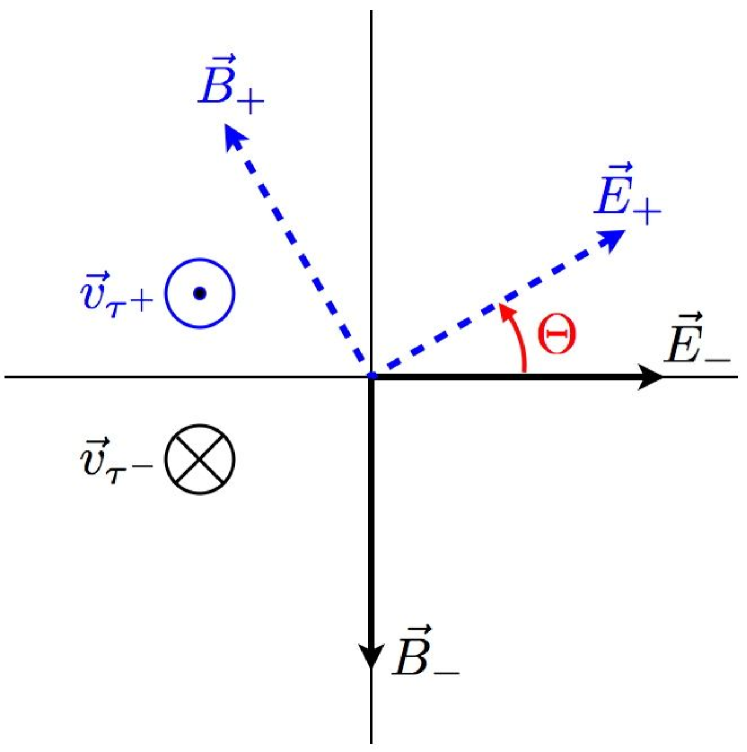
III.3 The angle
We are ready to evaluate in the Higgs rest frame. In this frame, since and are back to back, the – plane and the – plane are parallel to each other. Thus, we will superimpose them to make a single plane. In this combined plane, let and point to the right and downward, respectively. (See figure 1.) Then, we define to be the angle of with respect to , where if is on the upper-half plane, while if on the lower-half plane.555In other words, is the acoplanarity angle between the – plane and – plane, where the orientation of the planes defined by the respective . That is,
| (36) |
where takes values between and . Then makes an angle with respect to . The magnitudes of are the same as the respective . Putting everything together, the distribution (30) becomes
| (37) |
where are given by (35). The contributions that have been neglected to arrive at (37) from (26) are only %.
IV Collider Studies
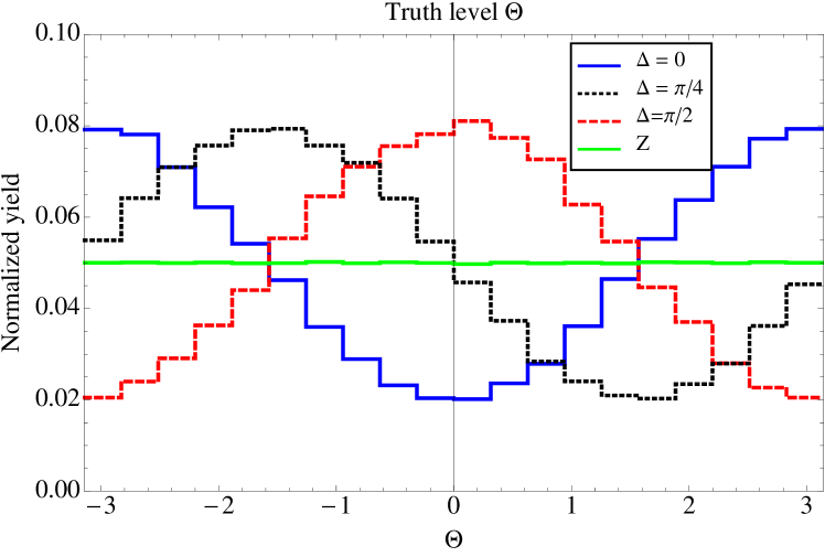
In this section we develop collider analyses aimed at reconstructing the angle in (36). From (23) and (37), the matrix element squared for the decay has a term proportional to : the distribution is thus sensitive to the phase as its minimum is located at . As before, we fix and therefore the only new parameter we introduce is .
We implement the phase in (2) and the effective vertices in (11) and (13) into a FeynRules v.1.6.0 Christensen:2008py model. We then generate Monte Carlo events in MadGraph 5 Alwall:2011uj for production at the LHC with TeV as well as production at the ILC with GeV: in either case, the Higgs decays via . In order to retain quantum interference effects, the full body process is simulated. For the LHC study, we also generate a background sample of production with the subsequent decay .
We will first study the effectiveness of the distribution at truth level, assuming the neutrino momenta are known: this facilitates a comparison to the variable Bower:2002zx ; Worek:2003zp , which was previously proposed for studying violation in the Higgs coupling to taus. After demonstrating the superior qualities of the variable, we present a sensitivity study for reconstructing at the ILC, where the neutrino four-momentum can be reconstructed up to a two-fold ambiguity. Finally, we turn to the LHC, where the neutrinos cannot be reconstructed and the irreducible background is significant. In this case, we find that using a collinear approximation Ellis:1987xu for the neutrino momenta in addition to the standard hard cuts for Higgs events still allows the distribution to retain significant discrimination power between different underlying signal models.
We do not include pileup or perform any detector simulation in this work, aside from implementing flat efficiencies for -tagging for the LHC study. Pileup effects are expected to complicate the primary vertex determination necessary for measuring charged pion tracks as well as contribute extra ambient radiation in the electromagnetic calorimeter (ECAL), making neutral pion momenta measurements more difficult. Furthermore, finite tracking and calorimeter resolutions are expected to smear the distribution. In particular, the ability to distinguish between charged and neutral pion momenta when both pions are overlapping also could affect the measurement. Note, however, that because of the magnetic field, the softer and could be separated at the ECAL. Even if the two pions overlap in the ECAL, the momentum can be obtained by subtracting the track momentum from the total momentum measured in ECAL, assuming negligible contamination from other sources of energy deposition.
We also neglect the neutral pion combinatoric issue, which is justified if the respective parent rho mesons are boosted far apart as a result of the Higgs decay. In general, the and coming from the same parent are mostly collinear. This fact has been exploited in the hadronic tau tagging algorithm. For example, the HPS algorithm used by CMS requires that the charged and neutral hadrons are contained in a cone of the size , where is the transverse momentum of the reconstructed tau Chatrchyan:2012zz . Since the two tau candidates are usually required to be well separated, the combinatorics problem in determining the correct parents can be ignored.
IV.1 Truth level
Recall from (23) and (37) that the minimum of the distribution is located at , and so constructing the distribution allows us to read off the phase of the underlying signal model. In figure 2, we show the distribution in events where we have temporarily assumed the neutrinos are fully reconstructed. The various signal models with (-even), (maximal admixture), and (-odd) clearly show the large contribution of the matrix element as seen in (37). We also superimpose the distribution from event. Note that it is flat. Clearly, observing the cosine oscillation in experimental data will require both a favorable signal to background ratio as well as a solution for the neutrino momenta that preserves the inherently large amplitude of the oscillation.
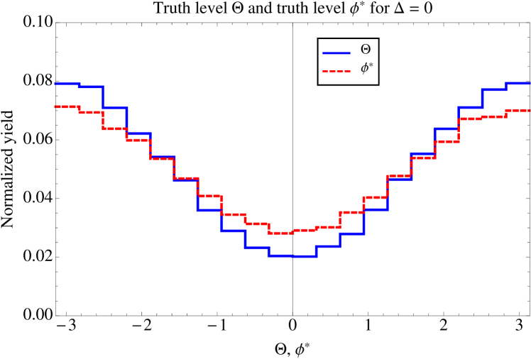
We now compare at truth level with the variable proposed in Refs. Bower:2002zx ; Worek:2003zp : here, is the acoplanarity angle between the decay planes of and in the rest frame. The sign of is defined as the sign of the product of . Following Bower:2002zx ; Worek:2003zp , the events are divided into two classes, and , where the two classes are differ by a phase shift. In order to make a direct comparison with our variable, we combine the distributions of the two classes with a phase shift so the phases of the two classes agree. Note that while does not refer to the neutrinos, this classification into the two classes still requires the knowledge of the neutrino momenta (see (21)). Assuming the neutrinos are fully reconstructed, the and distributions for events are shown in figure 3 with . We readily see that oscillation amplitude of the distribution is larger than that of the acoplanarity angle by about . Compared to , the variable thus provides superior sensitivity to the phase .
Having considered the case where the neutrinos from the tau decays are fully reconstructed, we next turn to the lepton collider environment, where we will find the neutrinos can be fully reconstructed up to a two-fold ambiguity.
IV.2 An Higgs Factory
At a lepton collider running at GeV, such as the ILC, the main production mode for the Higgs is via associated production with a boson. Our prescribed decay mode for the Higgs, , has two neutrinos that escape the detector. We use the known initial four momenta, two tau mass and two neutrino mass constraints to solve for each neutrino momentum component. Note we will assume the decays to visible states, which will reduce our event yield by 20%. Solving the system of equations for the neutrino momenta gives rise to a two-fold ambiguity, where one solution is equal to the truth input neutrino momenta while the other gives a set of wrong neutrino momenta. Note both solutions are consistent with four-momentum conservation and therefore correctly reconstruct the Higgs mass. Since these solutions are indistinguishable in the analysis, we assign each solution half an event weight.
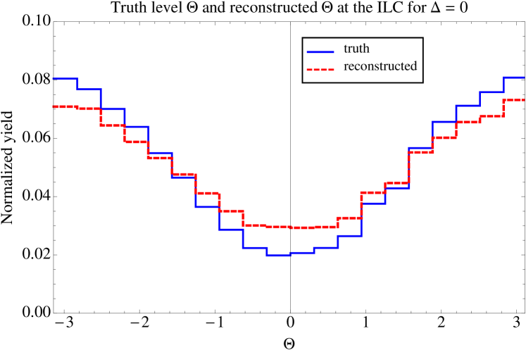
The resulting distribution of for is given in figure 4, where we superimpose the truth level distribution for events for easy comparison. We can see that the oscillation amplitude at the ILC is degraded from the truth level result by . We also show the reconstructed distribution for , , and in figure 5. While the two-fold ambiguity for the neutrino momenta solution set does degrade the truth level result, the reconstructable distribution in figure 5 shows significant discrimination power between various signal models. Note the amplitude of pseudoscalar distribution () is slightly higher than the scalar amplitude: here, the “wrong solution” approximates the correct neutrino momenta on average better than the other or cases. This small effect can be traced back to equation (9) where we derived that a pseudoscalar decays to two taus in the singlet spin state. As a result, in this case the two tau spins point in opposite directions, regardless of the spin quantization axis. In the pseudoscalar case the two tau decays thus tend to occur with opposite orientation and the two neutrinos are slightly more back-to-back and consequently the two solutions for their momenta are closer together.

We now discuss the projected ILC sensitivity for measuring . At the ILC, the cross section for production at GeV with polarized beams for GeV is 0.30 pb ILCTDR .666We have checked the distribution is insensitive to the polarization of the - beams. Assuming a Higgs branching fraction to tau pairs of 6.1%, a branching fraction of 26%, and a -to-visible branching fraction of 80%, we calculate the ILC should have 990 events with 1 ab-1 of luminosity. Since the solved neutrino momenta correctly reconstruct the Higgs mass, the backgrounds are negligible and will be ignored.
| 0.30 pb | |
| Br() | 6.1% |
| Br() | 26% |
| Br( visibles) | 80% |
| N | 990 |
| Accuracy |
To estimate the expected ILC accuracy for measuring , we perform a log likelihood ratio test for the SM hypothesis with against an alternative hypothesis with . In general, the likelihood ratio in bins is given by
| (38) |
where , and are the number of background events, signal events assuming , and signal events assuming in bin of the distribution. In our ILC treatment, we neglect and continuum backgrounds and so we set . Here, is the usual Poisson distribution function, .
We parametrize the signal distribution with a fit function, where the offset constant and oscillation amplitude are fixed by the fit of the standard model distribution with , giving and respectively. Then, the resulting signal distribution is given by . We construct the binned likelihood777We choose bins, though we verified the number of bins is immaterial for our results. according to (38) for various hypotheses to test the discrimination against the SM hypothesis. With 1 ab-1 of ILC luminosity, we find discrimination at , which is a highly promising degree of sensitivity for measuring the phase of the Higgs coupling to taus. We summarize our rate estimate and accuracy result in table 1.
We remark that this sensitivity estimate is only driven by statistical uncertainties, and systematic uncertainties are expected to reduce the efficacy of our result. Also, detector resolution effects and SM backgrounds, while expected to be small, will also slightly degrade our projection. Based on our results, which surpass earlier accuracy estimates of Desch:2003rw , a full experimental sensitivity study incorporating these subleading effects is certainly warranted.
IV.3 LHC
We now develop an LHC study for reconstructing the distribution in in the final state. We use the final state for a couple of reasons. First, since hadronic taus can be faked by jets, two hadronic taus faces an immense background from multijet QCD. By requiring another object in the final state, we gain handles to suppress the background. Second, the collinear approximation gives ambiguous results if the two taus are back-to-back, so the requirement of an additional object in the event guarantees we are away from this configuration. One option is associated production of a Higgs wit a . However this rate is quite small, especially once the branching ratios for into clean final states are taken into account. Other possibilities include Higgs production via vector boson fusion and in association with a jet. Both of these options give promising signal-to-background ratios and both should be considered. For concreteness we will consider here as a demonstration of the feasibility of our technique.
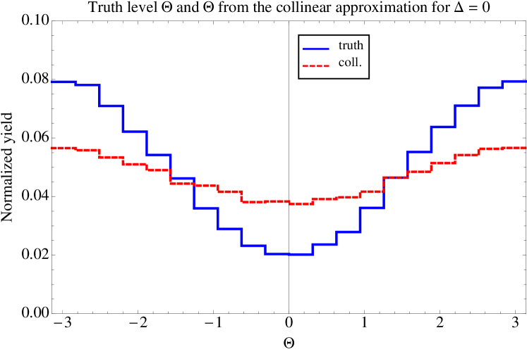
As mentioned before, the neutrinos are not reconstructible in the hadron collider environment, and so we will employ the collinear approximation Ellis:1987xu for the neutrino momenta. In figure 6, we show a comparison between the truth level distribution and the distribution using the collinear approximation for neutrino momenta, for the benchmark. While the collinear approximation reduces the oscillation amplitude of the distribution, the location of the minimum of the distribution does not change. Therefore, measuring is a viable possibility at the LHC using the collinear approximation for the neutrino momenta. We remark that in the collinear approximation, is equivalent to the acoplanarity angle Bower:2002zx ; Worek:2003zp . Yet, we are the first feasibility study for measuring violation in the Higgs coupling to taus at hadron colliders using prompt tau decays and kinematics. With a more sophisticated scheme than the collinear approximation, the variable will be superior to .
At the LHC, the dominant background for the signal process is the irreducible background, where the decays to the same final state as the higgs. As shown earlier in figure 2, the distribution from events is flat: importantly, this is true regardless of possible mass window cuts on the reconstructed resonance. We remark that the phase in the Higgs coupling to taus does manifest in the –– vertex at one loop. Since this effect is suppressed by , whereas the signal to background ratio will be , we can safely ignore the loop induced phase in the –– vertex. In addition, we will assume that the QCD background contribution also has a flat distribution, since the QCD contamination in the signal region is not expected to have any particular spin correlations.
Using our and event samples from MadGraph 5 for a 14 TeV LHC, we first isolate the signal region with a series of hard cuts. First, we apply a preselection requirement on the leading jet GeV with . Using MCFM v.6.6 Campbell:2011bn with these preselection requirements on the leading jet, we obtain a NLO inclusive cross section of 2.0 pb with GeV and a NLO inclusive cross section of 420 pb. After applying the appropriate Higgs, , and tau branching fractions, we calculate a signal cross section of 8.2 fb and background cross section of 970 fb.888These numbers were generated using CTEQ6M parton distribution functions. For the signal we use a factorization/renormalization scale of , while for the background we use . These scale choices are motivated by agreement with higher order (NNLO) calculations (where they exist). Next, we impose hard kinematic cuts to isolate the signal. Motivated by CMS:utj , we choose the signal region to be:
-
•
GeV,
-
•
GeV,
-
•
,
-
•
GeV,
where is the reconstructed Higgs mass by using the collinear approximation. The hard cut strongly suppresses the background, but is less effective on multijet QCD. To reduce the multijet component – and its accompanying uncertainty – to less than 10% of the total background we impose a high cut. The net efficiencies for signal and background after these cuts are 18% and 0.24%, respectively. Rather than simulate the QCD contribution, we account for QCD contamination in the signal region by increasing the background rate by 10%: a complete treatment of the expected QCD background is beyond the scope of this study. Finally, for hadronic tagging efficiency, we consider a standard 50% efficiency and a more optimistic 70% efficiency Chatrchyan:2012zz . We therefore expect 1100 signal events and 1800 QCD background events with 3 ab-1 of luminosity from the 14 TeV LHC, assuming 50% tagging efficiency. These rates are summarized in table 2.
| Inclusive | 2.0 pb | 420 pb |
|---|---|---|
| Br( decay) | 6.1% | 3.4% |
| Br() | 26% | 26% |
| Cut efficiency | 18% | 0.24% |
| N | 1100 | 1800 |
We note that although we generated signal and background samples independently, there is a small interference between Higgs and diagrams in the diagram. Our checks of this interference on the distributions for combined signal and background events versus separate signal and background events showed a negligible effect: we thus ignore this interference effect.
We now perform a likelihood analysis (38) to quantify how effectively the distribution distinguishes between signal hypotheses with different phases in the presence of QCD background. First, we test the discrimination between a pure scalar and a pure pseudoscalar –– coupling. We find that these two hypotheses can be distinguished at sensitivity with 550 (300) fb-1 assuming 50% (70%) tagging efficiency. We can attain sensitivity between pure scalar and pseudoscalar couplings with 1500 (700) fb-1 luminosity assuming 50% (70%) efficiency.
We also estimate the possible accuracy for the LHC experiments to measure with an upgraded luminosity of . We adopt the same procedure as with the ILC accuracy estimate described in the previous section, modified to account for the QCD background, which is fixed to be flat in . We find that the accuracy in measuring is () assuming 50% (70%) hadronic tagging efficiency. The scalar versus pseudoscalar discrimination and the accuracy estimates are summarized in table 3.
| efficiency | 50% | 70% |
|---|---|---|
| Accuracy() |
Again, these estimates are based only on statistical uncertainties without performing a full detector simulation. The effects from pileup and detector resolution are expected to degrade these projections, but corresponding improvements in the analysis, such as a more precise approximation for the neutrino momenta, improved background understanding (from other LHC measurements) or multivariate techniques, could counterbalance the decrease in sensitivity. The promising results of our study strongly motivate a comprehensive analysis by the LHC experiments for the prospect of measuring the phase .
V Conclusions
Higgs decays to tau leptons provide a singular opportunity to measure the properties of the Higgs-fermion couplings. In this paper, we have studied the decay of followed by . A new observable, , was constructed in (36) using the momenta of the tau decay products. The differential cross section can be written in a form of , hence the distribution can be used to distinguish various mixing as shown in figure 2. The variable can be viewed as an acoplanarity angle between the planes spanned by certain linear combinations of the pion and neutrino momenta, and it was demonstrated to be superior to previously proposed acoplanarity angles.
At the ILC, where the neutrino momenta can be reconstructed up to a two-fold ambiguity, the advantages of the variable are most evident. We estimate that the phase can be measured to an accuracy of for GeV, a substantial improvement over previous results. For the LHC, we have had to rely on the collinear approximation to reconstruct the neutrino momenta and some of the discriminating power of the variable is lost. Nevertheless, we find an accuracy of () is possible after 3000 fb-1 of luminosity and assuming a 50% (70%) tau tagging efficiency. Recasting in terms of the parameters introduced in (3), a – deviation from the SM case is equivalent to sensitivity to TeV, where is the scale of the dimension six operator in (3) and is assumed to be . A better approximation scheme for the neutrino momenta will improve these results.
In our collider studies we have neglected detector effects and background systematic uncertainties. While adding these effects will worsen our results, this may be offset by better understanding of the backgrounds (thereby allowing looser cuts) and with a more sophisticated (e.g. MVA) analysis and statistical tools.
Finally, in this work we picked specific Higgs production mechanisms and focused on a single decay channel. To understand the full extent of future colliders’ sensitivities to the phase of Higgs-fermion couplings, additional production channels such as VBF should be explored, both at the LHC and in a Higgs factory. In addition, other hadronic decay channels, as well as semi-leptonic channels, of the tau pair might also be sensitive to the properties of the Higgs.
Acknowledgements.
We would like to thank Kaustubh Agashe, Wolfgang Altmannshofer, Yuval Grossman, Uli Haisch, Josh Ruderman, Daniel Stolarski, Raman Sundrum, Ciaran Williams and Jure Zupan for comments and discussions. We would also like to thank the Kavli Institute for Theoretical Physics at UCSB where part of this work was performed. RP is supported by the NSF under grant PHY-0910467. TO is supported by the DOE under grant DE-FG02-13ER41942. Fermilab is operated by the Fermi Research Alliance, LLC under Contract No. De-AC02-07CH11359 with the United States Department of Energy.Appendix A A Simple UV Completion of the Dimension-6 Operator
In this appendix we give an example for a UV completion for the dimension-6 operator in (3), i.e., the term with . Our purpose is not to advocate a specific model as particularly well-motivated but to simply provide an existence proof of a weakly-coupled renormalizable theory that can generate the term in (3) at with an arbitrary phase, without generating other operators that may contradict with experiments.
Consider an extension of the SM with a second higgs doublet with with the following tree-level lagrangian:
| (39) | ||||
where is the SM lagrangian without the tau Yukawa coupling. The full quantum lagrangian is , where contains all counterterms necessary for consistent renormalization at loop level. For simplicity, we neglect neutrino masses and mixings, so possesses an accidental family symmetry, which is then inherited by as well. This immediately implies that there are no lepton flavor changing processes such as . There are no constraints from quark flavor/ measurements; since the couplings of to quarks are absent in and only appear in , they are not only very small ( the corresponding SM Yukawa) but also respect the CKM flavor structure of the SM. Similarly, the couplings of to and are inconsequential; in particular, we have checked that a contribution to the electron elecric dipole moment induced at 2-loop level is negligible. Finally, the modification of the coupling of to is also tiny, safely below the LEP constraints.
In order to see the effects of (39) on Higgs decays let us consider the limit in which and the doublet can be integrated out and we can consider an effective field theory below . At tree level, this generates two dimension-6 interactions:
| (40) |
This theory now matches on to the effective theory (3) with , and . It should be noted that this theory contains in general a violating phase. In particular, the phase of may not be rotated away by field redefinitions. Taking and with arbitrary phases in , and can therefore produce an -violating phase in Higgs decays to tau leptons.
Other theories, including composite Higgs models Agashe:2004rs ; Giudice:2007fh and models with vector-like leptons Kearney:2012zi may also produce the necessary interactions to induce violating Higgs decays into taus. In constructing such models one should take care that the coupling of to taus is not modified above the level (see Ref. ALEPH:2005ab or Fig. 10.4 of Beringer:1900zz ) either by construction (as in the model we just discussed) or by a cancellation among various contributions.
References
- (1) G. Aad et al. [ATLAS Collaboration], Phys. Lett. B 716, 1 (2012) [arXiv:1207.7214 [hep-ex]].
- (2) S. Chatrchyan et al. [CMS Collaboration], Phys. Lett. B 716, 30 (2012) [arXiv:1207.7235 [hep-ex]].
- (3) [ATLAS Collaboration], ATLAS-CONF-2013-034. [CMS Collaboration], CMS-PAS-HIG-13-005.
- (4) T. Aaltonen et al. [CDF and D0 Collaborations], arXiv:1303.6346 [hep-ex].
- (5) S. Chatrchyan et al. [CMS Collaboration], Phys. Rev. Lett. 110, 081803 (2013) [arXiv:1212.6639 [hep-ex]].
- (6) [ATLAS Collaboration], ATLAS-CONF-2013-013.
- (7) S. Bolognesi, Y. Gao, A. V. Gritsan, K. Melnikov, M. Schulze, N. V. Tran and A. Whitbeck, Phys. Rev. D 86, 095031 (2012) [arXiv:1208.4018 [hep-ph]].
- (8) Y. Grossman and I. Nachshon, JHEP 0807, 016 (2008) [arXiv:0803.1787 [hep-ph]].
- (9) F. Bishara, Y. Grossman, R. Harnik, D. Robinson, J. Shu and J. Zupan, in progress.
- (10) R. Primulando, D. Stolarski and J. Zupan, in progress.
- (11) [CMS Collaboration], CMS-PAS-HIG-13-004.
- (12) J. R. Dell’Aquila and C. A. Nelson, Nucl. Phys. B 320, 86 (1989).
- (13) J. R. Dell’Aquila and C. A. Nelson, Nucl. Phys. B 320 (1989) 61.
- (14) B. Grzadkowski and J. F. Gunion, Phys. Lett. B 350, 218 (1995) [hep-ph/9501339].
- (15) G. R. Bower, T. Pierzchala, Z. Was and M. Worek, Phys. Lett. B 543, 227 (2002) [hep-ph/0204292].
- (16) M. Worek, Acta Phys. Polon. B 34, 4549 (2003) [hep-ph/0305082].
- (17) K. Desch, Z. Was and M. Worek, Eur. Phys. J. C 29, 491 (2003) [hep-ph/0302046].
- (18) K. Desch, A. Imhof, Z. Was and M. Worek, Phys. Lett. B 579, 157 (2004) [hep-ph/0307331].
- (19) S. Berge and W. Bernreuther, Phys. Lett. B 671, 470 (2009) [arXiv:0812.1910 [hep-ph]].
- (20) S. Berge, W. Bernreuther and J. Ziethe, Phys. Rev. Lett. 100, 171605 (2008) [arXiv:0801.2297 [hep-ph]].
- (21) S. Berge, W. Bernreuther, B. Niepelt and H. Spiesberger, Phys. Rev. D 84, 116003 (2011) [arXiv:1108.0670 [hep-ph]].
- (22) S. Berge, W. Bernreuther and H. Spiesberger, arXiv:1208.1507 [hep-ph].
- (23) R. K. Ellis, I. Hinchliffe, M. Soldate and J. J. van der Bij, Nucl. Phys. B 297, 221 (1988).
- (24) N. D. Christensen and C. Duhr, Comput. Phys. Commun. 180, 1614 (2009) [arXiv:0806.4194 [hep-ph]].
- (25) J. Alwall, M. Herquet, F. Maltoni, O. Mattelaer and T. Stelzer, JHEP 1106 (2011) 128 [arXiv:1106.0522 [hep-ph]].
- (26) C. Collaboration et al. [CMS Collaboration], JINST 7, P01001 (2012) [arXiv:1109.6034 [physics.ins-det]].
- (27) ILC Technical Design Report, Vol. 2, [ILC Collaboration] http://www.linearcollider.org/ILC/TDR
- (28) J. M. Campbell, R. K. Ellis and C. Williams, JHEP 1107, 018 (2011) [arXiv:1105.0020 [hep-ph]].
- (29) K. Agashe, R. Contino and A. Pomarol, Nucl. Phys. B 719, 165 (2005) [hep-ph/0412089].
- (30) G. F. Giudice, C. Grojean, A. Pomarol and R. Rattazzi, JHEP 0706 (2007) 045 [hep-ph/0703164].
- (31) J. Kearney, A. Pierce and N. Weiner, Phys. Rev. D 86, 113005 (2012) [arXiv:1207.7062 [hep-ph]].
- (32) S. Schael et al. [ALEPH and DELPHI and L3 and OPAL and SLD and LEP Electroweak Working Group and SLD Electroweak Group and SLD Heavy Flavour Group Collaborations], Phys. Rept. 427, 257 (2006) [hep-ex/0509008].
- (33) J. Beringer et al. [Particle Data Group Collaboration], Phys. Rev. D 86, 010001 (2012).