BIPOLAR MAGNETIC STRUCTURES DRIVEN BY STRATIFIED TURBULENCE WITH A CORONAL ENVELOPE

Abstract

We report the spontaneous formation of bipolar magnetic structures in direct numerical simulations of stratified forced turbulence with an outer coronal envelope. The turbulence is forced with transverse random waves only in the lower (turbulent) part of the domain. Our initial magnetic field is either uniform in the entire domain or confined to the turbulent layer. After about 1–2 turbulent diffusion times, a bipolar magnetic region of vertical field develops with two coherent circular structures that live during one turbulent diffusion time, and then decay during 0.5 turbulent diffusion times. The resulting magnetic field strengths inside the bipolar region are comparable to the equipartition value with respect to the turbulent kinetic energy. The bipolar magnetic region forms a loop-like structure in the upper coronal layer. We associate the magnetic structure formation with the negative effective magnetic pressure instability in the two-layer model.

1. Introduction

Sunspots are visible surface manifestations of magnetic fields inside the Sun. The magnetic fields in sunspots are sufficiently strong to suppress the transport of heat via convective motions and therefore they appear as dark on the solar disk. We are now able to study them with high-resolution telescopes (Scharmer et al., 2011) as well as with realistic numerical simulations (Rempel et al., 2009) to discover new properties of sunspots. However, their formation mechanism is still a subject of active discussion.

It is broadly believed that sunspots are caused by emerging flux tubes (Parker, 1955) that are generated at the bottom of the convection zone (Parker, 1975). The magnetic flux tubes become unstable and rise until they pierce the solar surface to form bipolar regions and pairs of sunspots (Caligari et al., 1995). The rise of flux tubes and the decay of the resulting active regions is also an ingredient in some dynamo theories to explain the 22 yr cyclic behavior of the solar magnetic field (e.g., Nandy & Choudhuri, 2001; Choudhuri, 2003). However, these theories assume the existence of thin, isolated magnetic flux tubes at the bottom of the convection zone with fields of the order of $10^{5}\,{\rm G}$. In direct numerical simulations (DNS) of solar dynamos, thin flux tubes of comparable strength have not yet been found (e.g., Guerrero & Käpylä, 2011; Nelson et al., 2013; Käpylä et al., 2013). There is no conclusive evidence of rising magnetic flux tubes from helioseismology either; see Birch et al. (2010, 2013), who also comment on a detection reported by Ilonidis et al. (2011). These difficulties have led to an alternative approach in which sunspots are formed as shallow phenomena near the solar surface (Brandenburg, 2005).

The formation of bipolar regions has recently been found in realistic radiation-magnetohydrodynamics (MHD) simulations of near-surface convection (Stein & Nordlund, 2012), were kG magnetic fields were inserted at the bottom of a $20$ Mm deep box. The authors argue that deep downdrafts associated with the supergranulation concentrate the magnetic field and determine thereby the scale of their separation. They also emphasize the importance of radiative cooling at the surface.

Two alternative mechanisms for the spontaneous formation of flux concentrations have been discussed in the literature. One is based on a turbulent thermo-magnetic instability in small-scale turbulence with radiative boundaries, where the magnetic quenching of the turbulent convective heat transport is used in mean-field simulations (MFSs) to produce flux concentrations (Kitchatinov & Mazur, 2000). The other mechanism is based on the suppression of the total turbulent pressure (the sum of hydrodynamic and magnetic contributions) by the magnetic field. This leads to the so-called negative effective magnetic pressure instability (NEMPI), which is another mechanism that forms flux concentrations in a stratified turbulent medium (see, e.g., Brandenburg et al., 2011; Kemel et al., 2012). The original idea of NEMPI goes back to early work by Kleeorin et al. (1989, 1990) and has led to numerous studies both analytically (Kleeorin & Rogachevskii, 1994; Kleeorin et al., 1996; Rogachevskii & Kleeorin, 2007) and through DNS and MFS (Brandenburg et al., 2010, 2012; Losada et al., 2012, 2013a, 2013b; Jabbari et al., 2013).

More recently, Brandenburg et al. (2013b) found super-equipartition magnetic field concentrations in DNS by imposing a relatively weak vertical magnetic field on forced strongly stratified turbulence. Their results may be related to earlier simulations of turbulent convection in which a vertical magnetic field was found to segregate into magnetized and unmagnetized regions (Tao et al., 1998), but it is still unclear whether those results are also caused by NEMPI or by some other mechanism that still remains to be understood. However, neither the turbulent thermo-magnetic instability nor NEMPI have yet been able to produce bipolar magnetic regions. Except for the work of Stein & Nordlund (2012), bipolar regions have previously been studied by advecting a semi-torus shaped twisted flux tube of 9 kG through the bottom boundary at a 7.5 Mm depth of thermally relaxed convection (Cheung et al., 2010).

In the current study we demonstrate that bipolar regions can be obtained naturally in DNS in the presence of an outer coronal layer. Indeed, all previous simulations of NEMPI and the turbulent thermo-magnetic instability have a rigid upper boundary, which is clearly unrealistic. In this Letter we alleviate the constraints from a rigid upper boundary by combining NEMPI in a forced turbulent layer with a coronal envelope at the top. This approach has been successful in generating plasmoids reminiscent of coronal mass ejections (Warnecke et al., 2011). In that work, a simplified corona is combined with a large-scale dynamo that is either generated by forced turbulence in a Cartesian domain (Warnecke & Brandenburg, 2010) or in spherical coordinates (Warnecke et al., 2011), or through self-consistent turbulent convection (Warnecke et al., 2012b). This approach leads to a more realistic “boundary condition” at the interface between the dynamo and corona without using, for example, radiative transfer. Not only has it led to coronal ejections, but also to the discovery of a change of sign of magnetic helicity some distance away from the star (Warnecke et al., 2012a), and the realization that both the dynamo and the differential rotation may be affected by the presence of a free boundary as modeled by the coronal envelope (Warnecke et al., 2013).

For a more realistic model, several other factors need to be accounted for. Except for radiation and ionization that would potentially lead to new effects (see, e.g., Barekat & Brandenburg, 2013), which might distort our interpretation, there would be the issue of the origin of the magnetic field itself. It should really come from a self-consistent large-scale dynamo beneath the surface. Again, this leads to new complications, through its interaction with NEMPI, which have only recently been addressed by Jabbari et al. (2013) and Losada et al. (2013a). To avoid of those complications, we take a horizontal magnetic field as the initial condition. We mainly consider the case of a uniform magnetic field that is then also present in the corona at all times (case A), and compare with a case in which it is initially only in the turbulence layer, but slowly decaying (case B). These fields are weak, but they might have interesting unexpected and unexplored effects that will be the topic of the current Letter. At this point we cannot be certain that it has direct applications to the Sun, but in view of the fact that research into NEMPI has been growing rapidly, it is important to explore all aspects of it before we can make definitive statements about its applicability to sunspots.

2. The model

Our model is similar to that of Brandenburg et al. (2013b), where they solve the isothermal hydromagnetic equations in the presence of vertical gravity $\mbox{\boldmath$g$}{}=(0,0,-g)$, but here the random nonhelical forcing $f$ acts just in the lower part ($-\pi<z<0$) of a Cartesian domain of size $L_{x}\times L_{y}\times L_{z}$, where $L_{x}=L_{y}=2\pi$ and $L_{z}=3\pi$. Also, instead of a vertical field, we now take a weak uniform horizontal magnetic field, either as an imposed one throughout the domain, $\mbox{\boldmath$B$}{}_{\rm imp}=(0,B_{0},0)$ with $\mbox{\boldmath$A$}{}={\bf 0}$ (case A), or as an initial one in the lower part ($z<0$) by putting $A_{x}=-\max(0,-z)\,B_{0}$ and $\mbox{\boldmath$B$}{}_{\rm imp}={\bf 0}$ (case B). Similar to Warnecke & Brandenburg (2010), we employ a forcing function $\mbox{\boldmath$f$}{}(\bm{x},t)$ that is modulated by

$$\theta_{w}(z)={\textstyle{1\over 2}}\left(1-{\rm erf}{z\over w}\right),$$ (1)

where $w$ is the width of the transition. We thus solve the equations for the velocity $u$, the magnetic vector potential $A$, and the density $\rho$:

$${D\mbox{\boldmath$u$}{}\over Dt}=\mbox{\boldmath$g$}{}+\theta_{w}(z)\mbox{\boldmath$f$}{}+{1\over\rho}[-c_{\rm s}^{2}\mbox{\boldmath$\nabla$}{}\rho+\mbox{\boldmath$J$}{}\times\mbox{\boldmath$B$}{}+\mbox{\boldmath$\nabla$}{}\cdot(2\nu\rho\mbox{\boldmath${\sf S}$}{})],$$ (2)

$${\partial\mbox{\boldmath$A$}{}\over\partial t}=\mbox{\boldmath$u$}{}\times\mbox{\boldmath$B$}{}+\eta\nabla^{2}\mbox{\boldmath$A$}{},$$ (3)

$${D\ln\rho\over Dt}=-\mbox{\boldmath$\nabla$}{}\cdot\mbox{\boldmath$u$}{},$$ (4)

where $\nu$ is the kinematic viscosity, $\eta$ is the magnetic diffusivity, $\mbox{\boldmath$B$}{}=\mbox{\boldmath$B$}{}_{\rm imp}+\mbox{\boldmath$\nabla$}{}\times\mbox{\boldmath$A$}{}$ is the magnetic field, $\mbox{\boldmath$J$}{}=\mbox{\boldmath$\nabla$}{}\times\mbox{\boldmath$B$}{}/\mu_{0}$ is the current density, $\mu_{0}$ is the vacuum permeability, ${\sf S}_{ij}={\textstyle{1\over 2}}(u_{i,j}+u_{j,i})-{\textstyle{1\over 3}}\delta_{ij}\mbox{\boldmath$\nabla$}{}\cdot\mbox{\boldmath$u$}{}$ is the traceless rate of strain tensor, and commas denote partial differentiation. The forcing function $f$ consists of random, white-in-time, plane non-polarized waves (Haugen & Brandenburg, 2004) with an average wavenumber $k_{\it f}=30\,k_{1}$, where $k_{1}=2\pi/L_{x}$ is the lowest wavenumber in the domain in the horizontal direction. The forcing strength is such that the turbulent rms velocity is approximately independent of $z$ with $u_{\rm rms}=\langle\mbox{\boldmath$u$}{}^{2}\rangle^{1/2}\approx 0.1\,c_{\rm s}$. The value of the gravitational acceleration $g$ is related to the density scale height $H_{\rho}=c_{\rm s}^{2}/g$ and is chosen such that $k_{1}H_{\rho}=1$, which leads to a density contrast between bottom and top of $\exp(3\pi)\approx 1.2\times 10^{4}$.

Except for the profile of the forcing function and the extent of the domain, our setup is also similar to Kemel et al. (2012), who used the same values of the fluid Reynolds number $\mbox{\rm Re}\equiv u_{\rm rms}/\nu k_{\it f}=38$, the magnetic Prandtl number $\mbox{\rm Pr}_{M}\equiv\nu/\eta=1/2$, and thus of the magnetic Reynolds number $\mbox{\rm Re}_{M}\equiv\mbox{\rm Re}\,\mbox{\rm Pr}_{M}=19$, which is known to lead to negative effective magnetic pressure for the mean magnetic fields, $\overline{\mbox{\boldmath$B$}}{}$, in the range $0<|\overline{\mbox{\boldmath$B$}}{}|/B_{\rm eq}<0.4$. Here, $\overline{\mbox{\boldmath$B$}}{}$ is obtained by averaging over the scale of several turbulent eddies. The magnetic field is expressed in units of the local equipartition field strength, $B_{\rm eq}=\sqrt{\mu_{0}\rho}\,u_{\rm rms}$, while the initial magnetic field $B_{0}$ is specified in units of the value at $z=0$, namely $B_{\rm eq0}=\sqrt{\mu_{0}\rho_{0}}\,u_{\rm rms}$, where $\rho_{0}=\rho(z=0)$. We use $B_{0}/B_{\rm eq0}=0.02$, which is also the field strength used in the main run of Brandenburg et al. (2013b). Time is expressed in turbulent-diffusive times, $\tau_{\rm td}=(\eta_{\rm t0}k_{1}^{2})^{-1}$, where $\eta_{\rm t0}=u_{\rm rms}/3k_{\it f}$ is the estimated turbulent magnetic diffusivity.

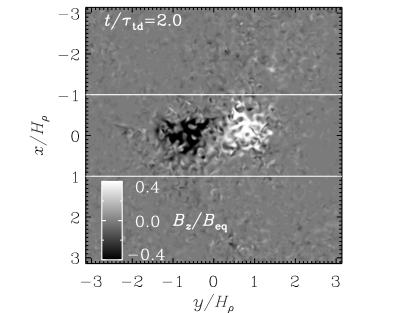
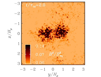
Figure 1.— Left panel: normalized vertical magnetic field $B_{z}/B_{\rm eq}$ of the bipolar region at the surface ($z=0$) of the simulation domain. The white lines delineate the area shown in Figure 3. Right panel: normalized magnetic energy $\mbox{\boldmath$B$}{}^{2}/B_{\rm eq}^{2}$ of the two regions relative to the rest of the surface. Note that we clip both color tables to increase the contrast of the structure. The field strength reaches around $B_{z}/B_{\rm eq}=1.4$. Case A.

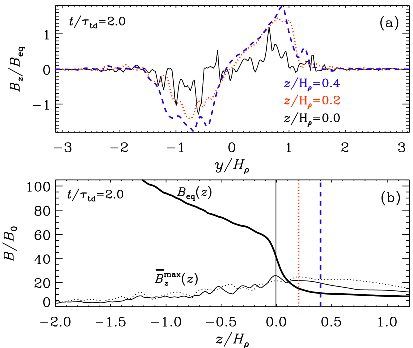
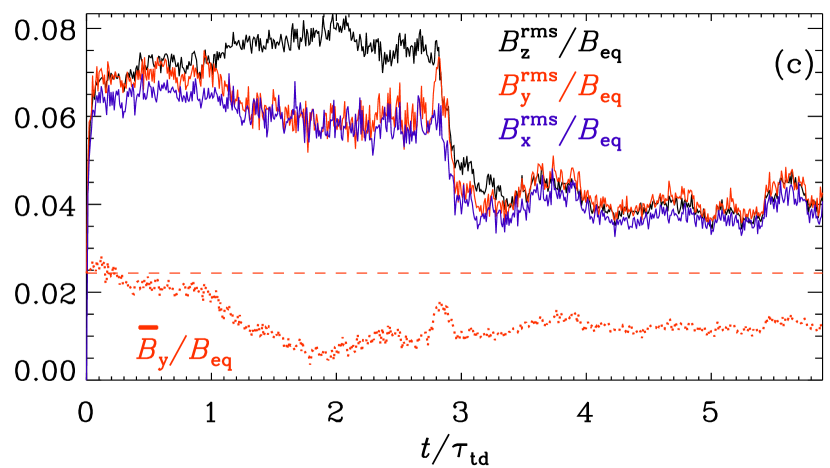
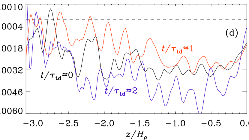
Figure 2.— (a) Profiles of $B_{z}(y)/B_{\rm eq}$ through $x=0$ at three heights ($z/H_{\rho}=0,0.2,0.4$), whose values are indicated also by vertical bars in the next panel. (b) Vertical profiles of $B_{\rm eq}(z)/B_{0}$ (thick solid line) and $\overline{B}_{z}^{\max}(z)/B_{0}$, shown as a regular solid line at $t/\tau_{\rm td}=2.0$. The dotted lines show the profiles of $\overline{B}_{z}^{\max}(z)/B_{0}$, which are similar to those of $-\overline{B}_{z}^{\min}(z)/B_{0}$. (c) Growth and decay of the different magnetic field components at the surface ($z$=0). The solid lines represent the rms of the vertical field $B_{z}^{\rm rms}=\langle B_{z}^{2}\rangle_{xy}$ (black), and the horizontal $B_{y}^{\rm rms}=\langle B_{y}^{2}\rangle_{xy}$ (red), $B_{x}^{\rm rms}=\langle B_{x}^{2}\rangle_{xy}$ (blue). The horizontal averaged magnetic field in the direction of the initial field $\overline{B}_{y}=\langle B_{y}\rangle_{xy}$ is shown with a dotted red line, the value of the initial field is indicated by a dashed red line. All values are normalized by the equipartition field strength at the surface. (d) Effective magnetic pressure ${\cal P}_{\rm eff}$ over height $z$. The three lines indicate different times during the simulation: $t/\tau_{\rm td}\approx 0$ (black), $t/\tau_{\rm td}\approx 1$ (red) and $t/\tau_{\rm td}\approx 2$ (blue). The pressure is averaged over a time interval $\Delta t/\tau_{\rm td}\approx 0.15$ and smoothed over four grid points. The dashed line represents the zero line. Case A.

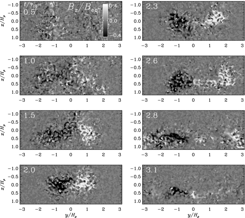
Figure 3.— Visualizations of horizontal cross-sections of $B_{z}(x,y)/B_{\rm eq}$ through $z=0$, for case A, similar to Figure 1, but only data in $-1.2\leq x/H_{\rho}\leq 1.2$ are shown.

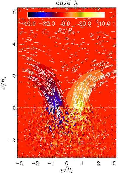
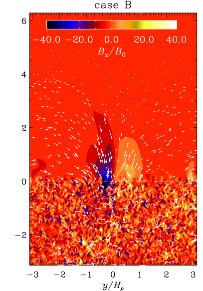
Figure 4.— Visualizations of vertical cross-sections of $B_{z}(y,z)/B_{0}$ together with magnetic field vectors in the $yz$ plane through the $x$ location of the flux convergence for case A at $t/\tau_{\rm td}=2.0$ (left) and case B at $t/\tau_{\rm td}=1.83$ (right). The dash-dotted lines indicate the surface at $z=0$.

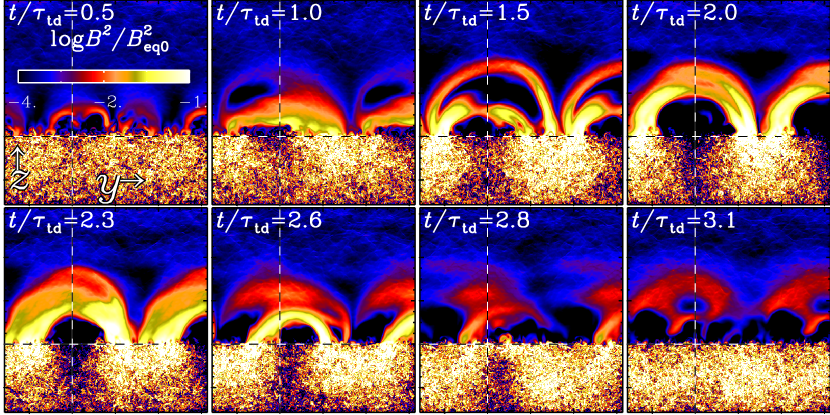
Figure 5.— Time series of normalized magnetic energy density $\mbox{\boldmath$B$}{}^{2}/B_{\rm eq0}^{2}$ in a vertical cut through the bipolar region at $x=0$ for case A. The domain has been replicated by 50% in the $y$ direction to give a more complete impression about spot separation and arch length. The black-white dashed lines mark the surface ($z=0$) and the replicated part.

The simulations are performed with the Pencil Code, which uses sixth-order explicit finite differences in space and a third-order accurate time stepping method. We use a resolution of $256\times 256\times 512$ mesh points in the $x$, $y$, and $z$ directions. We adopt periodic boundary conditions in the $xy$ plane and present our results by shifting our coordinate system such that the regions of interest lie at the center around $x=y=0$. On $z=-\pi$ we apply a stress-free perfect conductor condition and on $z=2\pi$ a stress-free vertical field condition.

3. Results

We report the spontaneous formation and decay of bipolar magnetic regions at the surface ($z=0$), which is the boundary between regions with and without forcing. These two parts resemble the upper convection zone and a simplified corona of the Sun. In Figure 1, we show for case A the bipolar region as the normalized vertical magnetic field $B_{z}/B_{\rm eq}$ (left panel) and the normalized magnetic energy $\mbox{\boldmath$B$}{}^{2}/B_{\rm eq}^{2}$ (right panel) at the moment of maximum strength, $t/\tau_{\rm td}=2$. Note that the $y$ direction points to the right, while the positive $x$ direction points downward, so the coordinate system has been rotated by $90^{\circ}$ to allow a view that is more similar to how bipolar regions are oriented on the solar disk. The shapes of both magnetic spots are nearly circular, but are still disturbed by the turbulent motion acting on the magnetic field. The field outside this bipolar region is weak: almost all the magnetic field is concentrated inside the bipolar region. At and slightly above $z=0$, we find field strengths significantly above the equipartition value. This is seen more clearly in Figure 2(a), where we show for case A profiles of $B_{z}(y)/B_{\rm eq}$ through $x=0$ at three heights. We normalize the magnetic field by its local equipartition value, $B_{\rm eq}(z)$ (Figure 2a) or by the strength of the initial field $B_{0}$ (Figure 2b). The field $B_{\rm eq}(z)$ is also shown as a thick line in Figure 2(b). At the surface we have $B_{\rm eq}(0)/B_{0}\approx 50$, but for $z>0$ it drops sharply to values below 20. At each height, we have computed maximum and minimum field strengths of the mean field, $\overline{\mbox{\boldmath$B$}}{}$, defined here by Fourier filtering to include only wavenumbers below $k_{\it f}/2$, as functions of $z$, i.e., $\overline{B}_{z}^{\max}(z)$ and $-\overline{B}_{z}^{\min}(z)$, respectively. It turns out that $\overline{B}_{z}^{\min}(z)\approx-\overline{B}_{z}^{\max}(z)$, and that both decline more slowly with height than $B_{\rm eq}$, so the field reaches super-equipartition strength in the outer parts.

We recall that in case A, we have $\mbox{\boldmath$B$}{}_{0}=\mbox{\boldmath$B$}{}_{\rm imp}$ over the whole domain. However, the field quickly becomes tangled by the random velocity field in $z<0$ where the forcing is acting to produce small-scale magnetic fields on the scale of the turbulence. In the upper part, however, this horizontal field stays roughly unchanged up to the instant when it becomes affected by a large-scale instability (NEMPI). As shown in Figure 2(c), the rms values of the three components of the magnetic field at the surface ($z=0$) grow rapidly until they saturate at $t/\tau_{\rm td}\approx 0.2$. At $t/\tau_{\rm td}\approx 1$, the magnetic field has attained a strong vertical component while the horizontal one declines. By the time $t/\tau_{\rm td}=2$, the vertical field is stronger than the horizontal field until all three components decay rapidly to a lower value and saturate there.

To see whether the increase of vertical magnetic field and structure formation is related to NEMPI, we show in Figure 2(d) that the effective magnetic pressure ${\cal P}_{\rm eff}$ is indeed negative below the surface in the turbulent region for case A. It can be calculated using an approach applied by Brandenburg et al. (2012):

$${\cal P}_{\rm eff}={\overline{\mbox{\boldmath$B$}}{}^{2}\over 2B_{\rm eq}^{2}}+{\left(\Pi_{xx}^{(B)}-\Pi_{xx}^{(0)}+\Pi_{zz}^{(B)}-\Pi_{zz}^{(0)}\right)\over B_{\rm eq}^{2}},$$ (5)

where $\Pi_{ij}^{(B)}\equiv\overline{\rho u_{i}u_{j}}+{\textstyle{1\over 2}}\delta_{ij}\mu_{0}^{-1}\overline{\mbox{\boldmath$b$}{}^{2}}-\mu_{0}^{-1}\overline{b_{i}b_{j}}$ and $\Pi_{ij}^{(0)}$ are the components of the total (Reynolds and Maxwell) turbulent stress tensor with and without mean magnetic influence, respectively, and $\delta_{ij}$ is the unit Kronecker tensor.

Horizontal cross-sections of $B_{z}(x,y)/B_{\rm eq}$ through $z=0$ are shown in Figure 3 for case A at different times. At $t/\tau_{\rm td}=1$, structures begin to form that become more coherent and more circular while decreasing their distance to a minimum until they lie directly next to each other ($t/\tau_{\rm td}=2$). This is also the time of maximum field strength and maximum coherence, and agrees with the peak of $B_{z}^{\rm rms}$ in Figure 2(c). After this time, the distance and field strength of the two polarities decrease until no large-scale structures are visible ($t/\tau_{\rm td}=3.5$).

In Figure 4 we compare $yz$ slices through the bipolar region for cases A and B. The vertical magnetic field is color coded and arrows indicate magnetic field vectors in the plane. The field in the region of $z>3$ is not strongly disturbed by the structure formation and represents $B_{\rm imp}$ in case A and is $\approx 0$ in case B. The weaker field concentration in case B might be related to the decay of the initial field. In both cases, the bipolar spot orientation is peculiar because an emerging flux tube with similar field direction as the imposed field would cause an inverted vertical flux configuration.

The formation of magnetic structures can be caused by the negative contribution of turbulence to the effective large-scale magnetic pressure (the sum of turbulent and non-turbulent contributions). For large magnetic Reynolds numbers, the turbulent contributions are larger than the non-turbulent ones, and the effective magnetic pressure becomes negative; see Figure 2(d). This results in a large-scale instability, which causes a redistribution of mass so that a large-scale flow is generated. This flow may also drive the magnetic field patches together. Since turbulence has produced similar strengths for all three components of the magnetic field, and since NEMPI allows for stronger vertical fields than horizontal ones (Brandenburg et al., 2013b), the result is the formation of strong vertical field structures.

It is important to realize that our setup corresponds to an initial value problem in the sense that the magnetic field affects the effective magnetic pressure. It changes the horizontally symmetric background state, which is unstable with respect to NEMPI. This leads to the formation of magnetic structures that tend to stabilize the system. This is the reason why, with our present setup, a bipolar magnetic region occurs only once. Of course, if we apply this mechanism to the Sun, the imposed magnetic field would be provided by a dynamo acting in the convection zone, which would certainly show cycles and fluctuations.

In the coronal region, magnetic loops form that connect the far ends of spots of opposite polarity, as can be seen by plotting 1.5 times the full periodic length in the $y$ direction. In Figure 5 we show for case A the temporal evolution of the normalized magnetic energy density $\mbox{\boldmath$B$}{}^{2}/B_{\rm eq}^{2}$ in such a $yz$ slice. The large-scale loop is strongest at $t/\tau_{\rm td}\approx 2$ when the two magnetic spots are most concentrated. An exploratory run with a larger extent in the $y$-direction resulted in similarly oriented bipolar structures with somewhat larger separation.

4. Conclusions

The current study has shown for the first time that a bipolar magnetic region can emerge and later decay as a natural consequence of stratified turbulence with a coronal envelope and a sufficiently large domain size. For the formation process of the bipolar region, radiative cooling and a particular large-scale flow topology as in Stein & Nordlund (2012) seem to be unimportant. However, they will certainly play a role in determining the detailed structure of sunspots (Rempel et al., 2009; Cheung et al., 2010). The interaction with a weak pre-existing coronal field is not unrealistic. A similar interaction has previously been employed in connection with the production of X-ray jets and flares (Isobe et al., 2005). It supports the formation of a bipolar region (case A), but is otherwise not critical (case B). On the other hand, preliminary calculations with a potential field boundary condition and no corona have not yet resulted in bipolar regions.

We find the two polarities approaching each other in the forming process and separating in the decaying phase. This is an important aspect that was not previously expected from turbulent processes (Spruit, 2012). The observed formation of the bipolar regions in cases A and B is consistent with NEMPI, which predicts that, even though the optimal field strength for the excitation of NEMPI is significantly below the equipartition value, the magnetic field strengths inside the bipolar region can be significantly above the equipartition value of the turbulence at and slightly above the surface (Brandenburg et al., 2013a).

Useful extensions of the model include more realistic stratifications such as a polytropic one in the lower turbulent part (Losada et al., 2013b) combined with a sharp drop in temperature in the upper layer caused by ionization and radiation. Furthermore, above the chromosphere the temperature should increase again in the solar corona (cf. Warnecke et al., 2013).

References

- Barekat & Brandenburg (2013) Barekat, A., & Brandenburg, A. 2013, A&A, submitted (arXiv:1308.1660)
- Birch et al. (2010) Birch, A. C., Braun, D. C., & Fan, Y. 2010, ApJ, 723, L190
- Birch et al. (2013) Birch, A. C., Braun, D. C., Leka, K. D., Barnes, G., & Javornik, B. 2013, ApJ, 762, 131
- Brandenburg (2005) Brandenburg, A. 2005, ApJ, 625, 539
- Brandenburg et al. (2013a) Brandenburg, A., Gressel, O., Jabbari, S., Kleeorin, N., & Rogachevskii, I. 2013a, A&A, submitted (arXiv:1309.3547)
- Brandenburg et al. (2011) Brandenburg, A., Kemel, K., Kleeorin, N., Mitra, D., & Rogachevskii, I. 2011, ApJ, 740, L50
- Brandenburg et al. (2012) Brandenburg, A., Kemel, K., Kleeorin, N., & Rogachevskii, I. 2012, ApJ, 749, 179
- Brandenburg et al. (2010) Brandenburg, A., Kleeorin, N., & Rogachevskii, I. 2010, AN, 331, 5
- Brandenburg et al. (2013b) Brandenburg, A., Kleeorin, N., & Rogachevskii, I. 2013b, ApJ, 776, L23
- Caligari et al. (1995) Caligari, P., Moreno-Insertis, F., & Schüssler, M. 1995, ApJ, 441, 886
- Cheung et al. (2010) Cheung, M. C. M., Rempel, M., Title, A. M., & Schüssler, M. 2010, ApJ, 720, 233
- Choudhuri (2003) Choudhuri, A. R. 2003, Sol. Phys., 215, 31
- Guerrero & Käpylä (2011) Guerrero, G., & Käpylä, P. J. 2011, A&A, 533, A40
- Haugen & Brandenburg (2004) Haugen, N. E. L., & Brandenburg, A. 2004, Phys. Rev. E, 70, 036408
- Ilonidis et al. (2011) Ilonidis, S., Zhao, J., & Kosovichev, A. 2011, Sci, 333, 993
- Isobe et al. (2005) Isobe, H., Miyagoshi, T., Shibata, K., & Yokoyama, T. 2005, Nature, 434, 478
- Jabbari et al. (2013) Jabbari, S., Brandenburg, A., Kleeorin, N., Mitra, D., & Rogachevskii, I. 2013, A&A, 556, A106
- Käpylä et al. (2013) Käpylä, P. J., Mantere, M. J., Cole, E., Warnecke, J., & Brandenburg, A. 2013, ApJ, in press (arXiv:1301.2595)
- Kemel et al. (2012) Kemel, K., Brandenburg, A., Kleeorin, N., Mitra, D., & Rogachevskii, I. 2012, Sol. Phys., 280, 321
- Kitchatinov & Mazur (2000) Kitchatinov, L. L., & Mazur, M. V. 2000, Sol. Phys., 191, 325
- Kleeorin et al. (1996) Kleeorin, N., Mond, M., & Rogachevskii, I. 1996, A&A, 307, 293
- Kleeorin & Rogachevskii (1994) Kleeorin, N., & Rogachevskii, I. 1994, Phys. Rev. E, 50, 2716
- Kleeorin et al. (1990) Kleeorin, N., Rogachevskii, I., & Ruzmaikin, A. 1990, JETP, 70, 878
- Kleeorin et al. (1989) Kleeorin, N. I., Rogachevskii, I. V., & Ruzmaikin, A. A. 1989, PAZh, 15, 639
- Losada et al. (2012) Losada, I. R., Brandenburg, A., Kleeorin, N., Mitra, D., & Rogachevskii, I. 2012, A&A, 548, A49
- Losada et al. (2013a) Losada, I. R., Brandenburg, A., Kleeorin, N., & Rogachevskii, I. 2013a, A&A, 556, A83
- Losada et al. (2013b) Losada, I. R., Brandenburg, A., Kleeorin, N., & Rogachevskii, I. 2013b, A&A, submitted (arXiv:1307.4945)
- Nandy & Choudhuri (2001) Nandy, D., & Choudhuri, A. R. 2001, ApJ, 551, 576
- Nelson et al. (2013) Nelson, N. J., Brown, B. P., Brun, A. S., Miesch, M. S., & Toomre, J. 2013, ApJ, 762, 73
- Parker (1955) Parker, E. N. 1955, ApJ, 121, 491
- Parker (1975) Parker, E. N. 1975, ApJ, 198, 205
- Rempel et al. (2009) Rempel, M., Schüssler, M., & Knölker, M. 2009, ApJ, 691, 640
- Rogachevskii & Kleeorin (2007) Rogachevskii, I., & Kleeorin, N. 2007, Phys. Rev. E, 76, 056307
- Scharmer et al. (2011) Scharmer, G. B., Henriques, V. M. J., Kiselman, D., & de la Cruz Rodríguez, J. 2011, Science, 333, 316
- Spruit (2012) Spruit, H. 2012, PThPS, 195, 185
- Stein & Nordlund (2012) Stein, R. F., & Nordlund, Å. 2012, ApJ, 753, L13
- Tao et al. (1998) Tao, L., Weiss, N. O., Brownjohn, D. P., & Proctor, M. R. E. 1998, ApJ, 496, L39
- Warnecke & Brandenburg (2010) Warnecke, J., & Brandenburg, A. 2010, A&A, 523, A19
- Warnecke et al. (2011) Warnecke, J., Brandenburg, A., & Mitra, D. 2011, A&A, 534, A11
- Warnecke et al. (2012a) Warnecke, J., Brandenburg, A., & Mitra, D. 2012a, JSWSC, 2, A11
- Warnecke et al. (2012b) Warnecke, J., Käpylä, P. J., Mantere, M. J., & Brandenburg, A. 2012b, Sol. Phys., 280, 299
- Warnecke et al. (2013) Warnecke, J., Käpylä, P. J., Mantere, M. J., & Brandenburg, A. 2013, ApJ, in press (arXiv:1301.2248)