List H-Coloring a Graph by Removing Few Vertices

Abstract

In the deletion version of the list homomorphism problem, we are given graphs $G$ and $H$, a list $L(v)\subseteq V(H)$ for each vertex $v\in V(G)$, and an integer $k$. The task is to decide whether there exists a set $W\subseteq V(G)$ of size at most $k$ such that there is a homomorphism from $G\setminus W$ to $H$ respecting the lists. We show that DL-Hom(${H}$), parameterized by $k$ and $|H|$, is fixed-parameter tractable for any $(P_{6},C_{6})$-free bipartite graph $H$; already for this restricted class of graphs, the problem generalizes Vertex Cover, Odd Cycle Transversal, and Vertex Multiway Cut parameterized by the size of the cutset and the number of terminals. We conjecture that DL-Hom(${H}$) is fixed-parameter tractable for the class of graphs $H$ for which the list homomorphism problem (without deletions) is polynomial-time solvable; by a result of Feder et al. [9], a graph $H$ belongs to this class precisely if it is a bipartite graph whose complement is a circular arc graph. We show that this conjecture is equivalent to the fixed-parameter tractability of a single fairly natural satisfiability problem, Clause Deletion Chain-SAT.

1 Introduction

Given two graphs $G$ and $H$ (without loops and parallel edges; unless otherwise stated, we consider only such graphs throughout this paper), a homomorphism $\phi:G\rightarrow H$ is a mapping $\phi:V(G)\rightarrow V(H)$ such that $\{u,v\}\in E(G)$ implies $\{\phi(u),\phi(v)\}\in E(H)$; the corresponding algorithmic problem Graph Homomorphism asks if $G$ has a homomorphism to $H$. It is easy to see that $G$ has a homomorphism into the clique $K_{c}$ if and only if $G$ is $c$-colorable; therefore, the algorithmic study of (variants of) Graph Homomorphism generalizes the study of graph coloring problems (cf. Hell and Nešetřil [15]). Instead of graphs, one can consider homomorphism problems in the more general context of relational structures. Feder and Vardi [12] observed that the standard framework for Constraint Satisfaction Problems (CSP) can be formulated as homomorphism problems for relational structures. Thus variants of Graph Homomorphism form a rich family of problems that are more general than classical graph coloring, but does not have the full generality of CSPs.

List Coloring is a generalization of ordinary graph coloring: for each vertex $v$, the input contains a list $L(v)$ of allowed colors associated to $v$, and the task is to find a coloring where each vertex gets a color from its list. In a similar way, List Homomorphism is a generalization of Graph Homomorphism: given two undirected graphs $G,H$ and a list function $L:V(G)\rightarrow 2^{V(H)}$, the task is to decide if there exists a list homomorphism $\phi:G\rightarrow H$, i.e., a homomorphism $\phi:G\rightarrow H$ such that for every $v\in V(G)$ we have $\phi(v)\in L(v)$. The List Homomorphism problem was introduced by Feder and Hell [8] and has been studied extensively [7, 11, 9, 10, 14, 17]. It is also referred to as List $H$-Coloring the graph $G$ since in the special case of $H=K_{c}$ the problem is equivalent to list coloring where every list is a subset of $\{1,\dots,c\}$.

An active line of research on homomorphism problems is to study the complexity of the problem when the target graph is fixed. Let $H$ be an undirected graph. The Graph Homomorphism and List Homomorphism problems with fixed target $H$ are denoted by Hom(${H}$) and L-Hom(${H}$), respectively. A classical result of Hell and Nešetřil [16] states that Hom(${H}$) is polynomial-time solvable if $H$ is bipartite and NP-complete otherwise. For the more general List Homomorphism problem, Feder et al. [9] showed that L-Hom(${H}$) is in P if $H$ is a bipartite graph whose complement is a circular arc graph, and it is NP-complete otherwise. Egri et al. [7] further refined this characterization and gave a complete classification of the complexity of L-Hom(${H}$): they showed that the problem is complete for NP, NL, or L, or otherwise the problem is first-order definable.

In this paper, we increase the expressive power of (list) homomorphisms by allowing a bounded number of vertex deletions from the left-hand side graph $G$. Formally, in the DL-Hom(${H}$) problem we are given as input an undirected graph $G$, an integer $k$, a list function $L:V(G)\rightarrow 2^{V(H)}$ and the task is to decide if there is a deletion set $W\subseteq V(G)$ such that $|W|\leq k$ and the graph $G\setminus W$ has a list homomorphism to $H$. Let us note that DL-Hom(${H}$) is NP-hard already when $H$ consists of a single isolated vertex: in this case the problem is equivalent to Vertex Cover, since removing the set $W$ has to destroy every edge of $G$.

We study the parameterized complexity of DL-Hom(${H}$) parameterized by the number of allowed vertex deletions and the size of the target graph $H$. We show that DL-Hom(${H}$) is fixed-parameter tractable (FPT) for a rich class of target graphs $H$. That is, we show that DL-Hom(${H}$) can be solved in time $f(k,|H|)\cdot n^{O(1)}$ if $H$ is a $(P_{6},C_{6})$-free bipartite graph, where $f$ is a computable function that depends only of $k$ and $|H|$ (see [5, 13, 25] for more background on fixed-parameter tractability). This unifies and generalizes the fixed-parameter tractability of certain well-known problems in the FPT world:

• Vertex Cover asks for a set of $k$ vertices whose deletion removes every edge. This problem is equivalent to DL-Hom(${H}$) where $H$ is a single vertex.

• Odd Cycle Transversal (also known as Vertex Bipartization) asks for a set of at most $k$ vertices whose deletion makes the graph bipartite. This problem can be expressed by DL-Hom(${H}$) when $H$ consists of a single edge.

• In Vertex Multiway Cut parameterized by the size of the cutset and the number of terminals, a graph $G$ is given with terminals $t_{1},\dots,t_{d}$, and the task is to find a set of at most $k$ vertices whose deletion disconnects $t_{i}$ and $t_{j}$ for any $i\neq j$. This problem can be expressed as DL-Hom(${H}$) when $H$ is a matching of $d$ edges, in the following way. Let us obtain $G^{\prime}$ by subdividing each edge of $G$ (making it bipartite) and let the list of $t_{i}$ contain the vertices of the $i$-th edge $e_{i}$; all the other lists contain every vertex of $H$. It is easy to see that the deleted vertices must separate the terminals otherwise there is no homomorphism to $H$ and, conversely, if the terminals are separated from each other, then the component of $t_{i}$ has a list homomorphism to $e_{i}$.

Note that all three problems described above are NP-hard but known to be fixed-parameter tractable [4, 5, 22, 27].

Our Results: Clearly, if L-Hom(${H}$) is NP-complete, then DL-Hom(${H}$) is NP-complete already for $k=0$, hence we cannot expect it to be FPT. Therefore, by the results of Feder et al. [9], we need to consider only the case when $H$ is a bipartite graph whose complement is a circular arc graph. We focus first on those graphs $H$ for which the characterization of Egri et al. [7] showed that L-Hom(${H}$) is not only polynomial-time solvable, but actually in logspace: these are precisely those bipartite graphs that exclude the path $P_{6}$ on six vertices and the cycle $C_{6}$ on six vertices as induced subgraphs. This class of bipartite graphs admits a decomposition using certain operations (see Section 3.4 and [7]), and to emphasize this decomposition, we also call this class of graphs skew decomposable graphs. Note that the class of skew decomposable graphs is a strict subclass of chordal bipartite graphs ($P_{6}$ is chordal bipartite but not skew decomposable), and bipartite cographs and bipartite trivially perfect graphs are strict subclasses of skew decomposable graphs.

Our first result is that the DL-Hom(${H}$) problem is fixed-parameter tractable for this class of graphs.

Theorem 1.1 ()

DL-Hom(${H}$) is FPT parameterized by solution size and $|H|$, if $H$ is restricted to be skew decomposable.

Observe that the graphs considered in the examples above are all skew decomposable bipartite graphs, hence Theorem 1.1 is an algorithmic meta-theorem unifying the fixed-parameter tractability of Vertex Cover, Odd Cycle Transversal, and Vertex Multiway Cut parameterized by the size of the cutset and the number of terminals, and various combinations of these problems.

Theorem 1.1 shows that, for a particular class of graphs where L-Hom(${H}$) is known to be polynomial-time solvable, the deletion version DL-Hom(${H}$) is fixed-parameter tractable. We conjecture that this holds in general: whenever L-Hom(${H}$) is polynomial-time solvable (i.e., the cases described by Feder et al. [9]), the corresponding DL-Hom(${H}$) problem is FPT.

Conjecture 1.1

If $H$ is a fixed graph whose complement is a circular arc graph, then DL-Hom(${H}$) is FPT parameterized by solution size.

It might seem unsubstantiated to conjecture fixed-parameter tractability for every bipartite graph $H$ whose complement is a circular arc graph, but we show that, in a technical sense, proving Conjecture 1.1 boils down to the fixed-parameter tractability of a single fairly natural problem. We introduce a variant of maximum $\ell$-satisfiability, where the clauses of the formula are implication chains $x_{1}\to x_{2}\to\dots\to x_{\ell}$ of length at most $\ell$, and the task is to make the formula satisfiable by removing at most $k$ clauses; we call this problem Clause Deletion $\ell$-Chain-SAT ($\ell$-CDCS) (see Definition 11). We conjecture that for every fixed $\ell$, this problem is FPT parameterized by $k$.

Conjecture 1.2

For every fixed $\ell\geq 1$, Clause Deletion $\ell$-Chain-SAT is FPT parameterized by solution size.

We show that for every bipartite graph $H$ whose complement is a circular arc graph, the problem DL-Hom(${H}$) can be reduced to CDCS for some $\ell$ depending only on $|H|$. Somewhat more surprisingly, we are also able to show a converse statement: for every $\ell$, there is a bipartite graph $H_{\ell}$ whose complement is a circular arc graph such that $\ell$-CDCS can be reduced to DL-Hom(${H_{\ell}}$). That is, the two conjectures are equivalent. Therefore, in order to settle Conjecture 1.1, one necessarily needs to understand Conjecture 1.2 as well. Since the latter conjecture considers only a single problem (as opposed to an infinite family of problems parameterized by $|H|$), it is likely that connections with other satisfiability problems can be exploited, and therefore it seems that Conjecture 1.2 is a more promising target for future work.

Theorem 1.2

Conjectures 1.1 and 1.2 are equivalent.

Note that one may state Conjectures 1.1 and 1.2 in a stronger form by claiming fixed-parameter tractability with two parameters, considering $|H|$ and $\ell$ also as a parameter (similarly to the statement of Theorem 1.1). One can show that the equivalence of Theorem 1.2 remains true with this a version of the conjectures as well. However, stating the conjectures with fixed $H$ and fixed $\ell$ gives somewhat simpler and more concrete problems to work on.

Our Techniques: For our fixed-parameter tractability results, we use a combination of several techniques (some of them classical, some of them very recent) from the toolbox of parameterized complexity. Our first goal is to reduce DL-Hom(${H}$) to the special case where each list contains vertices only from one side of one component of the (bipartite) graph $H$; we call this special case the “fixed side, fixed component” version. We note that the reduction to this special case is non-trivial: as the examples above illustrate, expressing Odd Cycle Transversal seems to require that the lists contain vertices from both sides of $H$, and expressing Vertex Multiway Cut seems to require that the lists contain vertices from more than one component of $H$.

We start our reduction by using the standard technique of iterative compression to obtain an instance where, besides a bounded number of precolored vertices, the graph is bipartite.

We look for obvious conflicts in this instance. Roughly speaking, if there are two precolored vertices $u$ and $v$ in the same component of $G$ with colors $a$ and $b$, respectively, such that either (i) $a$ and $b$ are in different components of $H$, or (ii) $a$ and $b$ are in the same component of $H$ but the parity of the distance between $u$ and $v$ is different from the parity of the distance between $a$ and $b$, then the deletion set must contain a $u-v$ separator. We use the treewidth reduction technique of Marx et al. [23] to find a bounded-treewidth region of the graph that contains all such separators. As we know that this region contains at least one deleted vertex, every component outside this region can contain at most $k-1$ deleted vertices. Thus we can recursively solve the problem for each such component, and collect all the information that is necessary to solve the problem for the remaining bounded-treewidth region. We are able to encode our problem as a Monadic Second Order (MSO) formula, hence we can apply Courcelle’s Theorem [3] to solve the problem on the bounded-treewidth region.

Even if the instance has no obvious conflicts as described above, we might still need to delete certain vertices due to more implicit conflicts. But now we know that for each vertex $v$, there is at most one component $C$ of $H$ and one side of $C$ that is consistent with the precolored vertices appearing in the component of $v$, that is, the precolored vertices force this side of $C$ on the vertex $v$. This seems to be close to our goal of being able to fix a component $C$ of $H$ and a side of $C$ for each vertex. However, there is a subtle detail here: if the deleted set separates a vertex $v$ from every precolored vertex, then the precolored vertices do not force any restriction on $v$. Therefore, it seems that at each vertex $v$, we have to be prepared for two possibilities: either $v$ is reachable from the precolored vertices, or not. Unfortunately, this prevents us from assigning each vertex to one of the sides of a single component. We get around this problem by invoking the “randomized shadow removal” technique introduced by Marx and Razgon [24] (and subsequently used in [1, 2, 18, 19, 21]) to modify the instance in such a way that we can assume that the deletion set does not separate any vertex from the precolored vertices, hence we can fix the components and the sides.

Note that the above reductions work for any bipartite graph $H$, and the requirement that $H$ be skew decomposable is used only at the last step: the structural properties of skew decomposable graphs [7] allow us to solve the fixed side fixed component version of the problem by a simple application of bounded-depth search.

If $H$ is a bipartite graph whose complement is a circular arc graph (recall that this class strictly contains all skew decomposable graphs), then we show how to formulate the problem as an instance of $\ell$-CDCS (showing that Conjecture 1.2 implies Conjecture 1.1). Let us emphasize that our reduction to $\ell$-CDCS works only if the lists of the DL-Hom(${H}$) instance have the “fixed side” property, and therefore our proof for the equivalence of the two conjectures (Theorem 1.2) utilizes the reduction machinery described above.

2 Preliminaries

Given a graph $G$, let $V(G)$ denote its vertices and $E(G)$ denote its edges. If $G=(U,V,E)$ is bipartite, we call $U$ and $V$ the sides of $H$. Let $G$ be a graph and $W\subseteq V(G)$. Then $G[W]$ denotes the subgraph of $G$ induced by the vertices in $W$. To simplify notation, we often write $G\setminus W$ instead of $G[V(G)\setminus W]$. The set $N(W)$ denotes the neighborhood of $W$ in $G$, that is, the vertices of $G$ which are not in $W$, but have a neighbor in $W$. Similarly to [23], we define two notions of separation: between two sets of vertices and between a pair $(s,t)$ of vertices; note that in the latter case we assume that the separator is disjoint from $s$ and $t$.

Definition 1

A set $S$ of vertices separates the sets of vertices $A$ and $B$ if no component of $G\setminus S$ contains vertices from both $A\setminus S$ and $B\setminus S$. If $s$ and $t$ are two distinct vertices of $G$, then an $s-t$ separator is a set $S$ of vertices disjoint from $\{s,t\}$ such that $s$ and $t$ are in different components of $G\setminus S$.

Definition 2

Let $G,H$ be graphs and $L$ be a list function $V(G)\rightarrow 2^{V(H)}$. A list homomorphism $\phi$ from $(G,L)$ to $H$ (or if $L$ is clear from the context, from $G$ to $H$) is a homomorphism $\phi:G\rightarrow H$ such that $\phi(v)\in L(v)$ for every $v\in V(G)$. In other words, each vertex $v\in V(G)$ has a list $L(v)$ specifying the possible images of $v$. The right-hand side graph $H$ is called the target graph.

When the target graph $H$ is fixed, we have the following problem:

L-Hom(${H}$)
Input : A graph $G$ and a list function $L:V(G)\rightarrow 2^{V(H)}$. Question : Does there exist a list homomorphism from $(G,L)$ to $H$?

The main problem we consider in this paper is the vertex deletion version of the L-Hom(${H}$) problem, i.e., we ask if a set of vertices $W$ can be deleted from $G$ such that the remaining graph has a list homomorphism to $H$. Obviously, the list function is restricted to ${V(G)\setminus W}$, and for ease of notation, we denote this restricted list function $L|_{V(G)\setminus W}$ by $L\setminus W$. We can now ask the following formal question:

DL-Hom(${H}$)
Input : A graph $G$, a list function $L:V(G)\rightarrow 2^{V(H)}$, and an integer $k$. Parameters : $k$ , $|H|$ Question : Does there exist a set $W\subseteq V(G)$ of size at most $k$ such that there is a list homomorphism from $(G\setminus W,L\setminus W)$ to $H$?

Notice that if $k=0$, then DL-Hom(${H}$) becomes L-Hom(${H}$). The next section is devoted to prove our first result, Theorem 1.1. See 1.1

3 The Algorithm

The algorithm proving Theorem 1.1 is constructed through a series of reductions which are outlined in Figure 1. Our starting point is the standard technique of iterative compression.

Figure 1: The structure of the reductions that establish the fixed-parameter tractability of DL-Hom(${H}$) when $H$ is a skew-decomposable graph.

3.1 Iterative compression and making the instance bipartite

We begin with applying the standard technique of iterative compression [27], that is, we transform the DL-Hom(${H}$) problem into the following problem:

DL-Hom(${H}$)-Compression
Input : A graph $G_{0}$, a list function $L:V(G_{0})\rightarrow 2^{V(H)}$, an integer $k$, and set $W_{0}\subseteq V(G_{0})$, $|W_{0}|\leq k+1$ such that $(G_{0}\setminus W_{0},L\setminus W_{0})$ has a list homomorphism to $H$. Parameter : $k,|H|$ Question : Does there exist a set $W\subseteq V(G_{0})$ with $|W|\leq k$ such that $(G_{0}\setminus W,L\setminus W)$ has a list homomorphism to $H$?

Lemma 1

(power of iterative compression) DL-Hom(${H}$) can be solved by $O(n)$ calls to an algorithm for DL-Hom(${H}$)-Compression, where $n$ is the number of vertices in the input graph.

Proof

Assume that $V(G)=\{v_{1},\ldots,v_{n}\}$ and for $i\in[n]$, let $V_{i}=\{v_{1},\ldots v_{i}\}$. We construct a sequence of subsets $X_{1}\subseteq V_{1},X_{2}\subseteq V_{2},\dots,X_{n}\subseteq V_{n}$ such that $X_{i}$ is a solution for the instance $(G[V_{i}],L|_{V_{i}},k)$ of DL-Hom(${H}$). In general, we assume that vertices with empty lists are already removed and $k$ is modified accordingly. Clearly, $X_{1}=\emptyset$ is a solution for $(G[V_{1}],L|_{V_{1}},k)$. Observe, that if $X_{i}$ is a solution for $(G[V_{i}],L|_{V_{i}},k)$, then $X_{i}\cup\{v_{i+1}\}$ is a solution for $(G[V_{i+1}],L|_{V_{i+1}},k+1)$. Therefore, for each $i\in[n-1]$, we set $W=X_{i}\cup\{v_{i+1}\}$ and use, as a blackbox, an algorithm for DL-Hom(${H}$)-Compression to construct a solution $X_{i+1}$ for the instance $(G[V_{i+1}],L|_{V_{i+1}},k)$. Note that if there is no solution for $(G[V_{i}],L|_{V_{i}},k)$ for some $i\in[n]$, then there is no solution for the whole graph $G$. Moreover, since $V_{n}=V(G)$, if all the calls to the compression algorithm are successful, then $X_{n}$ is a solution for the graph $G$ of size at most $k$. ∎

Now we modify the definition of DL-Hom(${H}$)-Compression so that it also requires that the solution set in the output be disjoint from the solution set in the input, and we observe in Lemma 2 below that this can be done without loss of generality.

DL-Hom(${H}$)-Disjoint-Compression
Input : A graph $G_{0}$, a list function $L:V(G_{0})\rightarrow 2^{V(H)}$, an integer $k$, and a set $W_{0}\subseteq V(G_{0})$ of size at most $k+1$ such that $G_{0}\setminus W_{0}$ has a list homomorphism to $H$. Parameters : $k$, $|H|$ Question : Does there exist a set $W\subseteq V(G_{0})$ disjoint from $W_{0}$ such that $|W|\leq k$ and $(G_{0}\setminus W,L\setminus W)$ has a list homomorphism to $H$?

Lemma 2

(adding disjointness) DL-Hom(${H}$)-Compression can be solved by $O(2^{|W_{0}|})$ calls to an algorithm for the DL-Hom(${H}$)-Disjoint-Compression problem, where $W_{0}$ is the set given as part of the DL-Hom(${H}$)-Compression instance.

Proof

Given an instance $(G,L,W_{0},k)$ of DL-Hom($H$)-Compression, we guess the intersection $I$ of $W_{0}$ and the set $W$ to be chosen for deletion in the output. We have at most $2^{|W_{0}|}$ choices for $I$. Then for each guess for $I$, we solve the DL-Hom($H$)-Disjoint-Compression problem for the instance $(G\setminus I,k-|I|,W_{0}\setminus I)$. It is easy to see that there is a solution $W$ for the DL-Hom(${H}$)-Compression instance $(G,L,W_{0},k)$ if and only if there is a guess $I$ such that $W\setminus I$ is returned by an algorithm for DL-Hom(${H}$)-Disjoint-Compression. ∎

From Lemmas 1 and 2 it follows that any FPT algorithm for DL-Hom$(H)$-Disjoint-Compression translates into an FPT algorithm for DL-Hom$(H)$ with an additional blowup factor of $O(2^{|W_{0}|}n)$ in the running time. Therefore, in the rest of the paper we will concentrate on giving an FPT algorithm for the DL-Hom$(H)$-Disjoint-Compression problem.

Since the new solution $W$ can be assumed to be disjoint from $W_{0}$, we must have a partial homomorphism from $(G_{0}[W_{0}],L|_{W_{0}})$ to $H$. We guess all such partial list homomorphisms $\gamma$ from$(G_{0}[W_{0}],L_{W_{0}})$ to $H$, and we hope that we can find a set $W$ such that $\gamma$ can be extended to a total list homomorphism from $(G_{0}\setminus W,L\setminus W)$ to $H$. To guess these partial homomorphisms, we simply enumerate all possible mappings from $W_{0}$ to $H$ and check whether the given mapping is a list homomorphism from $(G_{0}[W_{0}],L|_{W_{0}})$ to $H$. If not we discard the given mapping. Observe that we need to consider only $|V(H)|^{|W_{0}|}\leq|V(H)|^{k+1}$ mappings. Hence, in what follows we can assume that we are given a partial list homomorphism $\gamma$ from $G_{0}[W_{0}]$ to $H$.

We propagate the consequences of $\gamma$ to the lists of the vertices in the neighborhood of $W_{0}$, as follows. Consider a vertex $v\in W_{0}$. For each neighbor $u$ of $v$ in $N(W_{0})$, we trim $L(u)$ as $L(u)\leftarrow L(u)\cap N(\gamma(v))$. Since $H$ is bipartite, the list of each vertex in $N(W_{0})$ is now a subset of one of the sides of a single connected component of $H$. We say that such a list is fixed side and fixed component. Note that while doing this, some of the lists might become empty. We delete those vertices from the graph, and reduce the parameter accordingly.

Recall that $G_{0}\setminus W_{0}$ has a list homomorphism $\phi$ to the bipartite graph $H$, and therefore $G_{0}\setminus W_{0}$ must be bipartite. We will mostly need only the restriction of the homomorphism $\phi$ to $G_{0}\setminus(W_{0}\cup N(W_{0}))$, hence we denote this restriction by $\phi_{0}$. To summarize the properties of the problem we have at hand, we define it formally below. Note that we do not need the graph $G_{0}$ and the set $W_{0}$ any more, only the graph $G_{0}\setminus W_{0}$, and the neighborhood $N(W_{0})$. To simplify notation, we refer to $G_{0}\setminus W_{0}$ and $N(W_{0})$ as $G$ and $N_{0}$, respectively.

DL-Hom(${H}$)-Bipartite-Compression (BC($H$))
Input : A bipartite graph $G$, a list function $L:V(G)\rightarrow 2^{V(H)}$, a set $N_{0}\subseteq V(G)$, where for each $v\in N_{0}$, the list $L(v)$ is fixed side and fixed component, a list homomorphism $\phi_{0}$ from $(G\setminus N_{0},L\setminus N_{0})$ to $H$, and an integer $k$. Parameters : $k$, $|H|$ Question : Does there exist a set $W\subseteq V(G)$, such that $|W|\leq k$ and $(G\setminus W,L\setminus W)$ has a list homomorphism to $H$?

3.2 The case when there is a conflict

We define two types of conflicts between the vertices of $N_{0}$. Recall that the lists of the vertices in $N_{0}$ in a BC($H$) instance are fixed side fixed component.

Definition 3

Let $(G,L,N_{0},\phi_{0},k)$ be an instance of BC($H$). Let $u$ and $v$ be vertices in the same component of $G$. We say that $u$ and $v$ are in component conflict if $L(u)$ and $L(v)$ are subsets of vertices of different components of $H$. Furthermore, $u$ and $v$ are in parity conflict if $u$ and $v$ are not in component conflict, and either $u$ and $v$ belong to the same side of $G$ but $L(u)$ is a subset of one of the sides of a component of $C$ of $H$ and $L(v)$ is a subset of the other side of $C$, or $u$ and $v$ belong to different sides of $G$ but $L(u)$ and $L(v)$ are subsets of the same side of a component of $H$.

In this section, we handle the case when such a conflict exists, and the other case is handled in Section 3.3.

If a conflict exists, its presence allows us to invoke the treewidth reduction technique of Marx et al. [23] to split the instance into a bounded-treewidth part, and into instances having parameter value strictly less than $k$. After solving these instances with smaller parameter value recursively, we encode the problem in Monadic Second Order logic, and apply Courcelle’s theorem [3].

The following lemma easily follows from the definitions.

Lemma 3

Let $(G,L,N_{0},\phi_{0},k)$ be an instance of BC($H$). If $u$ and $v$ are any two vertices in $N_{0}$ that are in component or parity conflict, then any solution $W$ must contain a set $S$ that separates the sets $\{u\}$ and $\{v\}$.

Before we can prove the main lemma of this section (Lemma 5), first we need the definitions of tree decomposition and treewidth.

Definition 4

A tree decomposition of a graph $G$ is a pair $(T,\cal{B})$ in which $T$ is a tree and $\mathcal{B}=\{B_{i}\;|\;i\in V(T)\}$ is a family of subsets of $V(G)$ such that

1. $\bigcup_{i\in V(T)}B_{i}=V(G)$;

2. For each $e\in E(G)$, there exists an $i\in V(T)$ such that $e\subseteq B_{i}$;

3. For every $v\in V(G)$, the set of nodes $\{i\in I\;|\;v\in B_{i}\}$ forms a connected subtree of $T$.

The width of a tree decomposition is the number $\max\{|B_{t}|-1\;\mid\;t\in V(T)\}$. The treewidth $tw(G)$ is the minimum of the widths of the tree decompositions of $G$.

It is well known that the maximum clique size of a graph is at most its treewidth plus one.

A vocabulary $\tau$ is a finite set of relation symbols or predicates. Every relation symbol $R$ in $\tau$ has an arity associated to it. A relational structure $\mathbf{A}$ over a vocabulary $\tau$ consists of a set $A$, called the domain of $\mathbf{A}$, and a relation $R^{\mathbf{A}}\subseteq A^{r}$ for each $R\in\tau$, where $r$ is the arity of $R$.

Definition 5

The Gaifman graph of a $\tau$-structure $\mathbf{A}$ is the graph $G_{\mathbf{A}}$ such that $V(G_{\mathbf{A}})=A$ and $\{a,b\}$ ($a\neq b$) is an edge of $G_{\mathbf{A}}$ if there exists an $R\in\tau$ and a tuple $(a_{1},\dots,a_{r})\in R^{\mathbf{A}}$ such that $a,b\in\{a_{1},\dots,a_{r}\}$, where $r$ is the arity of $R$. The treewidth of $\mathbf{A}$ is defined as the treewidth of the Gaifman graph of $\mathbf{A}$.

The result we need from [23] states that all the minimal $s-t$ separators of size at most $k$ in $G$ can be covered by a set $C$ inducing a bounded-treewidth subgraph of $G$. In fact, a stronger statement is true: this subgraph has bounded treewidth even if we introduce additional edges in order to take into account connectivity outside $C$. This is expressed by the operation of taking the torso:

Definition 6

Let $G$ be a graph and $C\subseteq V(G)$. The graph $\textup{torso}(G,C)$ has vertex set $C$ and two vertices $a,b\in C$ are adjacent if $\{a,b\}\in E(G)$ or there is a path in $G$ connecting $a$ and $b$ whose internal vertices are not in $C$.

Observe that by definition, $G[C]$ is a subgraph of $\textup{torso}(G,C)$.

Lemma 4 ([23])

Let $s$ and $t$ be two vertices of $G$. For some $k\geq 0$, let $C_{k}$ be the union of all minimal sets of size at most $k$ that are $s-t$ separators. There is a $O(g_{1}(k)\cdot(|E(G)+V(G)|))$ time algorithm that returns a set $C\supset C_{k}\cup\{s,t\}$ such that the treewidth of $\textup{torso}(G,C)$ is at most $g_{2}(k)$, for some functions $g_{1}$ and $g_{2}$ of $k$.

Lemma 3 gives us a pair of vertices that must be separated. Lemma 4 specifies a bounded-treewidth region $C$ of the input graph which must contain at least one vertex of the above separator, that is, we know that at least one vertex must be deleted in this bounded-treewidth region.

Courcelle’s Theorem gives an easy way of showing that certain problems are linear-time solvable on bounded-treewidth graphs: it states that if a problem can be formulated in MSO, then there is a linear-time algorithm for it. This theorem also holds for relational structures of bounded-treewidth instead of just graphs, a generalization we need because we introduce new relations to encode the properties of the components of $G\setminus C$.

Theorem 3.1

(Courcelle’s Theorem, see e.g. [13]) The following problem is fixed parameter tractable:

$\mathbf{p^{*}-tw-\textsc{MC(MSO)}}$ Input : A structure $\mathbf{A}$ and an MSO-sentence $\varphi$; Parameter : $tw(\mathbf{A})+|\varphi|$; Problem : Decide whether $\mathbf{A}\models\varphi$.

Moreover, there is a computable function $f$ and an algorithm that solves it in time $f(k,\ell)\cdot|A|+O(|\mathbf{A}|)$, where $k=tw(\mathbf{A})$ and $\ell=|\varphi|$.

The following lemma formalizes the above ideas.

Lemma 5

Let $\mathcal{A}$ be an algorithm that correctly solves DL-Hom(${H}$) for input instances in which the first parameter is at most $k-1$. Suppose that the running time of $\mathcal{A}$ is $f(k-1,H)\cdot x^{c}$, where $x$ is the size of the input, and $c$ is a sufficiently large constant. Let $I$ be an instance of BC($H$) with parameter $k$ that contains a component or parity conflict. Then $I$ can be solved in time $f(k,H)\cdot x^{c}$ (where $f$ is defined in the proof).

Proof

Let $I=(G,L,N_{0},\phi_{0},k)$ be an instance of BC($H$). Let $v,w\in N_{0}$ such that $v$ and $w$ are in component or parity conflict. Then by Lemma 3, the deletion set must contain a $v-w$ separator. Using Lemma 4, we can find a set $C$ with the properties stated in the lemma (and note that we will also make use of the functions $g_{1}$ and $g_{2}$ in the statement of the lemma). Most importantly, $C$ contains at least one vertex that must be removed in any solution, so the maximum number of vertices that can be removed from any connected component of $G[V(G)\setminus C]$ without exceeding the budget $k$ is at most $k-1$. Therefore, the outline of our strategy is the following. We use $\mathcal{A}$ to solve the problem for some slightly modified versions of the components of $G[V(G)\setminus C]$, and using these solutions, we construct an MSO formula that encodes our original problem $I$. Furthermore, the relational structure over which this MSO formula must be evaluated has bounded treewidth, and therefore the formula can be evaluated in linear time using Theorem 3.1.

Assume without loss of generality that $V(H)=\{1,\dots,h\}$. The MSO formula has the form

$$\exists K_{0},\dots,K_{h}\bigg{[}\varphi_{part}(K_{0},\dots,K_{h})\wedge\varphi_{C}(K_{0},\dots,K_{h})\wedge\\ \bigvee_{i=0}^{k}\left(\varphi_{|K_{0}|\leq i}(K_{0})\wedge\varphi_{\bar{C},k-i}(K_{0},\dots,K_{h})\right)\bigg{]}.$$

The set $K_{0}$ represents the deletion set that is removed from $G[C]$, and $K_{1},\dots,K_{h}$ specifies the colors of the vertices in the subgraph $G[C\setminus K_{0}]$. The sub-formula $\varphi_{part}(K_{0},\dots,K_{h})$ checks if $K_{0},\dots,K_{h}$ is a valid partition of $C$, and $\varphi_{C}$ checks if $K_{1},\dots,K_{h}$ is an $H$-coloring of $G[C\setminus K_{0}]$. The third subformula checks whether there is an additional set $L\subseteq V(G)\setminus C$ such that $|K_{0}|+|L|\leq k$, and the coloring $K_{1},\dots,K_{h}$ of $G[C\setminus K_{0}]$ can be extended to $G[V(G)\setminus(K_{0}\cup L)]$. In this part, the formula $\varphi_{|K_{0}|\leq i}(K_{0})$ checks if the size of $K_{0}$ is at most $i$, and the formula $\varphi_{\bar{C},k-i}(K_{0},\dots,K_{h})$ checks if the coloring of $G[C\setminus K_{0}]$ can be extended with $k-i$ additional deletions. Thus the disjunction is true if the set $L$ with $|K_{0}|+|L|\leq k$ exists.

In what follows, we describe how to construct these subformulas, and we also construct the relational structure $\mathbf{S}$ from $G$ over which this formula must be evaluated. To simplify the presentation, we refer to $K_{0},\dots,K_{h}$ as a coloring, even if the vertices in $K_{0}$ are not mapped to $V(H)$ but removed.

The formula $\varphi_{part}$. To check whether $K_{0},\dots,K_{h}$ is a partition of $V(G)$, we use the formula

$$\varphi_{part}\equiv\left(\forall x\bigvee_{i=0}^{h}K_{i}(x)\right)\wedge\left(\forall x\bigwedge_{i\neq j}\neg(K_{i}(x)\wedge K_{j}(x))\right).$$

The formula $\varphi_{C}$. To check whether a partition $K_{0},\dots,K_{h}$ is a list homomorphism from $G$ to $H$, we encode the lists as follows. For each $T\subseteq\{1,\dots,h\}$, we produce a unary relation symbol $U_{T}$. The unary relation $U_{T}^{\mathbf{S}}$ (note that adding a unary relation to $\mathbf{S}$ does not increase its treewidth) contains those vertices of $G$ whose list is $T$. The following formula checks if $K_{0},\dots,K_{h}$ is a list-homomorphism.

$$\varphi_{C}(K_{0},\dots,K_{h})\equiv\\ \forall x,y\;\left((\neg K_{0}(x)\wedge\neg K_{0}(y)\wedge E(x,y))\rightarrow\left(\bigvee_{(i,j)\in E(H)}(K_{i}(x)\wedge K_{j}(y))\right)\right)\wedge\\ \bigwedge_{i=1}^{h}\left(\forall x\;(K_{i}(x)\rightarrow\bigvee_{T\ni i}U_{T}(x))\right).$$

The formula $\varphi_{|K_{0}|\leq j}$. To check whether $|K_{0}|\leq j$, we use the formula

$$\varphi_{|K_{0}|\leq j}\equiv\neg\exists x_{1},\dots,x_{j+1}\left(\bigwedge_{i=1}^{j+1}K_{0}(x_{i})\wedge\bigwedge_{i\neq i^{\prime}\,1\leq i,i^{\prime}\leq j+1}(x_{i}\neq x_{i^{\prime}})\right).$$

The formula $\varphi_{\bar{C},j}$. First we construct a set of “indicator” predicates. For all $q\in\{1,\dots,g_{2}(k)+1\}$, for all $q$-tuples $(c_{1},\dots,c_{q})\in\{0,1,\dots,h\}^{q}$, and for all $d\in\{0,\dots,j\}$, we produce a predicate $R=R_{(c_{1},\dots,c_{q}),d}$ of arity $q$. Intuitively, the meaning of a tuple $(v_{1},\dots,v_{q})$ being in this relation is that if the clique $\{v_{1},\dots,v_{q}\}$ has the coloring $(c_{1},\dots,c_{q})$ (where $c_{i}=0$ means that the vertex is deleted), then this coloring can be extended to the components of $G\setminus C$ that attach precisely to the clique $\{v_{1},\dots,v_{q}\}$ with $d$ further deletions. Formally, we place a $q$-tuple $(v_{1},\dots,v_{q})\in V(G)^{q}$ into $R$ using the procedure below. (We argue later how to do this in FPT time.)

Fix an arbitrary ordering $\prec$ on the vertices of $C$. The purpose of $\prec$ will be to avoid counting the number of vertices that must be removed from a single component more than once, as we will see later. Let $D$ be the union of all components of $G[V(G)\setminus C]$ whose neighborhood in $C$ is precisely $\{v_{1},\dots,v_{q}\}$, and assume without loss of generality that $v_{1}\prec\dots\prec v_{q}$. We call such a union of components a common neighborhood component. For each such $D$, for each $i\in[q]$, if $c_{i}\neq 0$, then for all neighbors $u$ of $v_{i}$ in $D$, remove any vertex of $H$ from the list $L(u)$ which is not a neighbor of $c_{i}$. Let $L^{\prime}$ be the new lists obtained this way. Observe that the coloring $(c_{1},\dots,c_{q})$ of the vertices $(v_{1},\dots,v_{q})$ can be extended to $(D,L)$ after removing $j$ vertices from $D$ if and only if $(D,L^{\prime})$ can be $H$-colored after removing $j$ vertices from $D$. Now we use algorithm $\mathcal{A}$ to determine the minimum number $z$ of such deletions. The tuple $(v_{1},\dots,v_{q})$ is placed into $R$ if $d\geq z$. Observe that if we did not order $\{v_{1},\dots,v_{q}\}$ according to $\prec$, then $\{v_{1},\dots,v_{q}\}$ would be associated with more than one indicator relation, which would lead to counting the vertices needed to be removed from $D$ multiple times.

Let $R_{1},\dots,R_{m}$ be an enumeration of all possible $R_{(c_{1},\dots,c_{q}),d}$ as defined above. Let $\mathbf{S}$ be the relational structure $(C;E(G[C]),R_{1},\dots,R_{m})$. Observe that if $(v_{1},\dots,v_{q})$ is a tuple in one of these relations, then $\{v_{1},\dots,v_{q}\}$ is a clique in $\textup{torso}(G,C)$, since it is the neighborhood of a component of $G\setminus C$. Thus the Gaifman graph of $\mathbf{S}$ is a subgraph of $\textup{torso}(G,C)$, which means that $tw(\mathbf{S})\leq g_{2}(k)$. Moreover, for every component of $G\setminus C$, as its neighborhood in $C$ is a clique in $\textup{torso}(G,C)$, the neighborhood cannot be larger than $g_{2}(k)+1$: a graph with treewidth at most $g_{2}(k)$ has no clique larger than $g_{2}(k)+1$.

We express the statement that a coloring of $G[C]$ cannot be extended to $G\setminus C$ with at most $j$ deletions by stating that there is a subset of components of $G\setminus C$ such that the total number of deletions needed for these components is more than $j$. We construct a separate formula for each possible way the required number of deletions can add up to more than $j$ and for each possible coloring appearing on the neighborhood of these components. Formally, we define a formula $\psi$ for every combination of

• integer $0\leq t\leq j$ (number of union of components considered),

• integers $1\leq q_{1},\dots,q_{t}\leq g_{2}(k)+1$ (sizes of the neighborhoods of components),

• integers $c^{i}_{1},\dots,c^{i}_{q_{i}}$ for every $1\leq i\leq t$ (colorings of the neighborhoods), and

• integers $0\leq d_{1},d_{2},\dots,d_{t}\leq j+1$ such that $\sum_{i=1}^{t}d_{i}\geq j+1$ (number of deletions required in the neighborhoods)

in the following way:

$$\psi(K_{0},\dots,K_{h})\equiv\exists x_{1,1},\dots,x_{1,{q_{1}}},x_{2,1},\dots,x_{2,{q_{2}}},\dots,x_{t,1},\dots,x_{t,{q_{t}}}\\ \bigwedge_{i=1}^{t}\left(K_{c^{i}_{1}}(x_{i,1})\wedge\dots\wedge K_{c^{i}_{q_{i}}}(x_{i,q_{i}})\wedge R_{(c^{i}_{1},\dots,c^{i}_{q_{i}}),d_{i}}(x_{i,1},\dots,x_{i,q_{i}})\right).$$

Let $\psi_{1},\dots,\psi_{p}$ be an enumeration of all these formulas. (Notice that the size and the number of these formulas is bounded by a function of $k$.) We define

$$\varphi_{\bar{C},j}(K_{0},\dots,K_{h})\equiv\neg\bigvee_{i=1}^{p}\psi_{i}.$$

We argue now that $\varphi_{\bar{C},j}$ is true if and only if it suffices to remove $j$ additional vertices. It follows from the definition that given an $H$-coloring $K_{0},\dots,K_{h}$ of $G[C]$, if $\varphi_{\bar{C},j}$ is false, then there is a subset of the components $G\setminus C$ witnessing that at least $j+1$ vertices must be removed from $G[V(G)\setminus C]$ in order to extend the coloring $K_{0},\dots,K_{h}$ to $G\setminus C$.

Conversely, assume that more than $j$ vertices must be removed from $G[V(G)\setminus C]$ in order to extend the coloring $K_{0},\dots,K_{h}$. Then there are neighborhoods $N_{1},\dots,N_{t}\subseteq C$ with $t\leq j+1$ such that at least $j+1$ vertices must be removed from the components of $G[V(G)\setminus C]$ whose neighborhoods are among $N_{1},\dots,N_{t}$. By definition, this is detected by one of the $\psi_{i}$ in the disjunction, and therefore $\varphi_{\bar{C},j}$ is false.

Running time. It remains to analyze the running time of the above procedure. By the comments above and by Theorem 3.1, we just need to give an upper bound on the time to construct the relations $R_{1},\dots,R_{m}$. First we need to determine the common neighborhood components. Let $D_{1},\dots,D_{p}$ be the components of $G[V(G)\setminus C]$. Find $N(D_{1})\cap C$, and find all other components in the list $D_{1},\dots,D_{p}$ having the same neighborhood in $C$ as $D_{1}$. This produces the common neighborhood component of $D_{1}$. To find the next common neighborhood component, find the smallest $j$ such that $N(D_{j})\cap C\neq N(D_{1})\cap C$, and find all other components among $D_{1},\dots,D_{p}$ that have the same neighborhood in $C$ as $D_{j}$. This produces the common neighborhood component of $D_{j}$. We repeat this procedure until all common neighborhood components are determined. Let $E_{1},\dots,E_{n}$ be an enumeration of all the common neighborhood components.

Observe that $V(E_{i})\cap V(E_{j})=\emptyset$ whenever $i\neq j$, implying $\sum_{i=1}^{n}|V(E_{i})|\leq|V(G)|$. For each $E_{i}$, for all possible colorings of $N(E_{i})\cap C$, all possible ways of removing at most $k$ vertices from $N(E_{i})\cap C$ (which is at most $\binom{g_{2}(k)+1}{k}$), we determine the lists $L^{\prime}$ as described above. Then we run $\mathcal{A}$ on $(E_{i},L^{\prime})$ with parameters $0,1,\dots,k-1$ to determine the smallest number of vertices that must be removed. Assume that $N(E_{i})\cap C=\{v_{1},\dots,v_{q}\}$, where $v_{1}\prec\cdots\prec v_{q}$. Then if $(c_{1},\dots,c_{q})$ is the tuple that encodes the current vertex coloring and the vertices removed from $N(E_{i})\cap C$, and $d$ is the smallest number of vertices that must be removed from $E_{i}$, then $(v_{1},\dots,v_{q})$ is placed into the relation $R_{(c_{1},\dots,c_{q}),d}$.

The number of times we run $\mathcal{A}$ for $E_{i}$ (for different modifications $L^{\prime}$ of the lists of the vertices of $E_{i}$) is $h(k,H)$ for some $h$ depending only on $k$ and $|H|$, and $|N(E_{i})\cap C|\leq g_{2}(k)+1$. Recall that the running time of $\mathcal{A}$ is $f(k-1,H)\cdot x^{c}$, where $x$ is the size of the input. Therefore the total time $\mathcal{A}$ is running is

$$\sum_{i=1}^{n}h(k,H)\cdot f(k-1,H)\cdot|V(E_{i})|^{c} \leq h(k,H)\cdot f(k-1,H)\cdot\left(\sum_{i=1}^{n}|V(E_{i})|\right)^{c}$$

$$\leq h(k,H)\cdot f(k-1,H)\cdot|V(G)|^{c}.$$

∎

3.3 The case when there is no conflict

In this section, given a generic instance $(G,L,N_{0},\phi_{0},k)$ of BC($H$), we consider the case when there are no conflicts among the vertices of $N_{0}$ (in the sense of Definition 3). The goal is to prove that it is sufficient to solve the problem in the case when all the lists are fixed side fixed component. The formal problem definition is given below followed by the theorem we wish to prove.

DL-Hom(${H}$)-Fixed-Side-Fixed-Component, where $H$ is bipartite (FS-FC($H$)) Input : A graph $G$, a fixed side fixed component list function $L:V(G)\rightarrow 2^{V(H)}$, and an integer $k$. Parameters : $k$, $|H|$ Question : Does there exist a set $W\subseteq V(G)$ such that $|W|\leq k$ and $G\setminus W$ has a list homomorphism to $H$?

Theorem 3.2

If the FS-FC(${H}$) problem is FPT (where $H$ is bipartite), then the DL-Hom(${H}$) problem is also FPT.

Recall that the lists of the vertices in $N_{0}$ are fixed side fixed component and $\phi_{0}$ is a list homomorphism from $G\setminus N_{0}\rightarrow H$. We process the BC($H$) instance in the following way. First, if a component of $G$ does not contain any vertex of $N_{0}$, then this component can be colored using $\phi_{0}$. Hence such components can be removed from the instance without changing the problem. Consider a component $C$ of $G$ and let $v$ be a vertex in $C\cap N_{0}$. Recall that $L(v)$ is fixed side fixed component by the definition of BC($H$); let $H_{v}$ be the component of $H$ such that $L(v)\subseteq H_{v}$ in $H$, and let $(S_{v},\bar{S}_{v})$ be the bipartition of $H_{v}$ such that $L(v)\subseteq S_{v}$. For every vertex $u$ in $C$ that is in the same side of $C$ as $v$, let $L^{\prime}(u)=L(u)\cap S_{v}$; for every vertex $u$ that is in the other side of $C$, let $L^{\prime}(u)=L(u)\cap\bar{S}_{v}$. Note that since the instance does not contain any component or parity conflicts, this operation on $u$ is the same no matter which vertex $v\in C\cap N_{0}$ is selected: every vertex in $C\cap N_{0}$ forces $L(u)$ to the same side of the same component of $H$. The definition of $L^{\prime}$ is motivated by the observation that if $u$ remains connected to $v$ in $G\setminus W$, then $u$ has to use a color from $L^{\prime}(u)$: its color has to be in the same component $H_{v}$ as the colors in $L(v)$, and whether it uses colors from $S_{v}$ or $\bar{S}_{v}$ is determined by whether it is on the same side as $L(v)$ or not.

If the fixed side fixed component instance $(G,L^{\prime},N_{0},\phi_{0},k)$ has a solution, then clearly $(G,L,N_{0},\phi_{0},k)$ has a solution as well. Unfortunately, the converse is not true: by moving to the more restricted set $L^{\prime}$, we may lose solutions. The problem is that even if a vertex $u$ is in the same side of the same component of $G$ as some $v\in N_{0}$, if $u$ is separated from $v$ in $G\setminus W$, then the color of $u$ does not have to be in the same side of the same component of $H$ as $L(v)$; therefore, restricting $L(u)$ to $L^{\prime}(u)$ is not justified. However, we observe that the vertices of $G$ that are separated from $N_{0}$ in $G\setminus W$ do not significantly affect the solution: if $C$ is a component of $G\setminus W$ disjoint from $N_{0}$, then $\phi_{0}$ can be used to color $C$. Therefore, we redefine the problem in a way that if a component of $G\setminus W$ is disjoint from $N_{0}$, then it is “good” in the sense that we do not require a coloring for these components.

DL-Hom(${H}$)-Fixed-Side-Fixed-Component-Isolated-Good (FS-FC-IG($H$))
Input : A graph $G$, a fixed side fixed component list function $L:V(G)\rightarrow 2^{V(H)}$, a set of vertices $N_{0}\subseteq V(G)$, and an integer $k$. Parameter : $k$, $|H|$ Question : Does there exist a set $W\subseteq V(G)$ such that $|W|\leq k$ and for every component $C$ of $G\setminus W$ with $C\cap N_{0}\neq\emptyset$, there is a list homomorphism from $(G[C],L|_{C})$ to $H$?

If the instance $(G,L,N_{0},\phi_{0},k)$ of BC($H$) has a solution, then the modified FS-FC-IG($H$) instance $(G,L^{\prime},N_{0},k)$ also has a solution: for every component $C$ of $G\setminus W$ intersecting $N_{0}$, the vertices in $C\cap N_{0}$ force every vertex of $C$ to respect the more restricted lists $L^{\prime}$. Conversely, a solution of instance $(G,L^{\prime},N_{0},k)$ of FS-FC-IG($H$) can be turned into a solution for instance $(G,L,N_{0},\phi_{0},k)$ of BC($H$): for every component of $G\setminus W$ intersecting $N_{0}$, the coloring using the lists $L^{\prime}$ is a valid coloring also for the less restricted lists $L$ and each component disjoint from $N_{0}$ can be colored using $\phi_{0}$. Thus we have established a reduction from BC($H$) to FS-FC-IG($H$). In the rest of this section, we further reduce FS-FC-IG($H$) to FS-FC($H$), thus completing the proof of Theorem 3.2.

3.3.1 Reducing FS-FC-IG($H$) to FS-FC($H$)

If we could ensure that the solution $W$ has the property that $G\setminus W$ has no component $C$ disjoint from $N_{0}$, then FS-FC-IG($H$) and FS-FC($H$) would be equivalent. Intuitively, we would like to remove somehow every such component $C$ from the instance to ensure this equivalency. This seems to be very difficult for at least two reasons: we do not know the deletion set $W$ (finding it is what the problem is about), hence we do not know where these components are, and it is not clear how to argue that removing certain sets of vertices does not change the problem. Nevertheless, the “shadow removal” technique of Marx and Razgon [24] does precisely this: it allows us to remove components separated from $N_{0}$ in the solution.

Let us explain how the shadow removal technique can be invoked in our context. We need the following definitions:

Definition 7

(closest) Let $S\subseteq V(G)$. We say that a set $R\supseteq S$ is an $S$-closest set if there is no $R^{\prime}\subset R$ with $S\subseteq R^{\prime}$ and $|N(R)|\geq|N(R^{\prime})|$.

Definition 8

(reach) Let $G$ be a graph and $A,X\subseteq V(G)$. Then $R_{G\setminus X}(A)$ is the set of vertices reachable from a vertex in $A$ in the graph $G\setminus X$.

The following lemma connects these definitions with our problem: we argue that solving FS-FC-IG($H$) essentially requires finding a closest set. We construct a new graph $G^{\prime}$ from $G$ by adding a new vertex $s$ to $G$, and all edges of the form $\{s,v\}$, $v\in N_{0}$. Among all solutions of minimum size for FS-FC-IG($H$), fix $W$ to be a solution such that $R_{G^{\prime}\setminus W}(\{s\})=R_{G\setminus W}(N_{0})\cup\{s\}$ is as small as possible, and set $R=R_{G^{\prime}\setminus W}(\{s\})$.

Lemma 6

It holds that $W=N(R)$, and $R$ is an $\{s\}$-closest set.

Proof

We note that $s\not\in W$. Clearly, $N(R)\subseteq W$. If $W\neq N(R)$, then let us define $W^{\prime}=N(R)$. Now $G\setminus W$ and $G\setminus W^{\prime}$ have the same components intersecting $N_{0}$: every vertex of $W\setminus W^{\prime}$ is in a component of $G\setminus W^{\prime}$ that is disjoint from $N_{0}$. Therefore, FS-FC-IG($H$) has a solution with deletion set $W^{\prime}$, contradicting the minimality of $W$.

If $R$ is not an $\{s\}$-closest set, then there exists a set $R^{\prime}$ such that $\{s\}\subseteq R^{\prime}\subset R$ and $|N(R^{\prime})|\leq|N(R)|=|W|$. Let $W^{\prime}=N(R^{\prime})$, we have $|W^{\prime}|\leq|W|\leq k$. We now claim that $W^{\prime}$ can be used as a deletion set for a solution of FS-FC-IG($H$). If we show this, then $R_{G^{\prime}\setminus W^{\prime}}(\{s\})\subseteq R^{\prime}\subset R$ contradicts the minimality of $W$.

For a vertex $x$, let $C_{G}(x)$ denote the vertices of the component of $G$ that contains $x$. We now show that if $x\in N_{0}$, then $C_{G\setminus W^{\prime}}(x)\subseteq C_{G\setminus W}(x)$. This shows that $W^{\prime}$ is also a solution, since we know that $W$ is a solution for FS-FC-IG($H$), i.e., each component of $G\setminus W$ which intersects $N_{0}$ has a homomorphism to $H$, and hence so does any subgraph. Let $x\in N_{0}$ and $y\in C_{G\setminus W^{\prime}}(x)$. Then $x,y$ are in the same component of $R^{\prime}$, and hence also in $R$ as $R^{\prime}\subset R$, i.e., $y\in C_{G\setminus W}(x)$. ∎

The following theorem is the derandomized version of the shadow removal technique introduced by Marx and Razgon (see Theorem 3.17 of [24]).

Theorem 3.3

There is an algorithm $\textsc{DeterministicSets}(G,S,k)$ that, given an undirected graph $G$, a set $S\subseteq V(G)$, and an integer $k$, produces $t=2^{O(k^{3})}\cdot\log|V(G)|$ subsets $Z_{1},Z_{2},\ldots,Z_{t}$ of $V(G)\setminus S$ such that the following holds: For every $S$-closest set $R$ with $|N(R)|\leq k$, there is at least one $i\in[t]$ such that

1. $N(R)\cap Z_{i}=\emptyset$, and

2. $V(G)\setminus(R\cup N(R))\subseteq Z_{i}$.

The running time of the algorithm is $2^{O(k^{3})}\cdot n^{O(1)}$.

By Lemma 6 we know that $R=R_{G^{\prime}\setminus W}(\{s\})$ is an $\{s\}$-closest set. Thus we can use Theorem 3.3 to construct the sets $Z_{1}$, $\dots$, $Z_{t}$. Then we branch on choosing one such $Z=Z_{i}$ and we can assume in the following that we have a set $Z$ satisfying the following properties:

$$W\cap Z=\emptyset\ \text{ and }\ V(G)\setminus(R\cup W)\subseteq Z. \ast$$ ()

(Note that $W=N(R)$ implies $V(G)\setminus(R\cup N(R))=V(G)\setminus(R\cup W)$). That is, $Z$ does not contain any vertex of the deletion set $W$, but it completely covers the set of vertices separated from $N_{0}$ by $W$, and possibly covers some other vertices not separated from $N_{0}$. Now we show how to use this property of the set $Z$ to reduce FS-FC-IG($H$) to FS-FC($H$).

For each component $C$ of $G[Z]$, we run the decision algorithm (see for example [9]) for L-Hom(${H}$) with the list function $L|_{C}$. If $C$ has no list homomorphism to $H$, then we call $C$ a bad component of $Z$; otherwise, we call $C$ a good component of $Z$. The following lemma shows that all neighbors of a bad component $C$ in the graph $G\setminus Z$ must be in the solution $W$.

Lemma 7

Let $Z$ be a set satisfying $(\ast)$. If $C$ is a bad component of $G[Z]$ (i.e., $(C,L|_{C})$ has no list homomorphism to $H$), then all vertices of the neighborhood of $C$ in $G\setminus Z$ belong to $W$.

Proof

Recall that by assumption, $Z$ contains any vertex that is separated from $N_{0}$ by $W$. Therefore, if a neighbor $v$ of $C$ is in $G\setminus Z$, then $v$ is connected to $N_{0}$ in $G\setminus W$. It follows that $C$ is also connected to $N_{0}$ as $Z$ (and hence $C$) is disjoint from $W$. Since $(C,L|_{C})$ has no list homomorphism to $H$, this contradicts that $W$ is a solution for FS-FC-IG($H$). ∎

By Lemma 7, we may safely remove the neighborhood of every bad component $C$ (decreasing the parameter $k$ appropriately) and then, as the component $C$ becomes separated from $N_{0}$, we can remove $C$ as well. We define

$$B=\{v\;|\;\text{$v$ is a vertex in a bad component}\}$$

and

$$X=\{v\;|\;\text{$v$ is a neighbor of a bad component in $G\setminus Z$}\}.$$

The following lemma concludes our reduction.

Lemma 8

The instance $(G\setminus(X\cup B),L,k-|X|)$ of FS-FC($H$) is a YES instance if and only if $(G,L,N_{0},k)$ is a YES instance of FS-FC-IG($H$).

Proof

Suppose $(G\setminus(X\cup B),L,k-|X|)$ is a YES instance of FS-FC($H$), and let $W$ be a solution. The set $W\cup X$ is a solution for the instance $(G,L,N_{0},k)$ of FS-FC-IG($H$): every vertex of $B$ is separated from $N_{0}$ by $X$, and $W$ is a solution for the rest of $G$. Observe that $|W\cup X|=|W|+|X|\leq(k-|X|)+|X|=k$.

Conversely, suppose that $(G,L,N_{0},k)$ is a YES instance of FS-FC-IG($H$). Choose the same solution $W$ as before, and let $\varphi$ be a list homomorphism from the components of $G\setminus W$ that contain a vertex of $N_{0}$ to $H$. By Lemma 7, we have that $X$ is a subset of $W$. The size of $W\setminus X$ is clearly at most $k-|X|$. We claim that $W\setminus X$ is a solution for the instance $(G\setminus(X\cup B),L,k-|X|)$ of FS-FC($H$), i.e., that there is a list homomorphism from $\left(G\setminus(X\cup B)\right)\setminus\left(W\setminus X)\right)=(G\setminus W)\setminus B$ to $H$.

Recall that $Z$ contains all components separated from $N_{0}$ by $W$, and for each such component we checked whether there was a list homomorphism to $H$. The (bad) components which did not have a list homomorphism to $H$ are not present in $(G\setminus W)\setminus B$. For the (good) components which had a list homomorphism $\psi$ to $H$, we can just obviously use $\psi$. Since the rest of the components have a vertex from $N_{0}$, for these components we can use $\varphi$. ∎

3.4 Solving the FS-FC($H$) problem for skew decomposable graphs

The last step in our chain of reductions relies on an inductive construction of the bipartite target graph $H$. Recall that we are assuming that neither $P_{6}$, the path on 6 vertices, nor $C_{6}$, the cycle on 6 vertices are induced subgraphs of $H$. This is equivalent to assuming that $H$ is skew decomposable, meaning that $H$ admits a certain simple inductive construction (see the definitions below). For any skew decomposable bipartite graph $H$, this construction was used to inductively build a logspace algorithm for L-Hom(${H}$), (Egri et al. [7]). Interestingly, the construction can also be used when we want to obtain an algorithm for FS-FC($H$). We recall the relevant definitions and results from [7]. The special sum operation is an operation to compose bipartite graphs.

Definition 9

(special sum) Let $H_{1},H_{2}$ be two bipartite graphs with bipartite classes $T_{1},B_{1}$ and $T_{2},B_{2}$, respectively, such that neither of $T_{1}$ or $B_{2}$ is empty. The special sum $H_{1}\oslash H_{2}$ is obtained by taking the disjoint union of the graphs, and adding all edges $\{u,v\}$ such that $u\in T_{1}$ and $v\in B_{2}$.

Definition 10

(skew decomposable) A bipartite graph $H$ is called skew decomposable if $H\in\mathcal{S}$, where the graph class $\mathcal{S}$ is defined as follows:

• $\mathcal{S}$ contains the graph that is a single vertex;

• If $H_{1},H_{2}\in\mathcal{S}$ then their disjoint union $H_{1}\uplus H_{2}$ also belongs to $\mathcal{S}$;

• If $H_{1},H_{2}\in\mathcal{S}$ then $H_{1}\oslash H_{2}$ also belongs to $\mathcal{S}$.

Theorem 3.4 ([7])

A bipartite graph $H$ is skew decomposable if and only if neither $P_{6}$, the path on 6 vertices, nor $C_{6}$, the cycle on 6 vertices are induced subgraphs of $H$.

To give an FPT algorithm for FS-FC($H$), we induct on the construction of $H$ as specified in Definition 10. Our induction hypothesis states that if $H=H_{1}\uplus H_{2}$ or $H=H_{1}\oslash H_{2}$, then we already have an algorithm $\mathcal{A}_{i}$ for DL-Hom(${H_{i}}$) with running time $f(H_{i},k)\cdot x^{c}$ (where $x$ is the size of the input and $c$ is a sufficiently large constant), $i\in\{1,2\}$. In the induction step, we use the algorithms $\mathcal{A}_{1}$ and $\mathcal{A}_{2}$ to construct an algorithm for FS-FC($H$) with running time $f(H,k)\cdot x^{c}$.

The base case of the induction, i.e. when $H$ is a single vertex is just the vertex cover problem (after removing vertices with empty lists and reducing $k$ accordingly). The induction step is taken care of by the following two lemmas.

Lemma 9

Assume that $H=H_{1}\uplus H_{2}$. Let $\mathcal{A}_{i}$ be an algorithm for the problem DL-Hom(${H_{i}}$) with running time $f(H_{i},k)\cdot x^{c}$, $i\in\{1,2\}$, where $x$ is the size of the input (and $c$ is a sufficiently large constant). Then there is an algorithm for FS-FC($H$) with running time $f(H,k)\cdot x^{c}$ (where $f(H,k)$ is defined in the proof).

Proof

Let the components of the input graph $G$ be $C_{1},\dots,C_{n}$. For each $C_{i}$, $i\in[n]$, there is a $j\in\{1,2\}$ such that every vertex of $C_{i}$ has a list that is a subset of $V(H_{j})$ (recall the definition of the FS-FC($H$) problem). We run the algorithm $\mathcal{A}_{j}$ at most $k$ times to determine the smallest number $d(C_{i})$ such that $d(C_{i})$ vertices must be removed from $G[C_{i}]$ so that it has a list homomorphism to $H$. If $\sum_{i=1}^{n}d(C_{i})>k$ then we reject. Otherwise we accept. The correctness is trivial.

Running time. Assume without loss of generality that $f(H_{1},k)\geq f(H_{2},k)$. The running time of the algorithm is at most $\sum_{i=1}^{n}k\cdot f(H_{1},k)\cdot|C_{i}|^{c}+|G|^{d}\leq k\cdot f(H_{1},k)\cdot|G|^{c}+|G|^{d}$, where $|G|^{d}$ accounts for the overhead calculations (e.g. computing the connected components of $G$ and feeding these components to $\mathcal{A}_{1}$ or $\mathcal{A}_{2}$). The constant $d$ is independent of $k$, so we can assume that $c\geq d$, and set $f(H,k)=k\cdot f(H_{1},k)+1$. ∎

Lemma 10

Assume that $H=H_{1}\oslash H_{2}$. Let $\mathcal{A}_{i}$ be an algorithm for the problem DL-Hom(${H_{i}}$) with running time $f(H_{i},k)\cdot x^{c}$, $i\in\{1,2\}$, where $x$ is the size of the input (and $c$ is a sufficiently large constant). Then there is an algorithm for FS-FC($H$) with running time $f(H,k)\cdot x^{c}$ (where $f(H,k)$ is defined in the proof).

Proof

Assume that the bipartite classes of $H_{i}$ are $T_{i},B_{i}$, $i\in\{1,2\}$. For any $u\in V(G)$ such that $L(u)\subseteq T_{1}\cup T_{2}$ and $L(u)\cap T_{1}\neq\emptyset$, we trim $L(u)$ as $L(u)\leftarrow L(u)\cap T_{1}$. Similarly, for every $v\in V(G)$ such that $L(v)\subseteq B_{1}\cup B_{2}$ and $L(v)\cap B_{2}\neq\emptyset$, we trim $L(v)$ as $L(v)\leftarrow L(v)\cap B_{2}$. Because for any $x_{1}\in T_{1}$ and any $x_{2}\in T_{2}$ it holds that $N(x_{1})\supseteq N(x_{2})$, and for any $y_{1}\in B_{1}$ and any $y_{2}\in B_{2}$ it holds that $N(y_{2})\supseteq N(y_{1})$, it is easy to see that reducing the lists this way does not change the solution space.

If $\{u,v\}$ is an edge such that $L(u)\subseteq B_{1}$ and $L(v)\subseteq T_{2}$, we call $\{u,v\}$ a bad edge. Clearly, we must remove at least one endpoint of a bad edge. We branch on which endpoint of a bad edge to remove until either there are no more bad edges, or we exceed the budget $k$, in which case we abort the current computation branch. Hence, from now on we can assume that there are no bad edges.

Recall that there is a bipartite clique on $T_{1}$ and $B_{2}$. This has the consequence that if $\{u,v\}$ is an edge of $G$ such that $L(u)\subseteq T_{1}$ and $L(v)\subseteq B_{2}$, then no matter to which element of $L(u)$ the vertex $u$ is mapped, and no matter to which element of $L(v)$ the vertex $v$ is mapped, the edge $\{u,v\}$ is always mapped to an edge of $H$. Therefore we can simply remove these edges from $G$ without changing the solution space. Let $G^{\star}$ be this modified version of $G$. Observe now that for any connected component $C$ of $G^{\star}$, for any edge $\{u,v\}\in E(C)$, we have that either $L(u)\subseteq T_{1}$ and $L(v)\subseteq B_{1}$, or $L(u)\subseteq T_{2}$ and $L(v)\subseteq B_{2}$. That is, no edge can be mapped to the edges between $T_{1}$ and $B_{2}$, and therefore without loss of generality, we replace the target graph $H_{1}\oslash H_{2}$ with $H_{1}\uplus H_{2}$. In conclusion, it is sufficient to solve the problem FC-FS($H_{1}\uplus H_{2}$) for $G^{\star}$ (which we already did in Lemma 9) and use the obtained solution as a solution for the instance $G$ of FC-FS($H_{1}\oslash H_{2}$) for $G$.

Running time. For every bad edge, we branch on removing one of its endpoints. This needs time $2^{k}\cdot|G|^{d^{\prime}}$ for some $d^{\prime}$, independent of $k$ ($|G|^{d^{\prime}}$ accounts for finding a bad edge and removing one of its endpoints). If a computation branch ends after removing $k$ vertices and we still have bad edges, that computation branch is terminated. Otherwise we obtain $G^{\star}$ from $G$ using time $|G|^{d^{\prime\prime}}$ (this involves trimming the lists, removing edges, etc.), where $d^{\prime\prime}$ is independent of $k$. To solve FC-FS($H_{1}\uplus H_{2}$) for the instance $G^{\star}$, we use the same algorithm and the same analysis as in Lemma 9 (with the same notation and assumptions). Noting that $|G^{\star}|\leq|G|$, this can be done in time $k\cdot f(H_{1},k)\cdot|G|^{c}+|G|^{d}$. We can assume that $c\geq d,d^{\prime},d^{\prime\prime}$, so overall the algorithm runs in

$$2^{k}\cdot(|G|^{d^{\prime}}+|G|^{d^{\prime\prime}}+(k\cdot f(H_{1},k)\cdot|G|^{c}+|G|^{d}))\leq 2^{k}(3+k\cdot f(H_{1},k))\cdot|G|^{c}$$

time. ∎

4 Relation between DL-Hom(H) and Satisfiability Problems

The purpose of this section is to prove Theorem 1.2: the equivalence of DL-Hom(${H}$) with the Clause Deletion $\ell$-Chain SAT ($\ell$-CDCS) problem (defined below), in the cases when L-Hom(${H}$) is characterized as polynomial-time solvable by Feder et al. [9], that is, when $H$ is a bipartite graph whose complement is a circular arc graph. This satisfiability problem belongs to the family of clause deletion problems (e.g., Almost 2-SAT [26, 4, 20]), where the goal is to make a formula satisfiable by the deletion of at most $k$ clauses.

Definition 11

A chain clause is a conjunction of the form

$$(x_{0}\rightarrow x_{1})\wedge(x_{1}\rightarrow x_{2})\wedge\cdots\wedge(x_{m-1}\rightarrow x_{m}),$$

where $x_{i}$ and $x_{j}$ are different variables if $i\neq j$. The length of a chain clause is the number of variables it contains. (A chain clause of length $1$ is a variable, and it is satisfied by both possible assignments.) To simplify notation, we denote chain clauses of the above form as

$$x_{0}\rightarrow x_{1}\rightarrow\cdots\rightarrow x_{m}.$$

An $\ell$-Chain-SAT formula consists of:

• a set of variables $V$;

• a set of chain clauses over $V$ such that any chain clause has length at most $\ell$;

• a set of unary clauses (a unary clause is a variable or its negation).

Clause Deletion $\ell$-Chain-SAT      ($\ell$-CDCS)
Input : An $\ell$-Chain-SAT formula $F$. Parameter : $k$ Question : Does there exist a set of clauses of size at most $k$ such that removing these clauses from $F$ makes $F$ satisfiable?

4.1 The variable-deletion version

For technical reasons, it will be convenient to work with a variant of the problem where instead of constraints, certain sets of variables are allowed to be removed, a certain disjointness condition is required, and chain clauses of length $2$ behave differently from chain clauses having length $1$ or length at least $3$:

Variable Deletion $\ell$-Chain-SAT     ($\ell$-VDCS)
Input : An $\ell$-Chain-SAT instance $F$ in which chain clauses of length other than $2$ are on disjoint sets of variables. Furthermore, any variable of $F$ must appear in some chain clause of length different from $2$, and for any chain clause $x\rightarrow y$ of length $2$, the variables $x$ and $y$ cannot both appear in any chain clause of length at least $3$. Parameter : $k$ Question : Does there exist a set of chain clauses of size at most $k$ but not containing any chain clause of length $2$ in $F$ such that removing all variables of these chain clauses, and also removing any clause that contains any of these variables, makes $F$ satisfiable?

The following two lemmas show the equivalence of the two versions of the problem. Note that the first reduction increases the value of $\ell$, but the equivalence holds in the sense that $\ell$-CDCS is FPT for every fixed $\ell$ if and only if $\ell$-VDCS is FPT for every fixed $\ell$.

To simplify the exposition of the proofs that follow, we introduce some terminology. In the context of the CDCS problem, we say that a clause is undeletable if it has at least $k+1$ identical copies in the given formula, where $k$ is the maximum number of clauses allowed to be removed. By “adding an undeletable clause” we mean adding $k+1$ copies of the given clause, and by “making a clause undeletable” we mean adding sufficiently many copies of that clause so that it becomes undeletable. Furthermore, sometimes we refer to chain clauses of length $2$ as implicational clauses, and chain clauses of length different from $2$ as ordinary clauses.

Lemma 11

There is a parameterized reduction from $\ell$-VDCS to $(2\ell+2)$-CDCS.

Proof

Let $F$ be a given $\ell$-VDCS instance. Before we construct a CDCS instance with parameter $k$, we transform $F$ into a more standard form. First we obtain $F_{1}$ from $F$ as follows. Let $x_{0}\rightarrow\cdots\rightarrow x_{m}$ be an ordinary clause of $F$ with the property that there exist indices $0\leq i\leq j\leq m$ such that $F$ contains the unary clauses $x_{i}$ and $\neg x_{j}$. The variables of such a clause must be removed in any solution, so we remove all variables $x_{0},\dots,x_{m}$ from $F$ (and any clauses that contain any of these variables), and add a new chain clause $x^{\prime}$ of length $1$ (where $x^{\prime}$ is a new variable), together with unary clauses $x^{\prime}$ and $\neg x^{\prime}$. $F_{1}$ is clearly equivalent to $F$.

We produce a formula $F_{2}$ from $F_{1}$ as follows. We mark all the ordinary clauses of $F_{1}$. Let $C=x_{0}\rightarrow\cdots\rightarrow x_{m}$ be an ordinary clause such that there are indices $j<i$ such that $F_{1}$ contains unary clauses $x_{i}$ and $\neg x_{j}$. Take the largest index $i$ such that $F_{1}$ contains the unary clause $\neg x_{i}$, and the smallest index $j$ such that $F_{1}$ contains the unary clause $x_{j}$. Observe that in any satisfying variable assignment of this clause, for any $i^{\prime}<i$, the variable $x_{i^{\prime}}$ must take on the value $0$. Therefore we collapse all variables $x_{i^{\prime}}$, $i^{\prime}<i$, into the variable $x_{i}$. Using a similar reasoning, we can collapse all variables $x_{j^{\prime}}$, $j<j^{\prime}$ into $x_{j}$. Note that the previous manipulation could convert a ordinary clause into a clause of length $2$, i.e., an implicational clause. The reason we marked the ordinary clauses of $F_{1}$ is that even in $F_{2}$, we still wish to treat these marked clauses of length $2$ as ordinary clauses, i.e., we need to remember that these clauses are coming from clauses in $F$ whose variables could be removed from $F$.

Notice that if $F_{2}$ is an instance of the “modified VDCS problem” in which the clause for which the variables are allowed to be removed are the marked clauses, then $F_{2}$ can be made satisfiable by $k$ deletions if and only if $F_{1}$ can be made satisfiable by $k$ deletions, where $F_{1}$ is considered as an ordinary VDCS instance. We are now ready to construct the $(2\ell+2)$-CDCS instance $F^{\prime}$ from $F_{2}$.

For each marked $x_{0}\rightarrow x_{1}\rightarrow\cdots\rightarrow x_{m}$ of $F_{2}$, we place a chain clause

$$x_{0}\rightarrow x_{0}^{\prime}\rightarrow\tilde{x}_{0}\rightarrow x_{1}\rightarrow x_{1}^{\prime}\rightarrow x_{2}\rightarrow x_{2}^{\prime}\rightarrow\cdots\rightarrow x_{m-1}\rightarrow x_{m-1}^{\prime}\rightarrow\tilde{x}_{m}\rightarrow x_{m}\rightarrow x_{m}^{\prime}$$

into $F^{\prime}$.

If $\neg x_{0}$ is a unary clause in $F_{2}$, then we add the unary clause $\neg\tilde{x}_{0}$ and make it undeletable. Similarly, if $x_{m}$ is a unary clause in $F_{2}$, then we add the unary clause $\tilde{x}_{m}$ to $F^{\prime}$, and make it undeletable.

Each unmarked chain clause $x_{i}\rightarrow y_{j}$ in $F_{2}$ yields an undeletable implicational clause $\alpha\rightarrow\beta$ in $F^{\prime}$, where we define $\alpha$ and $\beta$ as follows. Let $y_{0}\rightarrow y_{1}\rightarrow\cdots\rightarrow y_{n}$ be the marked clause in $F_{2}$ that contains $y_{j}$. Then the corresponding clause in $F^{\prime}$ is

$$y_{0}\rightarrow y_{0}^{\prime}\rightarrow\tilde{y}_{0}\rightarrow y_{1}\rightarrow y_{1}^{\prime}\rightarrow y_{2}\rightarrow y_{2}^{\prime}\rightarrow\cdots\rightarrow y_{n-1}\rightarrow y_{n-1}^{\prime}\rightarrow\tilde{y}_{n}\rightarrow y_{n}\rightarrow y_{n}^{\prime}.$$

Then $\alpha=x_{i}^{\prime}$ and $\beta=y_{j}$. It is easy to see that there is a deletion set for the modified VDCS problem instance $F_{2}$ of size $k$ if and only if there is a deletion set of size $k$ for the $(2\ell+2)$-CDCS instance $F^{\prime}$. ∎

Lemma 12

There is a parameterized reduction from $\ell$-CDCS to $\ell$-VDCS.

Proof

Let $F$ be the $\ell$-CDCS instance. Observe that we can assume without loss of generality that $F$ contains no chain clauses of length $2$: if $x\rightarrow y$ is a chain clause of length $2$, then we introduce a new variable $w$ and replace $x\rightarrow y$ with the chain clause $x\rightarrow y\rightarrow w$. Clearly, this operation does not change the problem.

We produce the desired CDCS-formula $F^{\prime}$ as follows. For each variable $x$, let $C_{1},\dots,C_{q}$ be all the clauses (both unary and chain) that contain $x$. We make $q$ copies $x_{1},\dots,x_{q}$ of $x$, and replace $x$ in $C_{i}$ with $x_{i}$, $i\in[q]$. For any $C_{i}$ that is a unary clause, we also add chain clause $x_{i}$ of length $1$.

Removing a chain clause in $F$ corresponds to removing the variables of the corresponding chain clause in $F^{\prime}$. Removing a unary clause in $F$ also corresponds to removing the variable in the chain clause associated with that unary clause. The converse is equally easy.

Note that if all chain clauses have length at most $2$ then we would have a reduction from $1$-CDCS or $2$-CDCS to $3$-VDCS. We can avoid this blow-up by solving the $1$-CDCS or $2$-CDCS instance directly, which is not too hard. ∎

4.2 Reductions

Bipartite graphs whose complement is a circular arc graph admit a simple representation (see [10, 28]).

Definition 12

The class of bipartite graphs whose complement is a circular arc graph corresponds to the class of graphs that can be represented as follows. Let $C$ be a circle, and $N$ and $S$ be two different points on $C$. A northern arc is an arc that contains $N$ but not $S$. A southern arc is an arc that contains $S$ but not $N$. Each vertex $v\in V(H)$ is represented by a northern or a southern arc $A_{v}$. The pair $\{u,v\}$ is an edge of $H$ if and only if the arcs $A_{v}$ and $A_{u}$ do not intersect.

First we reduce $\ell$-VDCS to DL-Hom(${H}$). In fact, we reduce it to the special case FS-FC($H$) (making the statement somewhat stronger).

Lemma 13

For every $\ell$, there is a bipartite graph $H_{\ell}$ whose complement is a circular arc graph such that there is a parameterized reduction from $\ell$-VDCS to FS-FC($H_{\ell}$).

Proof

Let $F$ be any instance of $\ell$-VDCS. We construct in parallel a graph $H_{\ell}$ and an instance $G_{F}$ of DL-Hom(${H}$) such that $F$ is satisfiable after removing the variables of $k$ clauses if and only if $G_{F}$ maps to $H_{\ell}$ after removing $k$ vertices. We will see that the construction of $H_{\ell}$ is independent of $F$ and depends only on $\ell$.

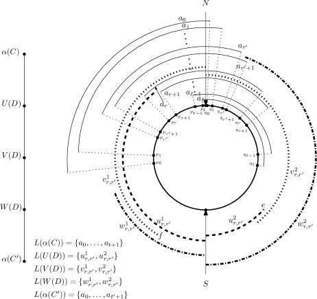
Figure 2: Construction of the graph $H_{\ell}$ and the gadgets in the proof of Lemma 13.

To define $H_{\ell}$, first fix a circle with two different points $N$ and $S$. For each ordinary clause $C$ of $F$, we introduce a vertex $\alpha(C)$ in (the top partition of) $G_{F}$. There are at most $\ell+1$ satisfying assignments of the clause $C$, and therefore we introduce $\ell+1$ arcs $a_{0},\dots,a_{\ell}$ in $H_{\ell}$ to encode all these possibilities. To define these arcs, we place $\ell+1$ points $p_{0},\dots,p_{\ell-1},p_{\ell}$ on the semicircle from $S$ to $N$ in the clockwise direction such that $p_{0}\neq S$ and $p_{\ell}\neq N$. Similarly, we place $\ell+1$ points $q_{0},q_{1},\dots,q_{\ell}$ on the semicircle from $N$ to $S$ in the clockwise direction such that $q_{0}\neq N$ and $q_{\ell}\neq S$. The arc $a_{i}$ goes from $p_{i}$ to $q_{i}$ crossing $N$, $i\in\{0,\dots,\ell\}$. See Figure 2. We call these arcs as value arcs.

Between any pair of ordinary clauses, there are at most $\ell^{2}$ possible implicational clauses. Therefore for all possible pairs $(i,j)$, $0\leq i,j\leq\ell-1$ we introduce a set of $6$ arcs in $H_{\ell}$: $u_{i,j}^{1},u_{i,j}^{2},v_{i,j}^{1},v_{i,j}^{2},w_{i,j}^{1},w_{i,j}^{2}$. The role of these sets of arcs is to simulate the implicational clauses as follows. For each implicational clause $D$ in $F$, let $C$ and $C^{\prime}$ be the two (unique) ordinary clauses associated with it. For each such $C$, $C^{\prime}$ and $D$, the graph $G_{F}$ contains a path $P=\alpha(C)-U(D)-V(D)-W(D)-\alpha(C^{\prime})$. The clauses $C$ and $C^{\prime}$ will determine the lists of $\alpha(C)$ and $\alpha(C^{\prime})$. The clause $D$ will determine $i$ and $j$, and $i$ and $j$ determine the lists of $U(D),V(D)$ and $W(D)$: $L(U(D))=\{u_{i,j}^{1},u_{i,j}^{2}\}$, $L(V(D))=\{v_{i,j}^{1},v_{i,j}^{2}\}$ and $L(W(D))=\{w_{i,j}^{1},w_{i,j}^{2}\}$.

Suppose that $C=x_{0}\rightarrow\cdots\rightarrow x_{t}$, $C^{\prime}=y_{0}\rightarrow\cdots\rightarrow y_{t^{\prime}}$, and $D=x_{r}\rightarrow y_{r^{\prime}}$. We set the list of $\alpha(C)$ to be $\{a_{0},\dots,a_{t+1}\}$, and the list of $\alpha(C^{\prime})$ to $\{a_{0},\dots,a_{t^{\prime}+1}\}$. Finally, we define the lists of $U(D),V(D)$ and $W(D)$. We set the list of $U(D)$ to be $\{u_{r,r^{\prime}}^{1},u_{r,r^{\prime}}^{2}\}$, where $u_{r,r^{\prime}}^{1}$ is an arc in $H_{\ell}$ that starts at $S$, and goes clockwise to include $p_{r}$ but not $p_{r+1}$. The arc $u_{r,r^{\prime}}^{2}$ starts at $S$ and goes anticlockwise to a point $e$ but it does not include $q_{\ell}$. Arc $v_{r,r^{\prime}}^{2}$ starts at $N$ and goes clockwise until it includes $e$ (but not $S$). Arc $v_{r,r^{\prime}}^{1}$ starts at $N$, it goes anticlockwise to a point $f$ that is (strictly) between $p_{0}$ and $S$. The arc $w_{r,r^{\prime}}^{1}$ starts at $S$ and goes clockwise until it includes $f$ but not $p_{0}$. Finally, $w_{r,r^{\prime}}^{2}$ starts at $S$ and goes anticlockwise until includes $q_{r^{\prime}+1}$ but not $q_{r^{\prime}}$.

Assume now that $\alpha(C)$ is mapped to a value arc $a_{i}$ such that $i\leq r$. Then $a_{i}$ intersects $u_{r,r^{\prime}}^{1}$, so $U(D)$ must be mapped to $u_{r,r^{\prime}}^{2}$. The arc $u_{r,r^{\prime}}^{2}$ intersects $v_{r,r^{\prime}}^{2}$, so $V(D)$ must be mapped to $v_{r,r^{\prime}}^{1}$ which in turn intersects $w_{r,r^{\prime}}^{1}$, so $W(D)$ must be mapped to $w_{r,r^{\prime}}^{2}$. The arc $w_{r,r^{\prime}}^{2}$ intersects any value arc $a_{i^{\prime}}$ such that $i^{\prime}>r^{\prime}$, so $\alpha(C^{\prime})$ must be mapped to an arc $a_{i^{\prime}}$ such that $i^{\prime}\leq r^{\prime}$.

On the other hand, if $\alpha(C)$ is mapped to a value arc $a_{i}$ such that $i>r$, then the above “chain reaction” is not triggered, so $\alpha(C^{\prime})$ can be mapped to any vertex in its list. More precisely, $U(D)$ can be mapped to $u_{r,r^{\prime}}^{1}$, $V(D)$ can be mapped to $v_{r,r^{\prime}}^{2}$, and $W(D)$ can be mapped to $w_{r,r^{\prime}}^{1}$, which does not intersect any of the value arcs, so $\alpha(C^{\prime})$ can be mapped to anything in its list.

The above analysis suggests the following correspondence between variable assignments of $F$ and homomorphisms from $G_{F}$ to $H_{\ell}$. Mapping $\alpha(C)$ to $a_{i}$ precisely corresponds to the assignment $x_{0}=\dots=x_{i-1}=0$, $x_{i}=\dots=x_{q}=1$ of the variables of $C$. It is clear that using this correspondence, given a satisfying assignment we can construct a homomorphism and vice versa. The unary clauses are encoded using the lists of the variables corresponding to ordinary clauses. For example, if $x_{i}$ is a unary clause and $x_{i}$ is among the variables of the ordinary clause $C$, then in any valid variable assignment we must have that $x_{i}=1,x_{i+1}=1,\dots,x_{q}=1$. In our interpretation, this corresponds to restricting the possible images of $\alpha(C)$ to $a_{0},a_{1},\dots,a_{i}$, so we simply remove the rest of the arcs form $L(\alpha(C))$. Similarly, if $\neg x_{i}$ is a unary clause, then we must remove $a_{j}$ from $L(\alpha(C))$ for $j\leq i$.

We give a simple example. Assume that $C=x_{0}\rightarrow x_{1}\rightarrow x_{2}\rightarrow x_{3}\rightarrow x_{4}$ and $C^{\prime}=y_{0}\rightarrow y_{1}\rightarrow y_{2}\rightarrow y_{3}$ are ordinary clauses and $D=x_{2}\rightarrow y_{2}$ is an implicational clause. Then given a satisfying variable assignment such that $x_{0}\vee x_{1}\vee x_{2}$, e.g. $x_{0}=0$ and $x_{1}=x_{2}=1$, we assign $\alpha(C)$ to $a_{1}$. Because we were given a satisfying assignment, we must have that $y_{2}=y_{3}=1$. So for example, if $y_{1}$ is the first among $y_{0},y_{1},y_{2}$ that has value $1$, then we assign $\alpha(C^{\prime})$ to $a_{1}$. We verify that this mapping can be extended to the other $3$ vertices of the path between $\alpha(C)$ and $\alpha(C^{\prime})$. Arc $a_{1}$ intersects $u_{2,2}^{1}$, so $U(D)$ can be assigned (only) to $u_{2,2}^{2}$. Then $V(D)$ can be assigned (only) to $v_{2,2}^{1}$, and $W(D)$ (only) to $w_{2,2}^{2}$, which intersects $a_{3}$. Therefore $\alpha(C^{\prime})$ can be assigned to any of $\{a_{0},a_{1},a_{2}\}$ (but not to $a_{3}$ or $a_{4}$), corresponding to the three possible ways the variables of $C^{\prime}$ could be assigned. If $y_{1}$ is the first having value $1$, then we assign $\alpha(C^{\prime})$ to $a_{1}$.

On the other hand, if $x_{0}\vee x_{1}\vee x_{2}$ is false, then we assign $\alpha(C)$ to $a_{i}$ where $x_{i}$ is the first variable in $C$ with value $1$, or if all the variables have value $0$, then $i=5$. In all these cases, the first variable among $y_{0},y_{1},y_{2},y_{3}$ that has value $1$ could be any of these variables, or all variables could be assigned $0$. If the first variable that has value $1$ is $y_{j}$, then we assign $\alpha(C^{\prime})$ to $a_{j}$. If all variables are $0$, we assign $\alpha(C^{\prime})$ to $a_{4}$. We can check that this mapping can be extended to the variables of the path between $\alpha(C)$ and $\alpha(C^{\prime})$.

For the converse, $\alpha(C)$ and $\alpha(C^{\prime})$ are prevented by the path between them to be assigned to value arcs that encode a variable assignment violating the clauses $C$ and $C^{\prime}$. If $\alpha(C)$ is mapped to $a_{i}$ where $i\leq 2$ (i.e. all those cases where $x_{2}$ has value $1$), then there is no homomorphism that maps $\alpha(C^{\prime})$ to $a_{3},a_{4}$ or $a_{5}$.

There is one more step in to complete the construction of $G_{F}$ because we want only vertices corresponding to ordinary clauses to be allowed to be removed. That is, we want to allow only vertices of the form $\alpha(C)$ or $\alpha(C^{\prime})$ to be removed. To achieve this, for every path $\alpha(C)-U(D)-V(D)-W(D)-\alpha(C^{\prime})$ we make the inner vertices “undeletable” as follows. We replace $U(D)$, $V(D)$, and $W(D)$ with $k+1$ copies. The copies inherit the lists. We add an edge between $\alpha(C)$ and any copy of $U(D)$, an edge between any copy of $U(D)$ and any copy of $V(D)$, an edge between any copy of $V(D)$ and any copy of $W(D)$, and an edge between any copy of $W(D)$ and $\alpha(C^{\prime})$. This obviously works.

Now we check that the parameters are preserved, i.e., that there is a satisfying assignment of the formula $F$ after removing the variables corresponding to $k$ ordinary clauses if and only if there is a homomorphism from $G_{F}$ to $H_{\ell}$ after removing $k$ vertices. Clearly, if after removing $k$ vertices there is a homomorphism from $G_{F}$ to $H_{\ell}$, then we can remove the ordinary clauses from the formula and use the homomorphism to define a satisfying assignment.

Conversely, if there is a satisfying assignment after removing $k$ ordinary clauses, then we remove the corresponding vertices from $G_{F}$ and define a homomorphism from the satisfying assignment. To do this, note that if either endpoint of a path $\alpha(C)-U(D)-V(D)-W(D)-\alpha(C^{\prime})$ is removed, say $\alpha(C^{\prime})$, then for any assignment of the remaining end vertex (e.g. $\alpha(C)$), we can find images for the vertices $U(D)$, $V(D)$ and $W(D)$ such that each edge of $\alpha(C)-U(D)-V(D)-W(D)$ is mapped to an edge of $H_{\ell}$. Clearly, this argument also works when we work with the copies of the inner vertices instead of the originals.

$G_{F}$ is obviously “fixed side”. Since $H_{\ell}$ has a single component, $G_{F}$ is also “fixed component”. (Observing that $w_{r,r^{\prime}}^{1}$ and $u_{r,r^{\prime}}^{2}$ are connected to all the value arcs easily gives that $H_{\ell}$ is connected.)

∎

For the converse direction, the following lemma reduces the special case FS($H$) to $\ell$-VDCS, where FS($H$) is the relaxation of the problem FS-FC($H$) where a list could contain vertices from more than one component of $H$. Note that the chain of reductions in Section 3 works for any bipartite graph $H$ (not only for skew decomposable bipartite graphs). Thus putting the two reductions together reduced a general instance of DL-Hom(${H}$) to $\ell$-VDCS.

Lemma 14

Let $H$ be a bipartite graph whose complement is a circular arc graph. Then there is a parameterized reduction from FS($H$) to $\ell$-VDCS, where $\ell=|V(H)|+1$.

Proof

Let $G$ be an instance of the fixed side problem with bipartition classes $T$ and $B$, and assume we are given a representation of $H$ as in Definition 12, where the special points on the circle are $N$ and $S$. Let $u\in T$. Clearly, we can assume that no arc $a\in L(u)$ contains any other arc in $L(u)$. Suppose that $t=|L(u)|$, and that the arcs in $L(u)$ are $a_{0},\dots,a_{t-1}$ (recall that these arcs contain $N$ but not $S$). Furthermore, let $p_{i}$ and $q_{i}$ be points on the circle such that arc $a_{i}$ is the segment of the circle that begins at $p_{i}$, goes clockwise passing $N$, and ends at point $q_{i}$. By renaming the arcs if necessary, we can assume that when we traverse the circle in the clockwise direction starting at $p_{t-1}$, we visit the endpoints of the arcs in $L(u)$ in the order $p_{t-1},p_{t-2},\dots,p_{0},q_{t-1},q_{t-2},\dots,q_{0}$. See Figure 3 for an example. Similarly, let $v\in B$ and $t^{\prime}=|L(v)|$. Let the arcs in $L(v)$ be $b_{0},\dots,b_{t^{\prime}-1}$, and suppose that $r_{i}$ and $s_{i}$ are points on the circle such that the arc obtained by going from $r_{i}$ to $s_{i}$ in the anticlockwise direction (thus traversing $S$) is precisely the arc $b_{i}$. Just as before, we assume that traversing the circle in the anticlockwise direction starting at $r_{0}$, we visit the endpoints of the arcs in $L(u)$ in the order $r_{0},r_{1},\dots,r_{t^{\prime}-1},s_{0},s_{1},\dots,s_{t^{\prime}-1}$.

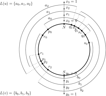
Figure 3: The graph $H$ in the proof of Lemma 3.

For a vertex $u\in T$, we introduce $t+1$ ($t=|L(u)|$) variables $x_{0},\dots,x_{t}$ in our VDCS instance. Arc $a_{i}$ is associated with the pair $(x_{i},x_{i+1})$. We add the chain clause $x_{0}\rightarrow\cdots\rightarrow x_{t}$, and the unary clauses $\neg x_{0}$, $x_{t}$. Notice that if these clauses are satisfied by a variable assignment, then there is a unique index $i$ such that $x_{i}=0$ and $x_{i+1}=1$. Intuitively, this $0-1$ transition indicates that vertex $u$ of $G$ is assigned to $a_{i}$. Any vertex $v\in B$ is handled in a similar fashion, i.e. we introduce a chain clause $y_{0}\rightarrow\dots\rightarrow y_{t^{\prime}}$ and unary clauses $\neg y_{0}$ and $y_{t^{\prime}}$, where $t^{\prime}=|L(v)|$. See Figure 3. In the VDCS instance, we will need to allow all these chain clauses to be removed, and at this point, it is possible that some of these clauses have length $2$. To remedy this, for any chain clause $z_{0}\rightarrow z_{1}$ of length $2$ introduced to represent a vertex of $G$, we add a new variable to the clause, i.e. $z_{0}\rightarrow z_{1}$ is replaced with $z_{0}\rightarrow z_{1}\rightarrow w$, for a new variable $w$. Since $z_{1}$ must always be assigned $1$ in a satisfying assignment, $w$ must also always be assigned value $1$, so the presence of $w$ does not affect in our formula in any way, except that now $z_{0}\rightarrow z_{1}\rightarrow w$ is allowed to be removed according to the definition of VDCS. (Note that adding a variable to chain clauses of length $2$ to make them length $3$ could result in a $3$-VDCS instance, where $|V(H)|+1=2$. In this case, $|V(H)|=1$, so we can just solve the problem directly.)

We define clauses to encode that edges of $G$ must be mapped to edges of $H$. Let $\{u,v\}$ be an edge of $G$. We interpret $x_{i}=1$ as $u$ being assigned to one of $a_{0},\dots,a_{i-1}$, and $x_{i}=0$ as $u$ being assigned to one of $a_{i},\dots,a_{t-1}$. Similarly for $v\in B$, $y_{j}=1$ is interpreted as assigning $v$ to one of $b_{0},\dots,b_{j-1}$, and $y_{j}=0$ as $v$ being assigned to $b_{j},\dots,b_{t^{\prime}-1}$.

We introduce two sets of implicational clauses, the first one consisting of $t$ clauses, and the second one consisting of $t^{\prime}$ clauses. The role of the first set is to ensure that if $u$ is mapped to an arc $a_{i}$, then $v$ is mapped to an arc $b_{j}$ that does not intersect $a_{i}$ on the arc from $N$ to $S$ in the clockwise direction. The role of the second set is to ensure that if $v$ is mapped to an arc $b_{j}$, then $u$ is mapped to an arc $a_{i}$ that does not intersect $b_{j}$ on the arc from $N$ to $S$ in the anticlockwise direction. We define the first set only, as the second set is defined analogously.

The first set of implicational clauses are $x_{i}\rightarrow y_{j_{i}}$, one for each $i\in\{1,\dots,t\}$, where $j_{i}$ is defined as follows. Let $j^{\prime}$ be the largest integer such that we can get from $q_{i-1}$ to $s_{j^{\prime}}$ on the circle in the clockwise direction without crossing $S$. Then $j_{i}=j^{\prime}+1$. In Figure 3, this corresponds to finding the “outermost” arc containing $S$ that “still” does not intersect $a_{i-1}$. For example, let $i=2$ in Figure 3. Then $j_{i}=2$, and we obtain the implicational clause $x_{2}\rightarrow y_{2}$. The rest of the implicational clauses in the figure are $x_{1}\rightarrow y_{1}$ and $x_{3}\rightarrow y_{3}$. In the example in the figure, the second set of implicational clauses are $y_{1}\rightarrow x_{1}$, $y_{2}\rightarrow y_{1}$, and $y_{3}\rightarrow x_{3}$.

If we have a homomorphism $h$ from $G$ to $H$, we can construct a satisfying assignment for the VDCS formula by setting the variables as suggested above. That is, if vertex $u$ is in the bipartite class $T$ of $G$ and $u$ is mapped to an arc $a_{i}(u)\in L(u)$ then we set $x_{j}=0$ for all $j\leq i$, and $x_{j}=1$ for all $j>i$. We similarly set the values of the variables of any chain clause associated with a vertex in the bipartite class $B$ of $G$. Notice that this assignment automatically satisfies all the chain clauses.

Consider an arbitrary implicational clause $x_{i}\rightarrow y_{j}$, where $x_{i}$ is a variable in a chain clause associated with a vertex $u\in T$, and $y_{j}$ is a variable associated with a vertex $v\in B$. For the sake of contradiction, assume that $x_{i}=1$ and $y_{j}=0$. The way we assigned the values of the variables indicates that $h(u)\in\{a_{0},\dots,a_{i-1}\}$, and $v\in\{b_{j},\dots,b_{t^{\prime}}\}$. But because the clause $x_{i}\rightarrow y_{j}$ exists, we know that $\{u,v\}$ is an edge of $G$, so we conclude from the definition of $x_{i}\rightarrow y_{j}$ that each arc $a_{0},\dots,a_{i-1}$ is intersected by the arc $b_{j}$, and also by each of $b_{j+1},\dots,b_{t^{\prime}}$ because of the ordering of the arcs. This contradicts the fact that $h$ is a homomorphism.

Conversely, assume that the VDCS formula is satisfied. Then for each vertex of $u\in T$, we find the (unique) index $i$ of the chain clause associated with $u$ such that $x_{i}=0$ and $x_{i+1}=1$, and we define $h(u)$ to be $a_{i}$. We similarly define the images of vertices in $B$. To see that $h$ is a homomorphism, assume for the sake of contradiction that an edge $\{u,v\}$ of $G$ is assigned to a non-edge of $H$. Let $a$ and $b$ be the arcs to which $u$ and $v$ are assigned, respectively, and let $x_{0},\dots,x_{t}$ and $y_{0},\dots,y_{t^{\prime}}$ be the variables associated with $u$ and $v$, respectively. Then for some $i$ and $j$, we have that $x_{i}=0,x_{i+1}=1$ and $y_{j}=0,y_{j+1}=1$, from our definition of mapping the vertices of $G$ to $V(H)$, we have that $a=a_{i}$ and $b=b_{j}$. Assume without loss of generality that $a_{i}$ and $b_{j}$ intersect on the semi-circle from $N$ to $S$ going in the clockwise direction. Find the smallest $j^{\prime}$ such that $b_{j^{\prime}}$ intersects $a_{i}$ on the semi-circle from $N$ to $S$ going in the clockwise direction. Then by definition, the implicational clause $x_{i+1}\rightarrow y_{j^{\prime}}$ is present in the VDCS. Since the formula is satisfied, $y_{j^{\prime}}=1$, and because $j^{\prime}\leq j$, therefore $y_{j}=1$, a contradiction.

For the parameters, if there is a homomorphism from $G$ to $H$ after removing $k$ vertices $v_{1},\dots,v_{k}$, then the $\ell^{\prime}$-VDCS formula obtained by removing the variables of the chain clauses associated with $v_{1},\dots,v_{k}$ gives exactly the formula obtained from $G[V(G)\setminus\{v_{1},\dots,v_{k}\}]$ directly. The converse works similarly. ∎

5 Concluding Remarks

The list homomorphism problem is a widely investigated problem in classical complexity theory. In this work, we initiated the study of this problem from the perspective of parameterized complexity: we have shown that the DL-Hom(${H}$) is FPT for any skew decomposable graph $H$ parameterized by the solution size and $|H|$, an algorithmic meta-result unifying the fixed parameter tractability of some well-known problems. To achieve this, we welded together a number of classical and recent techniques from the FPT toolbox in a novel way. Our research suggests many open problems, four of which are:

1. If $H$ is a fixed bipartite graph whose complement is a circular arc graph, is DL-Hom(${H}$) FPT parameterized by solution size? (Conjecture 1.1.)

2. If $H$ is a fixed digraph such that L-Hom(${H}$) is in logspace (such digraphs have been recently characterised in [6]), is DL-Hom(${H}$) FPT parameterized by solution size?

3. If $H$ is a matching consisting of $n$ edges, is DL-Hom(${H}$) FPT, where the parameter is only the size of the deletion set?

4. Consider DL-Hom(${H}$) for target graphs $H$ in which both vertices with and without loops are allowed. It is known that for such target graphs L-Hom(${H}$) is in P if and only if $H$ is a bi-arc graph [10], or equivalently, if and only if $H$ has a majority polymorphism. If $H$ is a fixed bi-arc graph, is there an FPT reduction from DL-Hom(${H}$) to $\ell$-CDCS, where $\ell$ depends only on $|H|$?

Note that for the first problem, we already do not know if DL-Hom(${H}$) is FPT when $H$ is a path on 7 vertices. (If $H$ is a path on 6 vertices, there is a simple reduction to Almost 2-SAT once we ensure that the instance has fixed side lists.) Observe that the third problem is a generalization of the Vertex Multiway Cut problem parameterized only by the cutset. For the fourth problem, we note that the FPT reduction from DL-Hom(${H}$) to CDCS for graphs without loops relies on the fixed side nature of the lists involved. Since the presence of loops in $H$ makes the concept of a fixed side list meaningless, it is not clear how to achieve such a reduction.

References

- [1] R. H. Chitnis, M. Cygan, M. Hajiaghayi, and D. Marx. Directed subset feedback vertex set is fixed-parameter tractable. In ICALP (1), 2012.
- [2] R. H. Chitnis, M. Hajiaghayi, and D. Marx. Fixed-parameter tractability of directed multiway cut parameterized by the size of the cutset. In SODA, 2012.
- [3] B. Courcelle. Graph rewriting: An algebraic and logic approach. In J. van Leeuwen, editor, Handbook of Theoretical Computer Science: Volume B: Formal Models and Semantics, pages 193–242. Elsevier, Amsterdam, 1990.
- [4] M. Cygan, M. Pilipczuk, M. Pilipczuk, and J. O. Wojtaszczyk. On multiway cut parameterized above lower bounds. In IPEC, pages 1–12, 2011.
- [5] R. G. Downey and M. R. Fellows. Parameterized Complexity. Springer-Verlag, 1999.
- [6] L. Egri, P. Hell, B. Larose, and A. Rafiey. Space complexity of list H-colouring: a dichotomy. CoRR, abs/1308.0180, 2013.
- [7] L. Egri, A. A. Krokhin, B. Larose, and P. Tesson. The complexity of the list homomorphism problem for graphs. Theory of Computing Systems, 51(2):143–178, 2012.
- [8] T. Feder and P. Hell. List homomorphisms to reflexive graphs. J. Comb. Theory, Ser. B, 72(2):236–250, 1998.
- [9] T. Feder, P. Hell, and J. Huang. List homomorphisms and circular arc graphs. Combinatorica, 19(4):487–505, 1999.
- [10] T. Feder, P. Hell, and J. Huang. Bi-arc graphs and the complexity of list homomorphisms. Journal of Graph Theory, 42(1):61–80, 2003.
- [11] T. Feder, P. Hell, and J. Huang. List homomorphisms of graphs with bounded degrees. Discrete Mathematics, 307:386–392, 2007.
- [12] T. Feder and M. Y. Vardi. The computational structure of monotone monadic SNP and constraint satisfaction: A study through datalog and group theory. SIAM J. Comput., 28(1):57–104, 1998.
- [13] J. Flum and M. Grohe. Parameterized Complexity Theory. Springer-Verlag, 2006.
- [14] G. Gutin, A. Rafiey, and A. Yeo. Minimum cost and list homomorphisms to semicomplete digraphs. Discrete Applied Mathematics, 154:890–897, 2006.
- [15] P. Hell and J. Nešetřil. Graphs and homomorphisms. Oxford University Press, 2004.
- [16] P. Hell and J. Nešetřil. On the complexity of -coloring. Journal of Combinatorial Theory, Series B, 48:92–110, 1990.
- [17] P. Hell and A. Rafiey. The dichotomy of list homomorphisms for digraphs. In SODA, pages 1703–1713, 2011.
- [18] S. Kratsch, M. Pilipczuk, M. Pilipczuk, and M. Wahlström. Fixed-parameter tractability of multicut in directed acyclic graphs. In ICALP (1), 2012.
- [19] D. Lokshtanov and D. Marx. Clustering with local restrictions. Inf. Comput., 222:278–292, 2013.
- [20] D. Lokshtanov, N. S. Narayanaswamy, V. Raman, M. S. Ramanujan, and S. Saurabh. Faster parameterized algorithms using linear programming. CoRR, abs/1203.0833, 2012.
- [21] D. Lokshtanov and M. S. Ramanujan. Parameterized tractability of multiway cut with parity constraints. In ICALP (1), pages 750–761, 2012.
- [22] D. Marx. Parameterized graph separation problems. Theor. Comput. Sci., 351(3):394–406, 2006.
- [23] D. Marx, B. O’Sullivan, and I. Razgon. Finding small separators in linear time via treewidth reduction. CoRR, abs/1110.4765, 2011.
- [24] D. Marx and I. Razgon. Fixed-parameter tractability of multicut parameterized by the size of the cutset. CoRR, abs/1010.3633, 2010.
- [25] R. Niedermeier. Invitation to Fixed-Parameter Algorithms. Oxford University Press, 2006.
- [26] I. Razgon and B. O’Sullivan. Almost 2-SAT is fixed-parameter tractable. J. Comput. Syst. Sci., 75(8):435–450, 2009.
- [27] B. A. Reed, K. Smith, and A. Vetta. Finding odd cycle transversals. Oper. Res. Lett., 32(4):299–301, 2004.
- [28] J. Spinrad. Circular-arc graphs with clique cover number two. J. Comb. Theory, Ser. B, 44(3):300–306, 1988.