Bohr Hamiltonian with deformation-dependent mass term for the Kratzer potential

Abstract

The Deformation Dependent Mass (DDM) Kratzer model is constructed by considering the Kratzer potential in a Bohr Hamiltonian, in which the mass is allowed to depend on the nuclear deformation, and solving it by using techniques of supersymmetric quantum mechanics (SUSYQM), involving a deformed shape invariance condition. Analytical expressions for spectra and wave functions are derived for separable potentials in the cases of $\gamma$-unstable nuclei, axially symmetric prolate deformed nuclei, and triaxial nuclei, implementing the usual approximations in each case. Spectra and $B(E2)$ transition rates are compared to experimental data. The dependence of the mass on the deformation, dictated by SUSYQM for the potential used, moderates the increase of the moment of inertia with deformation, removing a main drawback of the model.

I Introduction

In the non-relativistic Schrödinger equation usually the mass is assumed to be independent of position. However, there are certain physical systems in which, according to the experimental data, the effective mass should be position dependent. Apart from semiconductor theory, in which effective masses depending on the spatial coordinates have been used since many years BenDaniel ; Gora ; Bastard ; Zhu ; Roos ; Morrow , this is also the case in atomic nuclei, especially in the collective model of Bohr Bohr .

If the mass is position dependent, then it does not commute with the momentum. Therefore there are many ways to generalize the usual form of the kinetic energy in order to obtain a Hermitian operator. In Ref. Roos , the most general non-relativistic Schrödinger equation which possesses a position dependent mass and at the same time respects hermiticity was proposed. A further step was taken in Refs. QT4267 ; Q2929 , in which a general scheme was proposed, through the introduction of a parameter $a$ in the kinetic energy term, which apart from hermiticity also ensures the exact solvability of the relevant non-relativistic Schrödinger equation, in which the mass dependence on the position is reflected in the parameter $a$.

In the realm of nuclear physics, the need for three different mass coefficients in the low lying collective bands of well-deformed axially symmetric even-even nuclei has been demonstrated using the experimental data for spectra and $B(E2)$ transition rates by Jolos and von Brentano Jolos76 ; Jolos77 ; Jolos78 . In an extended version of this approach Jolos79 ; Jolos80 a mass tensor with deformation dependent components is introduced, the method being applicable to nuclei of arbitrary shape. This approach has been recently extended to odd nuclei Erma84 ; Erma85 .

It has been recently proved DDMD that by allowing the nuclear mass to depend on the deformation, the rate of increase of the moment of inertia with deformation is moderated, thus removing a main drawback Ring of the Bohr Hamiltonian Bohr . This has been achieved by using a Davidson potential Dav and taking advantage of supersymmetric quantum mechanics (SUSYQM) techniques SUSYQM1 ; SUSYQM2 developed in the study of quantum systems with mass depending on the coordinates QT4267 ; Q2929 ; Q13107 .

It should be noticed that the Davidson potential Dav , initially introduced for the description of molecular spectra, has been used for the description of nuclei since long ago Rohoz ; EEP . A major step forward has been the clarification of its group theoretical structure when used within the Bohr Hamiltonian, which was proved to be SU(1,1)$\times$SO(5) Bahri . This breakthrough led to the development of the algebraic collective model, a very rapidly converging approach allowing the calculation of spectra and transition probabilities of nuclei of any shape Rowe735 ; Rowe753 ; Caprio ; Welsh .

In the present work we consider the deformation dependent mass (DDM) Bohr Hamiltonian with a Kratzer potential Kratzer . This potential, also used initially in molecular physics, has been first used for the description of nuclei by Fortunato and Vitturi FV1 ; FV2 . We are motivated by the following questions.

(i) It is known that in the SUSYQM framework SUSYQM1 ; SUSYQM2 ; Q2929 the functional form of the dependence of the mass on the deformation is different for each potential. A first challenge is to prove that a DDM solution exists for the Bohr Hamiltonian with a Kratzer potential, and to find the form of this functional dependence.

(ii) The shapes of the Davidson Dav and Kratzer Kratzer potentials, shown in Fig. 1, are similar for small values of $\beta$, where the $1/\beta^{2}$ term dominates in both cases, but they differ substantially at large values of $\beta$, where the tails of the wave functions behave as $e^{-\beta^{2}/2}$ ESDPRC and $e^{-\beta/2}$ FV1 ; FV2 respectively. It is interesting to examine to what extent numerical results for spectra and $B(E2)$ transition rates are influenced by the change in the potential. The level spacings within the $\beta_{1}$ band, which are usually overestimated by collective models based on the Bohr Hamiltonian, including the DDM Davidson model, are of particular interest.

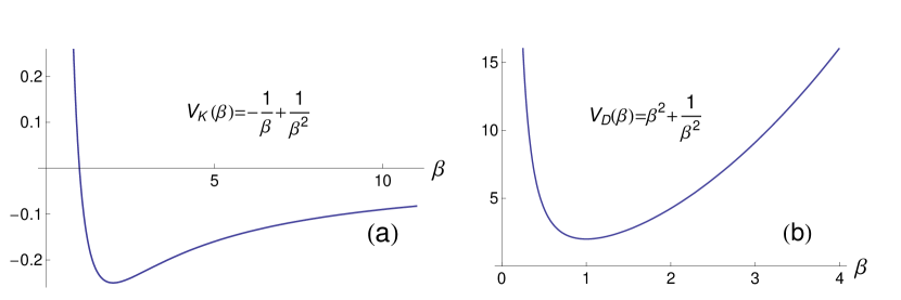
Figure 1: (Color online) The Kratzer (left) and Davidson (right) potentials. The quantities shown are dimensionless, while all free parameters have been set equal to unity, for the sake of simplicity.

(iii) The DDM Bohr Hamiltonian with the Davidson potential works well for deformed nuclei, but fails in describing the nuclei lying at the critical point between the spherical and deformed regions McCutchan ; RMP82 , known to be examples of the X(5) critical point symmetry IacX5 . It is interesting to examine if the DDM Bohr Hamiltonian with the Kratzer potential overcomes this drawback.

In Section II the DDM Bohr Hamiltonian is briefly reviewed, while in Section III the special case of the Kratzer potential is considered. Analytical expressions for spectra and wave functions are given in Sections IV and V respectively, while the calculation of $B(E2)$ transition rates is described in Section VI. Numerical results for spectra and $B(E2)$ transition rates are given in Section VII, while Section VIII contains the conclusions and plans for further work. The use of the deformed shape invariance principle for the construction of the spectrum is given in Appendix 1, while many technical details concerning the wave functions are given in Appendices 2-6. Finally, in Appendix 7, scaling factors are discussed.

II Bohr Hamiltonian with deformation-dependent mass

The original Bohr Hamiltonian Bohr is

$$H_{B}=-{\hbar^{2}\over 2B}\left[{1\over\beta^{4}}{\partial\over\partial\beta}\beta^{4}{\partial\over\partial\beta}+{1\over\beta^{2}\sin 3\gamma}{\partial\over\partial\gamma}\sin 3\gamma{\partial\over\partial\gamma}\right.$$

$$\left.-{1\over 4\beta^{2}}\sum_{k=1,2,3}{Q_{k}^{2}\over\sin^{2}\left(\gamma-{2\over 3}\pi k\right)}\right]+V(\beta,\gamma),$$ (1)

where $\beta$ and $\gamma$ are the usual collective coordinates, while $Q_{k}$ ($k=1$, 2, 3) are the components of angular momentum in the intrinsic frame, and $B$ is the mass parameter, which is usually considered constant.

Allowing the mass to depend on the deformation coordinate $\beta$ (which measures departure from spherical shape),

$$B(\beta)=\frac{B_{0}}{(f(\beta))^{2}},$$ (2)

where $B_{0}$ is a constant and $f$ a function of $\beta$ only, the Bohr equation becomes DDMD

$$\begin{split}&H\Psi=\left[-{1\over 2}{\sqrt{f}\over\beta^{4}}{\partial\over\partial\beta}\beta^{4}f{\partial\over\partial\beta}\sqrt{f}-{f^{2}\over 2\beta^{2}\sin 3\gamma}{\partial\over\partial\gamma}\sin 3\gamma{\partial\over\partial\gamma}\right.\\ &\left.+{f^{2}\over 8\beta^{2}}\sum_{k=1,2,3}{Q_{k}^{2}\over\sin^{2}\left(\gamma-{2\over 3}\pi k\right)}+v_{eff}\right]\Psi=\epsilon\Psi,\end{split}$$ (3)

where reduced energies

$$\epsilon=B_{0}E/\hbar^{2}$$ (4)

and reduced potentials

$$v=B_{0}V/\hbar^{2}$$ (5)

have been used, and DDMD

$$v_{eff}=v(\beta,\gamma)+{1\over 4}(1-\delta-\lambda)f\nabla^{2}f$$

$$+{1\over 2}\left({1\over 2}-\delta\right)\left({1\over 2}-\lambda\right)(\nabla f)^{2},$$ (6)

where $\delta$ and $\lambda$ are free parameters, stemming from the following cause. If the mass is position dependent, then it does not commute with the momentum. Therefore there are many ways to generalize the usual form of the kinetic energy in order to obtain a Hermitian operator. It was actually in Ref. Roos where it was proved that the most general form of such a Hermitian Hamiltonian contains two free parameters (denoted by $\delta$ and $\lambda$ in the present work). In Section VII it will be seen that these parameters play practically no role in the present work.

Exact separation of variables can be achieved in the usual three cases.

a) $\gamma$-unstable nuclei, in which the potential $v(\beta,\gamma)$ depends only on the variable $\beta$, i.e. $v(\beta)=u(\beta)$ Wilets ; IacE5 , and the wave functions are of the form

$$\Psi(\beta,\gamma,\theta_{i})=\xi(\beta)\Phi(\gamma,\theta_{i}),$$ (7)

where $\theta_{i}$ ($i=1$, 2, 3) are the Euler angles.

b) Axially symmetric prolate deformed nuclei with $\gamma\approx 0$, in which the potential is assumed to be of the form Wilets ; F2 ; F1 ; F3 ; ESDPRC

$$v(\beta,\gamma)=u(\beta)+{f^{2}\over\beta^{2}}w(\gamma),$$ (8)

with

$$w(\gamma)={1\over 2}(3c)^{2}\gamma^{2},$$ (9)

where $c$ is a free parameter, while the wave functions read IacX5

$$\Psi(\beta,\gamma,\theta_{i})=\xi_{L}(\beta)\eta_{K}(\gamma){\cal D}^{L}_{M,K}(\theta_{i}),$$ (10)

where ${\cal D}(\theta_{i})$ denote Wigner functions of the Euler angles, $L$ is the angular momentum quantum number, while $M$ and $K$ are the quantum numbers of the projections of angular momentum on the laboratory-fixed $z$-axis and the body-fixed $z^{\prime}$-axis respectively.

c) Triaxial nuclei with $\gamma\approx\pi/6$, in which again the potential is assumed to be of the form of Eq. (8), but with

$$w(\gamma)={1\over 4}c\left(\gamma-{\pi\over 6}\right)^{2},$$ (11)

while the wave functions read Z5

$$\Psi(\beta,\gamma,\theta_{i})=\xi_{L,\alpha}(\beta)\eta(\gamma){\cal D}^{L}_{M,\alpha}(\theta_{i}),$$ (12)

where ${\cal D}(\theta_{i})$ denote Wigner functions of the Euler angles, $L$ is the angular momentum quantum number, while $M$ and $\alpha$ are the quantum numbers of the projections of angular momentum on the laboratory-fixed $z$-axis and the body-fixed $x^{\prime}$-axis respectively.

The angular equations and wave functions can be found in Ref. DDMD . The radial equations in all three cases take the common form DDMD

$$HR(\beta)=-\left(\sqrt{f}{d\over d\beta}\sqrt{f}\right)^{2}R(\beta)+2u_{eff}R(\beta)=2\epsilon R(\beta),$$ (13)

where

$$\xi(\beta)={R(\beta)\over\beta^{2}},$$ (14)

$$u_{eff}=u+{1\over 4}(1-\delta-\lambda)f\left({4f^{\prime}\over\beta}+f^{\prime\prime}\right)$$

$$+{1\over 2}\left({1\over 2}-\delta\right)\left({1\over 2}-\lambda\right)(f^{\prime})^{2}+{f^{2}+\beta ff^{\prime}\over\beta^{2}}+{f^{2}\over 2\beta^{2}}\Lambda,$$ (15)

$f^{\prime}$ ($f^{\prime\prime}$) denote the first (second) derivative of $f$, while $\Lambda$ in each case acquires the following form.

a) For $\gamma$-unstable nuclei

$$\Lambda=\tau(\tau+3),$$ (16)

with $\tau$ being the seniority quantum number Bes . The values of angular momentum $L$ occurring for each $\tau$ are provided by a well known algorithm and are listed in IA ; Wilets . Within the ground state band (gsb) one has $L=2\tau$.

b) For axially symmetric prolate deformed nuclei,

$$\Lambda={L(L+1)-K^{2}\over 3}+(6c)(n_{\gamma}+1),$$ (17)

where $n_{\gamma}$ is the quantum number related to $\gamma$-oscillations.

c) For triaxial nuclei with $\gamma\approx\pi/6$,

$$\Lambda={L(L+4)+3n_{w}(2L-n_{w})\over 4}+\sqrt{2c}\left(n_{\gamma}+{1\over 2}\right),$$ (18)

where $n_{w}=L-\alpha$ is the wobbling quantum number BM ; MtV .

III The Kratzer potential

Up to now no assumption about the specific form of the potential $u(\beta)$ and the deformation function $f(\beta)$ has been made. From the results for 3-dimensional systems reported in Ref. Q2929 , we know that for each potential a different deformation function is appropriate.

In Ref. DDMD , the Davidson potential Dav

$$u(\beta)=\beta^{2}+{\beta_{0}^{4}\over\beta^{2}},$$ (19)

where the parameter $\beta_{0}$ indicates the position of the minimum of the potential, has been considered in the framework of the Bohr Hamiltonian, the appropriate deformation function being

$$f(\beta)=1+a\beta^{2},\qquad a\ll 1.$$ (20)

Here we are going to consider the Kratzer potential Kratzer

$$u(\beta)=-\frac{1}{\beta}+\frac{\tilde{B}}{\beta^{2}},$$ (21)

for which the deformation function is expected Q2929 to be

$$f(\beta)=1+a\beta,\qquad a\ll 1.$$ (22)

Using these forms for the potential and the deformation function in Eq. (II) one obtains

$$2u_{\rm eff}=k_{0}+\frac{k_{-1}}{\beta}+\frac{k_{-2}}{\beta^{2}},\\ k_{0}=a^{2}[2(3-\delta-\lambda)+\tfrac{1}{4}(1-2\delta)(1-2\lambda)+\Lambda],\\ k_{-1}=-2+2a[(4-\delta-\lambda)+\Lambda],\\ k_{-2}=2+\Lambda+2\tilde{B},$$ (23)

where $a$ is the deforming parameter, $\delta$ and $\lambda$ are free parameters coming from the construction procedure of the kinetic energy term Roos and going to be discussed further in Section VII.A, and $\Lambda$ is the eigenvalue coming from the exact separation of variables, given by Eqs. (16), (17), (18), depending on the nature of the nucleus in discussion ($\gamma$-unstable, axially symmetric prolate deformed, triaxial with $\gamma\approx\pi/6$ respectively).

The radial equation for the Kratzer potential is solved in Appendix 1, using deformed shape invariance.

IV Energy spectrum

Using the results of Appendix 1, the energy spectrum of Eq. (13) is given by

$$\epsilon_{n}=\frac{1}{2}\left[k_{0}-\left(\frac{k_{-1}+a\left[n^{2}+\frac{1}{2}(1+\Delta)(2n+1)\right]}{2n+1+\Delta}\right)^{2}\right],\\ \qquad n=0,1,2,\ldots,$$ (24)

where

$$\Delta\equiv\sqrt{1+4k_{-2}}.$$ (25)

Equation (24) only provides a formal solution to the bound-state energy spectrum. The range of $n$ values is actually determined by the existence of corresponding physically acceptable wave functions, the relevant conditions being stated in Appendix 2.

In Eq. (24) the quantities $k_{0}$, $k_{-1}$, $k_{-2}$ are given by Eq. (23), in which $\Lambda$ is given by Eq.(16), (17), or (18), for $\gamma$-unstable, axially symmetric prolate deformed, or triaxial nuclei respectively. The ground state band is obtained for $n=0$, while for $n=1$ and $n=2$ the quasi-$\beta_{1}$ and quasi-$\beta_{2}$ bands are obtained respectively.

In the limit of no dependence of the mass on the deformation, i.e., $a\to 0$, one has from Eq. (23)

$$k_{0}=0,\qquad k_{-1}=-2.$$ (26)

In this limit the spectrum becomes

$$\epsilon_{n}=-{1\over 2\left(n+{1\over 2}+{\Delta\over 2}\right)^{2}}.$$ (27)

For $\gamma$-unstable nuclei this reads

$$\epsilon_{n}=-{1\over 2\left(n+{1\over 2}+\sqrt{\left(\tau+{3\over 2}\right)^{2}+2\tilde{B}}\right)^{2}},$$ (28)

in agreement with Eq. (11) of Ref. FV1 .

In the axially symmetric prolate deformed case the energies for the ground state and $\beta$ bands in the limit $a\to 0$ read

$$\epsilon_{n}=-{1\over 2\left(n+{1\over 2}+\sqrt{{9\over 4}+{L(L+1)\over 3}+2\tilde{B}}\right)^{2}},$$ (29)

in agreement with Eq. (10) of Ref. FV2 .

V Wave functions

The ground-state wavefunction is found in Appendix 3 to read

$$R_{0}(\beta)=N_{0}\beta^{-\mu}f^{\frac{1}{2}\left(\mu+\frac{\tilde{K}}{\mu}-1\right)},$$ (30)

where

$$\mu=-{1\over 2}(1+\Delta),$$ (31)

while the normalization factor $N_{0}$ is given by Eq. (79), and $\tilde{K}$ is given by Eq. (51).

As discussed in Appendix 3, this wave function is physically acceptable if the inequality

$$|\mu|=\frac{1}{2}(1+\Delta)<-\frac{k_{-1}}{a},$$ (32)

is satisfied by the parameters of the problem.

The excited state wave functions are found in Appendix 4 to be

$$R_{n}(\beta)=N_{n}\beta^{-\mu_{n}}f^{\frac{1}{2}\left(\mu_{n}+\frac{\tilde{K}}{\mu_{n}}-1\right)}P_{n}^{\left(\mu_{n}-\frac{\tilde{K}}{\mu_{n}},\mu_{n}+\frac{\tilde{K}}{\mu_{n}}\right)}(t),\\ \qquad t=\frac{2+a\beta}{a\beta},$$ (33)

where $\mu_{n}=\mu-n$, by $P_{n}^{(\alpha,\beta)}(t)$ the Jacobi polynomials AbrSte are denoted, while the normalization coefficient $N_{n}$ is given by Eq. (80) in Appendix 5.

The reduction of the present wave functions to the form they have in the $a\to 0$ limit FV1 ; FV2 is carried out in Appendix 6.

VI $B(E2)$ transition rates

For the calculation of $B(E2)$ transition rates, the formulae given in Section X of Ref. DDMD apply, with the wave functions $R_{n}(\beta)$ being replaced by the present results.

VII Numerical results

VII.1 Spectra of $\gamma$-unstable nuclei

Rms fits of spectra have been performed, using the quality measure

$$\sigma=\sqrt{{\sum_{i=1}^{n}(E_{i}(exp)-E_{i}(th))^{2}\over(n-1)E(2_{1}^{+})^{2}}}.$$ (34)

The same set of experimental data for spectra and $B(E2)$ transition rates has been used as in the cases of the Deformation Dependent Mass (DDM) Davidson model DDMD , the Exactly Separable Davidson (ESD) model ESDPRC , and the Morse potential MorseI ; MorseII , in order to facilitate comparisons of the various models among themselves and to the data.

The theoretical predictions for the levels are obtained from Eq. (24), the ground state band corresponding to $n=0$ and the quasi-$\beta_{1}$ band having $n=1$. The levels of the quasi-$\gamma_{1}$ band are obtained through their degeneracies to members of the ground state band, implied by the SO(5)$\supset$SO(3) reduction rules Wilets ; IA , also listed in Table I of Ref. BonE5 . Within the ground state band (gsb) one has $L=2\tau$. The $L=2$ member of the quasi-$\gamma_{1}$ band is degenerate with the $L=4$ member of the gsb, the $L=3$, 4 members of the quasi-$\gamma_{1}$ band are degenerate to the $L=6$ member of the gsb, the $L=5$, 6 members of the quasi-$\gamma_{1}$ band are degenerate to the $L=8$ member of the gsb, and so on.

The results shown in Table I have been obtained for $\delta=\lambda=0$. One can easily verify that different choices for $\delta$ and $\lambda$ lead to a renormalization of the parameter values $a$ and $\beta_{0}$, the predicted energy levels remaining exactly the same.

Concerning the physical content of the parameter $a$, it is instructive to consider in detail in Table I the Xe isotopes, known Casten to lie in the $\gamma$-unstable region and already discussed in the framework of the DDM Davidson model DDMD . They extend from the borders of the neutron shell (with ¹³⁴Xe₈₀ lying just below the N=82 shell closure) to the midshell (¹²⁰Xe₆₆) and even beyond, exhibiting increasing collectivity (increasing $R_{4/2}=E(4_{1}^{+})/E(2_{1}^{+})$ ratios) from the border to the midshell.

Moving from the border of the neutron shell to the midshell, the following remarks apply.

i) The Kratzer parameter $\tilde{B}$ is increasing smoothly as one moves from the border towards the middle of the shell.

ii) The $a$ parameter, expressing the dependence of the mass on the deformation, is zero, or close to zero, for the first 4 isotopes close to the border, while it acquires substantially non-zero values for the last 5 isotopes close to mid-shell. This indicates that for nearly spherical nuclei no dependence of the mass on the deformation is needed, while it is becoming necessary as soon as substantial deviations from the spherical shape set in.

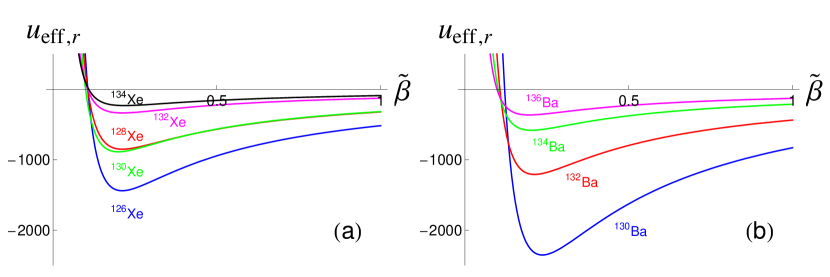
Figure 2: (Color online) Effective potentials (Eq. (23)) for $L=4$ for some Xe (a) and Ba (b) isotopes, corresponding to the parameters of Table I. The quantities shown are dimensionless. Rescaling has been carried out, according to Appendix 7, using the rescaling parameters $A$ given in Table VII. The rescaled effective potentials are given by Eq. (127), while the rescaled abscissa, $\tilde{\beta}$, is given by Eq. (111).

The effective potentials of Eq. (23) for some Xe isotopes, appropriately rescaled as described in Appendix 7, are shown in Fig. 2(a). It is clear that the potentials get deeper as one moves from the border of the neutron shell (¹³⁴Xe₈₀) to the midshell (¹²⁰Xe₆₆).

Other chains of isotopes also show similar behavior. As an example, the effective potentials of Eq. (23) for some Ba isotopes, appropriately rescaled as described in Appendix 7, are shown in Fig. 2(b). It is again clear that the potentials get deeper as one moves from the border of the neutron shell (¹³⁶Ba₈₀) towards the midshell (¹²²Ba₆₆).

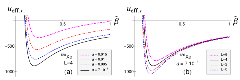
Figure 3: (Color online) Dependence of the effective potentials of Eq. (23) on the parameter $a$ [panel (a)] and on the angular momentum $L$ [panel (b)]. The quantities shown are dimensionless. The effective potential for the $L=4$ state of the ground state band of ¹³⁰Xe (corresponding to the parameters of Table I), plotted in both panels, is used as the basis of the comparison. Rescaling has been carried out, according to Appendix 7, using the rescaling parameters $A$ given in Table VII. The rescaled effective potentials are given by Eq. (127), while the rescaled abscissa, $\tilde{\beta}$, is given by Eq. (111).

The dependence of the effective potentials of Eq. (23) on the parameter $a$ and on the angular momentum $L$ is shown in Fig. 3, after appropriate rescaling according to Appendix 7. The effective potential of the $L=4$ state of the ground state band of ¹³⁰Xe is used as the basis for the comparison. It is seen that the effective potential becomes less deep as the parameter $a$ is increased. It also becomes less deep as the angular momentum $L$ is increased.

It is remarkable that all effective potentials shown in Figs. 2 and 3 look qualitatively similar to the pure Kratzer potential of Fig. 1(left).

VII.2 Spectra of axially symmetric deformed nuclei

Fits of spectra of deformed rare earth and actinide nuclei are shown in Table II. The energy levels are obtained from Eq. (24). The ground state band is obtained for $n=0$ and the $\beta_{1}$ band for $n=1$, while both have $n_{\gamma}=0$ and $K=0$. The $\gamma_{1}$ band is obtained for $n=0$, $n_{\gamma}=1$ and $K=2$. Again, the choice $\delta=\lambda=0$ has been made, and it is seen that different choices for $\delta$ and $\lambda$ lead to a renormalization of the parameter values $a$, $B$, and $c$, the predicted energy levels remaining exactly the same.

The quality of the fits obtained can also be seen in Table III, where the calculated energy levels of ¹⁷⁰Er and ²³²Th are compared to experiment.

The main discrepancy between theory and experiment in the case of the DDM Davidson DDMD was found in the $\beta_{1}$-bands, in which the theoretical level spacings were larger than the experimental ones. This was attributed to the shape of the Davidson potential, which raises to infinity at large $\beta$, pushing $\beta$ bands higher and increasing their interlevel spacing. It is known that this problem can be avoided by using a potential going to some finite value at large $\beta$ finitew , like the Morse potential Morse . The Kratzer potential is going to zero for large $\beta$, thus avoiding the problem of the overestimation of the level spacings within the $\beta_{1}$ band, as seen clearly in Table III.

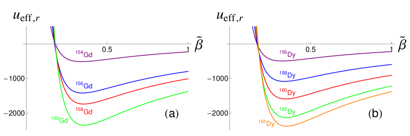
Figure 4: (Color online) Effective potentials (Eq. (23)) for $L=4$ for some Gd (a) and Dy (b) isotopes, corresponding to the parameters of Table II. The quantities shown are dimensionless. Rescaling has been carried out, according to Appendix 7, using the rescaling parameters $A$ given in Table VIII. The rescaled effective potentials are given by Eq. (127), while the rescaled abscissa, $\tilde{\beta}$, is given by Eq. (111).

In Fig. 4 the effective potentials of Eq. (23) for some Gd and Dy isotopes, appropriately rescaled as described in Appendix 7, are shown. It is clear that the potentials get deeper as one moves from the border of the neutron shell towards the midshell.

Another difference between the DDM Davidson and the present DDM Kratzer model is that the former cannot describe the ${\rm N}=90$ isotones ¹⁵⁰Nd, ¹⁵²Sm, ¹⁵⁴Gd, and ¹⁵⁶Dy, which are considered RMP82 as the best examples of the X(5) IacX5 critical point symmetry, while in the latter a good description is obtained. Indeed, in Table II of Ref. DDMD one sees that large $\sigma$ deviations are obtained in the DDM Davidson case, while the spectra obtained in the present DDM Kratzer case are reported in Table IV, along with the parameter-free X(5) predictions IacX5 ; BonX5 ; Bijker . In the $\beta_{1}$ bands, in particular, we see that the present approach, using the same number of parameters (three in the case of axially deformed nuclei) as the DDM Davidson model, avoids the overestimation of the interlevel spacings.

The ability of the DDM Kratzer model to describe the $N=90$ isotones, in which the DDM Davidson model fails, can be understood by considering the shapes of the two potentials. The Kratzer potential for appropriate parameter values can acquire the shape of a deep well, thus resembling the infinite square well potential used in the X(5) model IacX5 , known to describe these ${\rm N}=90$ isotones.

In Fig. 5, the (rescaled according to Appendix 7) effective potentials for the ${\rm N}=90$ nuclei being good examples of the X(5) critical point symmetry are isolated, corroborating the remarks made above.

Figure 5: (Color online) Effective potentials (Eq. (23)) for $L=4$ for the ${\rm N}=90$ isotones being good examples of the X(5) critical point symmetry, corresponding to the parameters of Table II. The quantities shown are dimensionless. Rescaling has been carried out, according to Appendix 7, using the rescaling parameters $A$ given in Table VIII. The rescaled effective potentials are given by Eq. (127), while the rescaled abscissa, $\tilde{\beta}$, is given by Eq. (111).

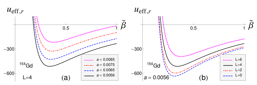
Figure 6: (Color online) Dependence of the effective potentials of Eq. (23) on the parameter $a$ [panel (a)] and on the angular momentum $L$ [panel (b)]. The quantities shown are dimensionless. The effective potential for the $L=4$ state of the ground state band of ¹⁵⁴Gd (corresponding to the parameters of Table II), plotted in both panels, is used as the basis of the comparison. Rescaling has been carried out, according to Appendix 7, using the rescaling parameters $A$ given in Table VIII. The rescaled effective potentials are given by Eq. (127), while the rescaled abscissa, $\tilde{\beta}$, is given by Eq. (111).

The dependence of the (rescaled according to Appendix 7) effective potentials of Eq. (23) on the parameter $a$ and on the angular momentum $L$ is shown in Fig. 6. The effective potential of the $L=4$ state of the ground state band of ¹⁵⁴Gd is used as the basis for the comparison. It is again seen that the effective potential becomes less deep as the parameter $a$ is increased. It also becomes less deep as the angular momentum $L$ is increased.

VII.3 $B(E2)$s of $\gamma$-unstable nuclei

$B(E2)$s within the ground state band, as well as interband $B(E2)$s for which experimental data exist for several nuclei, have been calculated using the procedure described in subsec. X.A of Ref. DDMD . For each nucleus, the parameters obtained by fitting the spectra have been used. The results are shown in Table V, the overall agreement being good.

VII.4 $B(E2)$s of axially symmetric deformed nuclei

$B(E2)$s within the ground state band, as well as interband $B(E2)$s for which experimental data exist for several nuclei, have been calculated using the procedure described in subsec. X.B of Ref. DDMD . The results are shown in Table VI. In order to facilitate comparison with the ${\rm N}=90$ isotones ¹⁵⁰Nd, ¹⁵²Sm, ¹⁵⁴Gd, and ¹⁵⁶Dy, which are considered RMP82 as the best examples of the X(5) IacX5 critical point symmetry, the X(5) predictions IacX5 ; BonX5 ; Bijker are shown in the first line of the table. The overall agreement is good, although interband transitions are usually overestimated by theory.

VIII Conclusions

The main results of the present work are summarized here.

(i) Analytical solutions of the deformation dependent mass (DDM) Bohr Hamiltonian with the Kratzer potential have been obtained for $\gamma$-unstable, axially symmetric prolate deformed, and triaxial nuclei. The deformation function for the Kratzer potential was found to be $f(\beta)=1+a\beta$, to be compared with the deformation function $f(\beta)=1+a\beta^{2}$ obtained in the case of the Davidson potential DDMD .

(ii) Despite the fact that the Davidson and Kratzer potentials have very different shapes, numerical results coming from fitting the spectra of more than 100 nuclei and then using the same parameters for calculating $B(E2)$ transition rates, indicate that good overall agreement to the experimental data is achieved in both cases. Therefore the important factor in obtaining spectra with proper dependence of the moment of inertia on the deformation is the dependence of the mass on the deformation, independently of the particular shape of the potential.

(iii) On the other hand, a substantial difference between the two potentials shows up in the level spacings within the $\beta_{1}$ band. While these spacings are usually overestimated by collective models based on the Bohr Hamiltonian, the DDM Davidson model included, the present DDM Kratzer model avoids this problem, using the same number of parameters as the DDM Davidson model.

(iv) Furthermore, the Kratzer potential is able to acquire the shape of a deep narrow well, while the Davidson potential cannot achieve this. As a result, the DDM Bohr Hamiltonian with the Kratzer potential succeeds in describing the ${\rm N}=90$ rare earths which are considered as hallmark examples McCutchan ; RMP82 of the X(5) critical point symmetry IacX5 between spherical and deformed nuclei.

The physical content of the free parameter $a$ appearing in the dependence of the mass on the deformation can be further investigated in at least two ways:

(i) By exploiting the equivalence of the deformation dependence of the mass to a curved space QT4267 .

(ii) By considering the similarity of several terms appearing in the DDM Bohr Hamiltonian to the Hamiltonian of the classical limit GK of the interacting boson model IA .

Work in these directions is in progress.

Appendix 1: Deformed shape invariance

$H$ may be considered as the first member $H_{0}=H$ of a hierarchy of Hamiltonians

$$H_{i}=A_{i}^{+}A_{i}^{-}+\sum_{j=0}^{i}\varepsilon_{j},\qquad i=0,1,2,\ldots,$$ (35)

where the first-order operators Q2929

$$A_{i}^{\pm}=A^{\pm}(\mu_{i},\nu_{i})=\mp\sqrt{f}\frac{d}{d\beta}\sqrt{f}+W(\mu_{i},\nu_{i};\beta)$$ (36)

satisfy a deformed shape invariance condition

$$A_{i}^{-}A_{i}^{+}=A_{i+1}^{+}A_{i+1}^{-}+\varepsilon_{i+1},\qquad i=0,1,2,\ldots,$$ (37)

with $\varepsilon_{i}$, $i=0$, 1, 2, …, denoting some constants. In other words, the superpotential $W(\mu,\nu;\beta)$ fulfils the two conditions

$$W^{2}(\mu,\nu;\beta)-f(\beta)W^{\prime}(\mu,\nu;\beta)+\varepsilon_{0}=2u_{\rm eff}(\beta),$$ (38)

and

$$W^{2}(\mu_{i},\nu_{i};\beta)+f(\beta)W^{\prime}(\mu_{i},\nu_{i};\beta)=\\ W^{2}(\mu_{i+1},\nu_{i+1};\beta)-f(\beta)W^{\prime}(\mu_{i+1},\nu_{i+1};\beta)+\varepsilon_{i+1},\\ i=0,1,2,\ldots,$$ (39)

where $\mu_{0}=\mu$, $\nu_{0}=\nu$, and a prime denotes derivative with respect to $\beta$.

In the case of the effective potential given in Eq. (23), $W(\mu,\nu;\beta)$ is a class 1 superpotential

$$W(\mu,\nu;\beta)=\mu\phi(\beta)+\nu,$$ (40)

$$\phi(\beta)=\frac{1}{\beta},$$ (41)

which means that Eqs. (3.9) and (3.10) of Q2929 read

$$\begin{split}&\phi^{\prime}(\beta)=-\frac{1}{\beta^{2}}=\frac{A}{\beta^{2}}+\frac{B}{\beta}+C,\\ &a\beta=\frac{(A^{\prime}/\beta^{2})+(B^{\prime}/\beta)+C^{\prime}}{(-1/\beta^{2})},\end{split}$$ (42)

with $A=-1$, $B=C=0$, $A^{\prime}=0$, $B^{\prime}=-a$ and $C^{\prime}=0$.

Inserting Eqs. (40) and (41) in (38), we obtain

$$\left(\frac{\mu}{\beta}+\nu\right)^{2}-(1+a\beta)\left(-\frac{\mu}{\beta^{2}}\right)+\varepsilon_{0}=k_{0}+\frac{k_{-1}}{\beta}+\frac{k_{-2}}{\beta^{2}},$$ (43)

which is equivalent to the three equations

$$\mu(\mu+1)=k_{-2},\quad\mu(2\nu+a)=k_{-1},\quad\nu^{2}+\varepsilon_{0}=k_{0}.$$ (44)

Their solutions read

$$\begin{split}&\mu=\frac{1}{2}(-1\pm\Delta),\qquad\nu=\frac{k_{-1}-a\mu}{2\mu},\qquad\varepsilon_{0}=k_{0}-\nu^{2},\\ &\Delta\equiv\sqrt{1+4k_{-2}},\end{split}$$ (45)

where we note that $1+4k_{-2}$ is always positive. As we shall show in Appendix 2, the conditions ensuring that the ground state wavefunction is physically acceptable select the lower sign for $\mu$:

$$\mu=-\frac{1}{2}(1+\Delta).$$ (46)

Inserting next Eqs. (40) and (41) in Eq. (39), we get

$$\left(\frac{\mu_{i}}{\beta}+\nu_{i}\right)^{2}+(1+a\beta)\left(-\frac{\mu_{i}}{\beta^{2}}\right)=\\ \left(\frac{\mu_{i+1}}{\beta}+\nu_{i+1}\right)^{2}-(1+a\beta)\left(-\frac{\mu_{i+1}}{\beta^{2}}\right)+\varepsilon_{i+1},$$ (47)

leading to the three conditions

$$\begin{split}&\mu_{i}(\mu_{i}-1)=\mu_{i+1}(\mu_{i+1}+1),\\ &\mu_{i}(2\nu_{i}-a)=\mu_{i+1}(2\nu_{i+1}+a),\\ &\nu_{i}^{2}=\nu_{i+1}^{2}+\varepsilon_{i+1}.\end{split}$$ (48)

Their solutions are

$$\mu_{i+1}=\mu_{i}-1,\qquad 2\mu_{i+1}\nu_{i+1}=2\mu_{i}\nu_{i}-a(\mu_{i}+\mu_{i+1}),\\ \varepsilon_{i+1}=\nu_{i}^{2}-\nu_{i+1}^{2}.$$ (49)

Note that there is an other solution for $\mu_{i+1}$, namely $\mu_{i+1}=-\mu_{i}$, but the alternating signs would not be compatible with physically acceptable excited state wave functions. Finally, the iteration of the first two relations in (49) leads to

$$\mu_{i}=\mu-i,\qquad\nu_{i}=\frac{2\mu(\nu-ai)+ai^{2}}{2(\mu-i)}.$$ (50)

For future use, it is worth observing that $\nu_{i}$ can be rewritten in terms of $\mu_{i}$ as

$$\nu_{i}=\frac{a}{2}\left(\mu_{i}-\frac{\tilde{K}}{\mu_{i}}\right),\qquad\tilde{K}\equiv k_{-2}-\frac{k_{-1}}{a}.$$ (51)

From (50), it indeed follows that

$$\nu_{i}=\frac{a}{2}\left(\mu_{i}-\frac{\mu\left(\mu-\frac{2\nu}{a}\right)}{\mu_{i}}\right),$$ (52)

while Eq. (44) leads to

$$k_{-2}-\frac{k_{-1}}{a}=\mu\left(\mu-\frac{2\nu}{a}\right).$$ (53)

The energy spectrum of Eq. (13) is therefore given by

$$\epsilon_{n}=\tfrac{1}{2}\sum_{i=0}^{n}\varepsilon_{i}=\tfrac{1}{2}\left(k_{0}-\nu_{n}^{2}\right)\\ =\frac{1}{2}\left[k_{0}-\left(\frac{k_{-1}+a\left[n^{2}+\frac{1}{2}(1+\Delta)(2n+1)\right]}{2n+1+\Delta}\right)^{2}\right],\\ n=0,1,2,\ldots.$$ (54)

Appendix 2: Conditions for physically acceptable wave functions

To be physically acceptable, the bound-state wavefunctions should satisfy two conditions Q2929 :

(i) As in conventional (constant-mass) quantum mechanics, they should be square integrable on the interval of definition of $u_{\rm eff}$, i.e.,

$$\int_{0}^{\infty}d\beta\,|R_{n}(\beta)|^{2}<\infty.$$ (55)

(ii) Furthermore, they should ensure the Hermiticity of $H$. For such a purpose, it is enough to impose that the operator $-{\rm i}\sqrt{f}(d/d\beta)\sqrt{f}$ be Hermitian, which amounts to the restriction

$$|R_{n}(\beta)|^{2}f(\beta)\to 0\qquad{\rm for\ }\beta\to 0{\rm\ and\ }\beta\to\infty,$$ (56)

or, equivalently,

$$|R_{n}(\beta)|^{2}\to 0\quad{\rm for\ }\beta\to 0\qquad{\rm and}\\ \qquad|R_{n}(\beta)|^{2}\beta\to 0\quad{\rm for\ }\beta\to\infty.$$ (57)

As condition (57) is more stringent than condition (55), we should only be concerned with the former.

Appendix 3: Ground-state wavefunction

The ground-state wavefunction, which is annihilated by $A^{-}$, is given by Eq. (2.29) of Q2929 as

$$R_{0}(\beta)=R_{0}(\mu,\nu;\beta)\\ =\frac{N_{0}}{\sqrt{f(\beta)}}\exp\left(-\int^{\beta}\frac{W(\mu,\nu;\tilde{\beta})}{f(\tilde{\beta})}d\tilde{\beta}\right),$$ (58)

where $N_{0}$ is some normalization coefficient. Here

$$\int^{\beta}\frac{W(\mu,\nu;\tilde{\beta})}{f(\tilde{\beta})}d\tilde{\beta}=\int^{\beta}\left(\frac{\mu}{\tilde{\beta}}+\frac{\nu-a\mu}{1+a\tilde{\beta}}\right)d\tilde{\beta}\\ =\mu\ln\beta+\frac{1}{a}(\nu-a\mu)\ln(1+a\beta).$$ (59)

Hence

$$R_{0}(\beta)=N_{0}\beta^{-\mu}f^{-\frac{\nu-a\mu}{a}-\frac{1}{2}}=N_{0}\beta^{-\mu}f^{\frac{1}{2}\left(\mu+\frac{\tilde{K}}{\mu}-1\right)},$$ (60)

where in the last step we used Eq. (51) for $i=0$.

For $\beta\to 0$, the function $|R_{0}(\beta)|^{2}$ behaves as $\beta^{-2\mu}$. Condition (57) imposes that $\mu<0$. Since $k_{-2}$, defined in Eq. (23), is greater than 2, it follows that $\Delta$, defined in (45), is greater than 3, so that the upper sign choice for $\mu$ in (45) would lead to $\mu>1$. As this is not acceptable, we have to take the lower sign for which $\mu<-2$.

For $\beta\to\infty$, $|R_{0}(\beta)|^{2}\beta$ behaves as $\beta^{-\mu+\frac{\tilde{K}}{\mu}}$. Condition (57) therefore imposes that $\tilde{K}/\mu<\mu$ or

$$\mu^{2}<\tilde{K}.$$ (61)

On taking (44), (46) and (51) into account, this restriction can be rewritten as

$$|\mu|=\frac{1}{2}(1+\Delta)<-\frac{k_{-1}}{a}.$$ (62)

A physically acceptable ground-state wavefunction therefore exists only if the inequality (62) is satisfied by the parameters of the problem.

Appendix 4: Excited-state wavefunctions

According to Eqs. (2.30), (3.18) and (3.19) of Q2929 , the excited-state wavefunctions are given by

$$R_{n}(\beta)=R_{n}(\mu,\nu;\beta)\propto R_{0}(\mu_{n},\nu_{n};\beta)P_{n}(\mu,\nu;y),\\ y=\frac{1}{\beta},$$ (63)

where $P_{n}(\mu,\nu;y)$ is an $n$th-degree polynomial in $y$, satisfying the equation

$$P_{n+1}(\mu,\nu;y)=y(y+a)\frac{d}{dy}P_{n}(\mu_{1},\nu_{1};y)\\ +[(\mu_{n+1}+\mu)y+\nu_{n+1}+\nu]P_{n}(\mu_{1},\nu_{1};y),$$ (64)

with the starting value $P_{0}(\mu,\nu;y)=1$.

From Eqs. (51) and (60), it follows that

$$R_{n}(\beta)\propto\beta^{-\mu_{n}}f^{-\frac{\nu_{n}-a\mu_{n}}{a}-\frac{1}{2}}P_{n}(\mu,\nu;y)\\ \propto\beta^{-\mu_{n}}f^{\frac{1}{2}\left(\mu_{n}+\frac{\tilde{K}}{\mu_{n}}-1\right)}P_{n}(\mu,\nu;y).$$ (65)

For $\beta\to 0$, the function $|R_{n}(\beta)|^{2}$ behaves as $\beta^{-2\mu_{n}-2n}=\beta^{-2\mu}$, which goes to zero as it should be. For $\beta\to\infty$, $|R_{n}(\beta)|^{2}\beta$ behaves as $\beta^{-\mu_{n}+\frac{\tilde{K}}{\mu_{n}}}$. Condition (57) therefore imposes that

$$\mu_{n}^{2}<\tilde{K},$$ (66)

which is equivalent to

$$n^{2}+(2n+1)|\mu|=n^{2}+\left(n+\frac{1}{2}\right)(1+\Delta)<-\frac{k_{-1}}{a}.$$ (67)

We conclude that there is a finite number of bound-state wavefunctions corresponding to $n=0$, 1, …, $n_{\rm max}$, where $n_{\rm max}$ is such that

$$n_{\rm max}^{2}+\left(n_{\rm max}+\frac{1}{2}\right)(1+\Delta)<-\frac{k_{-1}}{a}\\ \leq(n_{\rm max}+1)^{2}+\left(n_{\rm max}+\frac{3}{2}\right)(1+\Delta).$$ (68)

It now remains to solve Eq. (64). For such a purpose, let us make the changes of variable and of function

$$t=\frac{2y+a}{a},\quad P_{n}\left(\mu,\frac{a}{2}\left(\mu-\frac{\tilde{K}}{\mu}\right);y\right)=C_{n}^{(\mu)}Q_{n}(\mu;t),$$ (69)

where $C_{n}^{(\mu)}$ is some constant. From definition (69), it follows that $Q_{n}(\mu;t)$ is an $n$th-degree polynomial in $t$. We successively get

$$y=\frac{a}{2}(t-1),\qquad y+a=\frac{a}{2}(t+1),\qquad\frac{d}{dy}=\frac{2}{a}\frac{d}{dt}.$$ (70)

By taking Eq. (51) into account, it is then straightforward to show that Eq. (64) becomes

$$\begin{split}\frac{2C_{n+1}^{(\mu)}}{aC_{n}^{(\mu-1)}}Q_{n+1}(\mu;t)=\left\{-(1-t^{2})\frac{d}{dt}+(2\mu_{n+1}+n+1)\right.\\ \left.\times\left(t-\frac{\tilde{K}}{\mu_{n+1}(\mu_{n+1}+n+1)}\right)\right\}\quad Q_{n}(\mu-1;t).\end{split}$$ (71)

On taking into account that the Jacobi polynomials satisfy the equation

$$\frac{2(n+1)(n+\alpha+\beta+1)}{2n+\alpha+\beta+2}P_{n+1}^{(\alpha,\beta)}(z)\\ =\left\{-(1-z^{2})\frac{d}{dz}+(n+\alpha+\beta+1)\right.\\ \left.\times\left(z+\frac{\alpha-\beta}{2n+\alpha+\beta+2}\right)\right\}P_{n}^{(\alpha,\beta)}(z),$$ (72)

obtained by combining their recurrence and differential relations (Eqs. (22.7.1) and (22.8.1) of AbrSte ), we see that $Q_{n}(\mu-1;t)$ is actually some Jacobi polynomial

$$Q_{n}(\mu-1;t)=P_{n}^{\left(\mu_{n+1}-\frac{\tilde{K}}{\mu_{n+1}},\mu_{n+1}+\frac{\tilde{K}}{\mu_{n+1}}\right)}(t),$$ (73)

provided we choose

$$\frac{C_{n+1}^{(\mu)}}{C_{n}^{(\mu-1)}}=\frac{a}{2}\frac{(n+1)(2\mu_{n+1}+n+1)}{\mu_{n+1}+n+1},\quad C_{0}^{(\mu-n-1)}=1,$$ (74)

or, in other words,

$$C_{n}^{(\mu)}=\left(\frac{a}{2}\right)^{n}\ \frac{n!\Gamma(2\mu-n+1)\Gamma(\mu-n+1)}{\Gamma(2\mu-2n+1)\Gamma(\mu+1)}.$$ (75)

We therefore conclude that the wavefunctions are given by

$$R_{n}(\beta)=N_{n}\beta^{-\mu_{n}}f^{\frac{1}{2}\left(\mu_{n}+\frac{\tilde{K}}{\mu_{n}}-1\right)}P_{n}^{\left(\mu_{n}-\frac{\tilde{K}}{\mu_{n}},\mu_{n}+\frac{\tilde{K}}{\mu_{n}}\right)}(t),\\ t=\frac{2+a\beta}{a\beta},$$ (76)

where $N_{n}$ is some normalization coefficient.

Appendix 5: Normalization coefficient

To calculate $N_{n}$, let us first express the whole wavefunction $R_{n}$ in terms of $t$:

$$R_{n}=N_{n}\left(\frac{a}{2}\right)^{\mu_{n}}(t-1)^{\frac{1}{2}\left(\mu_{n}-\frac{\tilde{K}}{\mu_{n}}+1\right)}\\ (t+1)^{\frac{1}{2}\left(\mu_{n}+\frac{\tilde{K}}{\mu_{n}}-1\right)}P_{n}^{\left(\mu_{n}-\frac{\tilde{K}}{\mu_{n}},\mu_{n}+\frac{\tilde{K}}{\mu_{n}}\right)}(t).$$ (77)

From this we get

$$\int_{0}^{\infty}|R_{n}(\beta)|^{2}d\beta=|N_{n}|^{2}\left(\frac{a}{2}\right)^{2\mu_{n}-1}\int_{1}^{\infty}(t-1)^{\mu_{n}-\frac{\tilde{K}}{\mu_{n}}-1}\\ \times(t+1)^{\mu_{n}+\frac{\tilde{K}}{\mu_{n}}-1}\left[P_{n}^{\left(\mu_{n}-\frac{\tilde{K}}{\mu_{n}},\mu_{n}+\frac{\tilde{K}}{\mu_{n}}\right)}(t)\right]^{2}.$$ (78)

For $n=0$, the integral is easily calculated by using Eq. (3.196.2) of Grad . This leads to

$$N_{0}=a^{-\mu+\frac{1}{2}}\left(\frac{\Gamma\left(-\mu-\frac{\tilde{K}}{\mu}+1\right)}{\Gamma(-2\mu+1)\Gamma\left(\mu-\frac{\tilde{K}}{\mu}\right)}\right)^{1/2}.$$ (79)

For $n\neq 0$, a similar integral follows from expanding the two Jacobi polynomials according to Eq. (22.3.1) of AbrSte and integrating term by term. The result for $N_{n}$ reads

$$N_{n}=a^{-\mu_{n}+\frac{1}{2}}\\ \times\left[\Gamma\left(\mu_{n}-\frac{\tilde{K}}{\mu_{n}}+n+1\right)\Gamma\left(\mu_{n}+\frac{\tilde{K}}{\mu_{n}}+n+1\right)\right]^{-1}\\ \times\left(\Gamma(-2\mu+1)\sum_{m,p=0}^{n}\frac{A_{n}^{(m,p)}}{B_{n}^{(m,p)}}\right)^{-1/2},$$ (80)

where

$$\begin{split}A_{n}^{(m,p)}=\Gamma\left(\mu_{n}-\frac{\tilde{K}}{\mu_{n}}+2n-m-p\right),\\ B_{n}^{(m,p)}=m!\,(n-m)!\,p!\,(n-p)!\,\\ \times\Gamma\left(\mu_{n}-\frac{\tilde{K}}{\mu_{n}}+n-m+1\right)\Gamma\left(\mu_{n}+\frac{\tilde{K}}{\mu_{n}}+m+1\right)\\ \times\Gamma\left(\mu_{n}-\frac{\tilde{K}}{\mu_{n}}+n-p+1\right)\Gamma\left(\mu_{n}+\frac{\tilde{K}}{\mu_{n}}+p+1\right)\\ \times\Gamma\left(-\mu_{n}-\frac{\tilde{K}}{\mu_{n}}-m-p+1\right).\end{split}$$ (81)

Appendix 6: Wave functions in the $a\to 0$ limit

In the present DDM Kratzer solution the wave functions contain Jacobi polynomials, while in the usual case FV1 ; FV2 they contain Laguerre polynomials. Contact between the two results should be established.

In the limit of no dependence of the mass on the deformation, i.e., $a\to 0$, one has

$$k_{0}=0,\qquad k_{-1}=-2,$$ (82)

as well as

$$\bar{K}=k_{-2}+{2\over a},\qquad t=1+{2\over a\beta}.$$ (83)

The last two quantities become infinite in the $a\to 0$ limit.

One should first notice that in the Jacobi polynomial of the present solution the variable $\beta$ appears in the denominator, since $t=1+{2\over a\beta}$, while in the Laguerre polynomials of the usual solution it appears in the numerator. Thus one should first use the identity (22.5.43 of AbrSte )

$$P_{n}^{(\alpha,\beta)}(x)={2n+\alpha+\beta\choose n}\left({x-1\over 2}\right)^{n}\\ {}_{2}F_{1}\left(-n,-n-\alpha;-2n-\alpha-\beta;{2\over 1-x}\right),$$ (84)

which in the present case leads to

$$P_{n}^{\left(\mu_{n}-\frac{\bar{K}}{\mu_{n}},\mu_{n}+\frac{\bar{K}}{\mu_{n}}\right)}(t)={2\mu\choose n}{1\over(a\beta)^{n}}\quad\\ {}_{2}F_{1}\left(-n,{\bar{K}\over\mu-n}-\mu;-2\mu;-a\beta\right).$$ (85)

One should now implement the connection between hypergeometric functions and confluent hypergeometric functions. The hypergeometric functions ${}_{2}F_{1}(a,b;c;z)$ are solutions of the equation (p. 146 of Ref. Greiner )

$$z(1-z){d^{2}\phi\over dz^{2}}+[c-(a+b+1)z]{d\phi\over dz}-ab\phi=0.$$ (86)

Using the linear transformation $x=bz$ this leads to (page 148 of Ref. Greiner )

$$x\left(1-{x\over b}\right){d^{2}\phi\over dx^{2}}+\left[c-(a+1){x\over b}-x\right]{d\phi\over dx}-a\phi=0.$$ (87)

In the limit $b\to\infty$ this gives the equation

$$x{d^{2}\phi\over dx^{2}}+(c-x){d\phi\over dx}-a\phi=0,$$ (88)

which has as solutions the confluent hypergeometric functions ${}_{1}F_{1}(a;c;x)$. As a result, in the limit $b\to\infty$, the hypergeometric function ${}_{2}F_{1}(a,b;c;z)$ is reduced to the confluent hypergeometric function ${}_{1}F_{1}(a;c;x)$, where $x=bz$.

In the present case we consider the hypergeometric function

$${}_{2}F_{1}\left(-n,{\bar{K}\over\mu-n}-\mu;-2\mu;-a\beta\right).$$ (89)

As mentioned above, in the limit $a\to 0$ the term $\bar{K}$ becomes infinite. Thus the condition for the transition from ${}_{2}F_{1}(a,b;c;z)$ to ${}_{1}F_{1}(a;c;x)$ applies, leading to

$${}_{1}F_{1}\left(-n;-2\mu;-\left({\bar{K}\over\mu-n}-\mu\right)a\beta\right)\\ ={}_{1}F_{1}\left(-n;\Delta+1;-\left({\bar{K}\over\mu-n}-\mu\right)a\beta\right).$$ (90)

One can now use the relation between confluent hypergeometric functions and Laguerre polynomials (p. 149 of Ref. Greiner )

$${}_{1}F_{1}(-n;m+1;z)={n!m!\over(n+m)!}L_{n}^{(m)}(z),$$ (91)

leading in the present case to

$${}_{1}F_{1}\left(-n;\Delta+1;-\left({\bar{K}\over\mu-n}-\mu\right)a\beta\right)\\ ={n!\Delta!\over(n+\Delta)!}L_{n}^{(\Delta)}\left(-\left({\bar{K}\over\mu-n}-\mu\right)a\beta\right).$$ (92)

From what we have seen above, $n$ and $\mu=-\frac{1}{2}(1+\Delta)$ remain finite, while $\bar{K}=k_{-2}+{2\over a}$ becomes infinite because of the $1/a$ term, with $k_{-2}$ remaining finite. Therefore in the argument of the Laguerre polynomial we can ignore the $\mu$ term as much smaller than the term containing $\bar{K}$, while within $\bar{K}$ we can ignore the finite term $k_{-2}$ in comparison to $1/a$, getting

$${}_{1}F_{1}\left(-n;\Delta+1;{2\beta\over{1\over 2}(1+\Delta)+n}\right)\\ ={n!\Delta!\over(n+\Delta)!}L_{n}^{(\Delta)}\left({2\beta\over{1\over 2}(1+\Delta)+n}\right).$$ (93)

Concerning the factor $f^{\frac{1}{2}\left(\mu_{n}+\frac{\bar{K}}{\mu_{n}}-1\right)}$ in Eq. (33), we remark that in the $a\to 0$ limit the term $\bar{K}$ goes to infinity, while the other terms do not. From Eq. (83) it is clear that in this limit $\bar{K}$ can be replaced by $2/a$. Thus one can write

$$F=f^{\frac{1}{2}\left(\mu_{n}+\frac{\bar{K}}{\mu_{n}}-1\right)}\to f^{1\over a(\mu-n)}=\left(\left(1+{\beta\over a^{-1}}\right)^{a^{-1}}\right)^{1\over\mu-n}.$$ (94)

Taking advantage of Eq. (4.2.21) of Ref. AbrSte

$$\lim_{m\to\infty}\left(1+{z\over m}\right)^{m}=e^{z},$$ (95)

the above factor becomes

$$F=\left(e^{\beta}\right)^{1\over\mu-n}=\exp\left(-{\beta\over n+{1\over 2}+{\Delta\over 2}}\right).$$ (96)

6.1 $\gamma$-unstable nuclei

The wave functions for $\gamma$-unstable nuclei are given in Ref. FV1 (not normalized) and in Ref. Wolf (normalized). Using the notation of Ref. FV1 the normalized wave functions take the form

$$\chi(x)_{\tau,n}=\sqrt{n!\over\Gamma(n+2\mu+1)}x^{\mu+{1\over 2}}e^{-x/2}L_{n}^{(2\mu)}(x),$$ (97)

where

$$x=2\beta\sqrt{\epsilon},\qquad\mu=\sqrt{\left(\tau+{3\over 2}\right)^{2}+D\beta_{0}^{2}},\\ \sqrt{\epsilon}={D\beta_{0}\over\mu+n+{1\over 2}},$$ (98)

and taking into account that in Ref. FV1 , the power of $x$ appears as $2\mu+1$ instead of $\mu+{1\over 2}$, because of a misprint.

In the DDM Kratzer case one has

$$\Lambda=\tau(\tau+3)=\frac{L}{2}\left(\frac{L}{2}+3\right)=\frac{1}{4}L(L+6),$$ (99)

thus one gets

$$k_{-2}=2+\tau(\tau+3)+2\tilde{B},\\ \Delta=2\sqrt{\left(\tau+{3\over 2}\right)^{2}+2\tilde{B}},$$ (100)

leading in Eq. (97) the Laguerre polynomial into the form

$$L_{n}^{\left(2\sqrt{\left(\tau+{3\over 2}\right)^{2}+2\tilde{B}}\right)}\left({2\beta\over\sqrt{\left(\tau+{3\over 2}\right)^{2}+2\tilde{B}}+{1\over 2}+n}\right).$$ (101)

We see that with the parameter correspondence between the DDM Kratzer case and Ref. FV1

$$2\tilde{B}\to\beta_{0},\qquad 1\to D\beta_{0}.$$ (102)

the Laguerre polynomials in the two expressions are identical. The exponential factor in Eq. (97) is also identical to the one of Eq. (96).

Written in the DDM parametrization the wave function of Ref. FV1 reads

$$\chi(\beta)_{\tau,n}=\sqrt{n!\over\Gamma(n+2\mu+1)}\left({2\beta\over\mu+{1\over 2}+n}\right)^{\mu+{1\over 2}}\\ \exp\left({-\beta\over\mu+{1\over 2}+n}\right)L_{n}^{(2\mu)}\left({2\beta\over\mu+{1\over 2}+n}\right),$$ (103)

where

$$\mu=\sqrt{\left(\tau+{3\over 2}\right)^{2}+2\tilde{B}}.$$ (104)

6.2 Axially symmetric prolate deformed nuclei

The wave functions for axially symmetric prolate deformed nuclei are given in Ref. FV2 (not normalized) and in Ref. Wolf (normalized). Using the notation of Ref. FV2 the normalized wave functions take again the form of Eq. (97), but with

$$x=2\beta\sqrt{\epsilon},\qquad\mu=\sqrt{{L(L+1)\over 3}+{9\over 4}+B},\\ \sqrt{\epsilon}={A/2\over\mu+n+{1\over 2}}.$$ (105)

In the DDM Kratzer case one has

$$\Lambda=\frac{L(L+1)-K^{2}}{3}+6c(n_{\gamma}+1),\ \ \ \ c=\frac{C}{2}.$$ (106)

Since in Ref. FV2 the approximate separation of variables introduced in X(5) is used, we formally put $c=0$. For the ground state band and the $\beta$-bands one also has $K=0$. As a result we get

$$k_{-2}=2+{L(L+1)\over 3}+2\tilde{B},\\ \Delta=2\sqrt{{9\over 4}+{L(L+1)\over 3}+2\tilde{B}},$$ (107)

leading in Eq. (97) the Laguerre polynomial into the form

$$L_{n}^{\left(2\sqrt{{9\over 4}+{L(L+1)\over 3}+2\tilde{B}}\right)}\left({2\beta\over\sqrt{{9\over 4}+{L(L+1)\over 3}+2\tilde{B}}+{1\over 2}+n}\right).$$ (108)

We see that with the parameter correspondence between the DDM Kratzer case and Ref. FV2

$$2\tilde{B}\to B,\qquad 2\to A,$$ (109)

the Laguerre polynomials in the two expressions are identical. The exponential factor in Eq. (97) is also identical to the one of Eq. (96).

Written in the DDM parametrization the wave function of Ref. FV2 reads again as Eq. (103), but with

$$\mu=\sqrt{{L(L+1)\over 3}+{9\over 4}+2\tilde{B}}.$$ (110)

Appendix 7: Scaling factors

In the present work the Kratzer potential has been used in the form of Eq. (21), in which no free parameter appears in its first term. This choice does not affect ratios of energies and ratios of $B(E2)$s, as it will be confirmed below. In this way the addition of an extra free parameter is avoided. If, however, one wishes to plot the effective potentials for different nuclei, this factor comes in and should be determined for each nucleus separately, as we shall see below.

7.1 Spectra

In the present work the Kratzer potential is used in the form of Eq. (21). In order to compare the results to the case in which a free parameter appears in the first term, we can use the rescaling transformation

$$\beta={\tilde{\beta}\over A},$$ (111)

leading to

$$u(\tilde{\beta})=-\frac{A}{\tilde{\beta}}+\frac{\tilde{B_{r}}}{\tilde{\beta}^{2}},\quad\tilde{B}_{r}=A^{2}\tilde{B}.$$ (112)

In what follows we are going to use the subscript $r$ for labelling rescaled quantities.

Using this rescaling in the original Bohr Hamiltonian of Eq. (II) we obtain

$$\begin{split}&H_{B}=-{\hbar^{2}\over 2B_{r}}\left[{1\over\tilde{\beta}^{4}}{\partial\over\partial\tilde{\beta}}\tilde{\beta}^{4}{\partial\over\partial\tilde{\beta}}+{1\over\tilde{\beta}^{2}\sin 3\gamma}{\partial\over\partial\gamma}\sin 3\gamma{\partial\over\partial\gamma}\right.\\ &\left.-{1\over 4\tilde{\beta}^{2}}\sum_{k=1,2,3}{Q_{k}^{2}\over\sin^{2}\left(\gamma-{2\over 3}\pi k\right)}\right]+V(\beta,\gamma),\end{split}$$ (113)

with

$$B_{r}={B\over A^{2}}.$$ (114)

When allowing the nuclear mass to depend on the deformation as in Eq. (2), the rescaling leads to

$$B_{r}(\tilde{\beta})=\frac{{B_{0}}_{r}}{(f(\tilde{\beta}))^{2}},\quad{B_{0}}_{r}={B_{0}\over A^{2}},$$ (115)

the deformation function of Eq. (22) becoming

$$f(\tilde{\beta})=1+a_{r}\tilde{\beta},\quad a_{r}={a\over A}.$$ (116)

From Eq. (114) it is clear that reduced energies, formerly defined through Eq. (4), now become

$$\epsilon_{r}={B_{0}}_{r}E/\hbar^{2}={\epsilon\over A^{2}}.$$ (117)

This implies that

$$\epsilon=A^{2}\epsilon_{r},$$ (118)

in agreement to Eq. (11) of Ref. FV1 and to Eq. (10) of Ref. FV2 , indicating that the energy levels scale as $A^{2}$.

In the same way reduced potentials, formerly defined through Eq. (5), now become

$$v_{r}={B_{0}}_{r}V/\hbar^{2}={v\over A^{2}},$$ (119)

implying

$$v=A^{2}v_{r}.$$ (120)

In axially symmetric prolate deformed nuclei, in which the potential is given in Eqs. (8) and (9), one gets

$$v(\tilde{\beta},\gamma)=u(\tilde{\beta})+{f^{2}\over\tilde{\beta}^{2}}w_{r}(\gamma),\quad w_{r}(\gamma)=A^{2}w(\gamma)$$ (121)

with

$$w_{r}(\gamma)={1\over 2}(3c_{r})^{2}\gamma^{2},\quad c_{r}=Ac.$$ (122)

Similarly in triaxial nuclei with $\gamma\approx\pi/6$, in which the potential is assumed to be of the form of Eqs. (8) and (11), we obtain

$$w_{r}(\gamma)={1\over 4}c_{r}\left(\gamma-{\pi\over 6}\right)^{2},\quad c_{r}=A^{2}c.$$ (123)

The effective potential of Eq. (II), in the Kratzer case, in which $f(\beta)$ is given by Eq. (22) and

$$\quad f^{\prime}=a,\quad f^{\prime\prime}=0,$$ (124)

takes the form

$$u_{eff}=-{1\over\beta}+{\tilde{B}\over\beta^{2}}+(1-\delta-\lambda)f{a\over\beta}$$

$$+{1\over 2}\left({1\over 2}-\delta\right)\left({1\over 2}-\lambda\right)a^{2}$$

$$+{f^{2}+a\beta f\over\beta^{2}}+{f^{2}\over 2\beta^{2}}\Lambda,$$ (125)

with $f$ given by Eq. (22). In rescaled notation the effective potential is written as

$$u_{eff}=-{A\over\tilde{\beta}}+{\tilde{B}_{r}\over\tilde{\beta}^{2}}+(1-\delta-\lambda)f{a_{r}\over\tilde{\beta}}A^{2}$$

$$+{1\over 2}\left({1\over 2}-\delta\right)\left({1\over 2}-\lambda\right)a_{r}^{2}A^{2}$$

$$+{f^{2}+a_{r}\tilde{\beta}f\over\tilde{\beta}^{2}}A^{2}+{f^{2}\over 2\tilde{\beta}^{2}}A^{2}\Lambda,$$ (126)

with $f$ given by Eq. (116). The rescaled effective potential, $u_{eff,r}(\tilde{\beta})$, is then calculated by plugging this result in the rhs of Eq. (119)

$$u_{eff,r}={u_{eff}\over A^{2}}.$$ (127)

7.2 Position of the minimum of the effective potential

It is instructive to study the position, $\beta_{0}$, of the minimum of the effective potential, given in Eq. (23). Equating the derivative of the effective potential to zero we easily find for $\delta=\lambda=0$

$$\beta_{0}=-2{k_{-2}\over k_{-1}}={2+\Lambda+2\tilde{B}\over 1-4a-a\Lambda}.$$ (128)

In the case of $\gamma$-unstable nuclei for the ground state ($\tau=0$, $L=0$) we obtain

$$\beta_{0}={2+2\tilde{B}\over 1-4a}.$$ (129)

Using Eq. (111) this leads to

$$A={1-4a\over 2+2\tilde{B}}\tilde{\beta}_{0}.$$ (130)

In the case of prolate deformed nuclei for the ground state ($L=0$, $n_{\gamma}=0$) we obtain

$$\beta_{0}={2+6c+2\tilde{B}\over 1-4a-6ac}.$$ (131)

Using Eq. (111) this leads to

$$A={1-4a-6ac\over 2+6c+2\tilde{B}}\tilde{\beta}_{0}.$$ (132)

7.3 Depth of the effective potential

As depth of the effective potential its value at the position of its minimum is considered. Substituting Eq. (128) in Eq. (23) we get

$$u_{\rm eff}(\beta_{0})={k_{0}\over 2}-{k_{-1}^{2}\over 8k_{-2}}.$$ (133)

For $\delta=\lambda=0$ this takes the form

$$u_{\rm eff}(\beta_{0})={a^{2}\over 2}\left({25\over 4}+\Lambda\right)-{(1-4a-a\Lambda)^{2}\over 4+2\Lambda+4\tilde{B}}.$$ (134)

7.4 Comparison to the usual Kratzer potential

The usual Kratzer potential (without deformation dependence of the mass) in rescaled notation is given in Eq. (112). Equating the derivative of the effective potential to zero we easily find the position, $\tilde{\beta}_{0}$, of the minimum of the potential

$$\tilde{\beta}_{0}={2\tilde{B}_{r}\over A},$$ (135)

which in non-rescaled notation takes the form

$$\beta_{0}=2\tilde{B},$$ (136)

where use of Eqs. (111) and (112) has been made.

We see that this expression is in agreement with Eq. (128) in the case of $a=0$ and $\tilde{B}>>1$.

As mentioned above, as depth of the potential its value at the position of its minimum is considered. We then easily find

$$u(\tilde{\beta}_{0})=-{A^{2}\over 4\tilde{B}_{r}},$$ (137)

which in non-rescaled notation takes the form

$$u(\beta_{0})=-{1\over 4\tilde{B}},$$ (138)

where use of Eqs. (111) and (112) has been made.

We see that this expression is in agreement with Eq. (134) in the case of $a=0$ and $\tilde{B}>>1$.

7.5 Wave functions

The wave functions $\xi(\beta)$ are normalized through

$$\int_{0}^{\infty}\beta^{4}|\xi(\beta)|^{2}d\beta=1,$$ (139)

while the rescaled wave functions $\xi_{r}(\tilde{\beta})$ are normalized through

$$\int_{0}^{\infty}\tilde{\beta}^{4}|\xi_{r}(\tilde{\beta})|^{2}d\tilde{\beta}=1.$$ (140)

From these relations one gets

$$\xi_{r}(\tilde{\beta})={\xi(\beta)\over A^{5/2}}.$$ (141)

The wave functions $R(\beta)$ are normalized through

$$\int_{0}^{\infty}|R(\beta)|^{2}d\beta=1,$$ (142)

while the rescaled wave functions $R_{r}(\tilde{\beta})$are normalized through

$$\int_{0}^{\infty}|R_{r}(\tilde{\beta})|^{2}d\tilde{\beta}=1.$$ (143)

From these relations one gets

$$R_{r}(\tilde{\beta})={R(\beta)\over A^{1/2}}.$$ (144)

These results are consistent with Eq. (14), leading to

$$\xi_{r}(\tilde{\beta})={R_{r}(\tilde{\beta})\over\tilde{\beta}^{2}}.$$ (145)

These results can also be checked against the explicit expressions for the wave functions.

In Eq. (30) we see that $R_{0}(\beta)$ will scale with $N_{0}\beta^{-\mu}$, while from Eq. (79) we see that $N_{0}$ will scale as $a^{-\mu+{1\over 2}}$. Therefore we get

$$R_{0}(\beta)\propto a^{-\mu+{1\over 2}}\beta^{-\mu}$$ (146)

and then in the rescaled framework

$$R_{0,r}(\tilde{\beta})\propto a_{r}^{-\mu+{1\over 2}}\tilde{\beta}^{-\mu}=\left({a\over A}\right)^{-\mu+{1\over 2}}\tilde{(}A\beta)^{-\mu}$$

$$\propto A^{-1/2}R_{0}(\beta),$$ (147)

in agreement with Eq. (144).

Similarly, in Eq. (33) we see that $R_{n}(\beta)$ will scale with $N_{n}\beta^{-\mu_{n}}$, while from Eq. (80) we see that $N_{n}$ will scale as $a^{-\mu_{n}+{1\over 2}}$. Therefore we get

$$R_{n}(\beta)\propto a^{-\mu_{n}+{1\over 2}}\beta^{-\mu_{n}}$$ (148)

and then in the rescaled framework

$$R_{n,r}(\tilde{\beta})\propto a_{r}^{-\mu_{n}+{1\over 2}}\tilde{\beta}^{-\mu_{n}}=\left({a\over A}\right)^{-\mu_{n}+{1\over 2}}(A\beta)^{-\mu_{n}}$$

$$\propto A^{-1/2}R_{n}(\beta),$$ (149)

in agreement with Eq. (144).

7.6 $B(E2)$s

$B(E2)$s are given by Eq. (B4) of Ref. ESDPRC , in which the square of the radial integral appears. The radial integral for $\gamma$-unstable nuclei is given in Eq. (116) of DDMD

$$\begin{split}&I_{n^{\prime},\tau+1;n,\tau}=\int_{0}^{\infty}\beta\xi_{n^{\prime},\tau+1}(\beta)\xi_{n,\tau}(\beta)\beta^{4}d\beta\\ &=\int_{0}^{\infty}\beta R_{n^{\prime},\tau+1}(\beta)R_{n,\tau}(\beta)d\beta.\end{split}$$ (150)

From Appendix 7.5 it is clear that $I$ behaves in scaling as $\beta$. In other words, in the rescaled framework we are going to have

$$I_{r}=AI.$$ (151)

Therefore in the rescaled framework for the $B(E2)$s we are going to have

$$B(E2)_{r}=A^{2}B(E2).$$ (152)

For prolate deformed nuclei, the radial integral is given by Eq. (117) of Ref. DDMD . The same scaling properties occur then.

7.7 Numerical results

The numerical results on the spectra, reported in Tables I-IV, are not affected by rescaling since, according to Eq. (118), energies scale as $A^{2}$, which cancels out when energy ratios are calculated.

Furthermore the numerical results on the $B(E2)$s, reported in Tables V and VI, are not affected by rescaling, since the powers of $A$ appearing because of the rescaling of wave functions, as described in Appendix 7.5, cancel out when $B(E2)$ ratios are calculated, as it is clear from Appendix 7.6.

The only results affected by scaling are the figures of the effective potential. From Eqs. (7.1 Spectra) and (126) it is clear that the numerical values of the effective potentials are the same, irrespectively from calculating them in the rescaled framework or in the non-rescaled framework. Then the only rescaling entering is by an overall factor of $A^{2}$, as seen in Eq. (120).

What is affected, however, is the abscissa. If the non-rescaled quantity $\beta$ is used, it obtains very high numerical values, outside the region of physical interest. Here the rescaling procedure comes in. One way to obtain the value of the rescaling factor $A$ for each nucleus is to use it in order to have the minimum of the effective potential at the value of $\beta$ corresponding to the quadrupole deformation of the specific nucleus obtained from $B(E2;0_{1}^{+}\to 2_{1}^{+})$, i.e. from the transition rate from the ground state to the first excited state Raman . This can be done using Eq. (130) for $\gamma$-unstable nuclei, or Eq. (132) for prolate deformed nuclei.

Numerical values of the rescaling parameter $A$ for the $\gamma$-unstable nuclei shown in Figs. 2 and 3 are shown in Table VII, while numerical values of $A$ for the prolate deformed nuclei shown in Figs. 4, 5 and 6 are shown in Table VIII. Figs 2-6 have been drawn using these values of $A$. The potential values have been divided by $A^{2}$, as indicated by Eq. (120), while in the abscissa $\beta$ has been multiplied by $A$, according to Eq. (111).

As an extra qualitative check, the depth of each potential, which should have been approximately equal to $-1/(4\tilde{B})$ in a non-rescaled version of the figures 2-6, as discussed in Appendices 7.3 and 7.4, should be $-A^{2}/(4\tilde{B})$ in the rescaled version. For better accuracy, Eq. (134) should be used.

It should be noticed that the scale appropriate for each individual nucleus can be fixed in several ways.

1) Since energy levels scale as $A^{2}$, as seen in Eq. (118), one way to determine $A$ is by fitting it to the energy of the first excited state, $E(2_{1}^{+})$, which is readily available for many nuclei ENSDF .

2) Since $B(E2)$s also scale as $A^{2}$, as seen in Eq. (152), another way to determine $A$ is by fitting it to the transition rate from the ground state to the first excited state, $B(E2;0_{1}^{+}\to 2_{1}^{+})$, which is also readily available for many nuclei Raman .

The method used here, namely fitting the minimum of the effective potential to the quadrupole deformation found from $B(E2;0_{1}^{+}\to 2_{1}^{+})$, has the advantage that it avoids units, since $\beta$ is a dimensionless quantity. It also avoids the scale factor appearing in the expression for the transition operator (see Eq. (115) of Ref. DDMD ).

Table 1: Comparison of theoretical predictions of the $\gamma$-unstable Bohr Hamiltonian with $\beta$-dependent mass (with $\delta=\lambda=0$) for the Kratzer potential to experimental data NDS of rare earth and actinides with $R_{4/2}\leq 2.6$ and known $0_{2}^{+}$ and $2_{\gamma}^{+}$ states. The $R_{4/2}=E(4_{1}^{+})/E(2_{1}^{+})$ ratios, as well as the $\beta$ and $\gamma$ bandheads, normalized to the $2_{1}^{+}$ state and labelled by $R_{0/2}=E(0_{\beta}^{+})/E(2_{1}^{+})$ and $R_{2/2}=E(2_{\gamma}^{+})/E(2_{1}^{+})$ respectively, are shown. The angular momenta of the highest levels of the ground state, $\beta$ and $\gamma$ bands included in the rms fit are labelled by $L_{g}$, $L_{\beta}$, and $L_{\gamma}$ respectively, while $n$ indicates the total number of levels involved in the fit and $\sigma$ is the quality measure of Eq. (34). The theoretical predictions are obtained from the formulae mentioned in Sec. IV. See subsec. VII.1 for further discussion.

nucleus	$R_{4/2}$	$R_{4/2}$	$R_{0/2}$	$R_{0/2}$	$R_{2/2}$	$R_{2/2}$	$\tilde{B}$	$a$	$L_{g}$	$L_{\beta}$	$L_{\gamma}$	$n$	$\sigma$
	exp	th	exp	th	exp	th
98Ru	2.14	2.34	2.0	2.0	2.2	2.3	38	0.0101	24	0	4	15	0.811
100Ru	2.27	2.40	2.1	2.1	2.5	2.4	64	0.0094	24	0	4	15	0.824
102Ru	2.33	2.35	2.0	2.0	2.3	2.3	41	0.0105	16	0	5	12	0.384
104Ru	2.48	2.39	2.8	3.1	2.5	2.4	60	0.0046	8	2	8	12	0.437
102Pd	2.29	2.42	2.9	2.4	2.8	2.4	81	0.0072	24	4	4	17	0.996
104Pd	2.38	2.35	2.4	2.4	2.4	2.3	41	0.0072	18	2	4	13	0.328
106Pd	2.40	2.33	2.2	2.3	2.2	2.3	36	0.0082	16	4	5	14	0.398
108Pd	2.42	2.38	2.4	2.5	2.1	2.4	55	0.0069	14	4	4	12	0.317
110Pd	2.46	2.43	2.5	2.7	2.2	2.4	100	0.0061	12	10	4	14	0.377
112Pd	2.53	2.32	2.6	2.6	2.1	2.3	33	0.0058	6	0	3	5	0.485
114Pd	2.56	2.40	2.6	2.6	2.1	2.4	65	0.0065	16	0	11	18	0.772
116Pd	2.58	2.42	3.3	3.3	2.2	2.4	83	0.0044	16	0	9	16	0.630
106Cd	2.36	2.33	2.8	2.8	2.7	2.3	36	0.0044	12	0	2	7	0.174
108Cd	2.38	2.34	2.7	2.7	2.5	2.3	39	0.0054	22	0	5	15	0.908
110Cd	2.35	2.29	2.2	1.9	2.2	2.3	28	0.0115	16	6	5	15	0.341
112Cd	2.29	2.23	2.0	1.7	2.1	2.2	20	0.0126	12	8	11	20	0.282
114Cd	2.30	2.25	2.0	1.7	2.2	2.2	22	0.0127	14	4	3	11	0.249
116Cd	2.38	2.27	2.5	2.8	2.4	2.3	25	0.0028	14	2	3	10	0.306
118Cd	2.39	2.29	2.6	2.6	2.6	2.3	28	0.0045	14	0	3	9	0.312
120Cd	2.38	2.31	2.7	2.7	2.6	2.3	32	0.0045	16	0	2	9	0.426
118Xe	2.40	2.41	2.5	2.8	2.8	2.4	77	0.0058	16	4	10	19	0.408
120Xe	2.47	2.45	2.8	3.0	2.7	2.4	133	0.0049	26	4	9	23	0.701
122Xe	2.50	2.45	3.5	3.5	2.5	2.4	131	0.0040	16	0	9	16	0.731
124Xe	2.48	2.43	3.6	3.7	2.4	2.4	93	0.0035	20	2	11	21	0.722
126Xe	2.42	2.39	3.4	3.4	2.3	2.4	60	0.0035	12	4	9	16	0.601
128Xe	2.33	2.31	3.6	3.7	2.2	2.3	32	0.0000	10	2	7	12	0.451
130Xe	2.25	2.30	3.3	3.3	2.1	2.3	29	0.0007	14	0	5	11	0.477
132Xe	2.16	2.03	2.8	2.0	1.9	2.0	9	0.0000	6	0	5	7	0.374
134Xe	2.04	1.87	1.9	1.6	1.9	1.9	5	0.0000	6	0	5	7	0.216
130Ba	2.52	2.45	3.3	3.3	2.5	2.4	140	0.0043	12	0	6	11	0.392
132Ba	2.43	2.37	3.2	3.2	2.2	2.4	50	0.0037	14	0	8	14	0.763
134Ba	2.32	2.20	2.9	2.8	1.9	2.2	18	0.0000	8	0	4	7	0.344
136Ba	2.28	2.00	1.9	1.9	1.9	2.0	8	0.0002	6	0	2	4	0.192
142Ba	2.32	2.41	4.3	4.3	4.0	2.4	79	0.0021	14	0	2	8	0.591
134Ce	2.56	2.42	3.7	3.9	2.4	2.4	88	0.0030	28	2	8	22	0.882
136Ce	2.38	2.28	1.9	1.9	2.0	2.3	27	0.0105	16	0	3	10	0.546
138Ce	2.32	2.13	1.9	1.9	1.9	2.1	13	0.0083	14	0	2	8	0.350
140Nd	2.33	2.09	1.8	1.8	1.9	2.1	11	0.0073	6	0	2	4	0.168
148Nd	2.49	2.42	3.0	3.3	4.1	2.4	90	0.0042	12	8	4	13	0.719
140Sm	2.35	2.36	1.9	1.9	2.7	2.4	44	0.0115	8	0	2	5	0.161
142Sm	2.33	2.16	1.9	1.9	2.2	2.2	15	0.0089	8	0	2	5	0.114
142Gd	2.35	2.33	2.7	2.6	1.9	2.3	35	0.0054	16	0	2	9	0.290
144Gd	2.35	2.35	2.5	2.5	2.5	2.3	41	0.0065	6	0	2	4	0.108
152Gd	2.19	2.34	1.8	1.9	3.2	2.3	40	0.0116	16	10	7	19	0.382
154Dy	2.23	2.40	2.0	1.7	3.1	2.4	67	0.0124	26	10	7	24	0.948
156Er	2.32	2.38	2.7	2.7	2.7	2.4	56	0.0062	20	4	5	16	0.357

Table 1: (continued)

nucleus	$R_{4/2}$	$R_{4/2}$	$R_{0/2}$	$R_{0/2}$	$R_{2/2}$	$R_{2/2}$	$\tilde{B}$	$a$	$L_{g}$	$L_{\beta}$	$L_{\gamma}$	$n$	$\sigma$
	exp	th	exp	th	exp	th
186Pt	2.56	2.47	2.5	3.6	3.2	2.5	249	0.0035	26	6	10	25	0.791
188Pt	2.53	2.43	3.0	3.2	2.3	2.4	100	0.0047	16	2	4	12	0.455
190Pt	2.49	2.37	3.1	3.2	2.0	2.4	49	0.0038	18	2	6	15	0.538
192Pt	2.48	2.38	3.8	3.8	1.9	2.4	53	0.0021	10	0	8	12	0.698
194Pt	2.47	2.39	3.9	3.9	1.9	2.4	60	0.0023	10	4	5	11	0.688
196Pt	2.47	2.38	3.2	3.1	1.9	2.4	54	0.0043	10	2	6	11	0.676
198Pt	2.42	2.25	2.2	2.3	1.9	2.3	23	0.0059	6	2	4	7	0.372
200Pt	2.35	2.00	2.4	1.9	1.8	2.0	8	0.0000	4	0	4	5	0.342

Table 2: Comparison of theoretical predictions of the Bohr Hamiltonian with $\beta$-dependent mass (with $\delta=\lambda=0$) for the Kratzer potential for axially symmetric prolate deformed nuclei to experimental data NDS of rare earth and actinides with $R_{4/2}$ $>$ 2.9 and known $0_{2}^{+}$ and $2_{\gamma}^{+}$ states. The $R_{4/2}=E(4_{1}^{+})/E(2_{1}^{+})$ ratios, as well as the $\beta$ and $\gamma$ bandheads, normalized to the $2_{1}^{+}$ state and labelled by $R_{0/2}=E(0_{\beta}^{+})/E(2_{1}^{+})$ and $R_{2/2}=E(2_{\gamma}^{+})/E(2_{1}^{+})$ respectively, are shown. The angular momenta of the highest levels of the ground state, $\beta$ and $\gamma$ bands included in the rms fit are labelled by $L_{g}$, $L_{\beta}$, and $L_{\gamma}$ respectively, while $n$ indicates the total number of levels involved in the fit and $\sigma$ is the quality measure of Eq. (34). The theoretical predictions are obtained from the equations mentioned in Sec. IV. See subsec. VII.2 for further discussion.

nucleus	$R_{4/2}$	$R_{4/2}$	$R_{0/2}$	$R_{0/2}$	$R_{2/2}$	$R_{2/2}$	$\tilde{B}$	$c$	$a$	$L_{g}$	$L_{\beta}$	$L_{\gamma}$	$n$	$\sigma$
	exp	th	exp	th	exp	th
150Nd	2.93	3.17	5.2	6.1	8.2	8.5	31	3.3	0.0033	14	6	4	13	0.655
152Sm	3.01	3.22	5.6	5.5	8.9	10.0	48	3.8	0.0050	16	14	9	23	0.622
154Sm	3.25	3.29	13.4	13.6	17.6	18.6	144	6.8	0.0007	16	6	7	17	0.503
154Gd	3.02	3.23	5.5	5.3	8.1	8.4	62	3.0	0.0056	20	20	7	26	0.926
156Gd	3.24	3.29	11.8	11.3	13.0	13.7	159	4.8	0.0014	26	12	16	34	0.973
158Gd	3.29	3.30	15.0	14.8	14.9	15.2	202	5.3	0.0007	12	6	6	14	0.149
160Gd	3.30	3.31	17.6	17.6	13.1	13.0	287	4.4	0.0005	16	4	8	17	0.141
162Gd	3.29	3.31	19.8	19.9	12.0	11.9	261	4.0	0.0002	14	0	4	10	0.097
156Dy	2.93	3.21	4.9	5.1	6.5	6.6	51	2.3	0.0060	20	10	13	27	0.832
158Dy	3.21	3.27	10.0	9.9	9.6	10.1	113	3.5	0.0017	24	8	8	23	0.830
160Dy	3.27	3.29	14.7	14.7	11.1	11.4	176	3.9	0.0006	28	4	23	38	0.927
162Dy	3.29	3.30	17.3	15.5	11.0	11.0	247	3.7	0.0007	18	10	14	27	0.830
164Dy	3.30	3.31	22.6	22.9	10.4	10.2	281	3.4	0.0000	20	0	10	19	0.199
166Dy	3.31	3.30	15.0	15.0	11.2	11.2	214	3.8	0.0007	6	2	5	8	0.060
160Er	3.10	3.24	7.1	7.2	6.8	6.9	65	2.4	0.0031	22	2	5	16	0.874
162Er	3.23	3.27	10.7	10.6	8.8	9.7	100	3.4	0.0012	20	4	12	23	0.518
164Er	3.28	3.29	13.6	12.9	9.4	9.2	179	3.1	0.0010	22	10	19	34	0.915
166Er	3.29	3.29	18.1	17.6	9.8	10.0	167	3.4	0.0000	16	10	14	26	0.340
168Er	3.31	3.31	15.3	14.5	10.3	10.3	384	3.4	0.0010	18	6	8	19	0.274
170Er	3.31	3.32	11.3	9.9	11.9	12.4	491	4.1	0.0018	26	16	19	39	0.807
162Yb	2.92	3.18	3.6	3.6	4.8	5.0	40	1.7	0.0103	20	0	4	13	0.944
164Yb	3.13	3.24	7.9	7.9	7.0	7.2	72	2.5	0.0025	18	0	5	13	0.771
166Yb	3.23	3.28	10.2	9.6	9.1	8.9	138	3.0	0.0020	24	10	13	29	0.974
168Yb	3.27	3.29	13.2	13.0	11.2	11.3	160	3.9	0.0009	24	4	7	20	0.710
170Yb	3.29	3.29	12.7	11.1	13.6	14.0	172	4.9	0.0015	20	18	17	35	0.822
172Yb	3.31	3.31	13.2	12.7	18.6	18.8	246	6.6	0.0012	16	14	5	19	0.787
174Yb	3.31	3.32	19.4	19.1	21.4	21.5	398	7.4	0.0005	20	4	5	16	0.208
176Yb	3.31	3.31	13.9	13.5	15.4	15.5	296	5.3	0.0011	20	2	5	15	0.129
178Yb	3.31	3.31	15.7	15.6	14.5	14.6	254	5.0	0.0007	6	4	2	6	0.025
166Hf	2.97	3.19	4.4	4.4	5.1	5.3	44	1.8	0.0079	20	0	3	12	0.983
168Hf	3.11	3.25	7.6	7.6	7.1	7.6	80	2.6	0.0029	22	4	4	16	1.043
170Hf	3.19	3.27	8.7	8.8	9.5	10.0	99	3.5	0.0022	22	4	4	16	0.928
172Hf	3.25	3.29	9.2	9.0	11.3	11.6	150	4.0	0.0023	26	4	6	20	0.996
174Hf	3.27	3.29	9.1	7.7	13.5	13.9	154	4.9	0.0030	24	20	5	26	1.005
176Hf	3.28	3.30	13.0	12.3	15.2	15.9	190	5.6	0.0012	18	10	8	21	0.569
178Hf	3.29	3.29	12.9	12.9	12.6	13.0	172	4.5	0.0010	18	6	6	17	0.141
180Hf	3.31	3.31	11.8	11.6	12.9	12.8	350	4.3	0.0015	12	4	5	12	0.121
176W	3.22	3.27	7.8	7.3	9.6	10.3	104	3.6	0.0033	22	12	5	21	0.811
178W	3.24	3.27	9.4	8.9	10.5	10.5	97	3.7	0.0021	18	14	2	17	0.356
180W	3.26	3.28	14.6	14.6	10.8	11.4	118	4.0	0.0001	24	0	7	18	0.832
182W	3.29	3.31	11.3	11.5	12.2	12.4	256	4.2	0.0015	18	4	6	16	0.189
184W	3.27	3.29	9.0	9.1	8.1	8.1	164	2.7	0.0023	10	4	6	12	0.091
186W	3.23	3.29	7.2	7.5	6.0	6.1	148	2.0	0.0033	14	4	6	14	0.156
176Os	2.93	3.19	4.5	4.9	6.4	7.0	42	2.5	0.0063	18	6	5	16	0.984
178Os	3.02	3.20	4.9	5.2	6.6	7.2	42	2.6	0.0056	16	6	5	15	0.636
180Os	3.09	3.20	5.6	6.7	6.6	7.4	43	2.7	0.0030	14	4	7	15	0.911
184Os	3.20	3.26	8.7	8.7	7.9	8.4	91	2.9	0.0022	22	0	6	16	0.452
186Os	3.17	3.25	7.7	7.7	5.6	6.0	84	2.0	0.0029	14	10	13	24	0.249
188Os	3.08	3.21	7.0	7.3	4.1	4.3	50	1.4	0.0023	12	2	7	13	0.214
190Os	2.93	3.13	4.9	5.0	3.0	3.1	30	1.0	0.0054	10	2	6	11	0.230

Table 2: (continued)

nucleus	$R_{4/2}$	$R_{4/2}$	$R_{0/2}$	$R_{0/2}$	$R_{2/2}$	$R_{2/2}$	$\tilde{B}$	$c$	$a$	$L_{g}$	$L_{\beta}$	$L_{\gamma}$	$n$	$\sigma$
	exp	th	exp	th	exp	th
228Ra	3.21	3.28	11.3	11.1	13.3	13.4	116	4.8	0.0012	22	4	3	15	0.706
228Th	3.24	3.28	14.4	14.2	16.8	17.1	120	6.3	0.0003	18	2	5	14	0.396
230Th	3.27	3.30	11.9	11.7	14.7	14.7	213	5.1	0.0014	24	4	4	17	0.625
232Th	3.28	3.31	14.8	14.5	15.9	16.0	268	5.5	0.0009	30	20	12	36	0.964
232U	3.29	3.30	14.5	14.8	18.2	18.2	234	6.4	0.0008	20	10	4	18	0.244
234U	3.30	3.31	18.6	19.1	21.3	21.4	307	7.5	0.0004	28	8	7	24	0.785
236U	3.30	3.31	20.3	19.8	21.2	21.3	354	7.4	0.0004	30	4	5	21	0.700
238U	3.30	3.31	20.6	20.2	23.6	24.4	378	8.5	0.0004	30	4	27	43	0.911
238Pu	3.31	3.32	21.4	21.5	23.3	23.3	498	8.0	0.0004	26	2	4	17	0.368
240Pu	3.31	3.32	20.1	19.6	26.6	26.7	452	9.3	0.0005	26	4	4	18	0.516
242Pu	3.31	3.32	21.5	20.8	24.7	24.8	422	8.6	0.0004	26	2	2	15	0.402
248Cm	3.31	3.32	25.0	24.3	24.2	24.2	429	8.4	0.0002	28	4	2	17	0.458
250Cf	3.32	3.31	27.0	27.0	24.2	24.1	375	8.4	0.0000	8	2	4	8	0.078

Table 3: Normalized [to the energy of the first excited state, $E(2_{1}^{+})$] energy levels of the ground state band (gsb) and the $\beta_{1}$ and $\gamma_{1}$ bands of ¹⁷⁰Er and ²³²Th, obtained from the Bohr Hamiltonian with $\beta$-dependent mass for the Kratzer potential for axially symmetric prolate deformed nuclei using the parameters given in Table II, compared to experimental data NDS . See subsec. VII.2 for further discussion.

	170Er	170Er	232Th	232Th	170Er	170Er	232Th	232Th		170Er	170Er	232Th	232Th
L	exp	th	exp	th	exp	th	exp	th	L	exp	th	exp	th
	gsb	gsb	gsb	gsb	$\beta_{1}$	$\beta_{1}$	$\beta_{1}$	$\beta_{1}$		$\gamma_{1}$	$\gamma_{1}$	$\gamma_{1}$	$\gamma_{1}$
0	0.00	0.00	0.00	0.00	11.3	9.9	14.8	14.5	2	11.9	12.4	15.9	16.0
2	1.00	1.00	1.00	1.00	12.2	10.8	15.7	15.4	3	12.9	13.3	16.8	16.9
4	3.31	3.32	3.28	3.31	14.0	13.0	17.7	17.5	4	14.3	14.6	18.0	18.0
6	6.88	6.92	6.75	6.86	17.2	16.3	20.7	20.7	5	15.7	16.1	19.5	19.5
8	11.64	11.75	11.28	11.56	21.3	20.8	24.8	24.9	6	17.8	18.0	21.3	21.2
10	17.51	17.73	16.75	17.31	26.5	26.4	29.8	30.1	7	19.8	20.2	23.2	23.2
12	24.41	24.79	23.03	23.95	32.5	33.0	35.5	36.1	8	22.6	22.6	25.5	25.5
14	32.28	32.82	30.04	31.35	39.1	40.5	42.1	42.8	9	25.0	25.4	27.8	28.0
16	41.04	41.73	37.65	39.35	46.2	48.8	49.4	50.1	10	28.3	28.4	30.6	30.7
18	50.62	51.39	45.84	47.82			57.4	57.8	11	31.1	31.6	33.2	33.6
20	60.91	61.70	55.52	56.61			65.8	65.8	12	35.8	35.1	36.5	36.7
22	72.20	72.55	63.69	65.60					13	39.1	38.9
24	83.80	83.82	73.32	74.67					14	43.7	42.8
26	95.82	95.42	83.38	83.73					15	47.2	47.0
28			93.82	92.69					16	52.6	51.4
30			104.56	101.49					17	56.2	55.9
									18	62.2	60.6
									19	66.2	65.5

Table 4: Normalized [to the energy of the first excited state, $E(2_{1}^{+})$] energy levels of the ground state band (gsb) and the $\beta_{1}$ and $\gamma_{1}$ bands of the ${\rm N}=90$ isotones ¹⁵⁰Nd, ¹⁵²Sm, ¹⁵⁴Gd, and ¹⁵⁶Dy, obtained from the Bohr Hamiltonian with $\beta$-dependent mass for the Kratzer potential for axially symmetric prolate deformed nuclei using the parameters given in Table II, compared to experimental data NDS and to the predictions of the X(5) critical point symmetry IacX5 ; BonX5 ; Bijker . The bandhead of the $\gamma_{1}$ band in X(5), which is a free parameter, has been set equal to the average of the relevant experimental values. See subsec. VII.2 for further discussion.

	150Nd	150Nd	152Sm	152Sm	154Gd	154Gd	156Dy	156Dy	X(5)
L	exp	th	exp	th	exp	th	exp	th
gsb
0	0.00	0.00	0.00	0.00	0.00	0.00	0.00	0.00	0.00
2	1.00	1.00	1.00	1.00	1.00	1.00	1.00	1.00	1.00
4	2.93	3.17	3.01	3.22	3.02	3.23	2.93	3.21	2.90
6	5.53	6.18	5.80	6.40	5.83	6.49	5.59	6.39	5.43
8	8.68	9.64	9.24	10.24	9.30	10.48	8.82	10.20	8.48
10	12.28	13.24	13.21	14.43	13.30	14.92	12.52	14.35	12.03
12	16.27	16.72	17.64	18.70	17.75	19.56	16.59	18.58	16.04
14	20.60	19.95	22.47	22.87	22.57	24.18	20.96	22.68	20.51
16			27.61	26.81	27.66	28.63	25.57	26.55	25.44
18					33.21	32.83	30.33	30.11	30.80
20					38.86	36.71	35.27	33.34	36.61
$\beta_{1}$
0	5.2	6.1	5.6	5.5	5.5	5.3	4.9	5.1	5.6
2	6.5	6.9	6.7	6.3	6.6	6.1	6.0	5.9	7.5
4	8.7	8.5	8.4	8.1	8.5	8.0	7.9	7.7	10.7
6	11.8	10.9	10.8	10.7	11.1	10.7	10.4	10.3	14.8
8			13.7	13.9	14.3	14.0	13.5	13.5	19.4
10			17.1	17.4	17.8	17.8	16.8	16.9	24.7
12			20.7	21.0	21.3	21.7			30.5
14			24.4	24.5	24.6	25.7			36.7
16					28.4	29.6			43.5
18					32.6	33.3			50.7
20					37.8	36.7			58.4
$\gamma_{1}$
2	8.2	8.5	8.9	10.0	8.1	8.4	6.5	6.6	7.9
3	9.2	9.2	10.1	10.8	9.2	9.2	7.4	7.4	8.9
4	10.4	10.0	11.3	11.7	10.3	10.2	8.5	8.4	9.9
5			12.8	12.8	11.6	11.5	9.7	9.7	11.2
6			14.2	14.1	13.1	12.9	11.1	11.1	12.5
7			16.0	15.5	14.7	14.5	12.5	12.6	14.0
8			17.6	17.0			14.2	14.3	15.6
9			19.5	18.6			15.9	16.0	17.4
10							17.8	17.8	19.2
11							19.7	19.7	21.2
12							21.8	21.5	23.3
13							23.8	23.3	25.4

Table 5: Comparison of experimental data NDS (upper line) for several $B(E2)$ ratios of $\gamma$-unstable nuclei to predictions (lower line) by the Bohr Hamiltonian with $\beta$-dependent mass (with $\delta=\lambda=0$) for the Kratzer potential, for the parameter values shown in Table I. See subsec. VII.3 for further discussion.

nucl.	$4_{1}\to 2_{1}\over 2_{1}\to 0_{1}$		$6_{1}\to 4_{1}\over 2_{1}\to 0_{1}$		$8_{1}\to 6_{1}\over 2_{1}\to 0_{1}$		$10_{1}\to 8_{1}\over 2_{1}\to 0_{1}$		$2_{2}\to 2_{1}\over 2_{1}\to 0_{1}$		$2_{2}\to 0_{1}\over 2_{1}\to 0_{1}$		$0_{2}\to 2_{1}\over 2_{1}\to 0_{1}$		$2_{3}\to 0_{1}\over 2_{1}\to 0_{1}$
											x $10^{3}$				x $10^{3}$
98Ru	1.	44(25)							1.	62(61)	36.	0(152)
	1.	77	2.	81	4.	63	8.	42	1.	77	0.	0	1.	27	27.	84
100Ru	1.	45(13)							0.	64(12)	41.	1(52)	0.	98(15)
	1.	70	2.	56	3.	93	6.	59	1.	70	0.	0	1.	11	43.	07
102Ru	1.	50(24)							0.	62(7)	24.	8(7)	0.	80(14)
	1.	77	2.	82	4.	68	8.	67	1.	77	0.	0	1.	29	31.	06
104Ru	1.	18(28)							0.	63(15)	35.	0(84)	0.	42(7)
	1.	60	2.	20	2.	95	4.	00	1.	60	0.	0	0.	68	25.	59
102Pd	1.	56(19)							0.	46(9)	128.	8(735)
	1.	63	2.	31	3.	25	4.	77	1.	63	0.	0	0.	87	41.	64
104Pd	1.	36(27)							0.	61(8)	33.	3(74)
	1.	70	2.	52	3.	74	5.	83	1.	70	0.	0	0.	99	24.	16
106Pd	1.	63(28)							0.	98(12)	26.	2(31)	0.	67(18)
	1.	74	2.	66	4.	13	6.	83	1.	74	0.	0	1.	12	22.	91
108Pd	1.	47(20)	2.	16(28)	2.	99(48)			1.	43(14)	16.	6(18)	1.	05(13)	1.	90(29)
	1.	66	2.	38	3.	42	5.	11	1.	66	0.	0	0.	89	30.	31
110Pd	1.	71(34)							0.	98(24)	14.	1(22)	0.	64(10)
	1.	60	2.	18	2.	94	4.	06	1.	60	0.	0	0.	75	42.	18
106Cd	1.	78(25)							0.	43(12)	93.	0(127)
	1.	66	2.	37	3.	34	4.	76	1.	66	0.	0	0.	83	16.	97
108Cd	1.	54(24)							0.	64(20)	67.	7(120)
	1.	67	2.	40	3.	43	5.	01	1.	67	0.	0	0.	87	19.	88
110Cd	1.	68(24)							1.	09(19)	48.	9(78)			9.	85(595)
	1.	85	3.	14	5.	63	11.	54	1.	85	0.	0	1.	52	20.	99
112Cd	2.	02(22)							0.	50(10)	19.	9(35)	1.	69(48)	11.	26(210)
	1.	95	3.	53	6.	92	15.	92	1.	95	0.	0	1.	82	12.	87
114Cd	1.	99(25)	3.	83(72)	2.	73(97)			0.	71(24)	15.	4(29)	0.	88(11)	10.	61(193)
	1.	93	3.	46	6.	72	15.	44	1.	93	0.	0	1.	77	15.	44
116Cd	1.	70(52)							0.	63(46)	32.	8(86)	0.	02
	1.	69	2.	47	3.	52	5.	05	1.	69	0.	0	0.	90	10.	02
118Cd	$>$1.	85											0.	16(4)
	1.	70	2.	51	3.	65	5.	41	1.	70	0.	0	0.	95	13.	14
118Xe	1.	11(7)	0.	88(27)	0.	49(20)	$>$0.	73
	1.	61	2.	21	3.	00	4.	17	1.	61	0.	0	0.	74	34.	42
120Xe	1.	16(14)	1.	17(24)	0.	96(22)	0.	91(19)
	1.	56	2.	06	2.	64	3.	43	1.	56	0.	0	0.	62	42.	25
122Xe	1.	47(38)	0.	89(26)	$>$0.	44
	1.	54	2.	00	2.	52	3.	17	1.	54	0.	0	0.	54	36.	27
124Xe	1.	34(24)	1.	59(71)	0.	63(29)	0.	29(8)	0.	70(19)	15.	9(46)
	1.	55	2.	03	2.	57	3.	25	1.	55	0.	0	0.	53	28.	40
128Xe	1.	47(20)	1.	94(26)	2.	39(40)	2.	74(114)	1.	19(19)	15.	9(23)
	1.	83	2.	95	4.	73	7.	64	1.	83	0.	0	0.	75	12.	57
132Xe	1.	24(18)							1.	77(29)	3.	4(7)
	2.	78	7.	13	17.	89	43.	35	2.	78	0.	0	2.	49	0.	07
130Ba	1.	36(6)	1.	62(15)	1.	55(56)	0.	93(15)
	1.	54	2.	01	2.	54	3.	22	1.	54	0.	0	0.	56	39.	43
132Ba									3.	35(64)	90.	7(177)
	1.	61	2.	20	2.	94	3.	95	1.	61	0.	0	0.	66	20.	59
134Ba	1.	55(21)							2.	17(69)	12.	5(41)
	2.	13	4.	10	7.	88	15.	19	2.	13	0.	0	1.	26	6.	22
142Ba	1.	40(17)	0.	56(14)
	1.	54	1.	99	2.	46	3.	04	1.	54	0.	0	0.	45	21.	34
148Nd	1.	61(13)	1.	76(19)					0.	25(4)	9.	3(17)	0.	54(6)	32.	82(816)
	1.	57	2.	08	2.	67	3.	47	1.	57	0.	0	0.	59	30.	88

Table 5: (continued)

nucl.	$4_{1}\to 2_{1}\over 2_{1}\to 0_{1}$		$6_{1}\to 4_{1}\over 2_{1}\to 0_{1}$		$8_{1}\to 6_{1}\over 2_{1}\to 0_{1}$		$10_{1}\to 8_{1}\over 2_{1}\to 0_{1}$		$2_{2}\to 2_{1}\over 2_{1}\to 0_{1}$		$2_{2}\to 0_{1}\over 2_{1}\to 0_{1}$		$0_{2}\to 2_{1}\over 2_{1}\to 0_{1}$		$2_{3}\to 0_{1}\over 2_{1}\to 0_{1}$
											x $10^{3}$				x $10^{3}$
152Gd	1.	84(29)	2.	74(81)					0.	23(4)	4.	2(8)	2.	47(78)
	1.	80	2.	96	5.	14	10.	30	1.	80	0.	0	1.	41	32.	70
154Dy	1.	62(35)	2.	05(42)	2.	27(62)	1.	86(69)
	1.	78	2.	89	5.	06	10.	73	1.	78	0.	0	1.	46	58.	09
156Er	1.	78(16)	1.	89(36)	0.	76(20)	0.	88(22)
	1.	64	2.	33	3.	27	4.	73	1.	64	0.	0	0.	83	28.	76
192Pt	1.	56(12)	1.	23(55)					1.	91(16)	9.	5(9)
	1.	57	2.	09	2.	68	3.	44	1.	57	0.	0	0.	54	17.	79
194Pt	1.	73(13)	1.	36(45)	1.	02(30)	0.	69(19)	1.	81(25)	5.	9(9)	0.	01
	1.	56	2.	07	2.	63	3.	34	1.	56	0.	0	0.	52	19.	45
196Pt	1.	48(3)	1.	80(23)	1.	92(23)					0.	4	0.	07(4)	0.	06(6)
	1.	61	2.	21	2.	97	4.	04	1.	61	0.	0	0.	69	23.	11
198Pt	1.	19(13)	$>$1.	78					1.	16(23)	1.	2(4)	0.	81(22)	1.	56(126)
	1.	76	2.	73	4.	24	6.	76	1.	76	0.	0	1.	16	11.	09

Table 6: Comparison of experimental data NDS (upper line) for several $B(E2)$ ratios of axially symmetric prolate deformed nuclei to predictions (lower line) by the Bohr Hamiltonian with $\beta$-dependent mass (with $\delta=\lambda=0$) for the Kratzer potential, for the parameter values shown in Table II. In order to facilitate comparisons of the ${\rm N}=90$ isotones ¹⁵⁰Nd, ¹⁵²Sm, ¹⁵⁴Gd, and ¹⁵⁶Dy, to the predictions of the X(5) critical point symmetry IacX5 ; BonX5 ; Bijker , the relevant predictions are reported in the first line of the table, with the $\gamma_{1}\to gsb$ transitions normalized to the $2_{\gamma}\to 0_{1}$ transition, which is set equal to 100, close to the average value for the first three $N=90$ isotones. See subsec. VII.4 for further discussion.

nucl.	$4_{1}\to 2_{1}\over 2_{1}\to 0_{1}$		$6_{1}\to 4_{1}\over 2_{1}\to 0_{1}$		$8_{1}\to 6_{1}\over 2_{1}\to 0_{1}$		$10_{1}\to 8_{1}\over 2_{1}\to 0_{1}$		$2_{\beta}\to 0_{1}\over 2_{1}\to 0_{1}$		$2_{\beta}\to 2_{1}\over 2_{1}\to 0_{1}$		$2_{\beta}\to 4_{1}\over 2_{1}\to 0_{1}$		$2_{\gamma}\to 0_{1}\over 2_{1}\to 0_{1}$		$2_{\gamma}\to 2_{1}\over 2_{1}\to 0_{1}$		$2_{\gamma}\to 4_{1}\over 2_{1}\to 0_{1}$
									x $10^{3}$		x $10^{3}$		x $10^{3}$		x $10^{3}$		x $10^{3}$		x $10^{3}$
X(5)	1.	60	1.	98	2.	28	2.	51	21.	2	82.	2	366		100.	0	150.	0	7.	8
150Nd	1.	52(4)	1.	84(14)	2.	05(13)			4.	4(8)	61.	7(98)	174(55)		26.	1(22)	49.	6(26)	14.	8(98)
	1.	55	1.	98	2.	55	3.	40	36.	4	93.	5	443		95.	9	150.	0	9.	0
152Sm	1.	45(5)	1.	70(7)	1.	98(14)	2.	22(25)	6.	4(7)	38.	2(43)	132(15)		25.	1(17)	64.	6(48)	5.	4(5)
	1.	55	1.	98	2.	58	3.	53	49.	1	113.	4	475		84.	0	130.	9	7.	8
154Sm	1.	40(5)	1.	67(7)	1.	83(11)	1.	81(11)	5.	4(13)			25(6)		18.	4(34)			3.	9(7)
	1.	46	1.	67	1.	86	2.	05	24.	7	45.	7	136		47.	8	69.	9	3.	7
154Gd	1.	56(7)	1.	82(11)	1.	99(12)	2.	29(27)	5.	5(5)	42.	7(41)	125(11)		36.	3(34)	78.	3(69)	11.	0(10)
	1.	55	1.	98	2.	57	3.	54	55.	4	122.	5	486		114.	7	175.	6	10.	1
156Gd	1.	41(5)	1.	58(6)	1.	71(10)	1.	68(9)	3.	4(3)	18(2)		22(2)		25.	0(15)	38.	7(24)	4.	1(3)
	1.	47	1.	69	1.	90	2.	13	30.	8	56.	5	166		70.	7	103.	3	5.	4
158Gd	1.	46(5)			1.	67(16)	1.	72(16)	1.	6(2)	0.	4(1)	7.	0(8)	17.	2(20)	30.	3(45)	1.	4(2)
	1.	45	1.	66	1.	82	1.	98	24.	1	42.	8	119		63.	9	92.	6	4.	8
156Dy	1.	75(14)	1.	34(12)	1.	94(13)	2.	45(21)							48.	2(35)	63.	0(78)	84.	4(141)
	1.	56	2.	03	2.	70	3.	83	53.	2	124.	3	531		151.	8	232.	6	13.	4
158Dy	1.	45(10)	1.	86(12)	1.	86(38)	1.	75(28)	12(3)		19(4)		66(16)		32.	2(78)	103.	8(258)	11.	5(48)
	1.	48	1.	73	1.	98	2.	28	32.	5	63.	0	202		97.	9	143.	6	7.	6
160Dy	1.	46(7)	1.	23(7)	1.	70(16)	1.	69(9)	3.	4(4)			8.	5(10)	23.	2(21)	43.	8(42)	3.	1(3)
	1.	46	1.	66	1.	83	2.	00	23.	5	42.	5	122		87.	4	126.	6	6.	5
162Dy	1.	45(7)	1.	51(10)	1.	74(10)	1.	76(13)							0.	12(1)	0.	20	0.	02
	1.	45	1.	65	1.	80	1.	95	23.	7	41.	4	112		92.	3	133.	2	6.	8
164Dy	1.	30(7)	1.	56(7)	1.	48(9)	1.	69(9)							19.	1(22)	38.	3(39)	4.	6(5)
	1.	45	1.	64	1.	79	1.	93	23.	6	40.	6	107		100.	4	144.	7	7.	4
162Er									8(7)				170(90)		32.	5(28)	77.	0(56)	9.	4(69)
	1.	48	1.	73	1.	97	2.	25	28.	9	57.	1	189		100.	4	147.	1	7.	8
164Er	1.	18(13)			1.	57(9)	1.	64(11)							23.	9(35)	52.	3(72)	7.	8(12)
	1.	46	1.	67	1.	86	2.	05	27.	0	49.	0	141		110.	5	160.	2	8.	2
166Er	1.	45(12)	1.	62(22)	1.	71(25)	1.	73(23)							25.	7(31)	45.	3(54)	3.	1(4)
	1.	48	1.	74	2.	00	2.	31	21.	2	39.	2	117
168Er	1.	54(7)	2.	13(16)	1.	69(11)	1.	46(11)							23.	2(15)	41.	1(31)	3.	0(3)
	1.	45	1.	64	1.	78	1.	92	27.	6	46.	2	116		100.	6	144.	9	7.	4
170Er					1.	78(15)	1.	54(11)	1.	4(1)	0.	2(2)	6.	8(12)	17.	7(9)			1.	4(4)
	1.	46	1.	66	1.	83	2.	01	42.	8	70.	7	173		84.	6	122.	2	6.	3
166Yb	1.	43(9)	1.	53(10)	1.	70(18)	1.	61(80)
	1.	48	1.	73	1.	97	2.	27	35.	4	66.	7	206		115.	2	168.	2	8.	8
168Yb									8.	6(9)					22.	0(55)	45.	9(73)	8.	6
	1.	46	1.	68	1.	86	2.	06	26.	3	48.	2	142		87.	6	127.	2	6.	6
170Yb					1.	79(16)	1.	77(14)	5.	4(10)					13.	4(34)	23.	9(57)	2.	4(6)
	1.	47	1.	69	1.	90	2.	13	31.	9	58.	0	168		69.	4	101.	3	5.	3
172Yb	1.	42(10)	1.	51(14)	1.	89(19)	1.	77(11)	1.	1(1)	3.	7(6)	12(1)		6.	3(6)			0.	6(1)
	1.	46	1.	66	1.	83	2.	01	29.	6	51.	6	139		51.	0	74.	2	3.	8
174Yb	1.	39(7)	1.	84(26)	1.	93(12)	1.	67(12)									12.	4(29)
	1.	44	1.	62	1.	74	1.	86	20.	6	34.	3	85		45.	7	65.	8	3.	4
176Yb	1.	49(15)	1.	63(14)	1.	65(28)	1.	76(18)							9.	8
	1.	45	1.	65	1.	81	1.	97	28.	6	49.	0	128		64.	5	93.	4	4.	8

Table 6: (continued)

nucl.	$4_{1}\to 2_{1}\over 2_{1}\to 0_{1}$		$6_{1}\to 4_{1}\over 2_{1}\to 0_{1}$		$8_{1}\to 6_{1}\over 2_{1}\to 0_{1}$		$10_{1}\to 8_{1}\over 2_{1}\to 0_{1}$		$2_{\beta}\to 0_{1}\over 2_{1}\to 0_{1}$		$2_{\beta}\to 2_{1}\over 2_{1}\to 0_{1}$		$2_{\beta}\to 4_{1}\over 2_{1}\to 0_{1}$		$2_{\gamma}\to 0_{1}\over 2_{1}\to 0_{1}$		$2_{\gamma}\to 2_{1}\over 2_{1}\to 0_{1}$		$2_{\gamma}\to 4_{1}\over 2_{1}\to 0_{1}$
									x $10^{3}$		x $10^{3}$		x $10^{3}$		x $10^{3}$		x $10^{3}$		x $10^{3}$
174Hf									14(4)				9(3)		31.	6(161)	48.	7(124)
	1.	49	1.	76	2.	05	2.	42	47.	1	87.	5	264		69.	7	102.	9	5.	5
176Hf									5.	4(11)			31(6)		21.	3(26)
	1.	46	1.	68	1.	86	2.	06	29.	1	52.	2	148		60.	3	87.	8	4.	6
178Hf			1.	38(9)	1.	49(6)	1.	62(7)	0.	4(2)			2.	4(9)	24.	5(39)	27.	7(28)	1.	6(2)
	1.	46	1.	68	1.	86	2.	06	27.	1	49.	2	142		75.	7	110.	0	5.	7
180Hf	1.	48(20)	1.	41(15)	1.	61(26)	1.	55(10)							24.	5(47)	32.	9(56)
	1.	46	1.	66	1.	83	2.	00	34.	6	58.	6	150		80.	3	116.	0	6.	0
182W	1.	43(8)	1.	46(16)	1.	53(14)	1.	48(14)	6.	6(6)	4.	6(6)	13(1)		24.	8(12)	49.	2(24)	0.	2
	1.	46	1.	67	1.	85	2.	05	33.	0	57.	5	155		82.	0	118.	9	6.	1
184W	1.	35(12)	1.	54(9)	2.	00(18)	2.	45(51)	1.	8(3)			24(3)		37.	1(28)	70.	6(51)	4.	0(4)
	1.	48	1.	73	1.	97	2.	27	38.	9	71.	8	214		128.	4	187.	1	9.	8
186W	1.	30(9)	1.	69(12)	1.	60(12)	1.	36(36)							41.	7(92)	91.	0(201)
	1.	49	1.	77	2.	08	2.	48	47.	3	89.	1	275		174.	0	254.	4	13.	3
186Os	1.	45(7)	1.	99(7)	1.	89(11)	2.	06(44)							109.	4(71)	254.	6(150)	13.	0(47)
	1.	50	1.	81	2.	16	2.	63	39.	2	81.	0	288		173.	5	255.	9	13.	6
188Os	1.	68(11)	1.	75(11)	2.	04(15)	2.	38(32)							63.	3(92)	202.	5(304)	43.	0(74)
	1.	52	1.	87	2.	29	2.	87	33.	6	78.	5	330		246.	6	366.	2	19.	7
230Th	1.	36(8)							5.	7(26)			20(11)		15.	6(59)	28.	1(100)	1.	8(11)
	1.	46	1.	68	1.	86	2.	07	31.	4	55.	6	155		66.	9	97.	3	5.	1
232Th	1.	44(15)	1.	65(14)	1.	73(12)	1.	82(15)	14(6)		2.	6(13)	17(8)		14.	6(28)	36.	4(56)	0.	7
	1.	45	1.	65	1.	80	1.	96	26.	0	44.	9	119		61.	9	89.	6	4.	6
234U															12.	5(27)	21.	1(44)	1.	2(3)
	1.	45	1.	63	1.	76	1.	88	19.	9	33.	8	87		44.	7	64.	5	3.	3
236U	1.	42(11)	1.	55(11)	1.	59(17)	1.	46(17)
	1.	44	1.	62	1.	75	1.	86	19.	5	32.	7	82		45.	5	65.	6	3.	3
238U					1.	45(23)	1.	71(22)	1.	4(6)	3.	6(14)	12(5)		10.	8(8)	18.	9(17)	1.	2(1)
	1.	44	1.	62	1.	74	1.	85	19.	3	32.	3	80		39.	4	56.	8	2.	9
238Pu									14(4)				11(4)
	1.	44	1.	61	1.	73	1.	82	18.	8	30.	8	74		42.	2	60.	7	3.	1
250Cf															6.	8(17)	10.	9(25)	0.	6(1)
	1.	45	1.	65	1.	80	1.	96	15.	5	26.	1	66

Table 7: Numerical values of the rescaling parameter $A$ for the $\gamma$-unstable nuclei shown in Figs. 2 and 3. $\beta_{0}$ is the position of the minimum of the effective potential, calculated using in Eq. (129) the parameter values given in Table I, $\beta_{exp}$ is the value of the quadrupole deformation taken from the experimental value of $B(E2;0_{1}\to 2_{1})$ Raman , while $A$ is calculated from Eq. (130).

nucleus	$\beta_{0}$	$\beta_{exp}$	$10^{3}A$
126Xe	123.73	0.1881	1.520
128Xe	66.00	0.1836	2.782
130Xe	60.17	0.169	2.809
132Xe	20.00	0.1409	7.045
134Xe	12.00	0.119	9.917
130Ba	286.86	0.2183	0.761
132Ba	103.53	0.186	1.797
134Ba	38.00	0.1609	4.234
136Ba	18.01	0.1258	6.983

Table 8: Numerical values of the rescaling parameter $A$ for the prolate deformed nuclei shown in Figs. 4, 5 and 6. $\beta_{0}$ is the position of the minimum of the effective potential, calculated using in Eq. (131) the parameter values given in Table II, $\beta_{exp}$ is the value of the quadrupole deformation taken from the experimental value of $B(E2;0_{1}\to 2_{1})$ Raman , while $A$ is calculated from Eq. (132).

nucleus	$\beta_{0}$	$\beta_{exp}$	$10^{3}A$
150Nd	90.94	0.2853	3.137
152Sm	139.49	0.3064	2.197
154Gd	164.23	0.3120	1.900
156Gd	365.59	0.3378	0.924
158Gd	449.05	0.3484	0.776
160Gd	611.70	0.3534	0.578
156Dy	131.89	0.2929	2.221
158Dy	260.05	0.3255	1.252
160Dy	383.71	0.3387	0.883
162Dy	527.88	0.3430	0.650
164Dy	584.40	0.3481	0.596

References

- (1) D. J. BenDaniel and C. B. Duke, Phys. Rev. 152, 683 (1966).
- (2) T. Gora and F. Williams, Phys. Rev. 177, 1179 (1969).
- (3) G. Bastard, Phys. Rev. B 24, 5693 (1981).
- (4) Q.-G. Zhu and H. Kroemer, Phys. Rev. B 27, 3519 (1983).
- (5) O. von Roos, Phys. Rev. B 27, 7547 (1983).
- (6) R. A. Morrow, Phys. Rev. B 35, 8074 (1987).
- (7) A. Bohr, Mat. Fys. Medd. K. Dan. Vidensk. Selsk. 26, no. 14 (1952).
- (8) C. Quesne and V. M. Tkachuk, J. Phys. A: Math. Gen. 37, 4267 (2004).
- (9) B. Bagchi, A. Banerjee, C. Quesne, and V. M. Tkachuk, J. Phys. A: Math. Gen. 38, 2929 (2005).
- (10) R. V. Jolos and P. von Brentano, Phys. Rev. C 76, 024309 (2007).
- (11) R. V. Jolos and P. von Brentano, Phys. Rev. C 77, 064317 (2008).
- (12) R. V. Jolos and P. von Brentano, Phys. Rev. C 78, 064309 (2008).
- (13) R. V. Jolos and P. von Brentano, Phys. Rev. C 79, 044310 (2009).
- (14) R. V. Jolos and P. von Brentano, Phys. Rev. C 80, 034308 (2009).
- (15) M. J. Ermamatov and P. R. Fraser, Phys. Rev. C 84, 044321 (2011).
- (16) M. J. Ermamatov, P. C. Srivastava, P. R. Fraser, P. Stránsky, and I. O. Morales, Phys. Rev. C 85, 034307 (2012).
- (17) D. Bonatsos, P. E. Georgoudis, D. Lenis, N. Minkov, and C. Quesne, Phys. Rev. C 83, 044321 (2011).
- (18) P. Ring and P. Schuck, The Nuclear Many-Body Problem (Springer, Berlin, 1980).
- (19) P. M. Davidson, Proc. R. Soc. London Ser. A 135, 459 (1932).
- (20) F. Cooper, A. Khare, and U. Sukhatme, Phys. Rep. 251, 267 (1995).
- (21) F. Cooper, A. Khare, and U. Sukhatme, Supersymmetry in Quantum Mechanics (World Scientific, Singapore, 2001).
- (22) C. Quesne, J. Phys. A: Math. Theor. 40, 13107 (2007).
- (23) S. G. Rohoziński, J. Srebrny, and K. Horbaczewska, Z. Phys. 268, 401 (1974).
- (24) J. P. Elliott, J. A. Evans, and P. Park, Phys. Lett. B 169, 309 (1986).
- (25) D. J. Rowe and C. Bahri, J. Phys. A: Math. Gen. 31, 4947 (1998).
- (26) D. J. Rowe, Nucl. Phys. A 735, 372 (2004).
- (27) D. J. Rowe and P. S. Turner, Nucl. Phys. A 753, 94 (2005).
- (28) M. A. Caprio, Phys. Lett. B 672, 396 (2009).
- (29) D. J. Rowe, T. A. Welsh, and M. A. Caprio, Phys. Rev. C 79, 054304 (2009).
- (30) A. Kratzer, Z. Phys. 3, 289 (1920).
- (31) L. Fortunato and A. Vitturi, J. Phys. G: Nucl. Part. Phys. 29, 1341 (2003).
- (32) L. Fortunato and A. Vitturi, J. Phys. G: Nucl. Part. Phys. 30, 627 (2004).
- (33) D. Bonatsos, E. A. McCutchan, N. Minkov, R. F. Casten, P. Yotov, D. Lenis, D. Petrellis, I. Yigitoglu, Phys. Rev. C 76, 064312 (2007).
- (34) R. F. Casten and E. A. McCutchan, J. Phys. G: Nucl. Part. Phys. 34, R285 (2007).
- (35) P. Cejnar, J. Jolie, and R. F. Casten, Rev. Mod. Phys. 82, 2155 (2010).
- (36) F. Iachello, Phys. Rev. Lett. 87, 052502 (2001).
- (37) L. Wilets and M. Jean, Phys. Rev. 102, 788 (1956).
- (38) F. Iachello, Phys. Rev. Lett. 85, 3580 (2000).
- (39) L. Fortunato, Phys. Rev. C 70, 011302 (2004).
- (40) L. Fortunato, Eur. Phys. J. A 26 (s01), 1 (2005).
- (41) L. Fortunato, S. De Baerdemacker, and K. Heyde, Phys. Rev. C 74, 014310 (2006).
- (42) D. Bonatsos, D. Lenis, D. Petrellis, and P. A. Terziev, Phys. Lett. B 588, 172 (2004).
- (43) D. R. Bès, Nucl. Phys. 10, 373 (1959).
- (44) F. Iachello and A. Arima, The Interacting Boson Model (Cambridge University Press, Cambridge, 1987).
- (45) A. Bohr and B. R. Mottelson, Nuclear Structure Vol. II: Nuclear Deformations (Benjamin, New York, 1975).
- (46) J. Meyer-ter-Vehn, Nucl. Phys. A 249, 111 (1975).
- (47) M. Abramowitz and I. A. Stegun, Handbook of Mathematical Functions (Dover, New York, 1965).
- (48) I. Boztosun, D. Bonatsos, I. Inci, Phys. Rev. C 77, 044302 (2008).
- (49) I. Inci, D. Bonatsos, I. Boztosun, Phys. Rev. C 84, 024309 (2011).
- (50) D. Bonatsos, D. Lenis, N. Minkov, P. P. Raychev, and P. A. Terziev, Phys. Rev. C 69, 044316 (2004).
- (51) Nuclear Data Sheets, as of December 2005.
- (52) R. F. Casten, Nuclear Structure from a Simple Perspective (Oxford University Press, Oxford, 1990).
- (53) M. A. Caprio, Phys. Rev. C 65, 031304(R) (2002).
- (54) P. M. Morse, Phys. Rev. 34, 57 (1929).
- (55) D. Bonatsos, D. Lenis, N. Minkov, P. P. Raychev, and P. A. Terziev, Phys. Rev. C 69, 014302 (2004).
- (56) R. Bijker, R. F. Casten, N. V. Zamfir, and E. A. McCutchan, Phys. Rev. C 68, 064304 (2003).
- (57) J. N. Ginocchio and M. W. Kirson, Nucl. Phys. A 350, 31 (1980).
- (58) I. S. Gradshteyn and I. M. Ryzhik, Table of Integral, Series, and Products (Academic, New York, 1980).
- (59) W. Greiner, Quantum Mechanics (Springer, Berlin, 1989).
- (60) M. Moshinsky, T. H. Seligman, and K. B. Wolf, J. Math. Phys. 13, 901 (1972).
- (61) S. Raman, C. W. Nestor, Jr., and P. Tikkanen, At. Data Nucl. Data Tables 78, 1 (2001).
- (62) Brookhaven National Laboratory, National Nuclear Data Center, http://www.nndc.bnl.gov/ensdf/