New physics in frustrated magnets: Spin ices, monopoles, etc.

Abstract

During recent years the interest to frustrated magnets has grown considerably. Such systems reveal very peculiar properties which distinguish them from standard paramagnets, magnetically ordered regular systems (like ferro-, ferri-, and antiferromagnets), or spin glasses. In particular great amount of attention has been devoted to the so-called spin ices, in which magnetic frustration together with the large value of the single-ion magnetic anisotropy of a special kind, yield peculiar behavior. One of the most exciting features of spin ices is related to low-energy emergent excitations, which, from many viewpoints can be considered as analogies of Dirac’s monopoles. In this article we review the main achievements of theory and experiment in this field of physics.

PACS. 75.10.Jm, 75.10.Kt, 75.30.-m, 75.75.-c

Keywords: frustrated magnetic systems, spin ice, magnetic monopoles

1 Introduction

Magnetic materials are among the oldest systems that have been studied by physicists [1]. The interest to magnetic systems is connected with their special properties. Also the application of magnetic materials in modern technology put the study of such systems to the one of the main aims of modern condensed matter physics. On the other hand, theoretical models, which originally were developed to describe magnetic properties of matter, like the famous Ising model, are often used in other fields of theoretical and experimental physics. The opposite is also true: Many approaches of modern physics are successfully used in the theory and experiment of magnetism.

One of the advantages of the theory of magnetism, is the well-developed during years conceptual approach there [2]. For example, at the classical level, Maxwell’s electrodynamics has successfully described the main features of the response of magnetic materials to the external electric and magnetic fields. On the other hand, the quantum nature of magnetism manifests itself, e.g., in properties of non-interacting with each other magnetic ions in paramagnets. Schottky anomalies in the behavior of magnetic contribution to the specific heat are the prime example of the quantum nature of (para)magnetic ions due to the crystalline electric field of ligands. The theory of such paramagnets is well-developed [3, 4, 5, 6]. In general, we know how interactions between magnetic ions change their properties (starting with present in any magnetic system magnetic dipole-dipole interactions, short-range exchange interactions [7, 8], which mostly define magnetic ordering, and long-range magnetic interactions in metals [9, 10, 11], which can often be the reason for inhomogeneity in magnetic structures).

For standard many-body magnets we know how to take into account interactions. As a rule we successfully use the mean-field-like theory [12], or at low temperatures, the spin wave approximation [13, 14]. Such theories can be used without principal difficulties for systems, in which we can well determine the ground state, i.e., the optimal state with the minimal energy, like in ferromagnets or two-sublattice antiferromagnets [15, 16]. However, if the situation with inter-ionic magnetic interactions becomes more complicated than in standard bipartite magnetic systems, where the nearest neighbor antiferromagnetic interactions can be satisfied for each pair of magnetic particles, like in the square lattice Ising antiferromagnet, see Fig. 1, standard mean field and spin wave methods cannot be applied successfully, and we need different approaches.

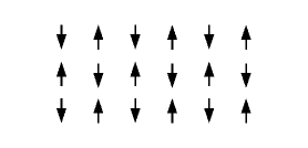
Figure 1: The ground state for the spin-1/2 antiferromagnetic Ising model on the square lattice.

In bipartite lattices we can divide the total system in two subsystems so that particles, belonging to the first subsystem, are nearest neighbors to particles, belonging to the other subsystem. If the interaction is between only nearest neighbors, pair antiferromagnetic bonds have minimal energies and the global optimal state of the system can be realized by minimizing coupling energies for each pair. However, there exist many lattices, which we cannot divide into two sublattices. For such systems we have a problem with the use of mean-field-like approximation or spin wave theory: The optimal state with the minimal energy is either not determined there, or there are many such states (too many, their number is of order of number of magnetic particles in the system), so that we cannot realize the knowledge of the ground state. The simple example is the triangular two-dimensional lattice. The elementary cell of the triangular lattice is a triangle.

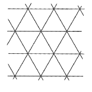
Figure 2: The example of non-bipartite two-dimensional lattice: triangular lattice.

Another example of such a lattice is the so-called Kagome lattice, known due to traditional Japanese bamboo baskets. It is composed of the arrangement of interlaced triangles, which are organized so that each point where two laths cross has four neighboring pattern of a tri-hexagonal tiling. The elementary cell of the Kagome lattice is the star of David.

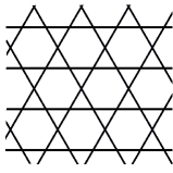
Figure 3: The example of non-bipartite two-dimensional lattice: Kagome lattice.

Notice that the crossing points of the Kagome lattice do not form a mathematical lattice, unlike the triangular lattice [17]. It has the symmetry p6m (or p3m1), like the triangular lattice. We can see that antiferromagnetic nearest-neighboring couplings cannot minimize the total energy of such a system. Hence, the standard approach, which brought so much success in studies of bipartite (antiferro)magnetic systems, fails for such lattices. Such magnetic systems are known nowadays as magnetically frustrated ones. In many magnetically frustrated systems magnetic ions do not develop long-range magnetic ordering for the reasons, which will be explained below. In that sense frustrated magnetic systems belong to the class of “spin-liquids” [18, 19]. The quantum spin liquid state is disordered, like in liquids, comparing to magnetically long-range ordered states. However, unlike other disordered states, a spin liquid state can be preserved down to very low temperatures (comparing to the values of spin-spin interactions). The interest to magnetically frustrated systems is caused not only by their interesting physical properties; such materials are perspective from the point of view of their use as data storage and memory, or as possible realization of topological quantum computation.

2 Frustration

We call the system as frustrated if it cannot minimize its total energy (the macroscopic state) by minimizing the interaction between each pair involved into the interaction, i.e., to perform such a minimization pair by pair [20, 21]. On the other hand, it is often used to call the system frustrated if its ground state is highly degenerate, and the level of degeneracy is of order of the number of particles in the system. Magnetic systems are the most known example of the manifestation of frustration.  However, naturally, the phenomenon of frustration is not limited to magnetic systems. For example, among frustrated systems we can count liquid and molecular crystals (like solid N₂), arrays of Josephson junctions, as well as the so-called “nuclear pasta state” of spatially modulated nuclear density inside stars (caused by the competition between Coulomb interactions and short-range nuclear couplings).

It is usual to distinguish between random and geometrical frustrations. Let us, first, discuss in short the former, because our review is mainly devoted to the latter. The random frustration, in turn, can be divided into dynamical and quenched one, by the origin. The characteristic feature of the dynamical (annealed) random frustration is related to multiple length scales, which are developed in time for spatially inhomogeneous systems with competing interactions. If such dynamical processes are frozen out, the randomness, and, in turn, frustration, is quenched. To remind, in statistical physics we usually call some parameters as quenched when they are random variables which do not evolve in time. Quenched frustration appears in systems, in which frozen degrees of freedom are not homogeneous, e.g., they cannot be periodically translated. Such a phenomenon can be observed in many metallic alloys with magnetic ingredients, which interact with each other via the long-range sign-changing Rudermann-Kittel-Kasuya-Yoshida (RKKY) coupling [9, 10, 11]. The main example of the manifestation of the random frustration in magnetic systems is a spin glass [22, 23, 24, 25, 26, 27], i.e., an ordered magnet with stochastic positions of spins with competing possible ferromagnetic and antiferromagnetic interactions between them, see the example in Fig. 4.

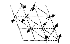
Figure 4: Illustration of a spin glass state: Spins are randomly distributed on a regular lattice.

The spontaneous magnetization of spin glasses is zero, however the magnetic ordering exists in the form of long-ranged spin-spin correlations.

In this review we will mostly deal with the geometric frustration. Here particles sit on the sites of regular lattices, unlike the situation with random frustration. However, local pair particle-particle interactions are in a conflict with each other: Each bond favors its own spatial correlation. Then it is impossible to satisfy all local interactions. The most known example is related to Ising spins 1/2 (which can be directed only up and down); they interact antiferromagnetically only with nearest neighbors on a two-dimensional equilateral triangular lattice. Clearly, antiferromagnetic bonds tend each neighboring spins to be antiparallel to each other, but it is impossible to realize, hence frustration. An example of the elementary cell of such a system is presented in Fig. 5.

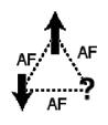
Figure 5: Elementary cell of the antiferromagnetic spin-1/2 Ising model on the two-dimensional equilateral triangular lattice. It is impossible to satisfy all three antiferromagnetic bonds simultaneously.

Geometrical frustration is possible not only if spins are collinear, but for spins arranged non-collinearly. Geometrically frustrated systems often manifest a residual entropy. The residual entropy, by definition, is the amount of entropy present even if the system is cooled arbitrary close to zero temperature. It exists for systems, in which many different microscopic states can persist when cooled to zero temperature, e.g., if the system has many different ground states with the same energy: degenerate ground states. Such a situation can also exist if such states have slightly different energies, but the system is prevented from settling in the “real” ground state with the lowest energy. The latter can be realized, e.g., if the system is very swiftly cooled. The most known example for systems possessing residual entropy is any amorphous system, like a glass. There the reason for residual entropy is caused in a great number of different ways of realization of microscopic structures in a macroscopic system. The interesting property of geometrically frustrated magnetic systems, like spin ice (see below) is that the level of residual entropy can be controlled by the application of an external magnetic field. This property of geometrically frustrated magnetic systems can be used for creation of refrigeration systems. In fact, geometrically frustrated magnetic systems had been studied earlier than the term “frustration” has been used [28, 29, 30]. For the review on frustrated spin systems, consult, e.g., the interesting books [31, 32]. Perhaps, it is worthwhile to discuss here the convenient measure of the level of frustration in geometrically or randomly frustrated magnetic systems. So-called frustration index $f$ has been proposed [33]. It is determined as $f=|\theta_{\rm CW}|/T_{c}$, where $\theta_{\rm CW}$ is the Curie-Weiss temperature, which can be extracted from the temperature behavior of the inverse magnetic susceptibility, and $T_{c}$ is the (critical) temperature at which the magnetic system possesses the long range order (say, the Néel temperature for antiferromagnets, or freezing temperature for spin glasses). Clearly, for magnetically disordered frustrated spin systems we would have $f\to\infty$. However, in the most of real magnetic systems spin-spin interactions (for example, magnetic dipole-dipole interactions, which are present in any magnetic system) should develop magnetic ordering, though at very low temperatures. Geometrically frustrated magnetic systems have been reviewed in [34, 35, 36, 37, 38, 39].

Probably, the oldest example of the geometrically frustrated system is the usual water ice.

3 Water Ice

It is well known that the molecule of water consists of two hydrogen atoms connected with the help of a covalent bond to the oxygen atom. Water ice is the frozen water, i.e., it is the water in the solid state. Depending on the external temperature and pressure water molecules in (water) ice can be organized in different forms. At ambient pressure the water ice can exist in three common forms: the ice I_h, or the hexagonal ice, which possesses the hexagonal symmetry, the most common phase of the water ice; the ice I_c, or the cubic ice, in which the cubic symmetry persists, and the ice XI with the orthorhombic symmetry (the space group Cmc2₁) [40]. The ice I_c or sphalerite, is the metastable phase existing, as a rule, between 130 K and 220 K, in which oxygen atoms organize a cubic diamond structure [41]. The ice XI is the proton (hydrogen)-ordered low-temperature (below 72 K) form of the hexagonal ice. It contains eight water molecules per unit cell. The internal energy of the ice XI is about 0.17 times lower than the one for the hexagonal ice I_h. It is a ferroelectric, see, e.g., [42].

The hexagonal ice, also known as ice one, or wurzite, is the water ice, which properties permitted to give the name to spin ices. It is stable down to approximately 73 K. Its symmetry is hexagonal with nearly tetrahedral bonding angles ($\arccos(-1/3)\approx 109.5^{\rm o}$) of the crystal structure. The latter consists of crinkled (alternating in the ABAB pattern) planes composed of tessellating hexagonal rings (a repetition of rings without gaps and overlaps, like in Escher’s pictures). B planes are reflections of A planes along the same axes as the planes themselves. Oxygen sits in each vertex, and edges of rings are formed by hydrogen bonds [43, 44].

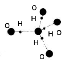
Figure 6: Configuration of oxygens and hydrogens in the hexagonal water ice (oxygen: large spheres, hydrogen: small spheres). Each oxygen-oxygen bond has two steady-state positions of hydrogen. The configuration satisfies Bernal-Fowler ice rules: One hydrogen per oxygen-oxygen bond, and each oxygen neighbors two close hydrogens and two sitting far hydrogens.

Two molecules of water can form a hydrogen bond between them. In a liquid water more bonds are possible because oxygen of a single water molecule has two lone pairs of electrons, each can form a hydrogen bond with another molecule with the angle between hydrogen atoms 104.45^o and with the distance from hydrogen to oxygen being 95.84 pm. The side with oxygen atom in the water molecule has a partial negative charge due to higher electronegativity of the oxygen comparing to hydrogen. It means that the hydrogen side is partially positive, i.e., the water molecule is a dipole. The charge difference yields attraction between water molecules, which contributes to the hydrogen bonding. Every water molecule has hydrogen bonds with up to four other water molecules, because it can accept two and donate two hydrogens, see Fig. 6. The hydrogen bonding energy of the water molecule is relatively strong (it is weak, though, comparing to covalent bonds within the water molecule). Hydrogen bonds with almost tetrahedral bonding angles of the water molecule, cf. Fig. 6, help to organize an open hexagonal lattice of the hexagonal ice. The distance between oxygen atoms along each bond is about 275 pm, which is much larger than the distance between oxygen and hydrogen in the water molecule. Large hexagonal rings leave almost enough room for another water molecule to exist inside, which yields the density of ice being lower than of the water.

Hydrogen atoms (in fact, almost protons) sit very close along hydrogen bonds in the crystal lattice of the hexagonal ice (Fig. 6), i.e., each water molecule is preserved there. It implies that in the hexagonal ice each oxygen has two adjacent hydrogens at about 101 pm (along the 275 pm hydrogen bond), i.e., not in the middle of the distance between two oxygens. Basically, two equivalent hydrogen positions exist in each oxygen-oxygen bond. Four-fold oxygen coordination yields one hydrogen per such a bond. In the structure of the hexagonal water ice that way is determined by the Bernal-Fowler ice rules [45]. The first one is related to one hydrogen per oxygen-oxygen bond in average in the ice crystal. The second ice rule states that for each oxygen two hydrogens have to be close, and two protons sit far from the oxygen. It turns out that the second ice rule frustrates the low-energy problem of the water ice caused by the stability of water molecules in it. As a result, the crystal structure contains the residual (zero temperature) entropy inherent to the lattice. In other words, the hexagonal ice is expected to have the intrinsic randomness even if it was possible to cool it to zero temperature. In ideal situation the hexagonal (water) ice can never be completely frozen, seemingly violating the third law of thermodynamics! Such an entropy in the hexagonal water ice is defined by the number of possible configurations of hydrogen positions which can be formed (the requirement of two hydrogens to be related to each oxygen in the closest proximity with each hydrogen bond, which join two oxygen atoms having only one hydrogen, holds). The residual entropy of the hexagonal ice is ${\cal S}_{0}\approx 3.5$ J mol^-1 K^-1. That value has been measured in the set of experiments devoted to the investigation of the specific heat of the hexagonal water ice [46, 47].

The structure of the hexagonal ice has been pioneered by Linus Pauling [the only person who was awarded by two unshared Nobel Prizes: Chemistry (1954) and Peace (1962) prizes] in 1935 [48]. He has noticed that the number of configurations with two hydrogen being close to the oxygen, and two hydrogens being far from it grows exponentially with the system size. It implies the extensive character of the residual entropy of the hexagonal water ice. Pauling has estimated the value of the residual entropy in the hexagonal water ice. One mole of ice contain $N$ oxygens, and therefore $2N$ oxygen-oxygen bonds. Each such a bond can have two possible positions for a hydrogen, which implies $2^{2N}$ possible hydrogen positions for the total crystal. Only six configurations are energetically favorable out of 16 possible ones for each oxygen. The upper limit for a number of ground state configurations, $M$, can be, therefore, estimated as $2^{N}(6/16)^{N}=(3/2)^{N}$. Corresponding entropy can be calculated as ${\cal S}_{0}=Nk_{\rm B}\ln(3/2)$, which gives 3.37 J mol^-1 K${}^{-1}\approx 0.323k_{\rm B}$. That value agrees very well with the experimentally measured [46, 47]. Despite calculations performed by Pauling missed the global constraint of the number of hydrogens and local constraints caused by closed loops in the lattice of the hexagonal water ice, its accuracy is of order of 1-2 % [49]. It has been calculated numerically for the two- and three-dimensional ice model (see below).

3.1 Ice Models

Ice-type models, i.e., the ones, which possess ice rules, are often studied in statistical mechanics: They are the particular case of vortex models, namely, the six-vortex models. Any ice model is defined on a lattice with the coordination number 4, i.e., each vertex is connected to four nearest neighbors by an edge. Each bond is represented by an arrow, so that the number of arrows pointing to the vortex is two (as well as the number of arrows pointing outwards), which constitutes the ice rule in the vertex model. So far, mostly two- and three-dimensional ice vertex models has been studied. For instance, for the square ice model six configurations are valid. The energy of the state $E$ is given by $E=\sum_{i=1}^{6}\varepsilon_{i}n_{i}$, where $n_{i}$ is the number of vertices with $i$-th configuration (of six possibilities), and $\varepsilon_{i}$ being the energy associated with the vertex configuration $i$. Fig. 7 shows six possible configurations of the six-vertex square model, which satisfy the ice rule.

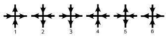
Figure 7: Six possible configurations of the square ice model, possessing ice rules: In each vertex two arrows point inwards and two arrows point outwards.

The six-vertex model on a square lattice can model a ferroelectric [50], where $\varepsilon_{1,2,3,4}>0$ and $\varepsilon_{5,6}=0$. If there is no external field, the condition $\varepsilon_{1}=\varepsilon_{2}$, $\varepsilon_{3}=\varepsilon_{4}$ and $\varepsilon_{5}=\varepsilon_{6}$ holds. The six-vertex model on a square lattice has been exactly solved by E. Lieb [51, 52, 53]. He has found the residual entropy there ${\cal S}_{0}=(3/2)Nk_{\rm B}\ln(4/3)$, and the value $(4/3)^{3/2}\approx 1.5396$ is known as the Lieb’s square ice constant. Later Lieb’s solution has been generalized for the cases with [54] and without external field [55]. Naturally, one can consider more realistic models, than the two-dimensional six-vertex model on the square lattice. However, for the three-dimensional ice-type model the exact solution has been obtained [56] only for the special temperature interval, where the model is called to be “frozen”, which means that in the thermodynamic limit the energy and entropy per vortex are zero in such a range of $T$. Ice-type vertex models in statistical mechanics are generalized for the eight-vertex model, which also possesses exact solution [57].

4 Spinels: Cation ordering and antiferomagnetic models

The similarity of the water ice problem to the ordering of cations in the so-called inverse spinel material has been pointed out by E.J.W. Verwey [58, 59], and then has been discussed in detail by P.W. Anderson [60]. Spinels (called due to the natural mineral spinel MgAl₂O₄) are the class of materials with the general chemical formula AB₂O₄ with the cubic crystal system. A and B cations occupy octahedral and tetrahedral sites of the lattice, and can be divalent, trivalent or quadrivalent. In inverse spinels two kinds of cations on the B-sites of the spinel lattice are situated so that the total numbers of cations of each kind are equal. The B-sites of the spinel lattice form the so-called pyrochlore lattice. The latter [called due to pyrochlore, the natural mineral with the chemical formula (Na,Ca)₂Nb₂O₆(OH,F)] has Fd${\bar{3}}$m space group, often is related to systems with the chemical formulas A₂B₂O₆ or A₂B₂O₇. The pyrochlore lattice is organized of corner-sharing tetrahedra, which are alternating “upward” and “downward”, see Fig. 8.

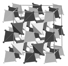
Figure 8: A- (light tetrahedra) and B-cites (dark tetrahedra) of A₂B₂O₇ in the vertices of corner-sharing tetrahedra form the pyrochlore lattice. From J.S. Gardner et al., Physical Review B 70, 180404(R) (2004). http://link.aps.org/abstract/PRB/v70/p180404 Copyright 2004 by the American Physical Society.

The minimum energy is related to the case, in which the number of pairs consisting of two different kinds of cations is maximal. Such a condition is satisfied if each elementary tetrahedron of the B-lattice of the inverse spinel material has two cations of one kind and two cations of the other kind, so called tetrahedron rule, analogous to the ice rule for the hexagonal water ice. Notice that in the spinel lattice centers of tetrahedra are situated on the same lattice as oxygens in the cubic I_c water ice. It implies that cation ordering in this problem could have residual entropy, like in the Pauling water ice.

Among spinels with different cations at B-sites we can distinguish the situation, in which the valency of ions is different from integer, like in the first non-rare-earth based heavy-fermion system LiV₂O₄ see, e.g., [61, 62, 63, 64, 65, 66, 67, 68, 69, 70], or in, probably, the oldest known magnetic material, magnetite, Fe₃O₄ see, e.g., [1, 58, 59]. There the formal valence of V ion is 3.5, and the one of Fe on B sites is 2.5 (the valence of Fe ions on A sites is 3), i.e., they have to exist in equal combinations of V³⁺ and V⁴⁺, or Fe²⁺ and Fe³⁺. Notice, however, that recent studies contradict the direct application of the ice (tetrahedron) rule to LiV₂O₄ and Fe₃O₄ [61, 62, 63, 64, 65, 66, 67, 68, 69, 70, 71, 72, 73, 74, 75]. For the recent reviews on spinel materials consult, e.g., [76, 77, 78, 79].

Similar situation appears if we consider the spin Ising antiferromagnetic model on the pyrochlore lattice. Here spin up and spin down correspond to two kinds of cations in the above mentioned spinel situation, or to “close hydrogen” or “far hydrogen”for the water ice. However, there is no realization of such an Ising model on the pyrochlore lattice. Why is it so? The pyrochlore lattice has the cubic symmetry. Hence, there is no reason for the unique direction of Ising spins in such a system. On the other hand, the situation with antiferromagnetic Heisenberg spins on a pyrochlore lattice is realistic. It was J. Villain, who pointed out that the classical Heisenberg antiferromagnet cannot be magnetically ordered on the pyrochlore lattice [80] due to the geometrical frustration down to zero temperatures. He called such system as a collective paramagnet to stress the absence of ordering, on the one hand, and collective nature of magnetic properties, on the other hand.

5 Spin ice

Magnetic systems, in which magnetic ions reside on lattices of corner-sharing tetrahedra (pyrochlore lattice), belong to the most known examples of magnetic systems with geometrical frustration. Among them, maybe the most interesting properties are revealed by the cubic pyrochlore oxides of the family A₂B₂O₇ with magnetic A ions and nonmagnetic B ones [81, 82, 83, 84]. Such systems can be metallic, or insulating. The space group for that systems is Fd${\bar{3}}$m. It is usual to use another chemical formula, namely A₂B₂O₆O’ to emphasize the difference in positions of oxygen ions. Here A ion is placed in 16d position in the Wyckoff classification [minimal coordinates are (1/2,1/2,1/2)], B ion is in 16c placed at the origin [i.e., minimal coordinates are (000)], O is in 48f (x,1/8,1/8) and O’ is in 8b (3/8,3/8,3/8). Here the parameter x is of range 0.32-0.345. All six B-O bonds have equal lengths, and O-B-O angles have almost ideal octahedral values of 90^o, i.e., oxygens surround B-ion at vertices of the perfect octahedron. As for A-ion, oxygen ions form the perfect cube, but with strong distortions. In fact, the surrounding of the A-site can be considered as six-membered ring of O with two O’ atoms, which form a stick, oriented perpendicular to the ring, see Fig. 9.

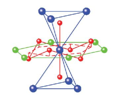
Figure 9: (Color online) The environment of the A-site of pyrochlore oxides. Large (blue) spheres denote rare-earth ions, medium (green) spheres denote nonmagnetic metal ions, and small (red) spheres are oxygens. Six oxygens (O) lie in plane, and two (O’) are situated on the line, perpendicular to basal plane. From A. Yaouanc et. al., Physical Review B 84, 172408 (2011). http://link.aps.org/abstract/PRB/v84/p172408 Copyright 2011 by the American Physical Society.

This is why, A-ions have a large axial symmetry, with the axes parallel to [111] directions (diagonals of the cube). Basically, such a axial symmetry produces a large crystalline electric field at A site, which is the origin of the Ising-like properties of magnetic ions situated at the A position.

Probably, the most interesting representatives of pyrochlore oxides are the ones with A being trivalent rare-earth ions, like Gd, Tb, Dy, Ho, Yb, etc., or Y, and with a tetravalent ion in B-position, as Ti, Sn, Mo, Mn, etc. Both A and B ions can be magnetic or non-magnetic.

We will concentrate now on insulating titanates of Dy and Ho [85] (Dy₂Ti₂O₇, and Ho₂Ti₂O₇), and on similar compounds, stannates, with the replacement of non-magnetic Ti⁴⁺ by the non-magnetic Sn⁴⁺. In this case only A-sublattice (which is the FCC lattice of corner-sharing tetrahedra, directed up and down) is responsible for magnetic properties. The primitive basic cell has four rare-earth ions sitting at the vertices of each tetrahedron. However, the conventional cubic unit cell of pyrochlore oxides has the size $a\sim 10$ Åwith 16 rare-earth ions, i.e., it consists of four primitive tetrahedron cells directed “up” and “down”. The distance between nearest neighboring rare-earth ions is $x=\sqrt{2}a/4\sim 3.5$ Å.

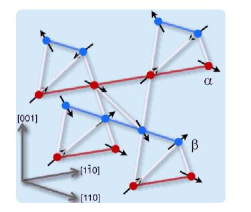
Figure 10: (Color online) $\alpha$ and $\beta$ chains in the pyrochlore lattice. From J.P. Clancy et al., Physical Review B 79, 014408 (2009). http://link.aps.org/abstract/PRB/v79/p014408 Copyright 2009 by the American Physical Society.

It is also interesting to notice that the pyrochlore lattice for A sites can be considered as two sets of orthogonal chains, the one being parallel to [110] direction (called $\alpha$ chains) and the other one parallel to [1${\bar{1}}$0] direction (refereed to $\beta$ chains, see Fig. 10).

5.1 Single ion properties

Dy (Ho) ions have [Xe]6S²4f⁹ (4f¹⁰) ground state electron configuration. Rare-earth ions due to strong spin-orbit coupling form the total moment ${\bf J}={\bf L}+{\bf S}$, where ${\bf L}$ (${\bf S}$) is the total orbital (spin) moment. According to Hund’s rules, we can find $J=15/2$ for Dy³⁺ ion with $L=3$ and $S=9/2$, and $J=8$ with $L=3$ and $S=5$ for Ho³⁺. The $(2J+1)$ degeneracy of the configuration is lifted due to the crystalline electric field of ligands (oxygens). The crystal field Hamiltonian can be written for ${\bar{3}}$m ($D_{3d}$) point symmetry of the A site as [86, 87, 88, 89, 90]

$${\cal H}_{\rm cf}=\sqrt{4\pi}\sum_{l,m}{B_{l}^{m}Y_{l}^{m}\over\sqrt{2l+1}}=\sum_{l,m}B_{l}^{m}{\cal O}_{l}^{m}$$

$$=B_{2}^{0}{\cal O}_{2}^{0}+B_{4}^{0}{\cal O}_{4}^{0}+B_{4}^{3}{\cal O}_{4}^{3}$$

$$+B_{6}^{0}{\cal O}_{6}^{0}+B_{6}^{3}{\cal O}_{6}^{3}+B_{6}^{6}{\cal O}_{6}^{6}\ ,$$ (1)

where $B_{l}^{m}$ are crystal field coefficients, $Y_{l}^{m}$ are spherical harmonics, and ${\cal O}_{l}^{m}$ are Stevens operators [6, 91], related to the projections of the total moment. For $L=3$ we limit ourselves with $l\leq 6$, due to the Wigner-Eckart theorem. Further restriction comes about because the crystalline electric field environment is symmetric under operations of the point group $D_{3d}$. Here we use [6, 91, 92, 93] ${\cal O}_{2}^{0}=3J_{z}^{2}-j(J+1)$, ${\cal O}_{4}^{0}=35J_{z}^{4}-[30J(J+1)-25]J_{z}^{2}+3J^{2}(J+1)^{2}-6J(J+1)$, ${\cal O}_{4}^{3}=(1/4)[3(J_{+}^{3}-J_{-}^{3})+2(J_{+}^{3}+J_{-}^{3})J_{z}]$, where $J_{\pm}=J_{x}\pm iJ_{y}$, ${\cal O}_{6}^{0}=231J_{z}^{6}-[315J(J+1)-735]J_{z}^{4}+[105J^{2}(J+1)^{2}-525J(J+1)+294)J_{z}^{2}-5J^{3}(J+1)^{3}+40J^{2}(J+1)^{2}-60J(J+1)$, ${\cal O}_{6}^{6}=(1/2)(J_{+}^{6}+J_{-}^{6})$, and ${\cal O}_{6}^{3}=(1/4)[3(40-3J(J+1))(J_{+}^{3}-J_{-}^{3})+(179-6J(J+1))(J_{+}^{3}+J_{-}^{3})J_{z}+99(J_{+}^{3}-J_{-}^{3})J_{z}^{2}+22(J_{+}^{3}-J_{-}^{3})J_{z}^{3}]$. From the experiments on inelastic neutron scattering [86, 87, 88, 89, 90] we can find that for Ho₂Ti₂o₇ (Dy₂Ti₂o₇) the ground state can be described as the Kramers doublet with $|J=8,m_{J}=\pm 8\rangle$ ($|J=15/2,m_{J}=\pm 15/2\rangle$) with negligible contributions from components with other values of $m_{J}$ [higher multiplets are divided by the gap of order of $\Delta\sim 300$ K from the ground state Kramers doublet (in fact, the gap was estimated from 140 K to 380 K [86, 87, 88, 89, 90])]. This is why, at low temperatures we can consider Ho₂Ti₂o₇ and Dy₂Ti₂o₇ as systems of effective Ising spins 1/2. However, the situation is different from the case of a standard uniaxial anisotropy, because most often the “easy axis” is homogeneous for magnetic systems [3, 4, 5], and in the considered case we have four equivalent “easy axes” for each tetrahedron parallel to [111] directions, see Fig. 11.

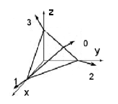
Figure 11: Elementary cell for the A-site pyrochlore oxide lattice. Vectors labeled 0,1,2,3 are unit vectors directed along [111] axes, which are distinguished by the magnetic “easy-axis” anisotropy.

We can introduce unit vectors directed along the “easy axes” ${\bf e}_{0,1}=({\bf x}\pm{\bf y}\pm{\bf z})/\sqrt{3}$, ${\bf e}_{2,3}=(-{\bf x}\pm{\bf y}\mp{\bf z})/\sqrt{3}$, where ${\bf x}$, ${\bf y}$ and ${\bf z}$ are the unit vectors along the co-ordinate axes. Then at low temperatures $T\ll\Delta$ we can approximate

$${\bf J}_{n}\to|\langle J_{z}\rangle|\sigma_{n}^{z}{\bf e}_{n}\ ,$$ (2)

where $\sigma^{z}_{n}$ are Pauli matrices, which have eigenvalues $\pm 1$, $|\langle J_{z}\rangle|\approx 15/2$ for Dy₂Ti₂O₇ and $|\langle J_{z}\rangle|\approx 8$ for Ho₂Ti₂O₇. There are no other components $\sigma_{n}^{x,y}$ in the low-temperature approximation, and, therefore, the low-energy physics can be approximated by the Ising model. Sometimes this situation is called classical, to stress that there is no spreading of excitations in the Ising model, and variables commute with each other. However, it can be misleading, because the Ising system has a discrete spectrum, the hallmark of quantum physics.

The external magnetic field ${\bf B}$ at low temperatures acts as

$${\cal H}_{Z}=-g\mu_{B}\sum_{n}({\bf B}\cdot{\bf J}_{n})$$

$$\approx-g\mu_{B}|\langle J_{z}\rangle|\sum_{n}({\bf B}\cdot{\bf e}_{n})\sigma^{z}_{n}\ ,$$ (3)

where $\mu_{B}$ is Bohr’s magneton, equal to 9.27$\times 10^{-24}$ J/T, or, more convenient for us, 0.671 K/T, if we measure all energies in Kelvins, and $g$ is the Landé $g$-factor, equal to 4/3 for Dy³⁺ and 5/4 for Ho³⁺. Then the characteristic energy scale for the Zeeman interaction of pyrochlore oxides is $10\mu_{B}|B|\sim 6.71|B|$ K, where the magnitude of the magnetic field $|B|$ is measured in Tesla. Obviously, for the values of the field $|B|\leq 45$ T such an energy is lower than $\Delta\sim 300$ K, and the Ising approximation is justified. For higher values of the field we have to take into account higher-energy multiplets due to crystalline electric field.

We can also neglect the van Vleck contribution to the magnetic susceptibility of the considered pyrochlore oxides, and the contributions from the high-energy multiplets, caused by the crystalline electric field, to the susceptibility at low temperatures.

5.2 Realization of the ice rule

Now we are in position to explain why these pyrochlore oxides are known as spin ices. Namely, let us consider the Hamiltonian of exchange interactions between rare-earth magnetic ions ${\cal H}_{ex}=-(1/2)\sum_{i,j}{\cal J}_{i,j}({\bf J}_{i}\cdot{\bf J}_{j})$, where $i$ and $j$ denote positions of magnetic ions, and ${\cal J}_{i,j}$ are the exchange integrals. The prefactor (1/2) is introduced to avoid double counting of sites. Here we limit ourselves with the isotropic version of the exchange coupling. Notice, however, that the symmetry allows four distinct types of anisotropic exchange interactions in a pyrochlore lattice [94, 95]. For rare-earth systems 4f orbitals are screened by 5s and 6p orbitals, and, therefore, the exchange interaction (both, the direct exchange between rare-earth ions themselves, and the indirect exchange via oxygen ions O^2-) is expected to be small. Then at low temperatures we can approximate that expression as

$${\cal H}_{ex}\approx-|\langle J_{z}\rangle|^{2}\sum_{i,j}{\cal J}_{i,j}({\bf e}_{i}\cdot{\bf e}_{j})\sigma_{i}^{z}\sigma_{j}^{z}\ .$$ (4)

The value of the exchange integrals for nearest neighboring Dy³⁺ in Dy₂Ti₂O₇ has been estimated [96, 97] as ${\cal J}_{ij}\sim 0.66$ mK. We can introduce $J\equiv|\langle J_{z}\rangle|^{2}{\cal J}_{i,j}$. For Ho-based titanate its value is estimated as $J\sim 4.22$ K, and for Dy-based titanate it is $J\sim 3.71$ K, i.e., in both cases $J\ll\Delta$. Notice that $J>0$, i.e. it corresponds to the ferromagnetic nearest neighbor coupling in the initial exchange Hamiltonian. For nearest neighbors we can write cf. [98]

$${\cal H}_{ex}\approx-J\sum_{\langle i,j\rangle}({\bf e}_{i}\cdot{\bf e}_{j})\sigma^{z}_{i}\sigma^{z}_{j}=(J/3)\sum_{\langle i,j\rangle}\sigma^{z}_{i}\sigma^{z}_{j}\ ,$$ (5)

where we limit ourselves with the nearest neighbors $\langle i,j\rangle$, and used the equality $({\bf e}_{i}\cdot{\bf e}_{j})=-1/3$ for the tetrahedron, which follows from the definition of the unite vectors ${\bf e}_{n}$. Using the definition $S_{t}=(\sigma^{z}_{0}+\sigma^{z}_{1}+\sigma^{z}_{2}+\sigma_{z}^{3})_{t}$ as the total effective Ising spin for the tetrahedron, we can get [99]

$${\cal H}_{ex}\approx{J\over 6}\sum_{t}S_{t}^{2}-{2N_{t}J\over 3}\ ,$$ (6)

where the summation is over each tetrahedron primitive cells, $N_{t}$ is the total number of such cells. It is important to emphasize that the ferromagnetic exchange between real total moments in such pyrochlore oxides produces the effective antiferromagnetic coupling between effective Ising spins. Then, it is clear from Eq. (6) that for $J>0$ the lowest energy has the state with $S_{t}=0$. It is equivalent to the ice rule in the water ice, or to the Verwey’s tetrahedron rule: The lowest energy is related to states of each tetrahedron with to Ising spins directed inside, and two others directed outside the tetrahedron which means two of $\sigma^{z}_{n}$ have +1 eigenvalue, and two others have -1 eigenvalue (notice that all spins have directions parallel to [111] axes, cf. Fig. 12). The fulfillment of the ice rule implies the frustration, totally equivalent to the water ice I_h. That suggested the name for such systems: Spin ices! It is interesting to remark that the antiferromagnetic exchange between total moments has to manifest the non-frustrated state with all effective Ising spins having the same signs of their eigenvalues. In other words, the real antiferromagnetic exchange produces the ground state with all effective Ising spins directed either in or outside each tetrahedron.

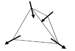
Figure 12: Realization of the ice rule in the primitive cell of a spin ice.

At low temperatures additional spin-spin interaction may manifest itself, the magnetic dipole-dipole interaction, which Hamiltonian is (the importance of the magnetic dipole-dipole interactions for spin ices has been pointed out, e.g., in [100])

$${\cal H}_{d}=\left[{\mu_{0}\over 4\pi}\right]{g^{2}\mu^{2}_{\rm B}\over 2x^{3}}\sum_{i,j}\biggl{[}{({\bf J}_{i}\cdot{\bf J}_{j})\over(|{\bf r}_{ij}|^{3}/x^{3})}$$

$$-{3({\bf r}_{ij}\cdot{\bf J}_{i})({\bf r}_{ij}\cdot{\bf J}_{j})\over(|{\bf r}_{ij}|^{5}/x^{3})}\biggr{]}$$

$$\approx\left[{\mu_{0}\over 4\pi}\right]{g^{2}\mu^{2}_{\rm B}|\langle J_{z}\rangle|^{2}\over 2x^{3}}\sum_{i,j}\sigma_{i}^{z}\sigma_{j}^{z}{({\bf e}_{i}\cdot{\bf e}_{j})\over(|{\bf r}_{ij}|^{3}/x^{3})}$$

$$-{3({\bf r}_{ij}\cdot{\bf e}_{i})({\bf r}_{ij}\cdot{\bf e}_{j})\over(|{\bf r}_{ij}|^{5}/x^{3})}$$ (7)

where ${\bf r}_{ij}={\bf r}_{i}-{\bf r}_{j}$, and $\mu_{0}/4\pi=10^{-7}$ N A ^-2 ($\mu_{0}$ is the vacuum permeability), and for convenience we have normalized every contribution to the value for the nearest neighbors. Then the magnetic dipole-dipole contribution to the nearest neighbor interaction between effective Ising spins in the primitive cell is $D=\mu_{0}g^{2}\mu^{2}_{\rm B}|\langle J_{z}\rangle|^{2}/8\pi x^{3}$. We can estimate this value as 1.4 K. Hence, the nearest neighbor part of the magnetic dipole-dipole interaction renormalizes the exchange interaction [96, 101], and the conclusions made above using the only exchange coupling seem to hold for the nearest neighbor dipole-dipole interactions. However, it is not the total story. Unlike exchange couplings, magnetic dipole-dipole interactions are long-ranged (the model, which take into account long-ranged dipole-dipole coupling is called the dipole spin ice). This has been taken into account in several ways. First, some truncation for the dipole-dipole interaction was used [96, 102]. Then Ewald summation [103], usually used for the estimation of the long-range dipole-dipole coupling [104], Monte-Carlo simulations [104, 105, 106, 107], and mean-field calculations [108, 109, 110] were also performed. They found that the long-range part of the magnetic dipole-dipole interaction can produce the long-range Néel-like ordering (via the first order phase transition) at very low temperatures. Hence, the dipolar spin ice is characterized by ordering with the commensurate propagation wave vector of the order parameter, and, therefore, the long-range dipole-dipole coupling removes the degeneracy, caused by the frustration. From this perspective, spin ices are equivalent to the water ice, which manifests the transition from the frustrated hexagonal and cubic phases to the orthorhombic ice XI phase. Such a phase transition in spin ices has not been observed yet see, e.g., [111]. From the theoretical viewpoint, it was unclear why the ice rule is satisfied in dipolar spin ices. The reason has been clarified in [112]. The autors of [112] have pointed out that the tetrahedron (ice) rule $S_{t}=0$, or more general, $\sum_{i}S_{t,i}=0$, where the sum is performed over all tetrahedra, is equivalent to some “spin field” ${\bf B}_{s}({\bf r})$, which divergence is zero, $(\nabla\cdot{\bf B}_{s})=0$ (notice that we deal with the lattice case). Nonzero flux of that field means broken tetrahedron (ice) rule. Then the correlation functions for the field are

$$\langle B_{\alpha}({\bf r})B_{\beta}(0)\rangle\sim{3x_{\alpha}x_{\beta}-r^{2}\delta_{\alpha,\beta}\over r^{5}}\ ,$$ (8)

where $\alpha,\beta=x,y,z$. The dipolar Hamiltonian on the pyrochlore lattice can be presented as the projector, and the correlations of the projector are equivalent to the projector itself [112]. That means that the local constraint, i.e., the tetrahedron rules, yield dipolar-like correlations at large distances. these Coulomb correlations are the signature of the so-called  Coulomb phase” in dipole spin ices, see, e.g. [113, 110, 114, 115].

5.3 Experimental discovery of spin ices

In fact, spin ices were discovered experimentally in [116, 117, 118, 119]. The authors of [116] (who, actually, first used the term spin ice) performed the neutron scattering experiment to investigate low (down to 0.05 K) temperatures properties of Ho₂Ti₂O₇. At zero magnetic field they have observed no magnetic ordering by the neutron scattering (down to 0.35 K) and by muon spin rotation (down to 0.05 K). They have found positive $\theta_{\rm CW}\approx 1.9$ K, indicating ferromagnetic interactions. It is interesting that $\theta_{\rm CW}$ is of the same order of values as both $D$ and $J$. naturally, the absence of $T_{c}$ (or, similar, $T_{c}\ll\theta_{\rm CW}$) implies very high level of frustration in this compound. The magnetic field affected the neutron scattering depending on the pre-history of the sample (see also [120, 121, 122]). It is similar to the situation in spin glasses [22, 23, 24, 25, 26, 27, 123], despite absent (or very weak) randomness in Ho₂Ti₂O₇. Such experiments have been tried to be explained [124] by considering the ferromagnetic Ising spins directed along [111] in the pyrochlore lattice.

Even more important for the analogy between the hexagonal water ice and the spin was the measurement of the specific heat $c(T)$ in Ref. [119] in Dy₂Ti₂O₇. The authors of [119] followed the strategy of Ref. [46, 47] to get the value of the residual entropy in spin ice material, similar to what had been performed for the water ice. The entropy for the water ice has been calculated by integration of $c(T)/T$ starting from 10 K till the gas phase,

$$\Delta{\cal S}_{1,2}={\cal S}(T_{1})-{\cal S}(T_{2})=\int_{T_{1}}^{T_{2}}{c(T)dT\over T}\ ,$$ (9)

with an addition of the latent heat at the melting and vaporization. Then, calculated in such a way value has been compared with the expected from calculations (see above) absolute value for the hexagonal water ice. In Ref. [119] it has been measured the magnetic specific heat of Dy₂Ti₂O₇ between the temperatures $T_{1}=0.3$ K and $T_{2}=10$ K. The former, according to estimations, is related to the spin ice phase (its value was lower than the temperature of the maximum in the dependence $c(T)$ at 1.24 K, identified as the crossover temperature [119]), while the latter expected to be already in the paramagnetic regime, where one can neglect spin-spin interactions. The Schottky-like maximum in $c(T)$ was connected to the energy gap between the states satisfying the ice rule (two spins directed “in” the tetrahedron, and two “out”) and the excited state with one spin “in” and three spins directed “out” (or vice versa). In the low temperature regime, $T<1.24$ K, the spin flip rate has been calculated to be exponentially decaying [104], because of the steady-state settling to the ice rule “phase”. The restored that way value of the magnetic entropy in the limit $T\to T_{2}$ was obtained as 3.9 J mol^-1K^-1, which is very close to the difference between the magnetic entropy in the paramagnetic regime (free effective Ising spins), $k_{\rm B}N_{\rm A}\ln(2)=5.76$ J mol^-1K^-1 (here $N_{\rm A}$ is the Avogadro number), and the Pauling value $k_{\rm B}N_{\rm A}\ln\sqrt{3/2}=1.68$ J mol^-1K^-1. The results of later experiments [125, 126, 127] have shown even better agreement between the measured value of the entropy and the one, predicted by Pauling, see Fig. 13. Moreover, by studying Dy_2-xY_xTi₂O₇, i.e., by replacing the magnetic Dy³⁺ ion by the non-magnetic Y³⁺, [127] has proven that the considered entropy is related namely to magnetic subsystem of spin ices. Performed Monte-Carlo simulations [96] show a very good agreement with the observed temperature behavior of the specific heat and entropy in Dy₂Ti₂O₇.

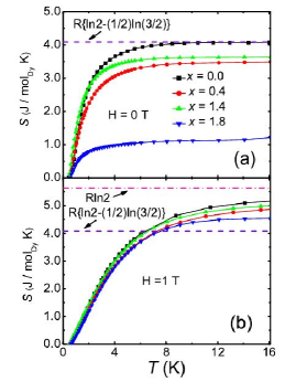
Figure 13: (Color online) Entropy of Dy_2-xY_xTi₂O₇ as a function of temperature without (upper panel) and with the external magnetic field. We can see that the entropy is related to magnetic ions Dy³⁺, because higher concentration of Y³⁺ ions decreases the value of ${\cal S}$ in the system. From X. Ke et al., Physical Review Letters 99, 137203 (2007). http://link.aps.org/abstract/PRL/v99/p137203 Copyright 2007 by the American Physical Society.

On the other hand, Ho₂Ti₂O₇ does not show such a direct evidence of the low temperature specific heat and entropy, as Dy₂Ti₂O₇. The reason for such a difference in the behaviors of two representatives of the spin ice group is connected with the anomalously large hyperfine interaction between nuclear and electron spins, characteristic for Ho³⁺. Such an interaction manifests itself in a Schottky anomaly in the temperature dependence of the magnetic specific heat of Ho₂Ti₂O₇ at about 0.3 K. If one subtracts the nuclear contribution, the residual Pauling entropy in Ho₂Ti₂O$7$ can be manifested [128, 101]. Similar observations [121, 129, 130, 131] were made for stannates Ho₂Sn₂O₇ and Dy₂Sn₂O₇.

Magnetic Coulomb phase in spin ices has been observed in [115] via the polarized neutron scattering.

5.4 Spin ices in an external magnetic field

First magnetic measurements in Dy₂Ti₂O₇ have been performed in [132, 133], in which the dc magnetic susceptibility and magnetic moment have shown a strong magnetic (Ising) anisotropy along [111].

The temperature and magnetic field dependencies of thermodynamic characteristics of spin ice systems can be calculated in the simplest way, e.g., by performing recently developed approach [134], in which the Bethe-Peierls approximation on a Bethe lattice was used. It assumes that effective fields acting on effective Ising spins of the primitive cell, Fig. 11, are the same as the ones, acting on cell’s nearest neighbors, which does not, actually, hold in pyrochlore system. However, results, obtained in this approximation, show a good qualitative agreement with the experimentally observed data, see below. In the Bethe-Peierls approach the free energy of the spin-ice system per rare-earth ion can be written as

$$F={k_{\rm B}T\over 4}\sum_{n=0}^{3}\ln[2\cosh(2f_{n}-b_{n})]$$

$$-{k_{\rm B}T\over 2}\ln[2Z({\bf f})]\ ,$$ (10)

where

$$Z({\bf f})=\sum_{m=0}^{2}Z_{m}({\bf f})e^{-2m^{2}J/k_{\rm B}T}.$$ (11)

The index $n$ denotes four directions (cf. Fig. 11) for the “easy axes” of the magnetic anisotropy (considered here to be much larger than the effective interactions between effective Ising spins) in each tetrahedron in the spin-ice system, see above, $b_{n}\equiv g\mu_{\rm B}|\langle J_{z}\rangle|({\bf e}_{n}\cdot{\bf B})/k_{\rm B}T$ are the projections of the external magnetic field ${\bf B}$ normalized by the temperature, and $f_{n}$ are the projections of the effective magnetic field, which acts on the effective Ising spins in the considered tetrahedron from other effective Ising spins in the system. In Eq. (11) $J$ denotes the value of the effective exchange interaction between spins in each tetrahedron, and

$$Z_{0}({\bf f})=\cosh(f_{0}+f_{1}-f_{3}-f_{3})$$

$$+2\cosh(f_{0}-f_{1})\cosh(f_{2}-f_{3})\ ,$$

$$Z_{1}({\bf f})=\sum_{n=0}^{3}\cosh\left(\sum_{k=0}^{3}f_{k}-2f_{n}\right)\ ,$$

$$Z_{2}=\cosh\left(\sum_{n=0}^{3}f_{n}\right)\ .$$ (12)

are related to the three possible spin configuration in each tetrahedron: two spins directed inside tetrahedron and two spins directed outside ( “two in and two out”); “three in and one out” (or vice versa, “one in and three out”); and “four in” (or “four out”), so that for larger $J$ the most favorable configuration in the absence of the external field is “two in and two out”. It turns out that the sign of $J$ in the approach is taken such that “two in and two out” configuration has the lowest energy. The value of the effective exchange constant $J$ can be chosen to satisfy the experimental data in spin ice systems. Basically, we consider the spin ice model (with the nearest neighbor exchange coupling between effective Ising spins) in the external magnetic field, i.e., we study the low-temperature Hamiltonian ${\cal H}_{ex}+{\cal H}_{Z}$ in the Bethe-Peierls approximation. Notice, however, that the mean-field-like Bethe-Peierls approximation becomes better for long-range interactions, i.e., it can be applied to dipole spin ices as well. The values of the projections of the effective field $f_{n}$ satisfy the following set of equations

$$\tanh(2f_{n}-b_{n})={\partial\ln Z({\bf f})\over\partial f_{n}}\ .$$ (13)

The value of the average effective Ising spin moment (related to the low-temperature magnetization per rare earth ion divided by $g\mu_{\rm B}|\langle J_{z}\rangle|$) in this approximation can be written as

$$M={1\over 4}\sum_{n=0}^{3}{\bf e}_{n}\tanh(2f_{n}-b_{n})\ ,$$ (14)

and the magnetic susceptibility is

$$\chi_{0}={\partial M\over\partial B}\ .$$ (15)

The entropy per rare-earth ion can be written as ${\cal S}=-\partial F/\partial T$, and the specific heat is $c=T(\partial S/\partial T)$.

Let us consider three directions of the magnetic field, namely ${\bf B}\parallel[111]$, ${\bf B}\parallel[100]$ and ${\bf B}\parallel[011]$. In the first direction ${\bf B}=B{\bf e}_{0}$, so that $b_{0}=g\mu_{\rm B}|\langle J_{z}\rangle|B/k_{\rm B}T$, $b_{1,2,3}=-g\mu_{\rm b}|\langle J_{z}\rangle|B/3k_{\rm B}T$. For the second direction of the field we have ${\bf B}=B{\bf x}$, and $b_{0,1}=g\mu_{\rm B}|\langle J_{z}\rangle|B/\sqrt{3}k_{\rm B}T$, $b_{2,3}=-g\mu_{\rm B}|\langle J_{z}\rangle|B/\sqrt{3}k_{\rm B}T$. For the third direction ${\bf B}=B({\bf x}+{\bf y})/\sqrt{2}$, i.e., $b_{0}=-b_{1}=\sqrt{2/3}g\mu_{\rm B}|\langle J_{z}\rangle|B/k_{\rm B}T$, and $b_{2}=b_{3}=0$.

It is important to notice that for all field directions the results depend [134] on the order of limitations $T\to 0$ and $B\to 0$ (“field cooling” or “zero field cooling”). Let us start with $B\to 0$ case, i.e., “zero field cooling”. For such a condition we have $M=0$ and $\chi=2(g\mu_{\rm B}|\langle J_{z}\rangle|)^{2}/3k_{\rm B}T$, with the Pauling value of the remnant entropy, as it must be, and $c=0$.

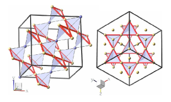
Figure 14: (Color online) Left panel: A-sites of the pyrochlore lattice. Right panel: Kagome lattice formed by layers perpendicular to [111]. From K.A. Ross et al., Physical Review Letters 103, 227202 (2009). http://link.aps.org/abstract/PRL/v103/p227202 Copyright 2009 by the American Physical Society.

The “field cooled” case, $T\to 0$ first, implies for the field directed along [111], $\chi=c=0$ and $M=1/3$, with ${\cal S}=(1/4)k_{\rm B}\ln(4/3)$. The entropy is reduced with respect to the Pauling value, because the ground state degeneracy is partly lifted due to the field directed along [111]. Such a field fixes the direction of the effective spin with the index 0, while three others are free. Such a phase is related to the “Kagome ice” state of the pyrochlore lattice, see Fig. 14. Such a reduction of the entropy due to the external field directed along [111] has been observed [135, 136] in Dy₂Ti₂O₇.

At the critical values of the external magnetic field, directed along [111], the field behavior of the average spin moment shows the jump-like features from the state with the value of the spin moment zero to the value with the average moment 1/3 of the nominal one (1), and then, to the state with the value 1/2 of the nominal (that jump takes place at $g\mu_{\rm B}|\langle J_{z}\rangle|B_{c}=6J$), see Fig. 15.

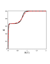
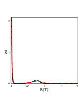
Figure 15: (Color online) The average effective spin moment per rare earth ion $M$ (i.e., it is the magnetization per rare earth ion divided by $g\mu_{\rm B}|\langle J_{z}\rangle|$), right panel, and the magnetic susceptibility $\chi$ (divided by $g\mu_{\rm B}|\langle J_{z}\rangle|/k_{\rm B}$), left panel, as a function of the external field $B$ parallel [111] [for $J=0.8$ K and $T=0.2$ K (solid black curves), and for $T=0.3$ K (dashed red curves) calculated within the Bethe-Peierls approximation for the spin ice model.]

The growing temperature “smears out” those features, slightly shifting the positions of them to higher values of the field. The features near $B=0$ are related to the step-like feature of the magnetic field behavior of the magnetization. It is, in fact, the the manifestation of the transition between the spin ice and Kagome ice phases in the external magnetic field directed along [111]. For other approach to the calculation of magnetization in spin ices in the external [111]-directed magnetic field consult [137].

Figure 16: The average effective spin moment per rare earth ion $M$ as a function of temperature and external magnetic field $B$ directed along [100], calculated for the spin ice model within the Bethe-Peierls approximation. The small features on the surface are artifacts of the numerical computation/drawing.

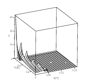
Figure 17: The magnetic susceptibility per rare earth ion $\chi$ (divided by $g^{2}\mu^{2}_{\rm B}|\langle J_{z}\rangle|^{2}/k_{\rm B}$) as a function of temperature and external magnetic field $B$ directed along [100], calculated for the spin ice model within the Bethe-Peierls approximation. The small features on the surface are artifacts of the numerical computation/drawing.

Now let us consider the [100] direction of the applied magnetic field. Here the solution of Eqs. (13) implies the following behavior for the characteristics of the spin-ice system. In the “field-cooled” case the degeneracy is completely lifted and at $T=0$ we should have ${\cal S}=0$. Then the increase of the value of the field results in the “pseudo-transition” [138, 139] from the spin ice state to the “saturated” state. Indeed at $B=B_{K}=\sqrt{(}3)\ln(2)k_{\rm B}T/2g\mu_{\rm B}|\langle J_{z}\rangle|$, a Kasteleyn transition [140, 141], first predicted for the model of dimers on a two-dimensional lattice, takes place from the spin ice phase with the Pauling residual entropy to the “saturated” state with zero entropy and the average effective spin moment a little larger than 1/2 of the nominal value. It happens because one of six spin configurations of “two in - two out” spin ice becomes preferable in such a field, which completely lifts the ground state degeneracy. Notice that this transition is seen in the external magnetic field at the temperature $T=T_{K}=2g\mu_{\rm B}|\langle J_{z}\rangle|B/k_{\rm B}\sqrt{(}3)\ln(2)$: For $T<T_{K}$ the average effective spin moment is about 1/2 of the nominal value, see Fig. 16, and the magnetic susceptibility is zero, see Fig. 17. At $T=T_{k}$ the temperature dependence of the magnetic susceptibility shows a jump-like feature (a cusp in the temperature behavior of the average effective spin moment), and for $T>T_{K}$ both the average moment and the magnetic susceptibility decay with the growth of temperature. The magnetic contribution to the specific heat also manifests features at the Kasteleyn-like transition in its temperature and magnetic field behavior, see Fig. 18. Such a transition has been observed, e.g., [142] in Ho₂Ti₂O₇.

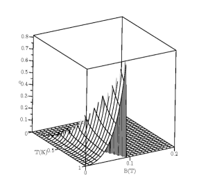
Figure 18: The magnetic contribution to the specific heat per rare earth ion $c$ as a function of temperature and external magnetic field $B$ directed along [100], calculated for the spin ice model within the Bethe-Peierls approximation. The small features on the surface are artifacts of the numerical computation/drawing.

The field along [011] does not affect effective Ising spins 2 and 3, which form $\beta$ chains, and act only on spins, belonging to $\alpha$ chains, see Fig. 10. In the ground state for the “field cooled” case the spin at the position 0 is directed “out”, and the spin at the position 1 is directed “in”, while directions of effective spins from the $\beta$ chain are not fixed. We have at $T=0$ for the “field cooled” case ${\cal S}=c=\chi=0$ and $M=g\mu_{\rm B}|\langle J_{z}\rangle|/\sqrt{6}\approx 0.41g\mu_{\rm B}|\langle J_{z}\rangle|$. The results of calculations of the temperature and magnetic field dependences of the average effective Ising spin and magnetic susceptibility for [011] direction of the field are shown in Figs. 19 and 20. The crossover between the spin ice state and “ordered chain” states has been also observed experimentally [143, 144].

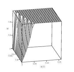
Figure 19: The magnetic moment per rare earth ion $M$ divided by $g^{2}\mu^{2}_{\rm B}|\langle J_{z}\rangle|^{2}/k_{\rm B}$ as a function of temperature and external magnetic field $B$ directed along [011], calculated for the spin ice model within the Bethe-Peierls approximation.

The behavior of thermodynamic characteristics of the spin ice model for other directions of the external field can be calculated in a similar way [134]. It is important to point out that at nonzero values of the field the magnetization of spin ice systems becomes essentially nonzero, which implies the necessity to take into account demagnetization factors of the samples, when comparing theoretical results with the experimentally observed data.

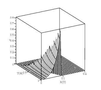
Figure 20: The magnetic susceptibility per rare earth ion $\chi$ (divided by $g^{2}\mu^{2}_{\rm B}|\langle J_{z}\rangle|^{2}/k_{\rm B}$) as a function of temperature and external magnetic field $B$ directed along [011], calculated for the spin ice model within the Bethe-Peierls approximation.

Fig. 21 shows the magnetic field behavior of the magnetization of Dy₂Ti₂O₇ at low temperatures for three different directions of the field. One can see a good agreement of the theory and experimental observations.

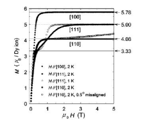
Figure 21: Magnetization of Dy₂Ti₂O₇ as a function of the applied magnetic field applied along [100], [111], and [110] at low temperatures. From H. Fukazawa et al. Physical Review B 65 054410 (2003). http://link.aps.org/abstract/PRB/v65/p054410 Copyright 2003 by the American Physical Society.

Other important experimental results for the magnetic field behavior of Dy₂Ti₂O₇ and Ho₂Ti₂O₇ the reader can find, e.g., in [142, 145, 146, 147, 148, 149, 150, 151, 152, 153, 154, 155, 156, 157, 158, 159].

5.5 Dynamics of spin ices

The dynamical properties of Dy and Ho pyrochlore oxides in the spin ice phase have been intensively studied during the last decade [111, 151, 158, 160, 162, 163, 164, 165, 166, 167, 168, 169, 170, 171, 172].

Figure 22: The temperature dependence of the ac magnetic susceptibility of Dy₂Ti₂O₇. From H. Fukazawa et al., Physical Review B 65, 054410 (2002). http://link.aps.org/abstract/PRB/v65/p054410 Copyright 2002 by the American Physical Society.

Low-temperature (down to 0.06 K) low-frequency (about 10 Hz) measurements of the ac magnetic susceptibility observed that the real part of the dynamical susceptibility becomes lower below about 1 K, while its imaginary part manifests a maximum, see Fig. 22. Below 0.5 K both real and imaginary parts of the dynamical susceptibility have almost zero value, which can be explained by absence of a long-range ordering. Such a behavior is reminiscent of the behavior of the dynamical characteristics of spin glasses [22, 23, 24, 25, 26, 27, 123], for which the difference in the “zero field cooling” and “field cooling” behavior is usual (cf. also the previous section, where we considered static characteristics of spin ices in the external magnetic field). The example of the “zero field cooled” and “field cooled” behavior of the magnetization of Dy₂Ti₂O₇ is shown in Fig. 23. Similar features in the temperature behavior is seen in the real and imaginary part of the dielectric constant, where the external magnetic field strongly affects dynamics [151].

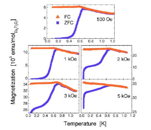
Figure 23: (Color online) The temperature dependence of the magnetization of Dy₂Ti₂O₇ on warming after field cooling (light red curves) and zero field cooling (dark blue curves). From J. Snyder et al., Physical Review B 69, 064414 (2004). http://link.aps.org/abstract/PRB/v69/p064414 Copyright 2004 by the American Physical Society.

The analysis of the temperature behavior of the real and imaginary parts of the dynamical magnetic susceptibility implies the Arrhenius law (while opposite conclusions were also made) [158, 160, 162, 163, 164, 165, 166, 167, 168, 169, 170, 171, 172]. It turns out that the freezing dynamics of spin ice systems differs from the one, associated with spin glasses, where randomness plays, probably, the essential role [22, 23, 24, 25, 26, 27, 123]. For example, the behavior of dynamical characteristics in the external magnetic field for spin ices is very different from the one in spin glasses, where the ordering temperature decreases with the growth of the field value. In Dy₂Ti₂O₇ the temperature of the feature in the dynamical magnetic susceptibility increases with the external field. Also, as expected, the measurements of the dynamical characteristics of spin ices have manifested the anisotropy of properties for the field applied along [111] and [100].

For higher-temperature ($T>4$ K) dynamical characteristics of spin ices also manifest the “freezing” feature about 15 K [158, 160, 162, 163, 164, 165, 166, 167, 168, 169, 170, 171, 172]. The analysis of that behavior implies the presence of the relaxation process with the typical time scales satisfying Arrhenius law $\tau\sim\exp(E_{a}/T)$ with activation energies $E_{a}\sim 200$ K, which agrees with recent muon spin relaxation studies [173, 174], which give the muon relaxation rate of similar form $\propto\exp(-E_{a}/T)$ with $E_{a}\sim 220$ K. It means that such a relaxation involves transitions to the higher-energy single-ion multiplets of rare earth ions. On the other hand, another dynamical processes in spin ices in the temperature range between 5 K and 10 K did not show any significant temperature dependence [173, 174, 175], which has been interpreted as caused by the quantum tunneling effect between up- and down-directed states of effective Ising spins. Notice that $\mu$SR (muon spin relaxation) and ac susceptibility measurements observed relaxation rates different of each other up to three orders of magnitude, perhaps, because of the local character of the $\mu$SR probe. Depolarization of muons is caused mostly by the development on cooling of strong inhomogeneous internal fields (almost static). At very low temperatures, inside the spin ice phase, the residual spin dynamics persists mostly due to the mixture of electron and nuclear energy levels. Spin dynamics in spin ices persists down to lowest temperatures, which fact is observed by several experimental techniques [158, 160, 162, 163, 164, 165, 166, 167, 168, 169, 170, 171, 172, 173, 174, 176]. Magneto-caloric studies of Dy₂Ti₂O₇ revealed extremely slow relaxation [177]. We would like also to mention here the studies of the dynamics of spin ices via the nuclear spin excitation [178], and studies of elastic properties of spin ices [176, 179]. The latter [176] manifested features in the sound characteristics of spin ice systems (sound velocity and attenuation) different for increasing and decreasing external field value, which also implies different relaxation processes in spin ices at low temperatures of order of 0.03 K.

Studies of other representatives of the spin ice family, namely, of stannates, Dy₂Sn₂O₇ and Ho₂Sn₂O₇ were performed in [180, 121, 181, 182].

6 Monopoles as emergent quasiparticles

The interest in spin ices has been considerably grown after the pioneering suggestion that magnetic monopoles can exist as emerging quasiparticles there [183].

In physics, the term “emergence” is used to describe a phenomenon, which can exist at macroscopic scales (in space or time) but not at microscopic scales, despite such a macroscopic system can be considered as a large ensemble of microscopic systems. It is used to distinguish which laws can be applied to macroscopic scales, and which ones only to microscopic scales. Examples of emergent macroscopic characteristics can be a temperature in statistical mechanics, a convection in liquids or gases. Even a mass, space and time in some field theories can be considered as emergent phenomena caused by more fundamental concepts, as strings, branes, or Higgs boson. For the recent example of emergent phenomenon in frustrated magnetic systems, see, e.g., [184].

6.1 Magnetic monopoles

By magnetic monopoles we usually mean a particle that is an isolated magnet with only one magnetic pole. Already in 19th century P. Curie pointed out that magnetic monopoles could exist. However, mainly the problem of magnetic monopoles is associated with P.A.M. Dirac, who has constructed the quantum theory of magnetic monopoles [185]. He has emphasized that quantum mechanics did not preclude the existence of magnetic monopoles, and shown, in particular, that if magnetic monopoles existed, then the electric charge had to be quantized. We know, naturally, that the electric charge is quantized, however this fact, unfortunately, does not prove the existence of magnetic monopoles.

Standard Maxwell’s equations describe magnetism as related to the motion of electric charges (take into account that in quantum mechanics particles can have “intrinsic” magnetic moment related to their spin). The multipole expansion produces first monopole, then dipole, quadrupole, etc. For the electric field the multipole expansion can have the monopole term (charge), while for the magnetic field there is no such a term. That is why, Maxwell’s equations describe electric charges, but not magnetic charges, despite they are symmetric with respect to the interchange of magnetic and electric fields (except of the absence of magnetic charges). On the other hand, we can formally write symmetric Maxwell’s equations, with magnetic monopoles. Two of Maxwell’s equations, Gauss’s law, and Ampère’s law, are not changed (here we use SI units)

$$(\nabla\cdot{\bf E})={\rho_{e}\over\epsilon_{0}}\ ,$$

$$[\nabla\times{\bf B}]=\mu_{0}\epsilon_{0}{\partial{\bf E}\over\partial t}+\mu_{0}{\bf j}_{e}\ ,$$ (16)

where $\rho_{e}$ and ${\bf j}_{e}$ are the electric charge density and electric current density, respectively (notice that the vacuum permittivity is $\epsilon_{0}=c^{-2}\mu_{0}^{-1}=8.85\times 10^{-12}$ F m${-1}$, and ${\bf B}=\mu_{0}{\bf H}$). We can re-write Gauss’s law for magnetism and Faradey’s law of induction in such a way that they become similar to Eqs. (16), namely,

$$(\nabla\cdot{\bf B})=\mu_{0}\rho_{m}\ ,$$

$$-[\nabla\times{\bf E}]={\partial{\bf B}\over\partial t}+\mu_{0}{\bf j}_{m}\ ,$$ (17)

where the magnetic charge density and magnetic current density are introduced. Then the Lorentz force can be presented as

$${\bf F}=q_{e}({\bf E}+[{\bf v}\times{\bf B}])+q_{m}\left({\bf B}-{1\over c^{2}}[{\bf v}\times{\bf E}]\right)\ ,$$ (18)

where $q_{e}$ ($q_{m}$) are the electric (magnetic) charge of a particle, which moves with the velocity ${\bf v}$. For the quantum system, which consists of a single stationary electric charge and a single stationary magnetic charge (monopole), the electromagnetic field, surrounding them, has the momentum density, equal to the Poynting vector ${\bf G}=(1/\mu_{0})[{\bf E}\times{\bf B}]$. It also has the total angular momentum, proportional to $\int d{\bf r}[{\bf r}\times{\bf G}]$, proportional to $q_{e}q_{m}$. The latter is quantized in units of $\hbar$ in quantum mechanics. Then Dirac considered a magnetic charge at the origin, which generates the magnetic field $q_{m}/r^{2}$, directed in the radial direction (analogous to Coulomb’s law). The divergence of ${\bf B}$ is equal to zero almost everywhere, except for the origin at $r=0$. We can locally define the vector potential such that the curl of the vector potential is $[\nabla\times{\bf A}]={\bf B}$. Such vector potential cannot be defined exactly everywhere, because the divergence of the magnetic field is proportional to the Dirac delta function at the origin. Dirac defined one vector potential on the “northern hemisphere” (above the particle), and another one for the “southern hemisphere”. These two vector potentials are matched at the “equator”, and they differ by a gauge transformation. The wave function of an electrically-charged particle that moves around the origin along the “equator” is changed by a phase as in the Aharonov–Bohm-Casher effect. This phase is proportional to the electric charge $q_{e}$ of the moving particle and to the magnetic charge $q_{m}$ of the source. The electric charge returns to the same point after the total trip around the sphere. The phase of its wave function must be unchanged. It implies that the phase added to the wave function must be a multiple of $2\pi$. Hence, Dirac’s quantum theory means quantization of electric and magnetic charges

$$q_{e}q_{m}={2\pi\hbar n\over\mu_{0}}\ ,$$ (19)

where $n$ is an integer. Actually, Dirac’s theory describes an infinitesimal line solenoid as in the Aharonov-Bohm-Casher effect [186, 187], ending at a point. The location of the solenoid is the singular part of the Dirac solution. This line is known now as Dirac’s string. A Dirac string connects monopoles and antimonopoles (magnetic particles with opposite to monopole’s magnetic charge). Dirac strings cannot be seen, because we can put them anywhere. For two coordinate patches, we can made the field in each patch non-singular by sliding the Dirac string to the place, where we cannot observe it. For the recent status of theory and experiment in physics of magnetic monopoles consult [188].

6.2 Magnetic monopoles in spin ices

In condensed matter, and, in particular, in spin ices, we have, of course, $(\nabla\cdot{\bf B})=0$ for the magnetic induction, i.e., no real magnetic monopoles should exist. However, there is no such a restriction on the microscopically determined magnetic field ${\bf H}$. Hence, we can consider quasiparticles, which cannot be constructed as combinations of elementary charges; they can carry fractional charges. Namely such quasiparticles can be monopoles in the terms of ${\bf H}$.

The ground state of the spin ice can be considered as all tetrahedra obeying ice rule (two effective Ising spins are directed “inside” and two directed “outside” of each tetrahedron). Effective spins are constrained to be directed along their local Ising axes ${\bf e}_{n}$, which form the diamond lattice (dual to the original pyrochlore lattice with vertices at the centers of tetrahedra, see Fig. 24) bonds [189]. To remind, the diamond lattice consists of two inter-penetrating FCC sublattices. There is a huge degeneracy of such a state, related to the Pauling entropy. Excitations above such a ground state manifold are defects, which locally violate the ice rule. Using the analogy between the water ice and spin ice [190] we can replace the energy of Ising spins living on pyrochlore lattice sites by the energy of dipoles (dumbbells consisting of equal in value and opposite in sign magnetic charges) that live at the ends of diamond bonds. Let us denote $a_{d}\equiv\sqrt{3/2}a$, which is the diamond lattice constant.

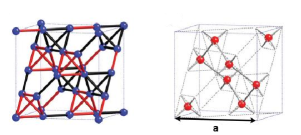
Figure 24: (Color online) Right panel: Original pyrochlore lattice [A-sublattice in light (red); B-sublattice in dark (black)]. Left panel: Dual diamond lattice with bonds defining “easy axes” for total moments of rare earth ions in spin ices. From O. Benton, O. Sikora, and N. Shannon, Physical Review B 86, 075154 (2012). http://link.aps.org/abstract/PRB/v86/p075154 Copyright 2012 by the American Physical Society.

Let us describe how magnetic monopoles can exist in dipolar spin ices following [183]. Consider the Hamiltonian ${\cal H}_{ex}+{\cal H}_{d}$, see Eqs. (4) and (7). A dipole can be thought as a pair of equal and opposite charges $\pm q$ separated by the distance ${\tilde{a}}$, $\mu=q{\tilde{a}}$. Let us choose ${\tilde{a}}=a_{d}$, then magnetic charges are $q=\mu/a_{d}$, where $\mu=g\mu_{\rm B}|\langle J_{z}\rangle|$. The limit ${\tilde{a}}\to 0$ reproduces exactly the Hamiltonian (7). The magnetic Coulomb interaction energy between charges situated at different sites of the diamond lattice is given by

$$v(r_{ij})={\mu_{0}\over 4\pi}{q_{i}q_{j}\over r_{ij}}\ ,$$ (20)

where $r_{ij}$ is the distance between charges, and we can write such an energy for two charges situated at the same site as

$$v(0)=v_{0}q_{i}q_{j}\ ,$$ (21)

where we tune the value of $v_{0}$ to match the interaction energy between two neighboring effective Ising spins on the pyrochlore lattice, $J_{eff}=\pm(J+5D)/3$ (the latter can be obviously obtained when considering one primitive cell). For two neighboring effective spins directed inside the tetrahedron, we get

$$J_{eff}=v(0)-2v(r_{12})-2v(r_{23})+v(r_{13})$$ (22)

where 1, 2, and 3 define the positions of spins (we have $r_{12}=r_{23}=a_{d}$ and $r_{13}=2a$), while for two spins, one of which is directed “in” and the other one “out” we obtain

$$-J_{eff}=-v(0)+2v(r_{12})+2v(r_{23})-v(r_{13})\ .$$ (23)

From these equations we obtain

$$v(0)=J_{eff}+2v(r_{12})-v(r_{13})\ ,$$ (24)

which yields (using the values for charges $|q_{i,j}|=\mu/a_{d}$)

$$v_{0}=\left({a_{d}\over\mu}\right)^{2}\left({J\over 3}+{4D\over 3}\left[1+\sqrt{{2\over 3}}\right]\right)\ .$$ (25)

Then we can introduce the total magnetic charge on each site $n$ of the diamond lattice $Q_{n}=q_{i1}+q_{i2}+q_{i3}+q_{i4}$ for four charges with the coordinates $r_{i,1,2,3,4}=r_{n}$. Then for the Coulomb energy of magnetic charges we can write for $n\neq m$

$$V(r_{nm})={\mu_{0}\over 4\pi}{Q_{n}Q_{m}\over r_{nm}}\ ,$$ (26)

and for $n=m$ we get $V(r_{nn})=v_{0}Q_{n}^{2}/2$, which agrees with the above values for $v(r)$ up to overall constant term $N(\mu/a_{d})^{2}$, where $N$ is the number of dipoles. The energy $v_{0}/2$ is necessary to reproduce correctly the net nearest neighbor interaction. We emphasize that this energy is equivalent to the energy of magnetic dipole-dipole interaction between effective Ising spins, ${\cal H}_{d}$.

Let us first consider the ground state of the dipolar spin ice using the language of such magnetic charges. The total energy has its minimum if each diamond lattice site is neutral, which corresponds to the orientation of dipoles such that $Q_{n}=0$ for each site of the diamond lattice. It is nothing else than the realization of the ice (tetrahedron) rule. Naturally, such a state is degenerate, which yields the Pauling remnant entropy. Then, let us turn to excited states [189]. Naively the most elementary excitation corresponds to the reversing of a single dipole, which generates a local net dipole moment $2\mu$. However, such a simple picture is misleading. The reversed dipole is related to two adjacent sites with the net magnetic charge

$$Q_{n}=\pm{2\mu\over a_{d}}\ ,$$ (27)

which is the nearest neighbor monopole-antimonopole pair. It is easy to see that monopoles can be separated from antimonopoles without violation of the ice rule by reversing a chain of adjacent dipoles, or changing the direction of effective Ising spins on the original pyrochlore lattice [189], see Fig. 25.

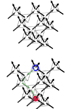
Figure 25: (Color online) Upper panel: Spin ice, which satisfies the spin ice (tetrahedron) rule. Lower Panel: Monopole (blue circle)- antimonopole (red circle) pair. Light (green) arrows show possible Dirac’s string. From Y. Wan and O. Tchernyshyov, Physical Review Letters 108, 247210 (2012). http://link.aps.org/abstract/PRL/v108/p247210 Copyright 2009 by the American Physical Society.

A pair of monopoles separated by the distance $r$ experience a Coulomb magnetic coupling $-\mu_{0}q_{m}^{2}/4\pi r$. It takes only a finite energy to separate monopoles to infinity, which means that monopoles are deconfined. Hence, magnetic monopoles are are true elementary excitations of the spin ice. They are emergent quasiparticles, because of the fractionalization of their charge, see above. The fact that a string of dipoles realizes a monopole-antimonopole pair at its ends is know from the classical electrodynamics [191]. However, it is important that the energy cost of creating such a string of dipoles remains bounded with the growth of its length (the relevant string tension vanishes) to obtain deconfined monopoles. Of course, such a condition cannot be realized in a vacuum, where by growing the length of the string of dipoles we need the energy for creation of additional dipoles. The ice rule can be considered as the requirement that two dipole strings enter and exit each site of the diamond lattice. No domain walls are created along the string in the dipolar spin ice (unlike, e.g, an ordered ferromagnet), which results in the deconfinement of monopoles there.

According to the Dirac quantization condition, the charge of real magnetic monopoles has to be quantized, which is in the close relation to the condition that Dirac’s string is unobservable. On the other hand, the net of (dipole) strings in the dipolar spin ice, which are energetically unimportant, makes dipole strings in such spin ices observable, and the magnetic charge there is not quantized. We can define a density of “smeared” magnetic charges in the dipolar spin ice as

$$\rho_{m}({\bf r})=\int d^{3}{\bf r}^{\prime}(\nabla\cdot{\bf H})e^{-|{\bf r}-{\bf r}^{\prime}|^{2}/\xi^{2}}\ ,$$ (28)

where the monopole at the origin ${\bf r}=0$ separated by $L\gg\xi\gg a$ from other monopoles yields $\rho_{m}(0)=\pm q_{m}$. For the magnetic induction ${\bf B}$, the compensating flux moves along “non-quantized Dirac’s string” of flipped dipoles, created together with each monopoles.

6.3 Properties of magnetic monopoles in spin ices

The external magnetic field applied along [111] acts as a staggered chemical potential for monopoles [183]. We can approximate the low-energy physics of dipolar spin ices as the one of the gas of magnetic monopoles and antimonopoles on the diamond lattice. Hence, one can use the results for such a gas with Coulomb coupling [192]. By changing the value of the chemical potential in that case one can see the temperature crossover between high- and low-density phases at high temperatures, while at low temperatures there must be the first order phase transition between those phases. The line of that phase transition terminates in a critical point in the phase diagram. Notice that for nearest-neighbor spin ice such a liquid-gas transition cannot exist [193], there defects interact only entropically. The low-density phase of the gas of monopoles is related to the Kagome phase in [111] magnetic field, while the high-density phase corresponds to the ordered state with the maximal magnetization along the field direction. Notice that monopoles, which appear in the anomalous Hall effect [194], are not excitations, and involve a real physical magnetic field.

Let us now calculate the equilibrium concentration of monopoles [189]. Each vertex in the diamond lattice at low energies can be in one of 14 states: six monopole-free states (satisfying the ice rule), four states with a monopole, and four states with an antimonopole (three effective Ising spins directed “in” and one “out”, and vice versa). Two states with all effective spins directed “inside” or “outside” the tetrahedron can be ignored in the low energy theory. If $N_{t}$ is the number of tetrahedra, and the number of vertices for each of such states is $N_{i}$ ($i=1,\dots,14$), then the total number of configurations is $N_{t}\!/\prod_{i}N_{i}$ The configurations with parallel and antiparallel effective spins at the midpoints of nearest neighbor bonds (in other words, with correlated and anti-correlated vertices) must not be counted. If the probability of a correlated state is 1/2 then the number of correlated states is $w_{\pm}=(1/2)^{2N_{t}}N_{t}\!/\prod_{i}N_{i}$. If monopoles and antimonopoles are created in pairs, and all states with monopoles and antimonopoles are equivalent $N_{1}=\dots=N_{6}$, $N_{7}=\dots=N_{14}$, the entropy per rare earth ion is $-k_{\rm B}(2x\ln(x)+(1-2x)\ln[2(1-2x)/3])$ where $x=N_{\pm}/N_{t}$ is the concentration of monopoles (antimonopoles) per vertex. The free energy per vertex is then ($\varepsilon_{\pm}$ are the energies of the monopole/antimonopole configurations)

$$f=\varepsilon_{\pm}x+k_{\rm B}T\biggl{[}2x\ln(x)$$

$$+(1-2x)\ln\left({2(1-2x)\over 3}\right)\biggr{]}\ ,$$ (29)

which implies the equilibrium concentration of monopoles being

$$x_{\pm}={2\exp(-\varepsilon_{\pm}/2k_{\rm B}T)\over 3+4\exp(-\varepsilon_{\pm}/2k_{\rm B}T)}\ .$$ (30)

At low temperatures, which is relevant for the experimental situation in spin ice materials, we have $x_{\pm}\approx(2/3)\exp(-\varepsilon_{\pm}/2k_{\rm B}T)$. On the other hand, at high enough temperatures we get, obviously, $x_{\pm}=2/7$.

The monopole picture of spin ices is different from the conventional one in the theory of quasiparticles, because the ground state, as well as excited states for monopoles are highly degenerate. However, for many purposes the information about local configurations is redundant.

Using the analogy between the system of monopoles in the spin ice and water ice it is possible to write the ‘continuity’ equation for the magnetization ${\bf M}$

$${\partial{\bf M}\over\partial t}={Q\over V}(N_{+}{\bf v}_{+}-N_{-}{\bf v}_{-})\ ,$$ (31)

where $Q\equiv Q_{n}$ is the monopole magnetic charge, $V$ is the macroscopically small volume around the point ${\bf r}$, and ${\bf v}_{\pm}$ are the velocities of the monopole and antimonopole. Notice that ${\bf j}_{\pm}={\bf v}_{\pm}N_{\pm}/V$ are densities of currents for monopoles (antimonopoles). The rate of the entropy production due to monopoles (antimonopoles) can be written as

$$T{\partial{\cal S}\over\partial t}=\sum_{\pm}\biggl{[}\pm{\bf j}_{\pm}\biggl{(}Q{\bf H}-{8ak_{\rm B}T{\bf M}\over\sqrt{3}Q}\biggr{)}\biggr{]}\ .$$ (32)

On the other hand, it is equal to $\sum_{\pm}{\bf j}_{\pm}{\bf f}_{\pm}$, where ${\bf f}_{\pm}$ are generalized driving forces. It follows that ${\bf f}_{\pm}=\pm(Q{\bf H}\mp 8ak_{\rm B}T{\bf M}/\sqrt{3}Q)$. The second term describes possible magnetic ordering: When effective spin are partly ordered there exists a nonzero monopole current even without the external field. Then the monopole (antimonopole) currents can be written as

$${\bf j}_{\pm}=\pm u_{\pm}x_{\pm}N_{t}\left(Q{\bf H}-{8ak_{\rm B}T{\bf M}\over\sqrt{3}Q}\right)\ ,$$ (33)

where $u_{\pm}$ are the monopole/antimonopole mobilities, so that $\kappa_{\pm}=u_{\pm}x_{\pm}Q$ are the monopole/antimonopole conductivities. Then it is easy to obtain, taking into account the ‘continuity equation’, that in the linear regime ${\bf M}_{\omega}=\chi(\omega){\bf H}_{\omega}$ with the longitudinal dynamical magnetic susceptibility

$$\chi(\omega)={(\sqrt{3}Q^{2}/8ak_{\rm B}T)\over 1-i\omega\tau}\ ,$$ (34)

where $\tau$ is the relaxation time. The static magnetic susceptibility can be then obtained as

$$\chi_{T}={\sqrt{3}g^{2}\mu_{\rm B}^{2}|\langle J_{z}\rangle|^{2}\over a^{3}k_{\rm B}T}\ ,$$ (35)

The absolute value of the static susceptibility is twice the value of the susceptibility of the standard paramagnet $\chi_{C}$ of the same spin density. This expression for the homogeneous susceptibility has been generalized recently for the inhomogeneous case [195], when taking into account the diffusion of monopoles, as

$$\chi({\bf q},\omega)={\chi_{T}\over 1+(a^{2}q^{2}/6gx)-i\omega\tau}\ ,$$ (36)

where ${\bf q}$ is the wave vector, $x=8a^{3}c/3\sqrt{3}$ is the total dimensionless monopole density ($c$ is the total concentration of monopoles) and $g=\chi_{C}/\chi_{T}$ is the ratio of the static susceptibilities for the spin ice and standard paramagnet; it is equal to 1/2 in the above calculations, however, in general, it can vary from 1 at high temperatures to 1/2 at low temperatures. It implies the correlation length $\xi=a/\sqrt{6gx}$.

If we take into account the demagnetization factor ${\cal D}$ via ${\bf H}_{int}={\bf H}_{ext}-{\cal D}{\bf M}$, the effective susceptibility has to be renormalized as $\chi_{r}\equiv{\bf M}/{\bf H}_{ext}=\chi_{T}/({\cal D}\chi_{T}+1)$. Then the “field cooled” magnetization is just ${\bf M}_{fc}=\chi_{r}{\bf H}_{ext}$, however, the “zero field cooled” one is ${\bf M}_{zfc}=\chi_{r}{\bf H}_{ext}[1-\exp(-t/\tau)]$ (valid at small $t\ll\kappa_{\pm}$), where the time-dependent multiplier comes from the integration of the ‘continuity equation’ for magnetization when we take into account relaxation time $\tau$ and demagnetization factor ${\cal D}$. The behavior of the magnetization derived from that theory [195] is reminiscent of the experimentally observed in spin ices data, presented in Fig. 23.

Closely related problem of magnetic relaxation in spin ices as a “monopole electrolyte” has been studied in [196, 197, 198]. Non-Ohmic conductivity, the Wien effect, [199] for a weak “monopole electrolyte” has been studied theoretically and experimentally by the transverse field low-temperature $\mu$SR [200, 201] (notice, though [202]). Other recent theoretical studies of the dynamical characteristics of monopoles include [203, 204, 205, 206, 207, 208, 209].

Some low-temperature properties of spin ices were successfully described by magnetic monopoles, e.g., in neutron scattering [211, 212], in the behavior of magnetic susceptibility [213] (the latter can be well described by the Debye-Hückel theory [214, 215, 216]), see also [158, 217, 218, 219], in NMR (nuclear magnetic resonance) [220], and in the thermal conductivity [221].

7 Other spin ices

So far we discussed properties of the standard spin ices. However, nowadays physicists consider other possibilities for spin ices.

7.1 Quantum spin ice

By the quantum spin ice we usually mean similar rare earth pyrochlore oxides, in which, unlike usual spin ices, the “easy axes” magnetic anisotropy is not so strong comparing to the spin-spin (total moment-total moment) interaction, like the exchange coupling, or the magnetic dipole-dipole interaction. That is why, there exists a possibility of spreading of a local spin flip to other places due to non-Ising components of the particle-particle interaction [222, 223, 224, 225, 226, 227, 228, 229, 230, 231, 232]. In general, such a possibility can yield magnetic ordering, hence, the level of magnetic frustration for quantum spin ices is lower than for usual ones (sometimes called classical). Strong quantum fluctuations essentially affect statics and dynamics of quantum spin ices. Recent studies show that Yb-based titanate, Yb₂Ti₂O₇, can serve as a good example of a quantum spin ice [233, 234, 235, 236, 237, 238, 239, 240, 241, 242, 243, 244, 245]. Crystalline electric field also well separates the low-energy doublet from other multiplets there. However, planar components of $g$-tensor, $g_{\perp}=4.18$ are larger than longitudinal Ising components (along [111]) $g_{\parallel}=1.77$. Notice that in this compound the anisotropy is also present in exchange interactions with the ferromagnetic $\theta_{\rm CW}\approx 0.65\pm 0.15$ K. The system reveals the phase transition at 0.24 K to the low-temperature phase (the value of the critical temperature depends on the applied magnetic field), which nature has not been totally identified yet, see, e.g. Fig. 26.

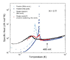
Figure 26: (Color online) The temperature dependence of the specific heat of Yb₂Ti₂O₇ for powder samples (dark and light blue curves) and single crystals (red and black curves). From K.A. Ross et al., Physical Review B 84, 174442 (2011). http://link.aps.org/abstract/PRB/v84/p174442 Copyright 2011 by the American Physical Society.

Most of studies support ferromagnetic ordering in that compound. This phase transition has been recently determined as the Higgs transition from a magnetic Coulomb liquid of monopoles to the ferromagnetic phase, which was viewed as a Higgs phase for magnetic monopoles [246, 247].

7.2 Stuffed spin ice

By stuffed spin ice [84] one means the situation, when magnetic rare-earth ions alter chemically non-magnetic Ti sites, for example Ho³⁺ “stuffs” B-sites like in Ho₂(Ti_2-xHo_x)O_7-δ (where $\delta>0$ implies the balance of oxygen content due to “stuffing”) [248, 249, 250, 251, 252, 253, 254, 255]. Such a procedure, naturally, introduces randomness to the spin ice, and one would expect enhancement of spin glass-like behavior, e.g., the transition to the ordered spin-glass state. The quantum relaxation time is enhanced there, i.e., spin-spin correlations are slower in stuffed spin ices. However, stuffed spin ices do not freeze down to the lowest temperatures, and have basically the same entropy as standard spin ices [248, 249, 250, 251, 252, 253, 254, 255]. On the other hand, stuffed spin ice based on Dy does not manifest residual entropy, i.e., spin fluctuations persist there down to lowest temperatures [219, 256]. Extra spins of Dy-based stuffed spin ice trap magnetic monopoles and obstruct flow of monopoles, introducing residual resistance. For Ho-based stuffed spin ice the ice rules are valid only over a short range. At longer range such a stuffed spin ice exhibits some characteristics of a “cluster glass”, with a tendency to more conventional ferromagnetic correlations.

7.3 Metallic spin ice

We considered above insulating spin ice systems, where the movement of electric charges was absent. Some rare-earth pyrochlore oxides, on the other hand, reveal conducting properties. For example, Pr₂Ti₂O₇ manifests Kondo-like effects (like logarithmic increase of the resistivity and magnetic susceptibility at low temperature) [257, 258, 259]. It is strange, because Pr³⁺ is the Ising ion, and the Ising anisotropy reduces the Kondo screening. Theoretical studies predict that long-range RKKY interaction in metallic pyrochlore oxides should yield magnetic ordering; on the other hand, local spin correlations of the spin ice can produce non-Kondo mechanism of observed features in the temperature dependences [260, 261, 262]. The other metallic spin-liquid system, Pr₂Ir₂O₇ with Ising-like spins along [111] reveals spontaneous Hall effect [258, 263, 264, 265]. There spin-ice correlations in the liquid phase lead to a non-coplanar spin texture forming a uniform but hidden order parameter, the spin chirality.

8 Artificial spin ice

Spin ice is a very interesting system, which, as we have shown above, manifests very rich physics. This is why the study of spin ices has not been limited by natural systems exhibiting spin ice properties. Several years ago the modern lithographic technique was used for the construction of artificial dipolar arrays of single-domain ferromagnetic permalloy Ni_0.81Fe_0.19 islands of a submicron size (with the length of 220 nm, width of 80 nm and thickness of 25 nm) on a Si substrates with a native oxide layer [266]. The moment of each island was about 3$\times 10^{7}\mu_{\rm B}$. Notice that permalloy has effectively zero magnetic anisotropy, so that the anisotropy energy of the island’s magnetic moment itself, which is controlled by it’s shape (of order of 10⁴ K), forced magnetic moments of islands to align along the longer axes, therefore magnetic islands can be considered as effective Ising-like spins. Such arrays of interacting monodomain nanomagnets provide important model systems of statistical mechanics, as they map onto well studied theoretically vertex models, see above. The intrinsic frustration on such a lattice is similar to spin ices. To see how it comes about, we can consider a vortex, where four islands meet. A pair of moments in the vortex can be directed either to maximize or to minimize the magnetic dipole-dipole interaction. It is energetically favorable if the moments of pair of islands are directed in a such a way that one is pointing into the center of the vortex, and the other is directed out of the center of the vortex. On the other hand, the configuration with both moments pointing inside vortex (or outside it) demands additional energy. There are in general 16 configurations of vortices. Six configurations, satisfying the ice rule, with “two-in” and “two out”, like 5 and 6 of Fig. 7 have the lowest energy (the configurations 1, 2, 3 and 4 have higher energies than 5 and 6). On the other hand, the configurations with three moments inside (outside) and four moments inside (outside) the vertex are energetically unfavorable at low temperatures. The energy difference between configurations can be, in principle, regulated by the size of the lattice constant. This approach, in particular, gives the possibility to study the state of the system with local probes, as the magnetic force microscope, to see directly the situation with single constituent magnetic islands, see the example in Fig. 27. Magnetic monodomain permalloy islands that way provide the analogue of effective Ising spins in pyrochlore oxides.

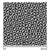
Figure 27: Picture from the magnetic force microscope of the square array of single-domain permalloy magnetic nanoislands. White and black sides of each island show the direction of the magnetic moment of the island. From C. Nisoli et al., Phys. Rev. Lett. 98, 217203 (2007). http://link.aps.org/abstract/PRL/v98/p217203 Copyright 2009 by the American Physical Society.

The construction of artificial frustrated magnet has opened the door to the new approach for the researches with designed artificial systems rather than with natural ones. For example, artificial spin ice systems were proposed to be constructed as arrays of optical traps [267, 268]. A large number of experiments and theories since 2006 have considered artificial spin ice systems, including planes of ferromagnetic islands with square, honeycomb and Kagome lattices [269, 270, 271, 272, 273, 274, 275, 276, 277, 278, 279, 280, 281, 282, 283, 284, 285, 286, 287, 288, 289, 290, 291, 292, 293, 294, 295]. In particular, it has been shown using magneto-optical Kerr effect that disorder in the roughness (in shape) of magnetic islands plays essential role in the collective behavior of artificial spin ices [296, 297]. The interesting study has investigated the behavior of entropy in artificial the spin ice system [298]. The analysis shows that nearest-neighbor correlations drive the longer-range ones there.

As a result of the magnetic frustration, these systems can exhibit magnetic monopole type states, which are an example of an exotic emergent quasiparticle [280, 299, 300, 301, 302, 303, 304, 305, 306, 307, 308, 309, 310, 311]. For example, magnetic monopoles and associated Dirac-like strings have been directly observed in the artificial honeycomb (on Co films of 20 nm thickness) and Kagome spin ice (permalloy films) systems [312, 313, 314] using magnetic force microscopy and X-ray photoemission microscopy. To remind, the Kagome lattice can be realized in pyrochlore spin ices by applying [111] external magnetic field. In particular, for the visualization of magnetic monopoles in permalloy systems the X-ray magnetic circular dichroism was used. Dirac-like strings were observed as a history of propagating monopole-antimonopole pairs. Creation of such pairs as well as their movement has been regulated by the external magnetic field in the reversed (with respect to the magnetic moments of islands) direction. Randomness, as for other artificial spin ices, see above, plays an important role for the physics of monopoles. In contrast to pyrochlore oxides, where magnetic monopoles form a gas and Dirac’s strings are dynamically fluctuating, in an artificial spin ice one deals at large enough values of the external magnetic field with the effective low-temperature case, in which after each field step (change of the magnetization of an island) random variations in the switching field pin monopoles and related Dirac’s strings. Monopoles become trapped. Namely that property permits to image monopole-antimonopole configurations before increasing the value of the field, and to manipulate with such magnetic charges. Dirac’s strings grow in the horizontal or diagonal directions of the two-dimensional lattice as a result of one-dimensional avalanche processes [315].

Artificial spin ices reveal also the anomalous Hall effect [316], which, like in the ferromagnetic SrRuO₃ is believed to be caused by the movement of magnetic monopoles [194].

9 Summary

Studies of magnetic frustrated systems nowadays belong to the one of the most developing branches of the low-temperature condensed matter physics. It is determined by the great variety of new physical concepts, which were applied, and plenty of new physical effects, observed in this field. Spin ices, magnetic monopoles, Higgs effect, anomalous Kondo and Hall physics: All of them have been observed and explained during recent years in frustrated magnets. The studies of magnetic frustrated systems are far from being complete; many new important and interesting effects are waiting for their discoveries. Least but not the last: Frustrated magnets are important not only due to their fundamentally interesting physical properties, but also because of their perspective usefulness as data storages and memories for computers, or as possible realizations of the topological quantum computation.

It is possible that, when reviewing such a swiftly developing field of physics with a great number of important works, and trying to mention all of them, I, perhaps, have not cited some interesting publications. I sincere apologize to those of authors, whose contributions to the field of spin ices and magnetic monopoles there are not mentioned in my article.

I thank R. Moessner for his very helpful comments and suggestions. Support from the Institute for Chemistry of V.N. Karazin Kharkov National University is acknowledged.

Preprinted figures with permission from H. Fukuzawa et al., Physical Review B 65, 054410 (2002); J. Snyder et al., Physical Review B 69, 064414 (2004); J.S. Gardner et al., Physical Review B 70, 180404(R) (2004); X. Ke et al., Physical Review Letters 99, 137203 (2007); C. Nisoli et al., Physical Review Letters 98, 217203 (2007); J.P. Clancy et al., Physical Review B 79, 014408 (2009); K.A. Ross et al., Physical Review Letters 103, 227202 (2009); A. Yaouanc et al., Physical Review B 84, 172408 (2011); K.A. Ross et al., Physical Review B 84, 174442 (2011); Y. Wan and O. Tchernyshyov, Physical Review Letters 108, 247210 (2012); O. Benton, O. Sikora, and N. Shannon, Physical Review B 86, 075154 (2012), Copyrights 2002, 2004, 2007, 2009, 2011, 2012 by the American Physical Society. Readers may view, browse, and/or download material for temporary copying purposes only, provided these uses are for noncommercial personal purposes. Except as provided by law, this material may not be further reproduced, distributed, transmitted, modified, adapted, performed, displayed, published, or sold in whole or part, without prior written permission from the American Physical Society.

References

- [1] See, e.g., D.C. Mattis, The Theory of Magnetism I, Springer, Berlin (1988).
- [2] See, for example, A.A. Zvyagin, Quantum Theory of One-Dimensional Spin Systems, Cambridge Scientific Publishers, Cambridge (2010).
- [3] J.C. Ballhausen, Introduction to Ligand Field Theory, McGraw-Hill, NY (1962).
- [4] J.H. van Vleck, The Theory of Electric and Magnetic Susceptibilities, Oxford University Press, Oxford (1952).
- [5] A. Abragam and B. Bleaney, Electron Paramagnetic Resonance of Transition Ions, Clarendon, Oxford (1969).
- [6] K.W.H. Stevens, Proc. Phys. Soc. A 65, 209 (1952).
- [7] W. Heisenberg, Z. Phys. 49, 619 (1928);
- [8] P.A.M. Dirac, Proc. Roy. Soc. (London) A123, 714 (1929).
- [9] M.A. Ruderman and C. Kittel, Phys. Rev. 96, 99 (1954).
- [10] T. Kasuya, Progr. Theor. Phys. 16, 45 (1956).
- [11] K. Yosida, Phys. Rev. 106, 893 (1957).
- [12] See, e.g., J.S. Smart, Effective Field Theories of Magnetism, W.B. Saunders Company, Phyladelphia, (1966).
- [13] F. Bloch, Z. Phys. 61, 206 (1930).
- [14] T. Holstein and H. Primakoff, Phys. Rev. 58, 1098 (1940).
- [15] L. Néel, Ann. de Phys. 17, 64 (1932);
- [16] L. Nëel, Ann. de Phys. 18, 5 (1932).
- [17] J.H. Conway and N.J.A. Sloane, Sphere Packings, Lattices and Groups, Grundlehren der Mathematischen Wissenschaften 290, Springer-Verlag, Berlin (1999).
- [18] P.W. Anderson, Mater. Sci. Bull. 8, 1008 (1956); Science, 235, 1196 (1987).
- [19] L. Balents, Nature 464, 199 (2010).
- [20] J. Vannimenus and G. Toulouse, J. Phys. C: Solid St. Phys. 10, L537 (1977).
- [21] J. Villain, J. Phys. C: Solid St. Phys. 10, 1717 (1977).
- [22] V. Canella and J.A. Mydosh, Phys. Rev. B 6, 4220 (1972).
- [23] S.F. Edwards and P.W. Anderson, J. Phys. F: Met. Phys. 5, 965 (1975).
- [24] D. Sherington and S. Kirkpatrick, Phys. Rev. Lett. 35, 1792 (1975).
- [25] M. Mezard, G. Parisi, and M.A. Virasoro, Spin glass theory and beyond, World Scientific, Singapore (1987).
- [26] K.H. Fischer and J.A. Hertz, Spin Glasses, Cambridge University Press, Cambridge (1991).
- [27] J.A. Mydosh, Spin Glasses, Taylor & Frensis, NY (1995).
- [28] R.M.F. Houtappel, Physica 16, 425 (1950).
- [29] G.H. Wannier, Phys. Rev. 79, 357 (1950).
- [30] Y. Yafet and C. Kittel, Phys. Rev. 87, 290 (1952).
- [31] Frustrated Spin Systems, Ed.: H.T. Diep, World Scientific, Singapore (2004).
- [32] Highly Frustrated Magnetism, Eds.: C. Lacroix, P. Mendels, and F. Mila, Springer, Berlin (2010).
- [33] A.P. Ramirez, Annu. Rev. Mater. Sci. 24, 453 (1994).
- [34] A.P. Ramirez, Annu. Rev. Mater. Sci. 24, 453 (1994).
- [35] B.D. Gaulin, Hyperfine Interact. 85, 159 (1994).
- [36] P. Schiffer and A.P. Ramirez, Comments Condens. Matter. Phys. 18, 21 (1996).
- [37] J.E. Greedan, J. Matt. Chem. 11, 37 (2001).
- [38] R. Moessner and A.R. Ramirez, Physics Today 59, 24 (2006).
- [39] C. Castelnovo, R. Moessner, and S.L. Sondhi, Ann. Rev. Condens. Matter Phys. 3, 35 (2012).
- [40] A.J. Leadbetter, R.C. Ward, J.W. Clark, P.A. Tucker, T. Matsuo, and S. Suga, J. Chem. Phys. 82, 424 (1985).
- [41] B. J. Murray and A.K. Bertram, Phys.Chem.Chem.Phys. 8, 186 (2006).
- [42] M.J. Iedema, M.J. Dressler, D.L. Doering, J.B. Rowland, W.P. Hess, A.A. Tsekouras, and J.P. Cowin, J. Phys. Chem. B 102, 9203 (1998).
- [43] T.S. Moore and T.F. Winmill, J.Chem. Soc., Trans. 101, 1635 (1912).
- [44] W.M. Latimer and W.H. Rodebush, J. Am. Chem. Soc. 42, 1419 (1920).
- [45] J.D. Bernal and R.H. Fowler, J. Chem. Phys. 1, 515 (1933).
- [46] W.F. Giaque and M.F. Ashley, Phys. Rev. 43, 81 (1933).
- [47] W.F. Giaque and J.W. Stout, J. Am. Chem Soc. 58, 1144 (1936).
- [48] L. Pauling, J. Am. Chem. Soc. 57, 2680 (1935).
- [49] J.F. Nagle, J. Math. Phys. 7, 1484 (1966).
- [50] F. Rys, Helv. Phys. Acta 36, 537 (1963).
- [51] E.H. Lieb, Phys Rev. 162, 162 (1967).
- [52] E.H. Lieb, Phys. Rev. Lett. 18, 692 (1967).
- [53] E.H. Lieb, Phys. Rev. Lett. 19, 108 (1967).
- [54] B. Sutherland, Phys. Rev. Lett. 19, 103 (1967).
- [55] C.P. Yang, Phys. Rev. Lett. 19, 586 (1967).
- [56] J.F. Nagle, Comm. Math. Phys. 13, 62 (1969).
- [57] R.J. Baxter, Exactly solved models in statistical mechanics, Academic Press, London (1982).
- [58] E.J.W. Verwey, Nature 144, 327 (1939).
- [59] E.J.W. Verwey and P.W. Haaymann, Physica 8, 979 (1941).
- [60] P.W. Anderson, Phys. Rev. 102, 1008 (1956).
- [61] S. Kondo, D.C. Johnston, C.A. Swenson, F. Borsa, A.V. Mahajan, L.L. Miller, T. Gu, A.I. Goldman, M.B. Maple, D.A. Gajewski, E.J. Treemann, N.R. Dilley, R.P. Dickey, J. Merrin, K. Kojima, G.M. Luke,Y,J. Uemura, O. Chmaissem, and J.D. Jorgensen, Phys. Rev. Lett. 78, 3729 (1997).
- [62] S. Kondo, D.C. Johnston, and L.L. Miller, Phys. Rev. B 59, 2609 (1999).
- [63] O. Chmaissem, J.D. Jorgensen, S. Kondo, and D.C. Johnston, Phys. Rev. Lett. 79, 4866 (1997).
- [64] V. Eyert, K.H. Hock, S. Horn, A. Loidl, and P.S. Resiborough, Europhys. Lett 46, 762 (1999).
- [65] A. Krimmel, A. Loidl, M. Klemm, S. Horn, and H. Schrober, Phys. Rev. Lett. 82, 2919 (1999).
- [66] P. Fulde, A.N. Yaresko, A.A. Zvyagin, and Y. Grin, Europhys. Lett. 54, 779 (2001);
- [67] J.D. Lee, Phys. Rev. B 67, 153108 (2003).
- [68] Y. Yamashita and K. Ueda, Phys. Rev. B 67, 195107 (2003);
- [69] Y. Matsushita, H. Ueda, Y. Ueda, Nature Materials 4, 845 (2005).
- [70] Y. Shimizu, H. Takeda, M. Tanaka, M. Itoh, S. Niitaka, and H. Takagi, Nature Communications 3, 981 (2012).
- [71] T. Yamada, K. Suzuki, and S. Chikazumi, Appl. Phys. Lett. 13, 172 (1968).
- [72] E.J. Samuelsen, E.J. Bleeker, L. Dobrzynski and T. Riste, J. Appl. Phys. 39, 1114 (1968).
- [73] K. Chiba, K. Suzuki, and S. Chikazumi, J. Phys. Soc. Jpn. Lett. 39, 839 (1975).
- [74] Y. Miyamoto and M. Shindo, J. Phys. Soc. Jpn. 62, 1423 (1993).
- [75] J.P. Wright, J.P. Attfield, and P.G. Radaelli, Phys. Rev. Lett. 87, 266401 (2001).
- [76] P. Fulde, J. Phys.: Condens. Matt. 16, S591 (2003).
- [77] C. Lacroix, Physica B 404, 3038 (2009).
- [78] S.H. Lee, H. Takagi, D. Louca, M. Matsuda, S. Ji, H. Ueda, Y. Ueda, T. Katsufuji, J.H. Chung, S. Park, S.W. Cheong, and C. Broholm, J. Phys. Soc. Jpn. 79, 011004 (2010).
- [79] H. Takagi and S. Niitaka, Highly Frustrated Magnetism in Spinels, In: Introduction to frustrated magnetism: Materials, experiments, theory, Eds. C. Lacroix, P. Mendels, F. Mila, Springer Series in Solid-State Sciences, 164, 155 (2011).
- [80] J. Villain, Z. Phys. B 33, 31 (1979).
- [81] M.A. Subramanian, G. Aravamudan and G.V. Subba Rao, Progr. Sol. State Chem. 15, 55 (1983).
- [82] J.E. Greedan in: Magnetic Properties of Nonmetallic Compounds Based on Transition Elements, Ed. H.P.J. Wijn, Ladolt-Börnstein, New Series, 27, 100 Springer Verlag, Berlin (1992).
- [83] J.E. Greedan, J. Alloys Compd. 408-412 444 (2006).
- [84] J.S. Gardner, M.J.P. Gingras, and J.E. Greedan, Rev. Mod. Phys. 82, 53 (2010).
- [85] M.J.P. Gingras, Spin Ice, in Highly Frustrated Magnetism, Eds.: C. Lacroix, P. Mendels, and F. Mila, Springer, Berlin (2010).
- [86] S. Rosenkranz, A.P. Ramires, A. Hayashi, R.J. Cava, R. Siddharthan, and B.S. Shastry, J. Appl. Phys. 87, 5914 (2000).
- [87] M.J.P. Gingras, B.C. den Hertog, M. Faucher, J.S. Gardner, S.R. Dunsiger, L.J. Chang, B.D. Gaulin, N.P. Raju, and J.E. Greedan, Phys. Rev. B 62, 6496 (2000).
- [88] Y.M. Yana and D. Ghosh, Phys. Rev. B 61, 9657 (2000).
- [89] Y.M. Jana, A. Sengupta, and D. Ghosh, J. Magn. Magn. Mater. 248, 7 (2002).
- [90] I. Mirebeau, P. Bonville, and M. Hennion, Phys. Rev. B 76, 184436 (2007).
- [91] M.T. Hutchings, Solid State Phys. 16, 227 (1964).
- [92] I.D. Ryabov, J. Magn. Reson. 140, 141 (1999).
- [93] C. Rudowicz and C.Y. Chung, J. Phys.: Condens. Matter 16, 5825 (2004).
- [94] S.H. Curnoe, Phys. Rev. B 78, 094418 (2008).
- [95] P.A. McClarty, S.H. Curnoe, and M.J.P.Gingras, J.Phys.: Conf. Ser. 145, 012032 (2009).
- [96] B.C. den Hertog and M.J.P. Gingras, Phys. Rev. Lett. 84, 3430 (2000).
- [97] T. Yavorskii, T. Fennell, M.P.J. Gingras, and S.T. Bramwell, Phys. Rev. Lett. 101, 037204 (2008).
- [98] R. Moessner, Phys. Rev. B 57, R5587 (1998).
- [99] R. Moessner and J.T. Chalker, Phys. Rev. B 58, 12049 (1998).
- [100] R. Siddharthan, B.S. Shastry, and A.P. Ramirez, Phys. Rev. B 63, 184412 (2001).
- [101] S.T. Bramwell, M.J. Harris, B.C. den Hertog, M.J.P. Gingras, J.S. Gardner, D.F. McMorrow, A.R. Wildes, A.L. Cornelius, J.D.M. Champion, R.G. Melko, and T. Fennell, Phys. Rev. Lett. 87, 047205 (2001).
- [102] R. Siddharthan, B.S. Shastry, A.P. Ramirez, A. Hayashi, R.J. Cava, and S. Rosenkranz, Phys. Rev. Lett. 83, 1854 (1999).
- [103] C. Kittel, Introduction to Solid State Physics, Willey, NY (2005).
- [104] R.G. Melko and M.J.P. Gingras, J. Phys.: Condens. Matter 16, R1277 (2004);
- [105] G.T. Barkema, and M.E.J. Newman, Phys. Rev. E 57, 1155 (1998).
- [106] R.G. Melko, B.C. den Hertog, and M.J.P. Gingras, Phys. Rev. Lett. 87, 067203 (2001).
- [107] J.P.C. Ruff, R.G. Melko, and M.G.P. Gingras, Phys. Rev. Lett. 95, 097202 (2005).
- [108] J.N. Reimers, A.J. Berlinsky, and A.C. Shi, Phys. Rev. B 43, 865 (1991).
- [109] M.J.P. Gingras and B.C. den Hertog, Can.J. Phys. 79, 1339 (2001).
- [110] S.V. Isakov, R. Moessner, and S.L. Sondhi, Phys. Rev. Lett. 95, 217201 (2005).
- [111] H. Fukazawa, R.G. Melko, R. Higashinaka, Y. Maeno, and M.J.P. Gingras, Phys. Rev. B 65, 054410 (2002).
- [112] S.V. Isakov, K. Gregor, R. Moessner, and S.L. Sondhi, Phys. Rev. Lett. 93, 167204 (2004).
- [113] C.L. Henley, Phys. Rev. B 71, 014424 (2005).
- [114] V. Khemani, R. Moessner, S.A. Parameswaran, and S.L. Sondhi, Phys. Rev. B 86, 054411 (2012).
- [115] T. Fennell, P.P. Deen, A.R. Wildes, K. Schmalzl, D. Prabhakaran, A.T. Boothroyd, R.J. Aldus, D.F. McMorrow, and S.T. Bramwell, Science 326, 415 (2009).
- [116] M.J. Harris, S.T. Bramwell, D.F. McMorrow, T. Zeiske, and K.W. Godfrey, Phys. Rev. Lett. 79, 2554 (1997).
- [117] M.J. Harris, S.T. Bramwell, T. Zeiske, D.F. McMorrow, and P.J.C. King, J. Magn. Magn. Mater. 177, 757 (1998).
- [118] S.T. Bramwell and M.J.P. Gingras, Science 294, 1495 (2001).
- [119] A.P. Ramirez, A. Hayashi, R.J. Cava, R. Siddharthan, and B.S. Shastry, Nature 399, 333 (1999).
- [120] M. Kanada, Y. Yasui, Y. Kondo, S. Iikubo, M. Ito, H. Harashina, M. Sato, H. Okumura, K. Kakurai, and H. Kadowaki, J. Phys. Soc. Jpn. 71, 313 (2002).
- [121] H. Kadowaki, Y. Ishii, K. Matsuhira, and Y. Hinatsu, Phys. Rev. B 65, 144421 (2002).
- [122] T. Fennell, O.A. Petrenko, B. Fak, J.S. Gardner, S.T. Bramwell, and B. Ouladdiaf, Phys. Rev. B 72, 224411 (2005).
- [123] K. Binder and A.P. Young, Rev. Mod. Phys. 58, 801 (1986).
- [124] S.T. Bramwell and M.J. Harris, J. Phys.: Condens. Matter 10, L215 (1998).
- [125] R. Higashinaka, H. Fukuzawa, D. Yanagishima, and Y. Maeno, J. Phys. Chem Solids 63, 1043 (2002).
- [126] Z. Hiroi, K. Matsuhira, S. Takagi, T. Tayama, and T. Sakakibara, J. Phys. Soc. Jpn. 72, 411 (2003).
- [127] X. Ke, R.S. Freitas, B.G. Ueland, G.C. Lau, M.L. Dahlberg, R.J. Cava, R. Moessner, and P. Schiffer, Phys. Rev. Lett. 99, 137203 (2007).
- [128] A.L. Cornelius and J.S. Gardner, Phys. Rev. B 64, 060406 (2001).
- [129] X. Ke, B.G. Ueland, D.V. West, M.L. Dahlberg, R.J. Cava, and P. Schiffer, Phys. Rev. B 76, 214413 (2007).
- [130] K. Matsuhira, Y. Hinatsu, K. Tenya, and T. Sakakibara, J. Phys.: Condens. Matter 12, L649 (2000).
- [131] K. Matsuhira, C. Sekine, C. Paulsen, and Y. Hinatsu, J. Magn. Magn. Mater. 272-276, E981 (2004).
- [132] H.W.J. Blöte, R.F. Wielinga, and W.J. Huiskamp, Physica 43, 549 (1969).
- [133] D.J. Flood, J. Appl. Phys. 45, 4041 (1974).
- [134] P.N. Timonin, J. Exp. Theor. Phys. 113, 251 (2011).
- [135] Z. Hiroi, K. Matsuhira, S. Takagi, T. Tayama, and T. Sakakibara, J. Phys. Soc. Jpn. 72, 411 (2003).
- [136] R. Higashinaka, H. Fukazawa, and Y. Maeno, Phys. Rev. B 68, 014415 (2003).
- [137] S.V. Isakov, K.S. Raman, R. Moessner, and S.L. Sondhi, Phys. Rev. B 70, 104418 (2004).
- [138] R. Moessner and S.L. Sondhi, Phys. Rev. Lett. 68, 064411 (2003).
- [139] L. Jaubert, J.T. Chalker, P.C.W. Holdsworth, and R. Moessner, Phys. Rev. Lett. 100, 067207 (2008).
- [140] P.W. Kasteleyn, Physica 27, 1209 (1961).
- [141] P.W. Kasteleyn, J. Math. Phys. 4, 287 (1963).
- [142] T. Fenell, S.T. Bramwell, D.F. McMorrow, P. Manuel, and A.R. Wildes, Nature Physics 3, 566 (2007).
- [143] Z. Hiroi, K. Matsuhira, and M. Ogata, J.Phys. Soc. Jpn. 72, 3045 (2003).
- [144] S. Yoshida, K. Nemoto, and K. Wada, J. Phys. Soc. Jpn. 73, 1619 (2004).
- [145] K. Matsuhira, Z. Hiroi, T. Tayama, S. Takagi, and S. Sakakibara, J. Phys.: Condens. Matter 14, L559 (2002).
- [146] O.A. Petrenko, M.R. Lees, and G. Balakrishnan, Phys. Rev. B 68, 012406 (2003).
- [147] T. Sakakibara, T. Tayama, Z. Hiroi, K. Matsuhira, and S. Takagi, Phys. Rev. Lett. 90, 207205 (2003).
- [148] R. Higashinaka, H. Fukazawa, and Y. Maeno, Physica B 329-333, 1040 (2003).
- [149] H. Aoki, T. Sakakibara, K. Matsuhira, and Z. Hiroi, J. Phys. Soc. Jpn. 73, 2851 (2004).
- [150] R. Higashinaka, H. Fukazawa, K. Deguchi, and Y. Maeno, J.Phys. Soc. Jpn. 73, 2845 (2004).
- [151] M. Saito, R. Higashinaka, and Y. Maeno, Phys. Rev. B 72, 144422 (2005).
- [152] R. Higashinaka and Y. Maeno, Phys. Rev. Lett. 95, 237208 (2005).
- [153] Y. Tabata, H. Kadowaki, K. Matsuhira, Z. Hiroi, N. Aso, E. Ressouche, and B. Fak, Phys. Rev. Lett. 97, 257205 (2006).
- [154] J.P. Clancy, J.P.C. Ruff, S.R. Dunsiger, Z. Zhao, H.A. Dabkowska, J.S. Gardner, Y. Qui, J.R.D. Copley, T. Jenkins, and B.D. Gaulin, Phys. Rev. B 79, 014408 (2009).
- [155] B.Z. Malkin, T.T.A. Lummen, P.H.M. van Loosdrecht, G. Dhalenne, and A.R. Zakirov, J. Phys.: Condens. Matter 22, 276003 (2010).
- [156] O.A. Petrenko, M.R. Lees, and G. Balakrishnan, J. Phys.: Condens. Matter 23, 164218 (2011).
- [157] C. Krey, S. Legl, S.R. Dunsiger, M. Meven, J.S. Gardner, J.M. Roper, and C. Pfleiderer, Phys. Rev. Lett. 108, 257204 (2012).
- [158] M.J. Matthews, C. Castelnovo, R. Moessner, S.A. Grigera, D. Prabhakaran, and P. Schiffer, Phys. Rev. B 86, 214419 (2012).
- [159] M.J. Harris, S.T. Bramwell, P.C.W. Holdsworth, and J.D. Champion, Phys. Rev. Lett. 81, 4496 (1998).
- [160] H. Fukazawa and Y. Maeno, J. Phys. Soc. Jpn. 71, 2578 (2002).
- [161] K. Matsuhira, Y. Hinatsu, and T. Sakakibara, J. Phys.: Condens. Matter 13, L737 (2001).
- [162] J. Snyder, J.L. Slusky,R.L. Cava, and P. Schiffer, Nature 413, 48 (2001).
- [163] J. Snyder, B.G. Ueland, J.S. Slusky, H. Karunadasa, R.J. Cava, A. Mizel, and P. Schiffer, Phys. Rev. Lett. 91, 107201 (2003).
- [164] J. Snyder, B.G. Ueland, J.S. Slusky, H. Karunadasa, R.J. Cava, A. Mizel, and P. Schiffer, Phys. Rev. B 69, 064414 (2004).
- [165] J. Snyder, B.G. Ueland, A. Mizel, J.S. Slusky, H. Karunadasa, R.J. Cava, and P. Schiffer, Phys. Rev. B 70, 184431 (2004).
- [166] B.G. Ueland, G.C. Lau, R.J. Cava, J.R. O’Brien, and P. Schiffer, Phys. Rev. Lett. 96, 027216 (2006);
- [167] J.P. Sutter, S. Tsutsui, R. Higashiraka, Y. Maeno, O. Leupold, and A.Q.R. Baron, Phys. Rev. B 75, 140402 (2007).
- [168] K. Kitagawa, R. Higashinaka, K. Ishida, Y. Maeno, and M. Takigawa, Phys. Rev. B 77, 214403 (2008).
- [169] D. Slobinsky, C. Castelnovo, R.A. Borzi, A.S. Gibbs, A.P. Mackenzie, R. Moessner, and S.A. Grigera, Phys. Rev. Lett. 105, 267205 (2010).
- [170] J.A. Quilliam, L.R. Yarashkavitch, H.A. Dabkowska, B.D. Gaulin, and J.B. Kycia, Phys. Rev. B 83, 094424 (2011).
- [171] B. Klemke, M. Meissner, P. Strehlow, K. Kiefer, S.A. Grigera, and D.A. Tennant, J. Low Temp. Phys. 163, 345 (2011).
- [172] C.J. Lin, C.N. Liao, and C.H. Chern, Phys. Rev. B 85, 134434 (2012).
- [173] J. Lago, S.J. Blundell, and C. Baines, J. Phys.: Condens. Matter 19, 326210 (2007).
- [174] P. Quemerais, P. McClarty, and R. Moessnner, Phys. Rev. Lett. 109, 127601 (2012).
- [175] G. Ehlers, A.L. Cornelius, M. Orendac, M. Kajnakova, T. Fennell, S.T. Bramwell, and J.S. Gardner, J. Phys.: Condens. Matter 15, L9 (2003).
- [176] S. Erfanifam, S. Zherlitsyn, J. Wosnitza, R. Moessner, O.A. Petrenko, G. Balakrishnan, and A.A. Zvyagin, Phys. Rev. B 84, 220404(R) (2011).
- [177] M. Orendac, J. Hanko, E. Cizmar, A. Orendacova, M. Shirai, and S.T. Bramwell, Phys. Rev. B 75, 104425 (2007).
- [178] G. Ehlers, E. Mamontov, M. Zamponi, K.C. Kam, and J.S. Gardner, Phys. Rev. Lett. 102, 016405 (2009).
- [179] Y. Nakanishi, T. Kumagai, M. Yoshizawa, K. Matsuhira, S. Takagi, and Z. Hiroi, Phys. Rev. B 83, 184434 (2011).
- [180] T.J. Snee, R.E. Meads, and W.G. Parker, J. Phys. C 10, 1761 (1977); K. Matsuhira, Y. Hinatsu, K. Tenya, H. Amitsuka, and T. Sakakibara, J. Phys. Soc. Jpn. 71, 1576 (2002).
- [181] G. Ehlers, A. Huq, S.O. Diallo, C. Adriano, K.C. Rule, A.L. Cornelius, P. Fouquet, P.G. Pagliuso, and J.S. Gardner, J. Phys.: Condens. Matt. 24, 076005 (2012).
- [182] H.D. Zhou, J.G. Cheng, A.M. Hallas, C.R. Wiebe, G. Li, L. Balicas, J.S. Zhou, J.B. Goodenough, J.S. Gardner, and E.S. Choi, Phys. Rev. Lett. 108, 207206 (2012).
- [183] C. Castelnovo, R. Moessner, and S.L. Sondhi, Nature 451, 42 (2008).
- [184] S.-H. Lee, C. Broholm, W. Ratcliff, G. Gasparovic, Q. Huang, T.H. Kim, and S.-W. Cheong, Nature 418, 856 (2002).
- [185] P.A.M. Dirac, Proc. Roy. Soc. A 133, 60 (1931).
- [186] Y. Aharonov and D. Bohm, Phys. Rev. 115, 485 (1959).
- [187] Y. Aharonov and A. Casher, Phys. Rev. Lett. 53, 319 (1984).
- [188] K.A. Milton, Rep. Prog. Phys. 69, 1637 (2006).
- [189] I.A. Ryzhkin, J. Exp. Theor. Phys. 101, 481 (2005).
- [190] J.F. Nagle, Chem. Phys.43, 317 (1979).
- [191] J.D. Jackson, Classical Electrodynamics, Wiley, NY (1975).
- [192] V. Kobelev, A.B. Kolomeisky and M.E. Fisher, J. Chem. Phys. 116, 7589 (2002).
- [193] O.J. Heilmann and E.H. Lieb, Comm. Math. Phys. 25, 190 (1972).
- [194] Z. Fang, N. Nagaosa, K.S. Takahashi, A. Asamitsu, R. Mathieu, T. Ogasawara, H. Yamada, M. Kawasaki, Y. Tokura, and K. Terakura, Science 302, 92 (2003).
- [195] S.T. Bramwell, Phil. Trans. Roy. Soc. A 370, 5738 (2012).
- [196] R. Moessner and P. Schiffer, Nature Physics 5, 250 (2009).
- [197] L.D.C. Jaubert and P.C.W. Holdsworth, Nature Physics 5, 258 (2009).
- [198] L.D.C. Jaubert and P.C.W. Holdsworth, J. Phys.: Condens. Matter 23, 164222 (2011).
- [199] L. Onsager, J. Chem. Phys. 2, 599 (1934).
- [200] S.T. Bramwell, S.R. Giblin, S. Calder, R. Aldus, D. Prabhakaran, and T. Fennell, Nature 461, 956 (2009).
- [201] S.R. Giblin, S.T. Bramwell, P.C.W. Holdsworth, D. Prabhakaran, and I. Terry, Nature Physics 7, 252 (2011).
- [202] S.R. Dunsiger, A.A. Aczel, C. Arguello, H.A. Dabkowska, A. Dabkowski, M.H. Du, T. Goko, B. Javanparast, T. Lin, F.L. Ning, H.M.L. Noad, D.J. Singh, T.J. Williams, Y. J. Uemura, M.J.P. Gingras, and G.M. Luke, Phys. Rev. Lett. 107, 207207 (2011).
- [203] S.T. Bramwell, J. Phys.: Condens. Matter 23, 112201 (2011).
- [204] A.V. Shtyk and M.V. Feigelman, JETP lett. 92, 799 (2010).
- [205] I.A. Ryzhkin and M.I. Ryzhkin, JETP Lett. 93, 384 (2011).
- [206] I.A. Ryzhkin, A.V. Klyuev, M.I. Ryzhkin, and I.V. Tsybulin, JETP Lett. 95, 302 (2012).
- [207] S.J. Blundell, Phys. Rev. Lett. 108, 147601 (2012).
- [208] A. Takeuchi and G. Tatara, J. Appl. Phys. 111, 07C509 (2012).
- [209] P. Strehlow, S. Neubert, B. Klemke, and M. Meissner, Cont. Mech. Therm. 24, 347 (2012).
- [210] M.J.P. Gingras, Science 326, 375 (2009).
- [211] D.J.T. Morris, D.A. Tennant, S.A. Grigera, B. Klemke, C. Castelnovo, R. Moessner, C. Czternasty, M. Meissner, K.C. Rule, J.-U. Hoffmann, K. Kiefer, S. Gerischer, D. Slobinsky, and R.S. Perry, Science 326 411 (2009).
- [212] T. Fennell, P.P. Deen, A.R. Wildes, K. Schmalzl, D. Parabharkan, A.T. Boothroyd, R.J. Aldus, D.F. McMarrow, and S.T. Bramwell, Science, 326 415 (2009).
- [213] H. Kadowaki, N. Doi, Y. Aoki, Y. Tabata, T.J. Sato, J.W. Lynn, K. Matsuhira, and Z. Hiroi, J. Phys. Soc. Jpn. 78, 103706 (2009).
- [214] C. Castelnovo, R. Moessner, and S.L. Sondhi, Phys. Rev. Lett. 104, 107201 (2010).
- [215] H.D. Zhou, S.T. Bramwell, J.G. Cheng, C.R. Wiebe, G. Li, L. Balicas, J.A. Bloxsom, H.J. Silverstein, J.S. Zhou, J.B. Goodenough, and J.S. Gardner, Nature Commun. 2, 478 (2011).
- [216] C. Castelnovo, R. Moessner, and S.L. Sondhi, Phys. Rev. B 84, 144435 (2011).
- [217] J.A. Quilliam, L.R. Yaraskavitch, H.A. Dabkowska, B.D. Gaulin, and J.B. Kycia, Phys. Rev. B 83, 094424 (2011).
- [218] L.R. Yaraskavitch, H.M. Revell, S. Meng, K.A. Ross, H.M.L. Noad, H.A. Dabkowska, B.D. Gaulin, and J.B. Kycia, Phys. Rev. B 85, 020410(R) (2012).
- [219] H.M. Revell, L.R. Yaraskavitch, J.D. Mason, K.A. Ross, H.M.L. Noad, H.A. Dabkowska, B.D. Gaulin, P. Henelius, and J.B. Kycia, Nature Physics 9, 34 (2013).
- [220] G. Sala, C. Castelnovo, R. Moessner, S.L. Sondhi, K. Kitagawa, M. Takigawa, R. Hagashinaka, and Y. Maeno, Phys. Rev. Lett. 108, 217203 (2012).
- [221] G. Kolland, O. Breunig, M. Valldor, M. Hiertz, J. Frielingsdorf, T. Lorenz, Phys. Rev. B 86, 060402(R) (2012).
- [222] R. Moessner, Can. J. Phys. 79, 1283 (2001).
- [223] A.G. Del Maestro and M.J.P. Gingras, J. Phys.: Condens. Matter 16, 3339 (2004).
- [224] R. Moessner, O. Tchernyshyov, and S.L. Sonhi, J. Stat. Phys. 116, 755 (2004).
- [225] F.J. Burnell, S. Chakravarty, and S.L. Sondhi, Phys. Rev. B 79, 144432 (2009).
- [226] S. Maegawa, A. Oyamada, and S. Sato, J. Phys. Soc. Jpn. 79, 011002 (2010).
- [227] S. Onoda and Y. Tanaka, Phys. Rev. B 83, 094411 (2011).
- [228] K.A. Ross, L. Savary, B.D. Gaulin, and L. Balents, Phys. Rev. X 1, 021002 (2011).
- [229] N. Shannon, O. Sikora, F. Pollmann, K. Penc, and P. Fulde, Phys. Rev. Lett. 108, 067204 (2012).
- [230] Y. Wan and O. Tchernyshyov, Phys. Rev. Lett. 108, 247210 (2012).
- [231] O. Benton, O. Sikora, and N. Shannon, Phys. Rev. B 86, 075154 (2012).
- [232] S. Lee, S. Onoda, and L. Balents, Phys. Rev. B 86, 104412 (2012).
- [233] J.A. Hodges, P. Bonville, A. Forget, M. Rams, K. Krolas, and G. Dhalenne, J. Phys. Condens. Matter 13, 9301 (2001).
- [234] J.A. Hodges, P. Bonville, A. Forget, A. Yaouanc, P. Dalmas de Reotier, G. Andre, M. Rams, K. Krolas, C. Ritter, P.C.M. Gubbens, C.T. Kaiser, P.J.C. King, and C. Baines, Phys. Rev. Lett. 88, 077204 (2002).
- [235] K.A. Ross, J.P.C. Ruff, C.P. Adams, J.S. Gardner, H.A. Dabkowska, Y. Qiu, J.R.D. Copley, and B.D. Gaulin, Phys. Rev. Lett. 103, 227202 (2009).
- [236] Y. Yasui, M. Soda, S. Iikubo, M. Ito, M. Sato, N. Hamaguchi, T. Matsushita, N. Wada, T. Takeuchi, N. Aso, and K. Kakurai, J. Phys. Soc. Jpn. 72, 3014 (2003).
- [237] J.S. Gardner, G. Ehlers, N. Rosov, R.W. Erwin, and C. Petrovic, Phys. Rev. B 70, 180404(R) (2004).
- [238] H.B. Cao, A. Gukasov, I. Mirebeau, and P. Bonville, J. Phys.: Condens. Matter 21, 492202 (2009).
- [239] A. Yaouanc, P. Dalmas de Reotier, C. Marin, and V. Glazkov, Phys. Rev. B 84, 172408 (2011).
- [240] K.A. Ross, L.R. Yaraskavitch, M. Laver, J.S. Gardner, J.A. Quilliam, S. Meng, J.B. Kycia, D.K. Singh, Th. Proffen, H.A. Dabkowska, and B.D. Gaulin, Phys. Rev. B 84, 174442 (2011).
- [241] J.D. Thompson, P.A. McClarty, H.M. Ronnow, L. P. Regnault, A. Sorge, and M.J.P. Gingras, Phys. Rev. Lett. 106, 187202 (2011).
- [242] J.D. Thompson, P.A. McClarty, and M.J.P. Gingras, J. Phys.: Condens. Matter 23, 164219 (2011).
- [243] K.A. Ross, Th. Proffen, H.A. Dabkowska, J.A. Quilliam, L.R. Yaraskavitch, J.B. Kycia, and B.D. Gaulim, Phys. Rev. B 86, 144424 (2012).
- [244] E. Lhotel, C. Paulsen, P.D. de Reotier, A. Yaouanc, C. Marin, and S. Vanishri, Phys. Rev. B 86, 020410(R) (2012).
- [245] R. Applegate, N.R. Hayre, R.R.P. Singh, T. Lin, A.G.R. Day, and M.J.P. Gingras, Phys. Rev. Lett. 109, 097205 (2012).
- [246] S. Powell Phys. Rev. B 84, 094437 (2011).
- [247] L.J. Chang, S. Onoda, Y.X. Su, Y.J. Kao, K.D. Tsuei, Y.K. Yasui, K. Kakurai, and M.R. Lees, Nature Commun. 3, 992 (2012).
- [248] G.C. Lau, R.S. Freitas, B.G. Ueland, B.D. Muegge, E.L. Duncan, P.Schiffer, and R.J. Cava, Nature Physics 2, 249 (2006).
- [249] G.C. Lau, B.D. Muegge, T.M. McQueen, E.L. Duncan, and R.J. Cava, J. Solid State Chem. 179, 3126 (2006).
- [250] G.C. Lau, R.S. Freitas, B.G. Ueland, M.L. Dahlberg, Q. Huang, H.W. Zandbergen, P. Schiffer, and R.J. Cava, Phys. Rev. B 76, 054430 (2007).
- [251] H.D. Zhou, C.R. Wiebe, Y.J. Jo, L. Balicas, Y. Qiu, J.R.D. Copley, G. Ehlers, P. Fouquet, and J.S. Gardner, J. Phys.: Condens. Matt. 10, 342201 (2007).
- [252] G.C. Lau, T.M. McQueen, Q. Huang, H.W. Zandbergen, and R.J. Cava, J. Solid State Chem. 181, 45 (2008).
- [253] G. Ehlers, J.S. Gardner, Y. Qiu, P. Fouquet, C.R. Wiebe, L. Balicas, and H.D. Zhou, Phys. Rev. B 77, 052404 (2008).
- [254] J.S. Gardner, G. Ehlers, P. Fouquet, B. Farago, and J.R. Stewart, J. Phys.: Condens. Matter 23, 164220 (2011).
- [255] R.J. Aldus, T. Fennell, P.P. Deen, E. Ressouche, G.C. Lau, R.J.Cava, and S.T. Bramwell, New J. Phys. 15 013022 (2013).
- [256] B.G. Ueland, G.C. Lau, R.S. Freitas, J. Snyder, M.L. Dahlberg, B.D. Muegge, E.L. Duncan, R.J. Cava, and P. Schiffer, Phys. Rev. B 77, 020405(R) (2008).
- [257] D. Yanagishima, and Y. Maeno, J. Phys. Soc. Jpn. 70, 2880 (2001).
- [258] S. Nakatsuji, Y. Machida, Y. Maeno, T. Tayama, T. Sakakibara, J. van Duijn, L. Balicas, J.N. Millican, R.T. Macaluso, and J.Y. Chan, Phys. Rev. Lett. 96, 087204 (2006).
- [259] Y. Machida, S. Nakatsuji, Y. Maeno, T. Tayama, T. Sakakibara, and S. Onoda, Phys. Rev. Lett. 98, 057203 (2007).
- [260] A. Ikeda and H. Kawamura, J. Phys. Soc. Jpn. 77 073707 (2008).
- [261] M. Udagawa, H. Ishizuka, and Y. Motome, Phys. Rev. Lett. 108, 066406 (2012).
- [262] H. Ishizuka, M. Udagawa, and Y. Motome, J. Phys. Soc. Jpn. 81, 113706 (2012)
- [263] Y. Machida, S. Nakatsuji, H. Tonomura, T. Tayama, T. Sakakibara, J. van Duijn, C. Broholm, and Y. Maeno, J. Phys. Chem. Solids 66, 1435 (2005).
- [264] J.N. Millican, R.T. Macaluso, S. Nakatsuji, Y. Machida, Y. Maeno, and J.Y. Chan, Mater. Res. Bull. 42, 928 (2007).
- [265] Y. Machida, S. Nakatsuji,S. Onda, T. Tayama, and T. Sakakibara, Nature 463, 210 (2010).
- [266] R.F. Wang, C. Nisoli, R.S. Freitas, J. Li. W. McConville, B.J. Cooley, M.S. Lund, N. Samarth, C. Leighton, V.H. Crespi, and P. Schiffer, Nature 439, 303 (2006).
- [267] A. Libal, C. Reichhardt, and C.J.O. Reichhardt, Phys. Rev. Lett. 97, 228302 (2006).
- [268] J. Struck, C. Ölschläger, R. Le Targat, P. Soltan-Panahi, A. Eckardt, M. Lewenstein, P. Windpassinger, and K. Sengstock, Science 333, 996 (2011).
- [269] C. Nisoli, R.F. Wang, J. Li, W.F. McConville, P.E. Lammert, P. Schiffer, and V.H. Crespi, Phys. Rev. Lett. 98, 217203 (2007).
- [270] A. Leon and J. Pozo, J. Magn. Magn. Mater. 320, 210 (2008).
- [271] Y. Qi, T. Brintlinger, and J. Cumings, Phys. Rev. B 77, 094418 (2008).
- [272] E. Mengotti, L.J. Heyderman, A. Fraile Rodriguez, A. Bisig, L. Le Guyader, F. Nolting, and H.B. Braun, Phys. Rev. B 78, 144402 (2008).
- [273] A. Trabesinger, Nature Physics 4, 832 (2008).
- [274] A. Libal, C.J.O. Reichhardt, and C. Reichhardt, Phys. Rev. Lett. 102, 237004 (2009).
- [275] J. Li, X. Ke, S. Zhang, D. Garand, C. Nisoli, P. Lammert, V.H. Crespi, and P. Schiffer, Phys. Rev. B 81, 092406 (2010).
- [276] Z. Budrikis, P. Politi, and R.L. Stamps, Phys. Rev. Lett. 105, 017201 (2010).
- [277] A. Schumann, B. Sothmann, P. Szary, and H. Zabel, Appl. Phys. Lett. 97, 022509 (2010).
- [278] C. Nicoli, J. Li, X.L. Ke, D. Garand, P. Schiffer, and V.H. Crespi, Phys. Rev. Lett. 105, 047205 (2010).
- [279] O. Tchernyshyov, Nature Phys. 6, 323 (2010).
- [280] P. Mellado, O. Petrova, Y.C. Shen, and O. Tchernyshyov, Phys. Rev. Lett. 105, 187206 (2010).
- [281] Y. Li and T.X. Wang, Phys. Lett. A 374, 4475 (2010).
- [282] J. Li, S. Zhang, J. Bartell, C. Nisoli, X. Ke, P.E. Lammetr, V.H. Crespi, and P. Schiffer, Phys. Rev. B 82, 134407 (2010).
- [283] N. Rouemaille, F. Montaigne, B. Canals, A. Duluard, D. Lacour, M. Hehn, R. Belkhou, O. Fruchart, S. el Moussaoui, A. Bendounan, and F. Maccherozzi, Phys. Rev. Lett. 106, 057209 (2011).
- [284] Y. Li, T.X. Wang, H.Y. Liu, X.F. Dai, and G.D. Liu, Phys. Lett. A 375, 1548 (2011).
- [285] S.A. Daunheimer, O. Petrova, O. Tchernyshyov, and J. Cumings, Phys. Rev. Lett. 107, 167201 (2011).
- [286] Z. Budrikis, P. Politi, and R.L. Stamps, Phys. Rev. Lett. 107, 217204 (2011).
- [287] C.J.O. Reichhardt, A. Libal, and C. Reichhardt, New J. Phys. 14, 025006 (2012).
- [288] V. Kapaklis, U.B. Arnalds, A. Harman-Clarke, E.T. Papaioannou, M. Karimipour, P. Korelis, A. Taroni, P.C.W. Holdsworth, S.T. Bramwell, and B. Hjorvarsson, New J. Phys. 14, 035009 (2012).
- [289] A. Scumann, P. Szari, E.Y. Vedmedenko, and H. Zabel, New J. Phys. 14, 035015 (2012);
- [290] K. Budrikis, K.L. Livesey, J.P. Morgan, J. Akerman, A. Stein, S. Langridge, C.H. Marrows, and R.L. Stamps, New J. Phys. 14, 035014 (2012).
- [291] Z. Budrikis, P. Politi, and R.L. Stamps, J. Appl. Phys. 111, 07E109 (2012).
- [292] L.A.S. Mol, A.R. Pereira, and W.A. Moura-Melo, Phys. Rev. B 85, 184410 (2012).
- [293] S. Zhang, J. Li, I. Gilbert, J. Bartell, M.J. Erikson, Y. Pan, P.E. Lammert, C. Nisoli, K.K. Kohli, R. Misra, V.H. Crespi, N. Samarth, C. Leighton, and P. Schiffer, Phys. Rev. Lett. 109, 087201 (2012).
- [294] U.B. Arnalds, A. Farhan, R.V. Chopdekar, V. Kapaklis, A. Balan, E.T. Papaioannou, M. Ahlberg, F. Nolting, L.J. Heyderman, and B. Hjorvarsson, Appl. Phys. Lett. 101, 112404 (2012).
- [295] J.P. Morgan, J. Akerman, A. Stein, C. Phatak, R.M.L. Evans, S. Langridge, and C.H. Marrows, Phys. Rev. B 87, 024405 (2013).
- [296] K.K. Kohli, A.L. Balk, J. li, S. Zhang, I. Gilbert, P.E. Lammert, V.H. Crespi, P. Schiffer, and N. Samarth, Phys. Rev. B 84, 180412(R) (2011).
- [297] Z. Budrkis, J.P. Morgan, J. Akerman, A. Stein, P. Politi, S. Langridge, C.H. Marrows, and R.L. Stamps, Phys. Rev. Lett. 109, 037203 (2012).
- [298] P.E. Lammert, X.L. Ke, J. Li, C. Nisoli, D.M. Garand, V.H. Crespi, and P. Schiffer, Nature Phys. 6, 786 (2010).
- [299] G. Möller and R. Moessner, Phys. Rev. Lett. 96, 237202 (2006).
- [300] L.A. Mol, R.L. Silva, R.C. Silva, A.R. Pereira, W.A. Moura-Melo, and B.V. Costa, J. Appl. Phys. 106, 063913 (2009).
- [301] G. Möller and R. Moessner, Phys. Rev. B 80, 140409(R) (2009).
- [302] G. Rosenberg and M. Franz, Phys. Rev. B 82, 035105 (2010).
- [303] J.P. Morgan, A. Stein, S. Langridge, and C.H. Marrows, Nature Physics 7, 75 (2011).
- [304] S. Ladak, D. Read, T. Tyliszczak, W.R. Branford, and L.F. Cohen, New J. Phys. 13, 023023 (2011).
- [305] C. Phatak, A.K. Petford-Long, O. Heinonen, M. Tanase, and M. De Graef, Phys. Rev. B 83, 174431 (2011).
- [306] S. Ladak, D.E. Read, W.R. Branford, and L.F. Cohen, New J. Phys. 13, 063032 (2011).
- [307] J.P. Morgan, A. Stein, S. Langridge, and C.H. Marrows, New J. Phys. 13, 105002 (2011).
- [308] R.C. Silva, F.S. Nascimento, L.A.S. Mol, W.A. Moura-Melo,and A.R. Pereira, New J. Phys. 14, 015008 (2012); C. Nisoli, New J. Phys. 14, 035017 (2012).
- [309] R.V. Hugli, G, Duff, B. O’Conchuir, E. Mengotti, L.J. Heyderman, A.F. Rodriguez, F. Nolting, and H.B. Braun, J. Appl. Phys. 111, 07E103 (2012).
- [310] S.D. Pollard, V. Volkov, and Y. Zhu, Phys. Rev. B 85, 180402(R) (2012);
- [311] R.C. Silva, R.J.C. Lopes, L.A.S. Mol, W.A. Moura-Melo, G.M. Wysin, and A.R. Pereira, Phys. Rev. B 87, 014414 (2013).
- [312] S. Ladak, D.E. Reaf, G.K. Perkins, L.F. Cohen, and W.R. Branford, Nature Phys. 6, 359 (2010).
- [313] E. Mengotti,L.J. Heyderman, A.F. Rodriguez, F. Nolting, R.V. Hugli, and H.B. Braun, Nature Physics 7, 68 (2011).
- [314] J. Cumings, Nature Physics 7, 7 (2011).
- [315] J.P. Setha, K.A. Dahmen and C.R. Myers, Nature 410, 242 (2001).
- [316] W.R. Branford, S. Ladak, D.E. Read, K. Zeissler, and L.F. Cohen, Science, 335, 1597 (2012).