Integrable two layer point vortex motion on the half plane

Abstract.

In this paper we derive the equations of motion for two-layer point vortex motion on the upper half plane. We study the invariants using symmetry, including the Hamiltonian and show that the two vortex problem is integrable. We characterize all two vortex motions for the cases where the vortex strengths are both equal, $\Gamma_{1}=\Gamma_{2}=1$ and when they are opposite $\Gamma_{1}=-\Gamma_{2}=1$. We also prove that there are no equilibria for the two vortex problem when $\Gamma_{1}=-\Gamma_{2}=1$. We show that there is only one relative equilibrium configuration when $\Gamma_{1}=\Gamma_{2}=1$ and the vortices are in different layers. We also make observations concerning the finite-time collapse of two vortices in the half plane. We then compare the regimes of motion for both cases (motion on the half plane) with the case of the two-layer vortex problem on the entire plane. We also study several classes of streamline topologies for two vortices in different layers. We conclude with a Hamiltonian study of integrable two-layer 3 vortex motion on the half plane by studying integrable symmetrical configurations and provide a rich class of new relative equilibria.

1.
Introduction

There is a vast literature on $N$-body vortex problems, much of which is reference in the book by Newton [14]. The geostrophic vortex models are described in many geophysics texts including [15]. There has been some work done on two-layer point vortex dynamics on the entire plane. These include the works of Young [16], and Hogg and Stommel [5][6] , and which have been primarily numerical investigations. Some experimental work has been done by Griffiths and Hopfinger [3]. More analytic results can be found in the work of Gryanik [4] and Zabusky and McWilliams [12] and Flierl,  Polvani and Zabusky [1].  Integrable two layer point vortex motion in the plane has been extensively studied by Jamaloodeen and Newton [7][9]. More recent studies can also be found in the works of Koshel et al [10][11]. In these are studied the equilibrium solutions, the vortex collapse problem and the transition to chaotic advection through perturbations of known equilibrium solutions. The two layer vortex problem in domains other than the entire plane has not been as extensively studied as the one layer vortex problem on domains with boundaries.  A good exposition of the one layer vortex problem on domains with boundaries can be found in work of Flucher and Gustafsson[2]. The work in this study can be understood as applying the techniques for one layer integrable vortex dynamics on domains with boundaries [2], and the analytic techniques for integrable two layer vortex dynamics in the unbounded plane [7][9][10][11], to integrable two layer vortex dynamics in the upper half plane.

This paper is organized as follows. We begin by deriving the equations of motion, by first obtaining the streamfunctions for an ensemble of point vortices.  We also obtain the invariants through the use of symmetry and establish the integrability of the two vortex problem in the upper half plane. Through analysis of the Hamiltonian energy curves we characterize all 2 point vortex motion in the upper half plane for both cases $\Gamma_{1}=$ $\Gamma_{2}=1$ and $\Gamma_{1}=$ $-\Gamma_{2}=1$ including conclusions about 2 vortex collapse. We then determine all equilibrium solutions for the 2 point vortex motion, again, for both cases. We proceed by comparing the Hamiltonian energy curves for the two layer problem in upper half plane with the one layer problem in the upper half plane. We then present qualitative aspects of streamline topologies for the two layer problem, for both cases $\Gamma_{1}=$ $\Gamma_{2}=1$ and $\Gamma_{1}=$ $-\Gamma_{2}=1$.  We conclude with a study of integrable 3 vortex motion by considering symmetrical initial configurations, and seeking conditions to maintain the symmetry of the initial configuration. By enforcing those conditions, which simplify by symmetry of the configuration, we are able to obtain, numerically, rich classes of relative equilibria in both cases $\Gamma_{1}=$ $\Gamma_{2}=1$ and $\Gamma_{1}=$ $-\Gamma_{2}=1$.

2.
Equations of motion and invariants

We consider first an ensemble of two point vortices in the upper half plane where $\Gamma_{1}$ is in bottom layer and $\Gamma_{2}$ is in top. Denoting the respective stream functions in the corresponding layers by $\psi_{i}$ ($i=1,2$) the expession for determining the streamfunctions corresponding to unit (delta) point vortices $\delta_{i}(\varsigma)$ in each of the two layers are

(1a) $$\Delta\psi_{1}-k^{2}(\psi_{1}-\psi_{2}) =\delta_{1}(\zeta),$$

(1b) $$\Delta\psi_{2}+k^{2}(\psi_{1}-\psi_{2}) =\delta_{2}(\zeta),$$

where the subscripts identify the layer and $1/k$ is the internal radius of deformation.  These equations apply here to the domain $D$, the upper half plane with boundary $y=0$, and boundary conditions $\psi_{i}|_{\partial D}=0$. By introducing the sum and differences $\psi=\psi_{1}+\psi_{2}$ and $\varphi=\psi_{1}-\psi_{2}$ the equations (1) uncouple

(2a) $$\Delta\psi =\delta_{1}+\delta_{2}=\delta(\zeta)$$

(2b) $$\Delta\varphi-k^{2}\varphi =\delta_{1}-\delta_{2}=\delta^{\prime}(\zeta)$$

The fundamental solution of (2a) on the half plane is obtained, through the method of images [13], using the Green’s function,

(3) $$G(z;\zeta)=G(x,y;\xi,\eta)=\ln\left|z-\zeta\right|-\ln\left|z-\overline{\zeta}\right|\text{.}$$

The fundamental solution of (2b) on the half plane is obtained using the Green’s function

(4) $$G(z;\zeta)=G(x,y;\xi,\eta)=K_{0}\left(k\left|z-\zeta\right|\right)-K_{0}\left(k\left|z-\overline{\zeta}\right|\right)$$

with $K_{0}\left(x\right)$ the modified Bessel function using the complex variable notation,

$$z=x+iy\text{ and }\zeta=\xi+i\eta\text{.}$$

In this study we restrict the radius of deformation to be $1$ so that $k=1.$ Many regimes of motion can still be analyzed through suitable scaling coming from initial vortex separation and/or vortex strength (circulation) assignments.

By superposition considering a vortex of strength (circulation) $\Gamma_{1}$in layer 1 and $\Gamma_{2}$ in layer $2$ the motion of the vortices in each layer may be computed from the streamfunctions $\psi_{1}$ and $\psi_{2}$  arising from all the vortices (except the one being advected in the case of 2 or more vortices). For example suppose there is nonzero $\Gamma_{1}$ in layer 1and $\Gamma_{2}=0$, then stream functions induced by $\Gamma_{1}$ are,

(5a) $$\psi_{1} =\Gamma_{1}\left(\ln r_{1}-\ln r_{1}^{\ast}-K_{0}\left(r_{1}\right)+K_{0}\left(r_{1}^{\ast}\right)\right)\text{,}$$

(5b) $$\psi_{2} =\Gamma_{1}\left(\ln r_{1}-\ln r_{1}^{\ast}+K_{0}\left(r_{1}\right)-K_{0}\left(r_{1}^{\ast}\right)\right)\text{.}$$

Likewise with nonzero $\Gamma_{2}$ in layer 2 and $\Gamma_{1}=0$, then stream functions induced by $\Gamma_{2}$ are,

(6a) $$\psi_{1} =\Gamma_{2}\left(\ln r_{2}-\ln r_{2}^{\ast}+K_{0}\left(r_{2}\right)-K_{0}\left(r_{2}^{\ast}\right)\right)$$

(6b) $$\psi_{2} =\Gamma_{2}\left(\ln r_{2}-\ln r_{2}^{\ast}-K_{0}\left(r_{2}\right)+K_{0}\left(r_{2}^{\ast}\right)\right)\text{.}$$

Here, (see Fig. 1 )

(7a) $$r_{i} =\sqrt{\left(x-x_{i}\right)^{2}+\left(y-y_{i}\right)^{2}}\text{,}$$

(7b) $$r_{i}^{\ast} =\sqrt{\left(x-x_{i}\right)^{2}+\left(y+y_{i}\right)^{2}}\text{,}$$

and use is made of

(8a) $$\psi_{1} =1/2\left(\psi+\varphi\right),$$

(8b) $$\psi_{2} =1/2\left(\psi-\varphi\right)\text{.}$$

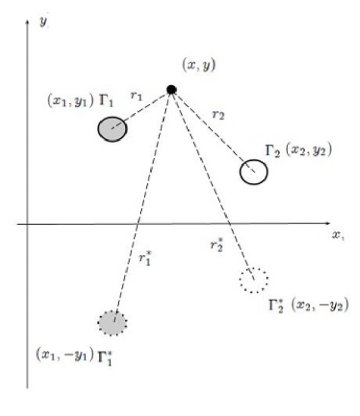
Figure 1. The basic geometry of vortices, image vortices and a tracer particle on the half plane

By superposition then, with arbitrary $\varpi_{1}=\Gamma_{1}$ $\delta(r_{1})$ and $\varpi_{2}=\Gamma_{2}\delta(r_{2})$ in layers 1 and 2 respectively the combined streamfunctions are

(9) $$\psi_{1}=\Gamma_{1}\left(\ln r_{1}-\ln r_{1}^{\ast}-K_{0}\left(r_{1}\right)+K_{0}\left(r_{1}^{\ast}\right)\right)+\Gamma_{2}\left(\ln r_{2}-\ln r_{2}^{\ast}+K_{0}\left(r_{2}\right)-K_{0}\left(r_{2}^{\ast}\right)\right)\text{,}\\ \psi_{2}=\Gamma_{2}\left(\ln r_{2}-\ln r_{2}^{\ast}-K_{0}\left(r_{2}\right)+K_{0}\left(r_{2}^{\ast}\right)\right)+\Gamma_{1}\left(\ln r_{1}-\ln r_{1}^{\ast}+K_{0}\left(r_{1}\right)-K_{0}\left(r_{1}^{\ast}\right)\right)\text{.}$$

Now the dynamics of the point vortices can be obtained by differentiation of the streamfunctions as follows

(10) $$\dot{x}_{i}=-\left.\frac{\partial\psi_{i}}{\partial y}\right|_{r=r_{i}},\text{ \ \ \ \ \ \ }\dot{y}_{i}=\left.\frac{\partial\psi_{i}}{\partial x}\right|_{r=r_{i}}\text{ \ \ }i=1,2\text{.}$$

It is well know that the equations for point vortices are a Hamiltonian system.  It can be verified that the energy of the system

(11) $${\displaystyle\int\limits_{H}}{\displaystyle\sum\limits_{i=1}^{2}}\left|\mathbf{v}_{i}\right|^{2}d\mathbf{x}\text{,}$$

is invariant. Integrating by parts, substituting for $\mathbf{v}_{i}$ using (10), $\psi_{i}$ using (9)and $\varpi_{1}$ using (2) as well as the $\ 0$ boundary conditions shows that the Hamiltonian can be simplified to,

(12) $$2H(\mathbf{\varpi})=-{\displaystyle\int\limits_{H}}\left(\psi_{1}\varpi_{1}+\psi_{2}\varpi_{2}\right)dxdy\text{,}$$

Using delta distributed point vortices $\varpi_{1}=\Gamma_{1}$ $\delta(r_{1})$and $\varpi_{2}=\Gamma_{2}\delta(r_{2})$ and the streamfunction for the ensemble (9) the invariant Hamiltonian for $\Gamma_{1}$ at $\left(x_{1},y_{1}\right)$ and $\Gamma_{2}$ at $\left(x_{2},y_{2}\right)$simplfies to

(13) $$H(\Gamma_{1},\Gamma_{2};\left(x_{1},y_{1}\right),\left(x_{2},y_{2}\right))=\\ \Gamma_{1}^{2}\left[K_{0}\left(r_{1,1^{\ast}}\right)-\ln r_{1,1^{\ast}}\right]+2\Gamma_{1}\Gamma_{2}\left[\ln r_{1,2}-\ln r_{1,2^{\ast}}+K_{0}\left(r_{1,2}\right)-K_{0}\left(r_{1,2^{\ast}}\right)\right]+\Gamma_{2}^{2}\left[K_{0}\left(r_{2,2^{\ast}}\right)-\ln r_{2,2^{\ast}}\right]\text{,}$$

again with reference to Fig.(1). Image vortices are denoted with a $\ast$. Note also from the symmetry of the geometry of Fig. (1) that $r_{1,2^{\ast}}=r_{2,1^{\ast}}$ and $r_{1,2}=r_{1^{\ast},2^{\ast}}$.

When $\Gamma_{2}=0$,   corresponding to a single vortex, the Hamiltonian, $H$ simplifies to $H=\Gamma_{1}^{2}\left[K_{0}\left(r_{1,1^{\ast}}\right)-\ln r_{1,1^{\ast}}\right]=C$ and by the monotonicity of $K_{0}\left(r_{1,1^{\ast}}\right)-\ln r_{1,1^{\ast}}$ we conclude that $r_{1,1^{\ast}}=constant$ corresponding to the vortex $\Gamma_{1}$ translating parallel to the $x$-axis.  This is the general solution then for the case of a single vortex. Notice also in (13) that the Hamiltonian,  $H$, is invariant with respect to arbitrary displacements of both $\Gamma_{1}$ at $\left(x_{1},y_{1}\right)$ and $\Gamma_{2}$ at $\left(x_{2},y_{2}\right)$ by $\delta$ in the $x$-direction. This implies by Noether’s theorem the invariance of

(14) $$\Gamma_{1}y_{1}+\Gamma_{2}y_{2}=c\text{.}$$

We provide an explicit proof of (14) in the appendix. The invariance of the Hamiltonian,  $H$, (13) and the momentum in the $y$-direction (14) imply that the 2 layer, 2 point vortex system in the half-plane is integrable. An easy way to see this is to notice that the Hamiltonian  depends only on $r_{1,1^{\ast}}=2y_{1}$ and $r_{2,2^{\ast}}=2y_{2}$ so that by (14) it depends only on either $y_{1}$ or $y_{2}$. The other term in the Hamiltonian is $r_{1,2}=\sqrt{\left(x_{1}-x_{2}\right)^{2}+\left(y_{1}-y_{2}\right)^{2}}$, from which we conclude that the Hamiltonian is a function of the two variables, $y_{1}$ (or $y_{2}$) and $\left|x_{1}-x_{2}\right|$.

3.
Characterizing 2 point vortex motion

We consider the cases $\Gamma_{1}=$ $\Gamma_{2}=1$ and $\Gamma_{1}=$ $-\Gamma_{2}=1$ separately.

3.1. The case $\Gamma_{1}=$ $-\Gamma_{2}=1$

In this case we use the invariant $\Gamma_{1}y_{1}+\Gamma_{2}y_{2}=c$ or $y_{1}-y_{2}=\alpha$ with parameter $\alpha$. With reference to Fig. (1)  we designate $y_{1}=y$ so that $y_{2}=y-\alpha$ (so that $y_{1}^{\ast}=-y$ and $y_{2}^{\ast}=\alpha-y$ and denote $x=\left|x_{1}-x_{2}\right|$ with the Hamiltonion (13) simplifying to

(15) $$H(x,y)=K_{0}\left(2y\right)+K_{0}\left(2\left(y-\alpha\right)\right)-\ln\left(2y\right)\left(2\left(y-\alpha\right)\right)\\ +\ln\frac{x^{2}+\left(2y-\alpha\right)^{2}}{x^{2}+\alpha^{2}}+2K_{0}\left(\sqrt{x^{2}+\left(2y-\alpha\right)^{2}}\right)-2K_{0}\left(\sqrt{x^{2}+\alpha^{2}}\right).$$

The Hamiltonian level curves are shown for various parameter values $\alpha$ in Fig. (2). There are no periodic solutions, and, in particular, no equilibria. We shall rigorously justifiy this in the sequel. There are two types of motion. The first corresponds to $\left|x_{1}-x_{2}\right|\rightarrow\infty$ and $y_{1}=y_{2}$ approaching a nonzero value, or vice versa $y_{1}=y_{2}\rightarrow\infty$ with $x=\left|x_{1}-x_{2}\right|$ approaching a nonzero value.  Which of these will depend on which side of the phase plane one begins; either on the front side or the back side of the phase plane. This is similar to the only type of motion seen for the one layer problem. See Fig (6) (a), for the corresponding case $y_{1}-y_{2}=\alpha=0$ for the one layer problem in the half plane. There is a second type of motion for the two layer problem seen, for all values of $\alpha$ including $\alpha=0$. These are phase curves that cross the $x=0$    or $\left|x_{1}-x_{2}\right|=0$ line. In the case that $\alpha=0$ this crossing corresponds to $\alpha=0=y_{1}-y_{2\text{ }}$ and $\left|x_{1}-x_{2}\right|=0$, which corresponds to vortex collapsing configurations. We are still investigating the nature of these collapsing configurations, as to whether they are finite time or infinite time vortex collapse solutions. Preliminary numerical results suggest that these are infinite time collapsing configurations. Notice that these collapsing configurations are not admitted for $\Gamma_{1}=$ $-\Gamma_{2}=1$, in the one layer case in the upper half plane.  See Fig (6) (a), for the corresponding case $y_{1}-y_{2}=\alpha=0$ for the one layer problem in the half plane and Fig (6) (b) for the case $y_{1}-y_{2}=\alpha=1$.  The second type of motion is seen in the one layer case, provide $\alpha>0$ such as $y_{1}-y_{2}=\alpha=1$, however while $\left|x_{1}-x_{2}\right|\rightarrow 0$, the $y$ values do not since $y_{1}-y_{2}=\alpha=1$.

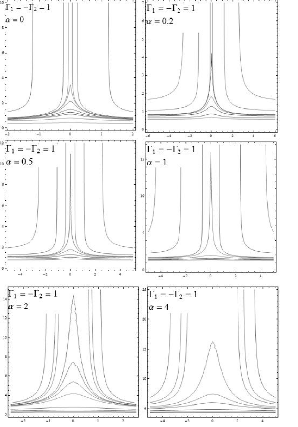
Figure 2. Hamiltonian level curves for $\Gamma_{1}=-\Gamma_{2}=1$, and parameter values $\alpha=0,0.2,0.5,1,2,4$.

3.2. The case $\Gamma_{1}=$ $\Gamma_{2}=1$

In this case we use the invariant $\Gamma_{1}y_{1}+\Gamma_{2}y_{2}=c$ or $y_{1}+y_{2}=\alpha$ with parameter $\alpha$. With reference to Fig. (1)  we designate $y_{1}=y$ so that $y_{2}=\alpha-y$ and denote $x=\left|x_{1}-x_{2}\right|$ with the Hamiltonian (13) simplifying to

(16) $$H(x,y)=K_{0}\left(2y\right)+K_{0}\left(2\left(\alpha-y\right)\right)-\ln\left(2y\right)\left(2\left(\alpha-y\right)\right)\\ +\ln\frac{x^{2}+\left(2y-\alpha\right)^{2}}{x^{2}+\alpha^{2}}+2K_{0}\left(\sqrt{x^{2}+\left(2y-\alpha\right)^{2}}\right)-2K_{0}\left(\sqrt{x^{2}+\alpha^{2}}\right).$$

The Hamiltonian level curves are shown for various parameter values $\alpha$ in Fig. (3). The motion in this case is very similar in many ways to the one layer problem with $\Gamma_{1}=$ $\Gamma_{2}=1$,(see Fig (6) (c)) with one minor difference.  The similarities include the two types of motions. Unlike the case $\Gamma_{1}=$ $\Gamma_{2}=-1$, the case $\Gamma_{1}=$ $\Gamma_{2}=1$ admits closed periodic solutions. Also in the two layer case the center of these periodic curves corresponds to a fixed equilibrium. As previously mentioned the two layer problem in the upper half plane for $\Gamma_{1}=$ $\Gamma_{2}=-1$ does not admit any equilibrium solutions. What is interesting about these fixed equilibria is that they are centered at $\left(x,y\right)=(0,\frac{\alpha}{2})$ corresponding to $x_{1}=x_{2\text{ }}$ and $y_{1}=y_{2}=\frac{\alpha}{2}$. The coordinates of both vortices are the same meaning they are stacked one on top of the other for the fixed equilibrium configuration.  We will study, more carefully, in what follows this equilibrium solution and rigorously show that there are no other equilibrium solutions for the case $\Gamma_{1}=$ $\Gamma_{2}=1$ in the upper half plane.

Clearly for the one layer problem we cannot have both $x_{1}=x_{2\text{ }}$and $y_{1}=y_{2}$ since there is freedom to stack the vortices, and so this would correspond to a collapsing configuration in which the vortices where initially located such that $x_{1}=x_{2\text{ }}$and $y_{1}=y_{2}$ which is not feasible. This is the one major difference between the two layer and one layer problems in the upper half plane for the case $\Gamma_{1}=$ $\Gamma_{2}=1$.

The second type of motion observed in Fig. (3), is a non periodic regime of motion in which either $\left|x_{1}-x_{2}\right|\rightarrow 0$ and $y_{1}$ approaches a nonzero number or where $\left|x_{1}-x_{2}\right|\rightarrow\infty$ and $y_{1}$ approaches a nonzero number. Which of these will again depend on which side of the phase plane one begins; either on the front side or the back side of the phase plane.

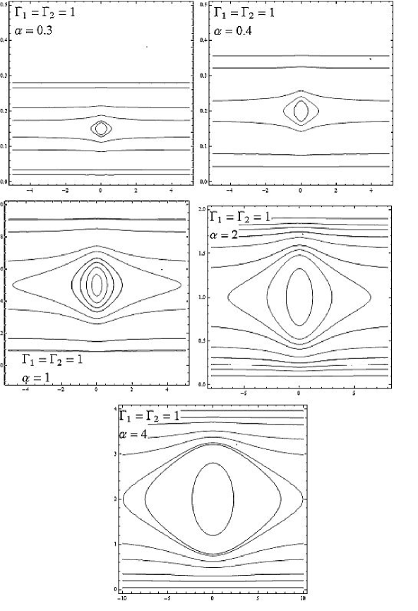
Figure 3. Hamiltonian level curves for $\Gamma_{1}=\Gamma_{2}=1$, and parameter values $\alpha=0,0.3,0.4,1,2,4$.

3.3. Equilibrium solutions

In this section we consider equilibrium solutions for the 2 vortex problem. We begin by showing that there are no relative equilibrium solutions when $\Gamma_{1}=$ $-\Gamma_{2}=1$ with vortex $1$, $\Gamma_{1}$ at $\left(x_{1},y_{1}\right)$ in layer $1$ and vortex $2$, $\Gamma_{2}$ at $\left(x_{2},y_{2}\right)=\left(x_{2},y_{1}-\alpha\right)$ in layer $2$. In this case the invariant $\Gamma_{1}y_{1}+\Gamma_{2}y_{2}=\alpha$, becomes $y_{1}-y_{2}=\alpha$. We consider the distance (see Fig. (4)) between the two vortices $\Gamma_{1}$ and $\Gamma_{2}$, $r_{1,2}(t)=\sqrt{\left(x_{1}-x_{2}\right)^{2}+\alpha^{2}}$ and show that it is never constant. Consider,

(17) $$\frac{dr_{1,2}^{2}}{dt}=\left(x_{1}-x_{2}\right)\left(\dot{x}_{1}-\dot{x}_{2}\right)+\left(y_{1}-y_{2}\right)\left(\dot{y}_{1}-\dot{y}_{2}\right)=\left(x_{1}-x_{2}\right)\left(\dot{x}_{1}-\dot{x}_{2}\right)+\left(y_{1}-y_{2}\right)(0)=\left(x_{1}-x_{2}\right)\left(\dot{x}_{1}-\dot{x}_{2}\right)\text{,}$$

where the last follows by the invariance of $y_{1}-y_{2}=\alpha$ or $\dot{y}_{1}-\dot{y}_{2}=0$. Using the equations (38,39) and $\Gamma_{1}=-$ $\Gamma_{2}=1$, we obtain,

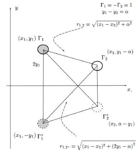
Figure 4. Two vortices in different layers $\Gamma_{1}=$ -$\Gamma_{2}=1$. In this case the invariant $\Gamma_{1}y_{1}+\Gamma_{2}y_{2}=\alpha$, becomes $y_{1}-y_{2}=\alpha$. $\Gamma_{1}$ in layer 1 at $\left(x_{1,}y_{1}\right)$, $\Gamma_{2}$ in layer 2 at $\left(x_{2,}y_{1}-\alpha\right)$ and $r_{1,2}=\sqrt{\left(x_{1}-x_{2}\right)^{2}+\alpha^{2}}$ and $r_{1,2^{\ast}}=\sqrt{\left(x_{1}-x_{2}\right)^{2}+\left(2y_{1}-\alpha\right)^{2}}$.

(18) $$\left(\dot{x}_{1}-\dot{x}_{2}\right)=K_{1}(2y_{1})+K_{1}(2y_{2})+\frac{2(y_{1}+y_{2})K_{1}(r_{1,2^{\ast}})}{r_{1,2^{\ast}}}+\frac{1}{2y_{1}}+\frac{1}{2y_{2}}-\frac{2(y_{1}+y_{2})}{r_{1,2^{\ast}}^{2}}>0\text{,}$$

where the inequality $\left(\dot{x}_{1}-\dot{x}_{2}\right)>0$ follows from the positivity $y_{1}>0,y_{2}>0,K_{1}(x)>0$ and the fact that

(19) $$\frac{1}{2y_{1}}+\frac{1}{2y_{2}}-\frac{2(y_{1}+y_{2})}{r_{1,2^{\ast}}^{2}}>0\text{,}$$

which can easily shown using the geometry of the upper half plane.

Next we show that there is only one relative equilibrium solutions when $\Gamma_{1}=$ $\Gamma_{2}=1$ with vortex $1$, $\Gamma_{1}$ at $\left(x_{1},y_{1}\right)$ in layer $1$ and vortex $2$, $\Gamma_{2}$ at $\left(x_{2},y_{2}\right)=\left(x_{2},\alpha-y_{1}\right)$ in layer $2$. This corresponds to the case $\left(x_{1,}y_{1}\right)=\left(x_{2,}y_{2}\right)$ corresponding to two vortices lying exactly one on top of the other.  Note this equilibrium position is not feasible in the one-layer case. These relative equilibria are clear in Fig. (3) in which $x=x_{1}-x_{2}=0$, and $y_{1}=y_{2}=\frac{\alpha}{2}$ and correspond to the center of the periodic orbits. In this case the invariant $\Gamma_{1}y_{1}+\Gamma_{2}y_{2}=\alpha$, becomes $y_{1}+y_{2}=\alpha$. We consider the distance (see Fig.(5)) between the two vortices $\Gamma_{1}$ and $\Gamma_{2}$, $r_{1,2}(t)=\sqrt{\left(x_{1}-x_{2}\right)^{2}+\left(2y_{1}-\alpha\right)^{2}}$ and show that it is never constant.

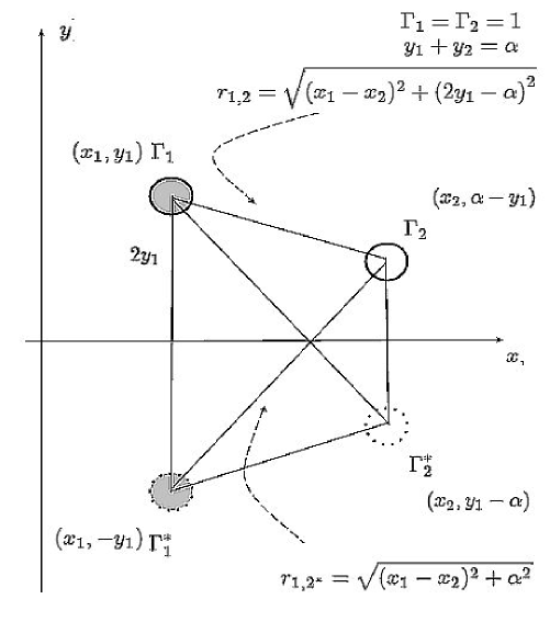
Figure 5. Two vortices in different layers $\Gamma_{1}=$ $\Gamma_{2}=1$. In this case the invariant $\Gamma_{1}y_{1}+\Gamma_{2}y_{2}=\alpha$, becomes $y_{1}+y_{2}=\alpha$. $\Gamma_{1}$ in layer 1 at $\left(x_{1,}y_{1}\right)$, $\Gamma_{2}$ in layer 2 at $\left(x_{2,}y_{1}-\alpha\right)$ and $r_{1,2}=\sqrt{\left(x_{1}-x_{2}\right)^{2}+\left(2y_{1}-\alpha\right)^{2}}$ and $r_{1,2^{\ast}}=\sqrt{\left(x_{1}-x_{2}\right)^{2}+\alpha^{2}}$.

Consider,

(20) $$\left(\dot{x}_{1}-\dot{x}_{2}\right)=K_{1}(2y_{1})-K_{1}(2y_{2})+\frac{2(y_{1}-y_{2})K_{1}(r_{1,2})}{r_{1,2}}+\frac{1}{2y_{1}}-\frac{1}{2y_{2}}-\frac{2(y_{1}-y_{2})}{r_{1,2}^{2}}\text{,}$$

(21) $$\dot{y}_{1}=\left(x_{1}-x_{2}\right)\left(\frac{K_{1}(r_{1,2^{\ast}})}{r_{1,2^{\ast}}}-\frac{K_{1}(r_{1,2})}{r_{1,2}}+\frac{1}{r_{1,2}^{2}}-\frac{1}{r_{1,2^{\ast}}^{2}}\right)\text{,}$$

(22) $$\frac{dr_{1,2}^{2}}{dt}=\left(x_{1}-x_{2}\right)\left(\dot{x}_{1}-\dot{x}_{2}\right)+\left(y_{1}-y_{2}\right)\left(\dot{y}_{1}-\dot{y}_{2}\right)=\\ \left(x_{1}-x_{2}\right)\left(K_{1}(2y_{1})-K_{1}(2y_{2})+\frac{2(y_{1}-y_{2})K_{1}(r_{1,2^{\ast}})}{r_{1,2^{\ast}}}+\frac{1}{2y_{1}}-\frac{1}{2y_{2}}-\frac{2(y_{1}-y_{2})}{r_{1,2^{\ast}}^{2}}\right)\text{.}$$

By considering the phase curves $\Gamma_{1}=$ $\Gamma_{2}=1$ shown in Fig. (3) we see that the curves all pass through $x=(x_{1}-x_{2})=0$.  We show that in this case $\left(\dot{x}_{1}-\dot{x}_{2}\right)\neq 0$ so that in Eq. (22) for a relative equilibrium

(23) $$K_{1}(2y_{1})-K_{1}(2y_{2})+\frac{2(y_{1}-y_{2})K_{1}(r_{1,2^{\ast}})}{r_{1,2^{\ast}}}+\frac{1}{2y_{1}}-\frac{1}{2y_{2}}-\frac{2(y_{1}-y_{2})}{r_{1,2^{\ast}}^{2}}=0\text{.}$$

Now when $x=x_{1}-x_{2}=0$, (20) becomes

(24) $$\left(\dot{x}_{1}-\dot{x}_{2}\right)=K_{1}(2y_{1})-K_{1}(2y_{2})+\frac{2(y_{1}-y_{2})K_{1}(\left|y_{1}-y_{2}\right|)}{\left|y_{1}-y_{2}\right|}+\frac{1}{2y_{1}}-\frac{1}{2y_{2}}-\frac{2(y_{1}-y_{2})}{\left|y_{1}-y_{2}\right|^{2}}\text{,}$$

which can be shown to be nonzero except when $y_{1}-y_{2}=0$ which would be simultaneous with $x_{1}-x_{2}=0$ So in Eq. (22) we require (23). In this case when $x_{1}-x_{2}=0$, (23) simplifies to

(25) $$K_{1}(2y_{1})-K_{1}(2y_{2})+\frac{2(y_{1}-y_{2})K_{1}(y_{1}+y_{2})}{r_{1,2^{\ast}}}+\frac{1}{2y_{1}}-\frac{1}{2y_{2}}-\frac{2(y_{1}-y_{2})}{(y_{1}+y_{2})^{2}}=0\text{,}$$

which again can be shown to be nonzero except when $y_{1}-y_{2}=0$ which would be simultaneous with $x_{1}-x_{2}=0$. The case $\Gamma_{1}=$ $\Gamma_{2}=1$ admits then the relative equilibria $\left(x_{1,}\frac{\alpha}{2}\right)=\left(x_{2,}\frac{\alpha}{2}\right)$ where the vortices lie exactly one on top of the other.  We can see that the phase curves (16) near this equilibrium position are closed periodic orbits so that the phase curves near to $\left(x_{1,}\frac{\alpha}{2}\right)=\left(x_{2,}\frac{\alpha}{2}\right)$ are almost relative equilibria, in the sense that the level curves (16) close to $\left(x_{1,}\frac{\alpha}{2}\right)=\left(x_{2,}\frac{\alpha}{2}\right)$ are asymptotically elliptical $\left(x_{1}-x_{2}\right)^{2}+(y_{1}-y_{2})^{2}=c^{2}$ or $\left(x_{1}-x_{2}\right)^{2}+(y_{1}-(\alpha-y_{1}))^{2}=c^{2}$ or $\left(x_{1}-x_{2}\right)^{2}+(2y_{1}-\alpha))^{2}=c^{2}$ corresponding to what would be a true relative equilibrium.

This is a novel relative equilibrium solution, keeping in mind that the one-layer two vortex problem on the upper half plan admits no relative equilibrium solutions.

3.4. Comparing with the one layer two vortex problem in the upper half plane

We summarize the one layer two vortex regimes of motion in the upper half plane for completeness and to highlight the similarities and differences we mentioned earlier.

In this case the Green’s functions using the method of images corresponds only to solving in one layer (2a) and not (2b) and is given by (3).  The general Hamiltonian becomes,

(26) $$H(\Gamma_{1},\Gamma_{2};\left(x_{1},y_{1}\right),\left(x_{2},y_{2}\right))=-\Gamma_{1}^{2}\ln r_{1,1^{\ast}}+2\Gamma_{1}\Gamma_{2}\ln\frac{r_{1,2}}{r_{1,2^{\ast}}}-\Gamma_{2}^{2}\ln r_{2,2^{\ast}}\text{.}$$

Again, use is made of the invariant $\Gamma_{1}y_{1}+$ $\Gamma_{2}y_{2}=\alpha$. We consider three representative cases:

1. $\Gamma_{1}=-\Gamma_{2}=1$ and $y_{1}-$ $y_{2}=\alpha=0.$ The Hamiltonian , using $x=\left|x_{1}-x_{2}\right|$ and $y_{1}=y_{2}=y$,

   (27) $$\frac{H(x,y)}{2}=\ln\frac{\sqrt{x^{2}+\left(2y\right)^{2}}}{2yx}\text{.}$$

2. $\Gamma_{1}=-\Gamma_{2}=1$ and $y_{1}-$ $y_{2}=\alpha=1$, so $y_{2}=y_{1}-\alpha=y-1$, with Hamiltonian

   (28) $$H(x,y)=-\ln(4y(y-1))+2\ln\frac{\sqrt{x^{2}+\left(2y-1\right)^{2}}}{\sqrt{x^{2}+1^{2}}}\text{.}$$

3. $\Gamma_{1}=\Gamma_{2}=1$ and $y_{1}+y_{2}=\alpha=1,$so $y_{2}=\alpha-y_{1}=1-y$, with Hamiltonian

   (29) $$H(x,y)=-\ln(4y(1-y))+2\ln\frac{\sqrt{x^{2}+\left(2y-1\right)^{2}}}{\sqrt{x^{2}+1^{2}}}\text{.}$$

   The phase curves are shown in Fig.(6) (a), (b) and (c) respectively.

   

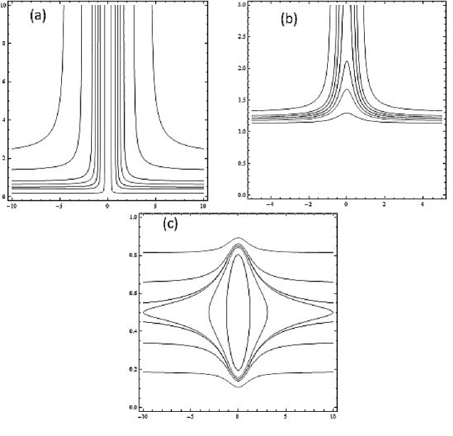
   Figure 6. Hamiltonian phase plots for the one layer two vortex problem (a)$\Gamma=-\Gamma_{2}=1$ and $y_{1}-$ $y_{2}=\alpha=0.$ (b)$\Gamma=-\Gamma_{2}=1$ and $y_{1}-$ $y_{2}=\alpha=1$, and (c) $\Gamma=\Gamma_{2}=1$ and $y_{1}+y_{2}=\alpha=1$.

   Notice, in particular, that when $\Gamma_{2}=0$   corresponding to a single vortex, the Hamiltonian, $H$ simplifies to $H=\Gamma_{1}^{2}\left[K_{0}\left(r_{1,1^{\ast}}\right)-\ln r_{1,1^{\ast}}\right]=C$ and by the monotonicity of $K_{0}\left(r_{1,1^{\ast}}\right)-\ln r_{1,1^{\ast}}$ we conclude that $r_{1,1^{\ast}}=constant$ corresponding to the vortex $\Gamma_{1}$ translating parallel to the $x$-axis.  This is the general solution then for the case of a single vortex. Notice also in (13) that the Hamiltonian,  $H$, is invariant with respect to arbitrary displacements of both $\Gamma_{1}$ at $\left(x_{1},y_{1}\right)$ and $\Gamma_{2}$ at $\left(x_{2},y_{2}\right)$ by $\delta$ in the $x$-direction. This implies by Noether’s theorem the invariance of

(30) $$\Gamma_{1}y_{1}+\Gamma_{2}y_{2}=c\text{.}$$

.

4.
Streamline topologies for the two vortex problem.

We consider the cases $\Gamma_{1}=$ $\Gamma_{2}=1$ and $\Gamma_{1}=$ $-\Gamma_{2}=1$ separately.

4.1. The case $\Gamma_{1}=$ $\Gamma_{2}=1$

We consider two basic configurations. One in which $\Gamma_{1}=$ $\Gamma_{2}=1$, with $\Gamma_{1}\$ in layer $1$, and $\Gamma_{2}\$ in layer $2$, with the same $y$-coordinate ($\beta$) as shown in Fig (7). We consider various values of the parameters $\alpha$ and $\beta$ with reference to Rossby radius of deformation $k=1$.

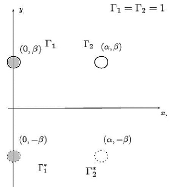
Figure 7. The configuration for streamline topologies with parameters $\alpha$, $\beta$. The streamline is $\psi_{1}=\ln\sqrt{x^{2}+(y-\beta)^{2}}-K_{0}\left(\sqrt{x^{2}+(y-\beta)^{2}}\right)+K_{0}\left(\sqrt{x^{2}+(y+\beta)^{2}}\right)-\ln\sqrt{x^{2}+(y+\beta)^{2}}+\ln\sqrt{(x-\alpha)^{2}+(y-\beta)^{2}}+K_{0}\left(\sqrt{(x-\alpha)^{2}+(y-\beta)^{2}}\right)-K_{0}\left(\sqrt{(x-\alpha)^{2}+(y+\beta)^{2}}\right)-\ln\left(\sqrt{(x-\alpha)^{2}+(y+\beta)^{2}}\right)$

The streamlines are shown in Fig. (8) for this case with $\beta=0.5$ and in Fig. (9) for the case $\beta=2$. For the case $\beta=0.5$ the streamlines are topologically similar as $\alpha$ is varied. For the case $\beta=2$ the streamlines undergo topological change as $\alpha$ changes through $\alpha=3$ to $\alpha=5$ with the introduction of a saddle stagnation point.

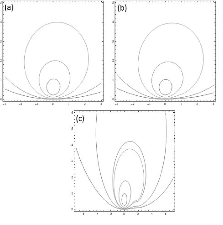
Figure 8. Streamlines for horizontal configurations. $\Gamma_{1}=\Gamma_{2}$ in layers $1$ and $2$ respectively. $\beta=0.5$. (a) $\alpha=0.6$, (b) $\alpha=1$, and (c) $\alpha=2$.

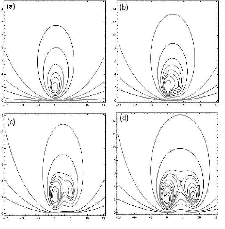
Figure 9. Streamlines for horizontal configurations. $\Gamma_{1}=\Gamma_{2}$ in layers $1$ and $2$ respectively. $\beta=2$. (a) $\alpha=0.6$, (b) $\alpha=3$, (c) $\alpha=5$ and (d) $\alpha=8$

The second basic configuration we consider is with 2 vortices placed in a vertical configuration, with $\Gamma_{1}$ in layer $1$ and $\Gamma_{2}$ in layer $2$ as shown in Fig. (10). In this case $x_{1}=x_{2}=0$.

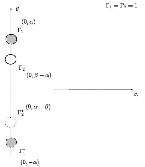
Figure 10. The configuration for streamline topologies with parameters $\alpha$, $\beta$. Here $\Gamma_{1}$ is at $\left(0,\alpha\right)$, and $\Gamma_{2}$ is at $\left(0,\beta-\alpha\right)$ and $y_{1}+y_{2}=\beta$ is invariant. The streamline is $\psi_{1}=\ln\sqrt{x^{2}+(y-\alpha)^{2}}-K_{0}\left(\sqrt{x^{2}+(y-\alpha)^{2}}\right)+K_{0}\left(\sqrt{x^{2}+(y+\alpha)^{2}}\right)-\ln\sqrt{x^{2}+(y+\alpha)^{2}}+\ln\sqrt{x^{2}+(y+\alpha-\beta)^{2}}+K_{0}\left(\sqrt{x^{2}+(y+\alpha-\beta)^{2}}\right)-K_{0}\left(\sqrt{x^{2}+(y+\beta-\alpha)^{2}}\right)-\ln\left(\sqrt{x^{2}+(y+\beta-\alpha)^{2}}\right)$

In this case 3 classes of streamlines are observed. Notice that $\alpha<\beta$, and $y_{1}+y_{2}=\beta$ is invariant. The first streamline case corresponds to when $\alpha<<\beta$ (when $\Gamma_{1}$ and $\Gamma_{2\text{ }}$are relatively far apart) and is shown in Fig. (11(a)). There is a saddle stagnation point observed for this case. The second case corresponds to when $\alpha\approx\beta$ (so that is close to the boundary) and is shown in Fig. (11(b)). The third case corresponds to the intermediate case when $\alpha$ is not much smaller than $\beta$ but not too similar in magnitute to  $\beta$ either and is depicted in Fig. (11(c)). For the cases $\alpha\approx\beta$ and the intermediate case when $\alpha$ is not much smaller than $\beta$ but not too similar in magnitute to  $\beta$ there are no stagnation points.  While in both of these cases the streamlines are in many ways topologically similar, the two layer interaction does introduce distortion effects upon a closer examination of (11(b)) and (11(c)).

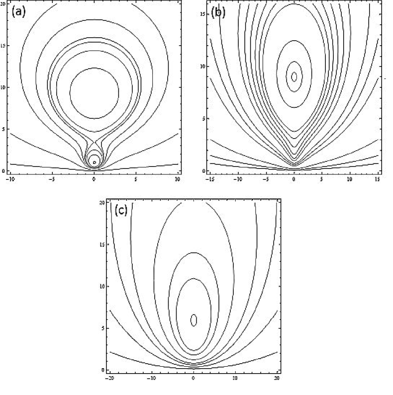
Figure 11. Streamlines for vertical configurations. $\Gamma_{1}=\Gamma_{2}$ in layers $1$ and $2$ respectively with $\Gamma_{1}$ at $\left(0,\alpha\right)$ and $\Gamma_{2}$ at $\left(0,\beta-\alpha\right)$. In this case $y_{1}+y_{2}=\beta$. (a) $\alpha<<\beta$; observed for $\left(\alpha,\beta\right)=\left(0.1,2\right);\left(\alpha,\beta\right)=\left(1,10\right);\left(\alpha,\beta\right)=\left(25,30\right)$ (b) $\alpha\approx\beta,$ observed for $\left(\alpha,\beta\right)=\left(9,10\right);\left(\alpha,\beta\right)=\left(29,30\right)$ (c) $\alpha$ not much smaller than $\beta$ but not too close in magnitude to $\beta$ either, observed for $\left(\alpha,\beta\right)=\left(0.5,1\right);\left(\alpha,\beta\right)=\left(1,2\right);\left(\alpha,\beta\right)=\left(6,10\right);$

4.2. The case $\Gamma_{1}=-$ $\Gamma_{2}=1$

We consider the same two basic configurations. One in which $\Gamma_{1}=$ $-\Gamma_{2}=1$, with $\Gamma_{1}\$ in layer $1$, and $\Gamma_{2}\$ in layer $2$, with the same $y$-coordinate as shown in Fig (7). We consider various values of the parameters $\alpha$ and $\beta$ with reference to Rossby radius of deformation $k=1$. Note in this case $\Gamma_{1}y_{1}+\Gamma_{2}y_{2}=y_{1}-y_{2}=0$ is invariant.  The streamlines are shown for $\beta=2$ in Fig (12).  For all values of $\beta$ (including $\beta=0.5;2;10$) a stagnation streamline emanating from the bounary is observed. There is a stagnation point at the boundary from which the stagnation streamline originates. As seen for the case $\beta=2$ in Fig (12) the basic topology of the streamline does not change as $\alpha$ is varied from $\alpha=0.1$ through $\alpha=10$.

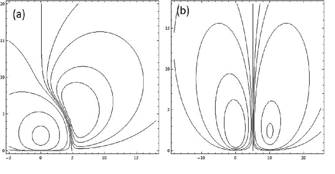
Figure 12. Streamlines for $\Gamma_{1\text{ }}$in layer 1 at $\left(0,\beta\right)$, $\Gamma_{2\text{ }}$in layer 2 at $\left(\alpha,\beta\right)$.In this case $y_{1}-y_{2}=0$ is invariant. (a) $\beta=2;\alpha=0.1$ and (b)$\beta=2;\alpha=10$. The streamfunction is $\psi_{1}=\ln\sqrt{x^{2}+(y-\beta)^{2}}-K_{0}\left(\sqrt{x^{2}+(y-\beta)^{2}}\right)+K_{0}\left(\sqrt{x^{2}+(y+\beta)^{2}}\right)-\ln\sqrt{x^{2}+(y+\beta)^{2}}-\ln\sqrt{\left(x-\alpha\right)^{2}+(y-\beta)^{2}}-K_{0}\left(\sqrt{\left(x-\alpha\right)^{2}+(y-\beta)^{2}}\right)+K_{0}\left(\sqrt{\left(x-\alpha\right)^{2}+(y+\beta)^{2}}\right)+\ln\left(\sqrt{\left(x-\alpha\right)^{2}+(y+\beta)^{2}}\right)$

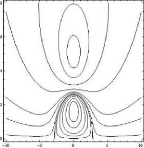
Figure 13. Streamlines for $\Gamma_{1\text{ }}$in layer 1 at $\left(0,\alpha\right)$, $\Gamma_{2\text{ }}$in layer 2 at $\left(0,\alpha-\beta\right)$.In this case $y_{1}-y_{2}=\beta$ is invariant. The typical case $\beta=3;\alpha=5$ is shown. The streamfunction is $\psi_{1}=\ln\sqrt{x^{2}+(y-\alpha)^{2}}-K_{0}\left(\sqrt{x^{2}+(y-\alpha)^{2}}\right)+K_{0}\left(\sqrt{x^{2}+(y+\alpha)^{2}}\right)-\ln\sqrt{x^{2}+(y+\alpha)^{2}}-\ln\sqrt{x^{2}+(y-\left(\alpha-\beta\right))^{2}}-K_{0}\left(\sqrt{x^{2}+(y-\left(\alpha-\beta\right))^{2}}\right)+K_{0}\left(\sqrt{x^{2}+(y+\left(\alpha-\beta\right))^{2}}\right)+\ln\left(\sqrt{x^{2}+(y+\left(\alpha-\beta\right))^{2}}\right)$

The second configuration is as before with $\Gamma_{1}=$ $-\Gamma_{2}=1$, with $\Gamma_{1}\$ in layer $1$ and $\Gamma_{2}\$ in layer $2$ . The 2 vortices are placed in a vertical configuration, with $\Gamma_{1}$ in layer $1$ at $\left(0,\alpha\right)$ and $\Gamma_{2}$ in layer $2$ at $\left(0,\alpha-\beta\right)$ shown in Fig. (10). In this case $x_{1}=x_{2}=0$. We consider various values of the parameters $\alpha$ and $\beta$ with reference to Rossby radius of deformation $k=1$. Note in this case $\Gamma_{1}y_{1}+\Gamma_{2}y_{2}=y_{1}-y_{2}=\beta$ is invariant.  In this case there is a stagnation streamline joining two stagnation points on the boundary as seen in Fig. (13).

5. Integrable 3 vortex configurations–Relative equilibria.

We conclude with a Hamiltonian study of integrable two-layer 3 vortex motion on the half plane by studying integrable symmetrical configurations and provide a rich class of new relative equilibria. We consider two basic symmetrical configurations of 3 vortices as depicted in Fig.(14). We seek relative equilibrium solutions.in which the initial configuration is rigidly maintained.  The method we adopt is similar to that as in the work of Jamaloodeen and Newton [8] in which we seek relative equilbria base on a a symmetrical configuration and vary parameters that ensure the relative equilbrium or rigid shape is invariant.

5.1. The case $\Gamma_{1}=$ $\Gamma_{2}=1,\Gamma_{3}=-\alpha$ with $\Gamma_{1}$ at $\left(x,y\right)$, $\Gamma_{2}$ at $\left(-x,y\right)$ (in layer 1) and $\Gamma_{3}$ at $\left(0,y_{3}\right)$ (in layer 2)

In the first symmetrical configuration we have $\Gamma_{1}=$ $\Gamma_{2}=1$, with $\Gamma_{1}\$ in layer $1$, and $\Gamma_{2}\$ in layer $2$, with the same $y$-coordinate as shown in Fig (14)(a). In this case it can be shown that $\dot{x}_{1}=\dot{x}_{2}$ and $\dot{y}_{1}=-\dot{y}_{2}$. The invariant $\Gamma_{1}y_{1}+\Gamma_{2}y_{2}+\Gamma_{3}y_{3}=\beta$, becomes $y_{1}+y_{2}-\alpha y_{3}=\beta$, or $y_{3}=\frac{y_{1}+y_{2}-\beta}{\alpha}$. Relative equilibrium solutions will then be admitted, for this configuration, by requiring that $\dot{y}_{1}=0$, and $\dot{x}_{1}=\dot{x}_{3}$. These equations (see Appendix B for their explicit forms) are solved numerically with $\alpha$ and $\beta$ considered as parameters. These are summarized in in Tables (31)-(32), and exploiting the symmetry and the invariant $y_{1}+y_{2}-\alpha y_{3}=\beta$, or $y_{3}=\frac{y_{1}+y_{2}-\beta}{\alpha},$ only the coordinates $\left(x_{1},y_{1}\right)=\left(x,y\right)$ are given.

Figure 14. Integrable 3 vortex relative equilibrium solutions depending on parameters, $\alpha$, and $\beta$. The invariant $\Gamma_{1}y_{1}+\Gamma_{2}y_{2}+\Gamma_{3}y_{3}=\beta$ becomes $y_{1}+y_{2}-\alpha y_{3}=\beta$ with $\Gamma_{1}=\Gamma_{2}=1$, $\Gamma_{3}=-\alpha$, so that $y_{3}=\frac{y_{1}+y_{2}-\beta}{\alpha}$. $\Gamma_{1}$ and $\Gamma_{2}$ are in layer 1, $\Gamma_{3}$ is in layer 2. In (a) $\Gamma_{1}$ and $\Gamma_{2}$ are placed at $\left(x,y\right)$ and $\left(-x,y\right)$ respectively. In (b) $\Gamma_{1}$ and $\Gamma_{2}$ are placed at $\left(0,y_{1}\right)$ and $\left(0,y_{2}\right)$ respectively.

(31)

$$\left(\alpha,\beta\right)$$ (negative Relative equilibrium

(32)

$$\left(\alpha,\beta\right)$$ (positive Relative equilibrium

  

Notice that the numerical evidence suggest that there are no relative equilibria corresponding to this configuration with $\alpha$ negative or $\Gamma_{3}>0$. There also appears to be a complicated bifurcation of these relative equilibria. For example fixing $\beta$ and varying $\alpha$ gives varying numbers of relative equilibria. Consider, for example the case $\beta=-0.75$ for which at $\alpha=2.01$, there is one relative equilibrium solution, then increasing $\alpha$ through $\alpha=2.09$ there are two and likewise two, again, after increasing $\alpha$ through $\alpha=2.15$ and finally increasing $\alpha$ to $\alpha=2.19$ there is again only one relative equilibrium solution. Similarly when $\beta=0.5$ there is one equilibrium configuration when $\alpha=1.888$, two equilibrium configurations when $\alpha=1.9$ and three equilibrium configurations when $\alpha$ increases through $\alpha=1.95$. A scatterplot of all numerically found relative equilibria from Tables (31)-(32) is shown in Fig(15), with associated $\left(\alpha,\beta\right)$ for each configuration $\left(x_{1},y_{1}\right)=\left(x,y\right)$ suppressed.

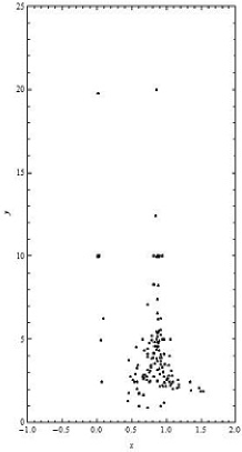
Figure 15. A scatterplot of all numerically found relative equilibria from Tables (31)-(32) with associated $\left(\alpha,\beta\right)$ for each configuration $\left(x_{1},y_{1}\right)=\left(x,y\right)$ suppressed.

It is also possible that some of these relative equilibria are fixed equilibria, meaning that in fact not only are $\dot{y}_{1}=0$, and $\dot{x}_{1}=\dot{x}_{3}$ but $\dot{y}_{1}=0$, and $\dot{x}_{1}=\dot{x}_{3}=0$. However preliminary numerical studies suggest that there are no fixed equilibrium configurations of the kind depicted in Fig(14)(a).  The bifurcation sequence suggested above and the fixed equilibria are topics for further study.

5.2. The case $\Gamma_{1}=$ $\Gamma_{2}=1,\Gamma_{3}=-\alpha$ with $\Gamma_{1}$ at $\left(0,y_{1}\right)$, $\Gamma_{2}$ at $\left(0,y_{2}\right)$ (in layer 1) and $\Gamma_{3}$ at $\left(0,y_{3}\right)$ (in layer 2)

In the second symmetrical configuration we have $\Gamma_{1}=$ $\Gamma_{2}=1$, with $\Gamma_{1}\$ in layer $1$, and $\Gamma_{2}\$ in layer $2$, with $\Gamma_{1}$ at $\left(0,y_{1}\right)$, $\Gamma_{2}$ at $\left(0,y_{2}\right)$ (in layer 1) and $\Gamma_{3}$ at $\left(0,y_{3}\right)$ (in layer 2)with the same $y$-coordinate as shown in Fig (14)(b). In this case it can be shown that $\dot{x}_{1}=\dot{x}_{2}$ and $\dot{y}_{1}=-\dot{y}_{2}$. The invariant $\Gamma_{1}y_{1}+\Gamma_{2}y_{2}+\Gamma_{3}y_{3}=\beta$, becomes $y_{1}+y_{2}-\alpha y_{3}=\beta$, or $y_{3}=\frac{y_{1}+y_{2}-\beta}{\alpha}$. In this case it can be shown that $\dot{y}_{1}=\dot{y}_{2}=\dot{y}_{3}=0$. Relative equilibrium solutions will then be admitted, for this configuration by requiring that $\dot{x}_{1}=\dot{x}_{2}=\dot{x}_{3}$. Again the invariant $\Gamma_{1}y_{1}+\Gamma_{2}y_{2}+\Gamma_{3}y_{3}=\beta$, becomes $y_{1}+y_{2}-\alpha y_{3}=\beta$, or $y_{3}=\frac{y_{1}+y_{2}-\beta}{\alpha}$. These equations (see Appendix B for their explicit forms) are solved numerically with $\alpha$ and $\beta$ considered as parameters. These are summarized in in Tables (33)-(34), and exploiting the symmetry and the invariant $y_{1}+y_{2}-\alpha y_{3}=\beta$, or $y_{3}=\frac{y_{1}+y_{2}-\beta}{\alpha},$ again it suffices to provide only the coordinates for $\left(y_{1},y_{2}\right)=(Y,y)$.

(33)

$$\left(\alpha,\beta\right)$$ () Relative equilibrium

No numerical relative equilibrium configurations

    

(34)

$$\left(\alpha,\beta\right)$$ () Relative equilibrium

      

Notice again that the numerical evidence suggests that there are no relative equilibria corresponding to this configuration with $\alpha$ negative or $\Gamma_{3}>0$. There again appears to be a complicated bifurcation of these relative equilibria. For example fixing $\alpha$ and varying $\beta$ gives varying numbers of relative equilibria. A scatterplot of all numerically found relative equilibria from Tables (33)-(34) is shown in Fig(15), with associated $\left(\alpha,\beta\right)$ for each configuration $\left(0,y_{1}\right)=\left(0,Y\right)\$and $\left(0,y_{2}\right)=\left(0,y\right)$ suppressed.

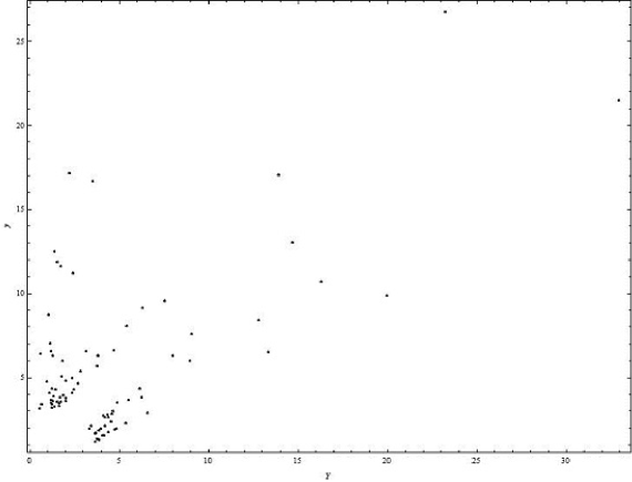
Figure 16. A scatterplot of all numerically found relative equilibria from Tables (33)-(34) with associated $\left(\alpha,\beta\right)$ for each configuration $\left(0,y_{1}\right)=\left(0,Y\right)\$and $\left(0,y_{2}\right)=\left(0,y\right)$ or $\left(Y,y\right)$ suppressed.

6.
Conclusion

We have presented results on integrable two-layer point vortex motion on the upper half plane and shown similarities and differences with integrable  one-layer point vortex motion in the upper half plane and with integrable two-layer point vortex motion on the entire plane including the study of equilbrium solutions, the finite-time vortex collapse problem and a study of streamline topologies.  At present we are also pursuing work to determine 3 or 4 vortex initial vortex configurations that lead to finite time collapse of the vortices. Should such configurations exist, they will depend on the initial configuration of the vortices and the vortex strengths, and would possibly be self-similar. Also of interest would be to perform a systematic bifurcation analysis of the 3 vortex relative equilibria we found shown in Figs.(15-16). The bifurcation analysis in both cases would depend on the parameter $\left(\alpha,\beta\right)$ as depicted in Fig. (14). Finally we are also pursuing work in the direction of establishing conditions under which 3 vortices may induce chaotic advection of fluid particles much along the lines for the two layer problem in the entire plane as done in the work of Koshel et al[11]. A good starting point are perturbations of the configurations used to obtain the streamlines depicted in Figs. (7 and 10).

Appendix A Explicit proof that $\sum\Gamma_{i}=c$ is invariant

We show that $\Gamma_{1}\dot{y}_{1}+\Gamma_{2}\dot{y}_{2}=0$. Use,

(35) $$\dot{x}_{i}=-\left.\frac{\partial\psi_{i}}{\partial y}\right|_{\left(x_{i},y_{i}\right)},\text{ \ \ \ \ \ \ }\dot{y}_{i}=\left.\frac{\partial\psi_{i}}{\partial x}\right|_{{}_{\left(x_{i},y_{i}\right)}}\text{ \ }$$

(36) $$\text{\ }\dot{y}_{1}=\left.\frac{\partial\psi_{1}}{\partial x}\right|_{{}_{\left(x_{1},y_{1}\right)}}=\Gamma_{1}\left(-K_{1}\left(2y_{1}\right)\right)\frac{2\left(x_{1}-x_{1}\right)}{2r_{1,1^{\ast}}}-\frac{\Gamma_{1}}{2r_{1,1^{\ast}}^{2}}2\left(x_{1}-x_{1}\right)+\frac{\Gamma_{2}}{2r_{1,2}^{2}}2\left(x_{1}-x_{2}\right)\\ -\Gamma_{2}K_{1}\left(r_{1,2}\right)\frac{2\left(x_{1}-x_{2}\right)}{2r_{1,2}}+\Gamma_{2}K_{1}\left(r_{1,2^{\ast}}\right)\frac{2\left(x_{1}-x_{2}\right)}{2r_{1,2^{\ast}}}-\frac{\Gamma_{2}}{2r_{1,2^{\ast}}^{2}}2\left(x_{1}-x_{2}\right)\\ =\Gamma_{2}\left(x_{1}-x_{2}\right)\left[\frac{1}{r_{1,2}^{2}}-\frac{K_{1}\left(r_{1,2}\right)}{r_{1,2}}+\frac{K_{1}\left(r_{1,2^{\ast}}\right)}{r_{1,2^{\ast}}}-\frac{1}{r_{1,2^{\ast}}^{2}}\right]$$

(37) $$\text{\ }\dot{y}_{2}=\left.\frac{\partial\psi_{1}}{\partial x}\right|_{{}_{\left(x_{2},y_{2}\right)}}=\Gamma_{1}K_{1}\left(2y_{1}\right)\frac{2\left(x_{2}-x_{2}\right)}{2r_{2,2^{\ast}}}-\frac{\Gamma_{2}}{2r_{2,2^{\ast}}^{2}}2\left(x_{2}-x_{2}\right)+\frac{\Gamma_{1}}{2r_{1,1}^{2}}2\left(x_{2}-x_{1}\right)\\ -\Gamma_{1}K_{1}\left(r_{2,1}\right)\frac{2\left(x_{2}-x_{1}\right)}{2r_{2,1}}+\Gamma_{1}K_{1}\left(r_{2,1^{\ast}}\right)\frac{2\left(x_{2}-x_{1}\right)}{2r_{2,1^{\ast}}}-\frac{\Gamma_{1}}{2r_{2,1^{\ast}}^{2}}2\left(x_{2}-x_{1}\right)\\ =\Gamma_{1}\left(x_{2}-x_{1}\right)\left[\frac{1}{r_{2,1}^{2}}-\frac{K_{1}\left(r_{2,1}\right)}{r_{2,1}}+\frac{K_{1}\left(r_{2,1^{\ast}}\right)}{r_{2,1^{\ast}}}-\frac{1}{r_{2,1^{\ast}}^{2}}\right]\text{.}$$

Here $K_{0}^{{}^{\prime}}(r)=-K_{1}\left(r\right)$ It is clear that since $r_{2,1}=r_{2,1}$ and $r_{1,2^{\ast}}=r_{2,1^{\ast}}$ that $\Gamma_{1}\dot{y}_{1}+\Gamma_{2}\dot{y}_{2}=0$.

For completeness we present the dynamical equations for the $x$-components, for reference as needed when used.

(38) $$\dot{x}_{1}=-\left.\frac{\partial\psi_{1}}{\partial y}\right|_{{}_{\left(x_{2},y_{2}\right)}}=\Gamma_{1}\left[K_{1}\left(2y_{1}\right)+\frac{1}{2y_{1}}\right]\ +\frac{\Gamma_{2}\left(y_{1}-y_{2}\right)}{r_{1,2}}\left[K_{1}\left(r_{1,2}\right)-\frac{1}{r_{1,2}}\right]\\ +\frac{\Gamma_{2}\left(y_{1}+y_{2}\right)}{r_{1,2^{\ast}}}\left[\frac{1}{r_{1,2^{\ast}}}-K_{1}\left(r_{1,2^{\ast}}\right)\right]\text{.}$$

(39) $$\dot{x}_{2}=-\left.\frac{\partial\psi_{2}}{\partial y}\right|_{{}_{\left(x_{2},y_{2}\right)}}=\Gamma_{1}\left[K_{1}\left(2y_{2}\right)+\frac{1}{2y_{2}}\ \right]+\frac{\Gamma_{2}\left(y_{2}-y_{1}\right)}{r_{1,2}}\left[K_{1}\left(r_{1,2}\right)-\frac{1}{r_{1,2}}\right]\\ +\frac{\Gamma_{2}\left(y_{1}+y_{2}\right)}{r_{1,2^{\ast}}}\left[\frac{1}{r_{1,2^{\ast}}}-K_{1}\left(r_{1,2^{\ast}}\right)\right]\text{.}$$

Appendix B Equations of motion for symmetric integrable 3 vortex configurations

We provide the equations of motion for the two cases considered.

B.1. The case $\Gamma_{1}=$ $\Gamma_{2}=1,\Gamma_{3}=-\alpha$ with $\Gamma_{1}$ at $\left(x,y\right)$, $\Gamma_{2}$ at $\left(-x,y\right)$ (in layer 1) and $\Gamma_{3}$ at $\left(0,y_{3}\right)$ (in layer 2)

In this case it can be shown that $\dot{x}_{1}=\dot{x}_{2}$ and $\dot{y}_{1}=-\dot{y}_{2}$. Relative equilibrium solutions will then be admitted, for this configuration by requiring that $\dot{y}_{1}=0$, and $\dot{x}_{1}=\dot{x}_{3}$. In this case the invariant $\Gamma_{1}y_{1}+\Gamma_{2}y_{2}+\Gamma_{3}y_{3}=\beta$, becomes $y_{1}+y_{2}-\alpha y_{3}=\beta$, or $y_{3}=\frac{y_{1}+y_{2}-\beta}{\alpha}$.

$$\dot{y}_{1} =\frac{1\text{\ }}{2x}+K_{1}\left(2x\right)-\frac{2x}{\left(2x\right)^{2}+\left(2y\right)^{2}}-\frac{2xK_{1}\left(\sqrt{\left(2x\right)^{2}+\left(2y\right)^{2}}\right)}{\sqrt{\left(2x\right)^{2}+\left(2y\right)^{2}}}$$

$$-\frac{\alpha x}{x^{2}+\left(y-y_{3}\right)^{2}}+\frac{\alpha xK_{1}\left(\sqrt{x^{2}+\left(y-y_{3}\right)^{2}}\right)}{\sqrt{x^{2}+\left(y-y_{3}\right)^{2}}}$$

(40) $$+\frac{\alpha x}{x^{2}+\left(y+y_{3}\right)^{2}}-\frac{\alpha xK_{1}\left(\sqrt{x^{2}+\left(y+y_{3}\right)^{2}}\right)}{\sqrt{x^{2}+\left(y+y_{3}\right)^{2}}}$$

$$\dot{x}_{1} =-\frac{1\text{\ }}{2y}-K_{1}\left(2y\right)-\frac{2y}{\left(2x\right)^{2}+\left(2y\right)^{2}}-\frac{2yK_{1}\left(\sqrt{\left(2x\right)^{2}+\left(2y\right)^{2}}\right)}{\sqrt{\left(2x\right)^{2}+\left(2y\right)^{2}}}$$

$$-\frac{\alpha\left(y-y_{3}\right)}{x^{2}+\left(y-y_{3}\right)^{2}}+\frac{\alpha\left(y-y_{3}\right)K_{1}\left(\sqrt{x^{2}+\left(y-y_{3}\right)^{2}}\right)}{\sqrt{x^{2}+\left(y-y_{3}\right)^{2}}}$$

(41) $$+\frac{\alpha\left(y+y_{3}\right)}{x^{2}+\left(y+y_{3}\right)^{2}}-\frac{\alpha\left(y+y_{3}\right)K_{1}\left(\sqrt{x^{2}+\left(y+y_{3}\right)^{2}}\right)}{\sqrt{x^{2}+\left(y+y_{3}\right)^{2}}}$$

$$\dot{x}_{3} =\frac{\alpha\text{\ }}{2y_{3}}+\alpha K_{1}\left(2y_{3}\right)+\frac{2\left(y_{3}-y\right)}{x^{2}+\left(y_{3}-y\right)^{2}}-\frac{2\left(y_{3}-y\right)K_{1}\left(\sqrt{x^{2}+\left(y_{3}-y\right)^{2}}\right)}{\sqrt{x^{2}+\left(y_{3}-y\right)^{2}}}$$

(42) $$-\frac{2\left(y_{3}+y\right)}{x^{2}+\left(y_{3}+y\right)^{2}}-\frac{2\left(y_{3}+y\right)K_{1}\left(\sqrt{x^{2}+\left(y_{3}+y\right)^{2}}\right)}{\sqrt{x^{2}+\left(y_{3}+y\right)^{2}}}$$

B.2. The case $\Gamma_{1}=$ $\Gamma_{2}=1,\Gamma_{3}=-\alpha$ with $\Gamma_{1}$ at $\left(0,y_{1}\right)$, $\Gamma_{2}$ at $\left(0,y_{2}\right)$ (in layer 1) and $\Gamma_{3}$ at $\left(0,y_{3}\right)$ (in layer 2)

In this case it can be shown that $\dot{y}_{1}=\dot{y}_{2}=\dot{y}_{3}=0$. Relative equilibrium solutions will then be admitted, for this configuration by requiring that $\dot{x}_{1}=\dot{x}_{2}=\dot{x}_{3}$. Again the invariant $\Gamma_{1}y_{1}+\Gamma_{2}y_{2}+\Gamma_{3}y_{3}=\beta$, becomes $y_{1}+y_{2}-\alpha y_{3}=\beta$, or $y_{3}=\frac{y_{1}+y_{2}-\beta}{\alpha}$.

$$\dot{x}_{1} =-\frac{1\text{\ }}{2y_{1}}-K_{1}\left(2y_{1}\right)+\frac{\left(y_{1}-y_{2}\right)}{\left|y_{1}-y_{2}\right|^{2}}+\frac{\left(y_{1}-y_{2}\right)K_{1}\left(\left|y_{1}-y_{2}\right|\right)}{\left|y_{1}-y_{2}\right|}$$

$$-\frac{1}{y_{1}+y_{2}}-K_{1}\left(y_{1}+y_{2}\right)$$

(43) $$- \frac{\alpha\left(y_{1}-y_{3}\right)}{\left|y_{1}-y_{3}\right|^{2}}+\frac{\alpha\left(y_{1}-y_{3}\right)K_{1}\left(\left|y_{1}-y_{3}\right|\right)}{\left|y_{1}-y_{3}\right|}+\frac{\alpha}{y_{1}+y_{3}}-\alpha K_{1}\left(y_{1}+y_{3}\right)$$

$$\dot{x}_{2} =-\frac{1\text{\ }}{2y_{2}}-K_{1}\left(2y_{2}\right)+\frac{\left(y_{2}-y_{1}\right)}{\left|y_{2}-y_{1}\right|^{2}}+\frac{\left(y_{2}-y_{1}\right)K_{1}\left(\left|y_{2}-y_{1}\right|\right)}{\left|y_{2}-y_{1}\right|}$$

$$-\frac{1}{y_{1}+y_{2}}-K_{1}\left(y_{1}+y_{2}\right)$$

(44) $$- \frac{\alpha\left(y_{2}-y_{3}\right)}{\left|y_{2}-y_{3}\right|^{2}}+\frac{\alpha\left(y_{2}-y_{3}\right)K_{1}\left(\left|y_{2}-y_{3}\right|\right)}{\left|y_{2}-y_{3}\right|}+\frac{\alpha}{y_{2}+y_{3}}-\alpha K_{1}\left(y_{2}+y_{3}\right)$$

$$\dot{x}_{3} =\frac{\alpha\text{\ }}{2y_{3}}+\alpha K_{1}\left(2y_{3}\right)$$

$$+\frac{\left(y_{3}-y_{1}\right)}{\left|y_{3}-y_{1}\right|^{2}}-\frac{\left(y_{3}-y_{1}\right)K_{1}\left(\left|y_{3}-y_{1}\right|\right)}{\left|y_{3}-y_{1}\right|}-\frac{1}{y_{1}+y_{3}}+K_{1}\left(y_{1}+y_{3}\right)$$

(45) $$+\frac{\left(y_{3}-y_{2}\right)}{\left|y_{3}-y_{2}\right|^{2}}-\frac{\left(y_{3}-y_{2}\right)K_{1}\left(\left|y_{3}-y_{2}\right|\right)}{\left|y_{3}-y_{2}\right|}-\frac{1}{y_{2}+y_{3}}+K_{1}\left(y_{2}+y_{3}\right)$$

References

- [1] Flierl, G.R., Polvani, L.M., Zabusky, N.J., Two-layer geostrophic vortex dynamics. Part 1. Uper-layer V-states and merger, J. Fluid. Mech, 205 325–242 (1989).
- [2] Flucher, M., Gustafsson, B., Vortex Motion in two dimensional hydrodynamics, Preprint, Department of Mathematics, Royal Institute of Technology Sweden, (1997).
- [3] Griffiths, R.W., Hopfinger, E.J., Experiments with baroclinic vortex pairs in a rotating fluid, J. Fluid. Mech, 173 501–518 (1986).
- [4] Gryanik V.M., Dynamics of singular geostrophic vortices in a two-level model of the atmosphere (or ocean), Bull. (Izv.), Acad. Sci. USSR, Atmospheric and oceanic physics 29 (3) 171-179 (1983).
- [5] Hogg, N., Stommel, H., The heton, an elementary interaction between discrete baroclinic geostrophic vortices, and its applications concerning eddy heat-flow, Proc. Roy. Soc. A, 397, 1-20 (1985).
- [6] Hogg, N., Stommel, H., Hetonic explostions: the breakup and spread of warm pools as explained by baroclinic point vortices, J. Atmos. Sci., 42 (14) 1465-1476 (1985).
- [7] Jamaloodeen, M., Hamiltonian methods for some geophysical vortex dynamics models, Ph.D. thesis, Dept. of Mathematics, University of Southern California (2000).
- [8] Jamaloodeen, M.I., Newton, P.K., The N-vortex problem on a rotating sphere. II. Heterogeneous Platonic solid equilibria, Journal of Mathematical Physics, Proc. Roy. Soc. A, 462, 3277-3299 (2006).
- [9] Jamaloodeen, M.I., Newton, P.K., Two-layer quasigeostrophic potential vorticity model, Journal of Mathematical Physics, 48, 065601 (2007).
- [10] Koshel, K.V., Sokolovskiy, M.A.,Verrona, J., Three-vortex quasi-geostrophic dynamics in a two-layer fluid. Part 1. Analysis of relative and absolute motions, J. Fluid. Mech, 717 232–254 (2013).
- [11] Koshel, K.V., Sokolovskiy, M.A.,Verrona, J., Three-vortex quasi-geostrophic dynamics in a two-layer fluid. Part 2. Regular and chaotic advection around the perturbed steady states, J. Fluid. Mech, 717 255–280 (2013).
- [12] McWilliams, J.C., Zabusky, N.J., A modulated point-vortex model for geostrophic, -plane dynamics, Phys. Fluids 25 (12) 2175–2182 (1982).
- [13] Melnikov Yu., A., Construction of Green’s Functions for the Two-Dimensional Static Klein-Gordong Equation, J. Part. Diff. Eq., 24 (2) 114–139 (1982).
- [14] Newton, P.K., The -vortex problem: analystical techniques, In Applied Mathematical Science 145 (2001).
- [15] Pedlosky, J., Geophysical Fluid Dynamics, Springer -Verlage, NY, (1987).
- [16] Young, W.R., Some interactions between small numbers of baroclinic geostrophic vortice, Geophys. Astrophys. Fluid Dynamics 33 35-61 (1985).