$\pi$ phase shift induced by interface anisotropy in precession of magnetization initiated by laser heating

Abstract

Laser-induced magnetization precession of a thick Pt/Co/Pt film with perpendicular interface anisotropy was studied using time resolved magneto-optical Kerr effect. Although the demagnetization energy dominates the interface anisotropy for the Co thickness considered, and the Co layer can be characterized by an effective easy-plane anisotropy, we found that an additional $\pi$ shift in the initial phase for the magnetization precession is needed to describe the measured data using only the effective easy-plane anisotropy. The additional $\pi$ phase is rendered by the dependence on the phonon temperature of the interface anisotropy, in contrast to the dependence on the electron temperature of the demagnetization energy. Our observation that the precession phase is affected by both the electron and phonon temperature warrants a detailed knowledge about the forms of anisotropy present in the system under investigation for a complete description of laser-induced magnetization precession.

I Introduction

Since the first experimental demonstration of ultrafast demagnetization in ferromagnetic Ni in 1996 beaurepaire96 , the interplay between coherent light and magnetic order has attracted much attention in the magnetism community Kirilyuk10 . The physics involved in the laser induced ultrafast demagnetization is so complicated that, after almost 30 years of its discovery, the microscopic mechanism responsible for the transfer of angular momentum between electron, spin and lattice subsystems, upon irradiation by laser pulses, remains elusive. Possible candidates include direct angular momentum transfer from photons to electrons Zhang00 , electron-phonon scattering koopmans05 ; koopmans10 ; Griepe23 , electron-magnon scattering Carpene08 , electron-electron scattering Krauss09 , and coherent interaction between electrons and photons bigot09 . In contrast to these local dissipation channels, superdiffusive transport due to the different lifetime for spin-up and spin-down electrons was proposed to account for the demagnetization observed in the first several hundred femtoseconds after laser irradiation battiato10 ; battiato12 . For a complete description of the laser induced ultrafast demagnetization in ferromagnets, all of those processes should be included in a Boltzmann-like approach Mueller11 .

A related phenomenon occurring on a longer timescale is the laser-induced magnetization precession in ferromagnetic metals van Kampen02prl ; van Kampen02jmmm . Depending on the anisotropy of the studied material, the precession period can vary drastically. But the typical timescale is $\sim$ 0.1 ns. The magnetization precession observed can be understood on the basis of a change of the anisotropy, which is a sensitive function of temperature. Intuitively, the two processes, i.e. the ultrafast demagnetization occurring on the timescale of 0.1 ps and the magnetization precession with periods of about 0.1 ns, are connected to each other. Actually, with a three temperature model bigot05 , the magnetization precession was explained as a consequence of the dynamic temperature profile, which is just the driving force for the ultrafast demagnetization koopmans10 .

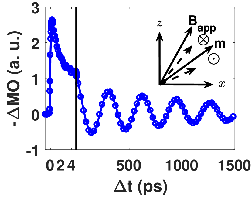
Figure 1: Representative laser-induced magnetization dynamics for a 10 nm permalloy (Ni₈₁Fe₁₉) film with an external field $B_{app}$ = 0.15 T applied almost perpendicular to the film plane DallaLonga08 . The black vertical line highlights $\Delta t$ = 5 ps, where the change of time scale occurs. Dashed arrows in the inset give schematically the effective fields for initial magnetization precession after laser excitation: The dashed arrow together with the direction of its precessional torque, shown above the magnetization, corresponds to the case for permalloy, i.e. only demagnetization anisotropy is present, while the dashed arrow and torque direction below m corresponds to the presence of both demagnetization and interface anisotropy, which is appropriate for Pt/Co/Pt films. Plot of the inset is schematic and not to scale.

For a thin film of metallic ferromagnetic material under the influence of an out-of-plane field, if there is no other forms of anisotropy present except for the shape, or demagnetization, anisotropy, the effective demagnetization field decreases in magnitude for the first a few 0.1 ps, following the ultrafast demagnetization process caused by laser heating. As a result, the total effective field is further tilted out of plane, and the magnetization vector will precess instantaneously around the new effective field. Hence, in this case, the initial precession of the magnetization is towards the direction of the external field (cf. the inset to Fig. 1). This typical behaviour is routinely observed in magnetic films with easy-plane anisotropy, and an example is shown in Fig. 1 DallaLonga08 . Atomistic simulation based on the Landau-Lifshitz-Bloch equation Kazantseva08 also supported this picture Atxitia07 .

However, for thick Pt/Co/Pt films, our measurements give a completely different behaviour: the magnetization initially moves away from the direction of the external field, as plotted in Fig. 2, although static hysteresis loops determine unambiguously that the film plane is an easy-plane. A similar difference in initial precessional behaviour for thick Co films with anisotropy changing from in-plane to out-of-plane was observed in Ref. bigot05, , but no quantitative conclusion was given. If we still want to stick to the picture that the magnetization precession is initiated by ultrafast demagnetization, this discrepancy has to be resolved. Using a model description of the magnetization procession, we find that the discrepancy can be removed by considering the interface anisotropy’s different temperature dependence as compared to that of the demagnetization anisotropy, and a $\pi$ shift in phase for magnetization precession follows from this difference in temperature dependency, in consistence with both Figs. 1 and 2.

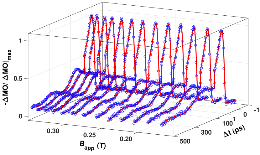
Figure 2: Magneto optical traces with various applied field ($B_{app}$) normalized to the maximal signal, $|\Delta MO|_{max}$. Note the change of scale at delay time $\Delta t$ = 1 ps. Blue circles are experimental data, and red lines are the corresponding fits. Distinctive features in magnetization dynamics induced by ultrashort laser pulses irradiating on ferromagnetic metals are discernible: ultrafast demagnetization occurring on the timescale of $<$ 1 ps and magnetization precession on the order of $\sim$ 0.1 ns.

II Experiment

The sample investigated was a Pt (4 nm)/Co (4 nm)/Pt (2 nm) film made by DC magnetron sputtering onto a Boron doped Silicon wafer with 100 nm thermally oxidized SiO₂. The base pressure of the sputtering chamber was 5.0 $\times$ 10^-8 mbar. The sputtering pressure for Pt was 3.0 $\times$ 10^-3 mbar, while it was 1.0 $\times$ 10^-2 mbar for Co. The sputtering rate is 1.16 Å/s for Pt and 0.29 Å/s for Co. Time-resolved magneto optical Kerr effect (TRMOKE) measurements were performed using a pulsed Ti:Sapphire laser with central wavelength 780 nm, pulse width 70 fs and repetition rate 80 MHz. Both pump and probe beams were focused onto the sample at almost normal incidence, hence the measured TRMOKE signal is most sensitive to the out-of-plane ($z$) component of the magnetization. The laser pump pulses induced, delay time ($\Delta t$) dependent Kerr rotation was recorded using a double modulation technique koopmans00 . In the TRMOKE measurements, the external magnetic field was applied almost normal to the film ($xy$) plane, in order to tilt the magnetization out of the film plane.

III Theoretical model

In our model description, the ultrafast demagnetization is described by the microscopic three temperature model (M3TM) koopmans10 , and the transverse relaxation of magnetization is given by the phenomenological LLG equation llg1 ; llg2 . Hence, if only heat dissipation along the film thickness is considered, the magnetization dynamics is given by three coupled differential equations koopmans10 ,

$$C_{e}\frac{dT_{e}}{dt} = \nabla_{z}(\kappa\nabla_{z}T_{e})+g_{ep}(T_{p}-T_{e})+P(t),$$

$$C_{p}\frac{dT_{p}}{dt} = g_{ep}(T_{e}-T_{p}),$$

$$\frac{d\textbf{m}}{dt} = RT_{p}\left(1-m\coth\left(\frac{mT_{C}}{T_{e}}\right)\right)\textbf{m}-\gamma\left(\textbf{m}\times\textbf{B}+\alpha\,\frac{\textbf{m}}{m}\times(\textbf{m}\times\textbf{B})\right).$$ (1)

$T_{e}$ and $T_{p}$ are the electron and phonon temperatures, $C_{e}=\gamma T_{e}$ and $C_{p}$ are the corresponding heat capacities. For a free electron gas, $\gamma=\pi^{2}D_{F}k_{B}^{2}/3V_{at}$ with $D_{F}$ the electronic density of states at the Fermi energy, $k_{B}$ the Boltzmann constant and $V_{at}$ the atomic volume. $\nabla_{z}$ denotes the $z$ component of the gradient operator. Source term $P(t)$ is related to the heating effect caused by laser pulses, which are assumed to couple directly to the electron subsystem. The three subsystems are assumed to be at equilibrium, energy and angular momentum only flow between them. m = M/$M_{0}$, whose magnitude is $m$, is the magnetization vector normalized to the zero temperature saturation magnetization $M_{0}$, $\gamma$ is the gyromagnetic ratio, and $\alpha$ is the phenomenological Gilbert damping constant. B is the total effective magnetic field, including the external, anisotropy and demagnetizaion field contributions. $T_{C}$ is the Curie temperature, $\kappa$ is the electronic thermal conductivity constant of the ferromagnetic metal, and $g_{ep}$ is the phenomenological electron-phonon coupling constant. $g_{ep}$ is assumed to be a constant, although it is actually a temperature dependent quantity Lin08 . Microscopically, $g_{ep}$ is given by

$$g_{ep}=\frac{3\pi}{2}\frac{D_{F}^{2}D_{p}E_{D}k_{B}}{V_{at}\hbar}\lambda_{ep}^{2},$$ (2)

where $\hbar$ is the reduced Planck’s constant, $D_{p}$ the number of atoms per atomic volume, $E_{D}$ the Debye energy, and $\lambda_{ep}$ the microscopic electron-phonon coupling constant. Constant $R$ determines the demagnetization rate, and is related to the spin-flip probability $\alpha_{sf}$ during electron-phonon collisions, mediated by the spin-orbit coupling, through

$$R=\frac{8\alpha_{sf}g_{ep}k_{B}T_{C}}{E_{D}^{2}\mu_{at}}$$ (3)

with $\mu_{at}$ the number density of Bohr magnetons for the ferromagnet. Compared to the M3TM koopmans10 , the main modification made here is the addition of the transverse relaxation term to the equation of motion for the magnetization vector. In spirit, the separation of the magnetization dynamics into longitudinal and transverse relaxations used here is similarly employed in the LLB equation Kazantseva08 and the self-consistent Bloch equation Xu12 . The only difference lies in the longitudinal relaxation term, which is given here by the M3TM koopmans10 .

It is well known that, at Pt/Co interfaces, the interface anisotropy is perpendicular to the film plane, due to the 3d-5d hybridization there Bruno89 ; Stohr99 . Assuming negligible bulk anisotropy, the total anisotropy is a sum of the interface anisotropy and the demagnetization anisotropy,

$$E_{A}=-\left(K_{s}\frac{m^{3}(T_{p})}{m^{2}}(\delta(z)+\delta(z-z_{0}))-K_{d}\right)m_{z}^{2},$$ (4)

where $K_{s}$ and $K_{d}=\mu_{0}M_{0}^{2}/2$ are the temperature independent, interface and demagnetization anisotropy constants. $z=0$ and $z=z_{0}$ correspond to the two Co/Pt interfaces. The temperature dependence of the interface anisotropy is taken into account explicitly in Eq. (4) by the term cubic Callen65 ; kisielewski12 in $m$. Note we have postulated that the interface anisotropy is sensitive to the lattice temperature $T_{p}$, as it is primarily determined by the crystal field bigot05 . Due to the interface character of $K_{s}$, there is a critical Co thickness where transition from out-of-plane to in-plane magnetized configuration occurs. This thickness is around 1 nm for our sputtered samples Lavrijsen11 . Hence for the 4 nm Co film considered here, the demagnetization anisotropy dominates over the interface anisotropy, and the film plane is the magnetic easy plane. Corresponding to Eq. (4), the anisotropy field is given by

$$\textbf{B}_{K}=\left(B_{s}\frac{m^{3}(T_{p})}{m^{2}}-B_{d}\right)m_{z}\hat{\textbf{e}}_{z}=(B_{A}+B_{D})\hat{\textbf{e}}_{z},$$ (5)

where $B_{s}=2K_{s}/M_{0}$, $B_{d}=\mu_{0}M_{0}$ and $\hat{\textbf{e}}_{z}$ is a unit vector perpendicular to the film plane. The Dirac delta functions are omitted.

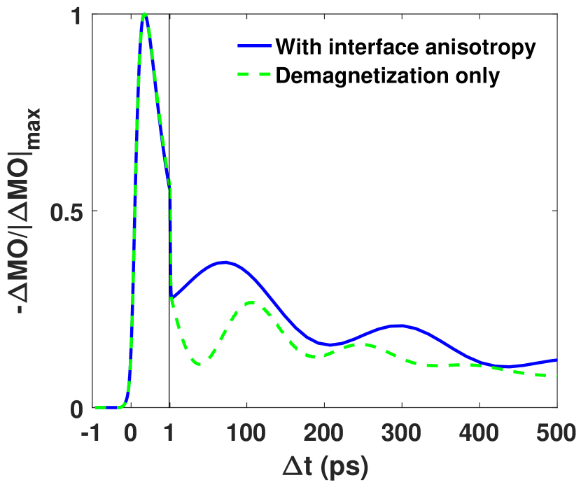
Figure 3: Simulated magnetization dynamics with $B_{app}$ = 0.35 T in the presence of the interface anisotropy or not. The transition of time scale at $\Delta t$ = 1 ps is marked by the vertical black line.

In order to numerically study the laser induced magnetization dynamics, the Co film was divided into four layers. The top layer and the bottom layer are affected by both the interface anisotropy field and the demagnetization field, while the middle layers are only influenced by the demagnetization field, which is obtainable from Eq. (5) by setting $B_{s}=0$. The exchange coupling between adjacent layers $i$ and $j$ is modelled by the usual expression

$$E_{X}=\frac{A}{d^{2}}\textbf{m}_{i}\cdot\textbf{m}_{j},$$ (6)

with $d$ = 1 nm being the separation between adjacent layers and $A$ = 28 pJ/m the exchange stiffness constant for thin film Co Liu96 ; Grimsditch97 . The laser pulse $P(t)$ was modeled by a gaussian function with group velocity dispersion Diels06 . The optical penetration depth at 780 nm of Co is 13.5 nm Krinchik68 . Except for the magnitude of the laser pulse, all other optical parameters used in the simulation were extracted from numerically fitting the short timescale ($<$1 ps) demagnetization data, using a phenomenological model given in Ref. Malinowski08, . Bulk magnetic parameters Stohr06 , $T_{C}$ = 1388 K, $V_{at}$ = 11.1 ų, $M_{0}$ = 1.72 $\mu_{B}$/$V_{at}$, $\mu_{at}$ = 1.72/$V_{at}$, were adapted in the fit to experimental data using Eq. (1). The Debye energy $E_{D}$ = 38.4 meV of Co kittel05 was also fixed in the fit to data. The thermal conductivity of a 15 nm thick Co film $\kappa$ = 40 W/m K Dejene12 was used to simulate the heat flow between individual magnetic layers. The heat exchange between the Co film and the substrate is treated simply by a phenomenological thermal conductivity $\kappa_{sub}$, which is varied to fit the data. The substrate temperature is set to the ambient temperature, $T_{am}$ = 300 K.

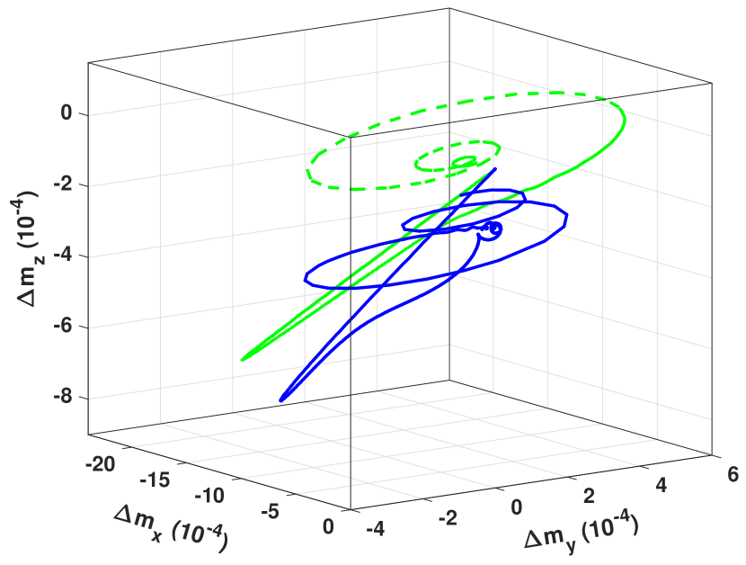
Figure 4: Simulated magnetization trajectories with $B_{app}$ = 0.29 T in the presence of the interface anisotropy (solid blue curve) or not (dashed green curve). For clarity, the trajectory with only demagnetization is scaled up by a factor of two along the $z$ direction.

IV Results

Experimental TRMOKE traces and best fits are shown in Fig. 2, after subtracting the state filling effect contribution koopmans00prl at $\Delta t$ = 0 to the experimental data. In fitting to the experimental data, the measured magneto-optical signal, $MO$, is assumed to have contributions from all three components of the magnetization vector Yang93 ; Qiu00 , $MO\propto m_{z}+\alpha_{x}m_{x}+\alpha_{y}m_{y}$, given that in our experimental setup, the probe light is not exactly normal to the film plane. Then the variation of the magneto optical signal, $\Delta MO$, which is defined as the difference after and before the arrival of the laser pulse, is normalized to the maximal demagnetization, $|\Delta MO|_{max}$, as shown in Fig. 2. The normalized data is then fitted by Eq. (1). Details of the fitting procedure can be found in Ref. koopmans10, . It can be seen from Fig. 2 that the overall agreement between experiment and theory is satisfactory, considering the crudeness of our model. This shows that the main physics is capture by the simple Eq. (1). The relevant physical parameters obtained from the best fits are $\alpha_{sf}$ = 0.16 $\pm$ 0.01, $\alpha$ = 0.07 $\pm$ 0.02, $\gamma$ = 0.164 $\pm$ 0.006 THz/T, $K_{s}$ = 1.50 $\pm$ 0.01 mJ/m², $\lambda_{ep}$ = 11.3 $\pm$ 0.3 meV. The errors given are the standard deviation of fitted values corresponding to different applied field $B_{app}$. The fitted $\gamma$ corresponds to a Landé g-factor $g$ = 1.86 $\pm$ 0.07, which is very close to the free electron value. The interface anisotropy gives an out-of-plane to in-plane transition thickness around 2.3 nm at zero temperature. This value is two times of the experimental value of about 1 nm. Since we used the bulk $T_{C}$ and $\mu_{at}$ in the fitting procedure, this difference is still acceptable. Finally, the Elliott-Yafet spin-flip probability $\alpha_{sf}$ and the electron-phonon coupling constant $\lambda_{ep}$ are comparable to those obtained in Ref. koopmans10, .

Further insights can be provided by the fitting procedure. To confirm that our model can actually reproduce the characteristic difference of the initial magnetization precession, we can set the interface anisotropy constant to zero and keep other parameters intact, thus eliminating the effect of the interface anisotropy and retaining only the demagnetization effect. The result for $B_{app}$ = 0.29 T is shown in Fig. 3. The theoretical curves of Fig. 3 demonstrate clearly the effect of the interface anisotropy and the different behaviours for the initial magnetization precession are in qualitative agreement with what we can expect. To see more clearly the magnetization dynamics and the difference in the initial precession, we plot in Fig. 4 the trajectories calculated for the top Co layer using the same set of parameters with or without the interface anisotropy. It can be easily seen that, in the presence of only the demagnetization field, the magnetization vector keeps moving upward after the ultrafast demagnetization and recovery process, continuing the trend of the magnetization recovery; while if the additional interface anisotropy is present, the magnetization’s initial precession is downward and against the tendency of the magnetization recovery. The net effect of the competition between the two forms of anisotropy is an almost $\pi$ change in the initial phase of magnetization precession.

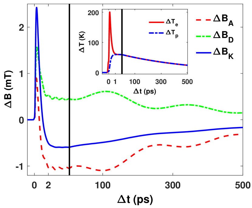
Figure 5: Dynamic evolution of the interface anisotropy field ($B_{A}$, dashed line), the demagnetization field ($B_{D}$, dash-dotted line) and the total effective field ($B_{K}$, solid line) for the top Co layer with $B_{app}$ = 0.29 T. The inset shows correspondingly the change of the electron temperature and the lattice temperature with delay time $\Delta t$. Note the change of scale at $\Delta t$ = 5 ps (2 ps in the inset) delineated by the vertical solid line. The small amplitude ringing structure visible in $\Delta B_{D}$ and $\Delta B_{A}$ is caused by the interlayer exchange coupling. It attenuates to zero in about 20 ps.

The time evolution of the total anisotropy field $B_{K}$ for the top Co layer is plotted in Fig. 5, together with its two competing components, the interface anisotropy field and the demagnetization field. The main characteristics of Fig. 5 is that, while the short timescale variation of $B_{D}$ and $B_{A}$ is both positive, $\Delta B_{D}$ and $\Delta B_{A}$ are of opposite signs at large timescale. This competition results in a negative anisotropy change, as shown in Fig. 2. The positive change of the demagnetization field is easily understandable. From Eq. (5), $\Delta B_{D}$ is essentially the change of the $z$ component of the magnetization vector. With the elevation of temperature (c.f. inset of Fig. 5), the magnitude of the magnetization vector is always reduced, therefore the change of the demagnetization field is always positive. The sign change of $\Delta B_{A}$ is intriguing. It is a natural result of the dynamic evolution of $T_{e}$ and $T_{p}$, which is itself the driving force for the ultrafast demagnetization observed at short timescale ($\Delta t<$ 1 ps in Fig. 2). As can be seen in the inset of Fig. 5, before the equilibrium is reached, the electron temperature $T_{e}$ is higher than the phonon temperature $T_{p}$. From Eq. (5), a higher $T_{e}$, whose direct consequence is a smaller $m$ ($<m(T_{p})$), will give a positive change of $B_{A}$, compared with the value before the arrival of the laser pulses. Once an equilibrium is established between $T_{e}$ and $T_{p}$ (Actually, in the inset of Fig. 5, there is a small amplitude overshooting of the phonon temperature, which is solely resulted from the fact that only the heat dissipation due to electron heat conduction is considered in Eq. (1)), their common value is still higher than the ambient temperature, $T\approx T_{e}\approx T_{p}>T_{am}$. This results in $B_{A}\propto mm_{z}(T)$, which is smaller than its corresponding value at ambient temperature, assuming the polar angle of m (hence $m_{z}$) is not increased in the whole process (Fig. 5, $\Delta B_{D}$ curve). The resulted change of anisotropy is thus negative. The above analysis qualitatively explains the change of sign for $\Delta B_{K}$, and hence the initial phase of the magnetization precession. Without the sign change in $\Delta B_{K}$, the magnetization precession will follow the $\Delta B_{D}$ curve. Therefore, the agreement between our experiment and theory affords a holistic picture for laser-induced magnetization precession in ferromagnetic metal films: the driving force behind the magnetization precession is the dynamic evolution of the anisotropy field, which is directly derived from the equilibration process of the electron and phonon subsystems initiated by irradiation of ultrashort laser pulses.

Figure 6: Phase fitted from the measured data, simulated $m_{z}$ with the inclusion of the interface anisotropy, labeled as both, and with the demagnetization field only. The lines are Linear fittings to the theoretical data. For clarity, $\omega$ for the data with only demagnetization field is scaled down by a factor of 1.53.

According to the distinct characteristics of the magnetization dynamics on both the short and long time scales, we can separate the magnetization dynamics into two stages: the ultrafast demagnetization, including the following recovery, stage and the magnetization precession stage. If we are only interested in the magnetization precession occurring on the 0.1 ns time scale, the effect of the ultrashort laser pulses, mediated through the elevated temperature for electrons and phonons, can be viewed as an impulse to the magnetization, similar in nature to the impulse given to a football to kick it off. Then the net effect of the laser irradiation is just to initiate the observed magnetization precession, which is characterized by an initial phase $\phi_{0}$ at delay time $\Delta t_{0}$ in the form of $\sin(\omega(\Delta t-\Delta t_{0})+\phi_{0})$. The initial, or incubation, delay time $\Delta t_{0}$ is a measure of how rapid a magnetization precession is established after the irradiation of laser pulses, with $\phi_{0}$ being the corresponding phase. Experimentally, only the combination $\phi=\phi_{0}-\omega\Delta t_{0}$ can be determined by fitting the measured long-term oscillation to an attenuated sine function Schellekens13 ,

$$-\Delta MO=A_{1}+A_{2}e^{-\Delta t/\tau_{e}}+\frac{A_{3}}{\sqrt{1+\Delta t/\tau_{0}}}+A_{4}e^{-\Delta t/\tau_{d}}\sin(\omega\Delta t+\phi).$$ (7)

The fitted phase $\phi$ is plotted in Fig. 6. However, the fact that the our measured signal $\Delta MO$ is related to a linear combination of all three components of the time-varying magnetization, rather than the pure $z$ component, complicates further the determination of $\phi_{0}$. To determine unambiguously both $\Delta t_{0}$ and $\phi_{0}$, we have performed simulations using the fitted parameters for various external fields, and then fit the oscillation for the $z$ component of m, $m_{z}$, to the same fitting function, Eq. (7). The slope and intercept of the fitted effective initial phase $\phi=\phi_{0}-\omega\Delta t_{0}$ as a function of $\omega$ gives $\Delta t_{0}$ and $\phi_{0}$ separately. The results obtained using this procedure are $\Delta t_{0}=11\pm 2$ ps and $\phi_{0}/\pi=1.72\pm 0.04$ in the presence and $\Delta t_{0}=1.9\pm 0.4$ ps and $\phi_{0}/\pi=0.71\pm 0.02$ in the absence of the interface anisotropy. The phase shift caused by the presence of the interface anisotropy can be approximated as $\pi$ within uncertainty margin.

V Conclusion

In summary, the laser-pumped magnetization precession in Pt/Co/Pt thin film system with perpendicular interface anisotropy was investigated by time resolved magneto optical Kerr effect. Based on a microscopic three temperature model, a model description of the magnetization precession was proposed. The agreement between theory and experiment provides insight into the different roles played by the demagnetization field and the interface anisotropy field in laser-induced magnetization precession. More specifically, the initial phase of the precession is determined by a competition between the dynamic interface anisotropy field and the demagnetization field, which follow the phonon temperature and mainly electron temperature respectively. This competition results in a $\pi$ phase shift for magnetization precession in the presence of the interface anisotropy, besides the ubiquitous demagnetization anisotropy.

- (1) E. Beaurepaire, J. C. Merle, A. Daunois, and J.-Y. Bigot, Phys. Rev. Lett. 76, 4250 (1996).
- (2) A. Kirilyuk, A. V. Kimel, and Th. Rasing, Rev. Mod. Phys. 82, 2731 (2010).
- (3) G. P. Zhang and W. Hübner, Phys. Rev. Lett. 85, 3025 (2000).
- (4) B. Koopmans, J. J. M. Ruigrok, F. Dalla Longa, and W. J. M. de Jonge, Phys. Rev. Lett. 95, 267207 (2005).
- (5) B. Koopmans, G. Malinowski, F. Dalla Longa, D. Steiauf, M. Fähnle, T. Roth, M. Cinchetti, and M. Aeschlimann, Nat. Mater. 9, 259 (2010).
- (6) T. Griepe and U. Atxitia, Phys. Rev. B 107, L100407 (2023).
- (7) E. Carpene, E. Mancini, C. Dallera, M. Brenna, E. Puppin, and S. De Silvestri, Phys. Rev. B 78, 174422 (2008).
- (8) M. Krauss, T. Roth, S. Alebrand, D. Steil, M. Cinchetti, M. Aeschlimann, and H. C. Schneider, Phys. Rev. B 80, 180407 (2009).
- (9) J.-Y. Bigot, M. Vomir, and E. Beaurepaire, Nat. Phys. 5, 461 (2009).
- (10) M. Battiato, K. Carva, and P. M. Oppeneer, Phys. Rev. Lett. 105, 027203 (2010).
- (11) M. Battiato, K. Carva, and P. M. Oppeneer, Phys. Rev. B 86, 024404 (2012).
- (12) B. Y. Mueller, T. Roth, M. Cinchetti, M. Aeschlimann, and B. Rethfeld, N. J. Phys. 13, 123010 (2011).
- (13) M. van Kampen, C. Jozsa, J. T. Kohlhepp, P. LeClair, L. Lagae, W. J. M. de Jonge, and B. Koopmans, Phys. Rev. Lett. 88, 227201 (2002).
- (14) M. van Kampen, B. Koopmans, J. T. Kohlhepp, and W. J. M. de Jonge, J. Magn. Magn. Mater. 240, 291 (2002).
- (15) J.-Y. Bigot, M. Vomir, L. H. F. Andrade, and E. Beaurepaire, Chem. Phys. 318, 137 (2005).
- (16) F. Dalla Longa, Laser-induced magnetization dynamics: an ultrafast journey among spins and light pulses, p. 87, PhD thesis, Eindhoven University of Technology, The Netherlands, 2008 (https://doi.org/10.6100/IR635203).
- (17) N. Kazantseva, D. Hinzke, U. Nowak, R. W. Chantrell, U. Atxitia, and O. Chubykalo-Fesenko, Phys. Rev. B 77, 184428 (2008).
- (18) U. Atxitia, O. Chubykalo-Fesenko, N. Kazantseva, D. Hinzke, U. Nowak, and R. W. Chantrell, Appl. Phys. Lett. 91, 232507 (2007).
- (19) L. D. Landau, E. M. Lifshitz, and L. P. Pitaevski, Statistical Physics, Part 2, 3rd ed. (Pergamon, Oxford), 1980.
- (20) T. L. Gilbert, IEEE Trans. Mag. 40, 3443 (2004).
- (21) Z. Lin, L. V. Zhigilei, and V. Celli, Phys. Rev. B 77, 075133 (2008).
- (22) L. Xu and S. Zhang, Physica E 45, 72 (2012).
- (23) B. Koopmans, M. van Kampen, J. T. Kohlhepp, and W. J. M. de Jonge, J. Appl. Phys. 87, 5070 (2000).
- (24) P. Bruno, Phys. Rev. B 39, 865 (1989).
- (25) J. Stöhr, J. Magn. Magn. Mater. 200, 470 (1999).
- (26) E. Callen and H. B. Callen, Phys. Rev. 139, A455 (1965).
- (27) K. Kisielewski, A. Kirilyuk, A. Stupakiewicz, A. Maziewski, A. Kimel, Th. Rasing, L. T. Baczewski, and A. Wawro, Phys. Rev. B 85, 184429 (2012).
- (28) R. Lavrijsen, Another spin in the wall: Domain wall dynamics in perpendicularly magnetized devices, p. 43, PhD thesis, Eindhoven University of Technology, The Netherlands, 2011 (https://doi.org/10.6100/IR693486).
- (29) X. Liu, M. M. Steiner, G. A. Prinz, R. F. C. Farrow, and G. Harp, Phys. Rev. B 53, 12166 (1996).
- (30) M. Grimsditch, E. E. Fullerton, and R. L. Stamps, Phys. Rev. B 56, 2617 (1997).
- (31) J.-C. Diels and W. Rudolph, Ultrashort laser pulse phenomena, 2nd ed. (Academic Press, San Diego), 2006.
- (32) G. S. Krinchik and V. A. Artemjev, J. Appl. Phys. 39, 1276 (1968).
- (33) G. Malinowski, F. Dalla Longa, J. H. H. Rietjens, P. V. Paluskar, R. Huijink, H. J. M. Swagten, and B. Koopmans, Nat. Phys. 4, 855 (2008).
- (34) J. Stöhr and H. C. Siegmann, Magnetism: From Fundamentals to Nanoscale Dynamics, (Springer, Berlin), 2006.
- (35) C. Kittel, Introduction to solid state physics, 8th ed. (John Wiley & Sons, New Jersey), 2005.
- (36) F. K. Dejene, J. Flipse, and B. J. van Wees, Phys. Rev. B 86, 024436 (2012).
- (37) B. Koopmans, M. van Kampen, J. T. Kohlhepp, and W. J. M. de Jonge, Phys. Rev. Lett. 85, 844 (2000).
- (38) Z. J. Yang and M. R. Scheinfein. J. Appl. Phys. 74, 6810 (1993).
- (39) Z. Q. Qiu and S. D. Bader, Rev. Sci. Instrum. 71, 1243 (2000).
- (40) A. J. Schellekens, L. Deen, D. Wang, J. T. Kohlhepp, H. J. M. Swagten, and B. Koopmans, Appl. Phys. Lett. 102, 082405 (2013).